Exact WKB methods in $SU(2)$ $N_{f}=1$

Abstract

We study in detail the Schrödinger equation corresponding to the four dimensional $SU(2)$ ${\cal N}=2$ SQCD theory with one flavour. We calculate the Voros symbols, or quantum periods, in four different ways: Borel summation of the WKB series, direct computation of Wronskians of exponentially decaying solutions, the TBA equations of Gaiotto-Moore-Neitzke/Gaiotto, and instanton counting. We make computations by all of these methods, finding good agreement. We also study the exact quantization condition for the spectrum, and we compute the Fredholm determinant of the inverse of the Schrödinger operator using the TS/ST correspondence and Zamolodchikov’s TBA, again finding good agreement. In addition, we explore two aspects of the relationship between singularities of the Borel transformed WKB series and BPS states: BPS states of the 4d theory are related to singularities in the Borel transformed WKB series for the quantum periods, and BPS states of a coupled 2d+4d system are related to singularities in the Borel transformed WKB series for local solutions of the Schrödinger equation.

1 Introduction

This paper concerns a detailed exploration of the relation between Schrödinger equations and ${\mathcal{N}}=2$ supersymmetric gauge theories, from several different points of view. We focus on one particular example, the $SU(2)$ theory with one fundamental hypermultiplet. In this introduction we briefly recall the main players in this story, describe the example we study, and indicate some of the highlights.

1.1 Quantum periods

Consider a Schrödinger equation, of the form

$$\left(-\hbar^{2}\partial_{x}^{2}+V(x)-E\right)\psi(x,\hbar)=0,$$ (1.1)

with a confining potential $V(x)$. Then a well-known problem is to identify the bound state energies, i.e. the values $E(\hbar)$ for which there exists a solution $\psi(x,\hbar)$ on the real line $x\in\mathbb{R}$ such that $\psi(x,\hbar)$ decays exponentially as $x\to\infty$ and as $x\to-\infty$.

More generally, we may consider an equation (1.1) where $x$ and $\hbar$ are allowed to be complex, and $V(x)$ is a holomorphic or meromorphic function. Then the potential may not be confining on the real line, but we can pick a more general contour where it is confining, and then ask for the existence of a solution which is exponentially decaying at both ends of the contour. This problem again determines some discrete energies $E(\hbar)$, which we may think of as generalized bound states, or resonances.

One of the important insights of the exact WKB method bpv ; voros-quartic ; voros ; ddpham ; reshyper is that the (generalized) bound state energies can be usefully expressed as solutions of an exact quantization condition. The exact quantization condition is an algebraic equation in terms of quantities $\mathcal{X}_{\gamma}=\exp\Pi_{\gamma}$ labeled by cycles $\gamma$ on the spectral curve bpv

$$\Sigma=\{y^{2}=V(x)-E\}.$$ (1.2)

The $\Pi_{\gamma}$ are the quantum periods. Up to a factor of $\hbar$, they can be thought of as an $\hbar$-deformation of the classical periods $Z_{\gamma}=\oint_{\gamma}\sqrt{V(x)-E}\,\mathrm{d}x$; indeed, they are defined by Borel summation of the series $\hbar^{-1}\oint_{\gamma}Y(x,\hbar)\mathrm{d}x$, where $Y(x,\hbar)=\sqrt{V(x)-E}+\sum_{n\geq 1}\hbar^{n}Y_{n}$ is the exponent in the WKB construction of solutions to the Schrödinger equation (1.1).

There is a connection between some Schrödinger equations (1.1) and ${\mathcal{N}}=2$ supersymmetric gauge theories placed in the Nekrasov-Shatashvili (NS) limit of the $\Omega$-background. In this connection the spectral curve (1.2) is identified as the Seiberg-Witten (SW) curve of the field theory, $\sqrt{V(x)-E}\,\mathrm{d}x$ is the Seiberg-Witten differential, and $\hbar$ is identified with the $\Omega$-background parameter $\epsilon_{1}$. In particular, the classical periods $Z_{\gamma}$ control the central charges and masses of BPS states, while the quantum periods $\Pi_{\gamma}$ can be computed in terms of the Nekrasov-Shatashvili instanton partition function. This connection has been derived from various different points of view, including direct gauge theory computations and class $S$ constructions using the AGT correspondence; see e.g. ns ; nrs ; Nekrasov:2010ka ; Drukker:2009id ; Alday:2009fs ; Maruyoshi:2010iu ; Jeong:2018qpc ; mirmor . Some recent papers which discuss quantum periods and their relation to four dimensional ${\mathcal{N}}=2$ theories are kpt ; Emery:2019znd ; Dumas:2020zoz ; Ito:2018eon ; Ito:2019twh ; Hollands:2019wbr ; Fioravanti:2019awr ; Yan:2020kkb ; gm3 ; Hatsuda_2018 ; Imaizumi:2021cxf ; Emery:2020qqu ; Aminov:2020yma ; Ito:2021boh .

1.2 The $SU(2)$ $N_{f}=1$ equation

In this paper we consider a specific example of (1.1):

$$\left(-\hbar^{2}\partial_{x}^{2}+\left(\frac{1}{2}\Lambda^{2}\operatorname{{\rm e}}^{-x}+2m\Lambda\operatorname{{\rm e}}^{x}-\Lambda^{2}\operatorname{{\rm e}}^{2x}\right)-E\right)\psi(x)=0.$$ (1.3)

This equation corresponds to ${\mathcal{N}}=2$ supersymmetric Yang-Mills theory with gauge group $SU(2)$ and $N_{f}=1$; $\Lambda\in\mathbb{C}^{\times}$ is the dynamical scale, $m\in\mathbb{C}$ is the hypermultiplet mass, and $E\in\mathbb{C}$ parameterizes the Coulomb branch.

1.3 Computing the quantum periods

Much of the utility of the quantum periods comes from the fact that they can be understood and computed from many different points of view. In Sections 3-6 below we compute the quantum periods of the equation (1.3), at various points of the parameter space, in four different ways:

1. Padé-Borel summation (Section 3): As we have explained above, the $\Pi_{\gamma}$ are defined by Borel summation of integrals $\hbar^{-1}\oint_{\gamma}Y(x,\hbar)\,\mathrm{d}x$. We compute this series numerically to high order in $\hbar$, and then use the method of Padé-Borel summation to produce numerical approximations $\Pi^{\mathrm{PB}}_{\gamma}$ of $\Pi_{\gamma}$.

2. Wronskians (Section 4): The equation (1.3) admits three distinguished solutions $\psi_{1}$, $\psi_{2}$, $\psi_{3}$ which have exponential decay along three distinguished directions in the $x$-plane; e.g. when $\hbar,\Lambda>0$ these directions are $x\to-\infty$, $x\to\infty-\frac{1}{2}{\mathrm{i}}\pi$, $x\to\infty+\frac{1}{2}{\mathrm{i}}\pi$ respectively. The $\mathcal{X}_{\gamma}$ can be expressed directly in terms of combinations of Wronskians of the solutions $\psi_{i}$ and their images under the monodromy operation of continuation $x\to x+2\pi{\mathrm{i}}$; see e.g. (4.10)-(4.12) below for examples of such formulas. By direct numerical integration of (1.3) we can thus compute numerical approximations $\mathcal{X}^{\mathrm{SS}}_{\gamma}$ of $\mathcal{X}_{\gamma}$.

3. TBA equations (Section 5.1): The $\mathcal{X}_{\gamma}$ are (conjecturally) solutions of certain integral equations given in gmn ; Gaiotto:2014bza , closely related to the ODE/IM correspondence ddt . These equations are formulated in terms of the classical periods (central charges) and the BPS state spectrum of the theory. We solve these integral equations numerically, for parameters lying in the strong coupling region (in this region the BPS spectrum is finite, which makes the equations much simpler to deal with), and thus obtain numerical approximations $\Pi^{\mathrm{TBA}}_{\gamma}$ of $\Pi_{\gamma}$.

4. Instanton counting (Section 6): As we have recalled above, the $\Pi_{\gamma}$ can be computed from the Nekrasov-Shatashvili instanton partition function in the $SU(2)$ $N_{f}=1$ theory. We carry out this computation numerically, summing the instanton series to sufficiently high order in $\Lambda$, to obtain approximations $\Pi^{\mathrm{inst}}_{\gamma}$ of $\Pi_{\gamma}$.

Various relations between these methods have been proven or conjectured in the literature. Although the details are complex one can roughly summarize as follows:

• The equivalence between methods 1 and 2 is a theorem, following from results in the exact WKB literature, as explained most precisely in in-exactwkb ; see also Hollands:2019wbr for a different route to deriving this equivalence, closer to our point of view in this paper. The recent nikolaev2020exact gives a sharp treatment of the necessary facts from exact WKB.

• The equivalence between methods 2 and 3 is proposed in Gaiotto:2009hg ; Gaiotto:2014bza and closely related to the ODE-IM correspondence ddt ; it is not yet a mathematical theorem as far as we know.

• The equivalence between methods 2 and 4 would follow from a combination of the proposal of nrs (proven in some cases in Jeong:2018qpc ) and the results in Hollands:2013qza ; Hollands:2019wbr .

Combining these theorems and conjectures one arrives at the conclusion that all four methods should give the same results, but it is not yet a theorem in full generality. Moreover, the translation between the various methods is somewhat intricate, particularly as their equivalence is formulated in different chambers of the moduli space.. Thus in this work we set ourselves the task of working out the translation carefully in the case of the $SU(2)$ $N_{f}=1$ theory, computing at various points in the parameter space with all four methods, and comparing the results. We find good agreement: within the precision we are able to obtain, the results match. See Table 1 for some sample numerical results.

Various numerical comparisons of this sort have been made before in the literature; for example see Grassi:2019coc for comparisons between methods 1, 3, 4 in the pure $SU(2)$ theory, and ddt ; Dorey:1998pt ; Dumas:2020zoz for methods 2, 3 in Argyres-Douglas theories (note method 4 is not available in Argyres-Douglas theories at the moment, since it relies on the Lagrangian description of the theory). See also Yan:2020kkb for computations in the pure $SU(3)$ theory using method 2 and comparisons to the WKB series.

In making these comparisons, we need to be careful about the analytic structure of the quantum periods. As we review in Section 2, there is a wall-and-chamber structure in the parameter space; the quantum periods are analytic in each chamber but jump when one crosses a wall. Thus, in comparing a result computed in one chamber with the analytic continuation of a result computed in a different chamber, one has to take account of extra contributions from the walls separating the chambers. These extra contributions take the form of Kontsevich-Soibelman/cluster transformations associated to BPS states of the bulk ${\mathcal{N}}=2$ theory; their concrete form is in (2.1)-(2.3) below. We use them explicitly in Section 7 when comparing instanton counting expressions with other methods.

1.4 Fredholm determinant

Another approach to studying the Schrödinger equation (1.3) runs through the Fredholm determinant

$$D(E,\hbar)=\det\left(1-\frac{E}{{\mathrm{O}}}\right)$$ (1.4)

where ${\mathrm{O}}$ is the Schrödinger operator, with trace class inverse, acting on $L^{2}$ functions along the contour where we have a confining potential. This determinant has zeros exactly at the (generalized) bound state energies, so computing it in particular determines these energies. Moreover, it was argued in Grassi:2019coc that in some examples $D(E,\hbar)$ can be computed explicitly by using a particular limit of the TS/ST correspondence cgm ; ghm , which allows to express Fredholm determinants using topological string data. This construction has been tested in several works (see for instance mmrev and reference therein). A proof in one particular example and in a special limit was given in bgt using Painlevé equations. Recently more general corollaries of this construction have been proven in Doran:2021hcy . Nevertheless a mathematical proof in full generality is still missing.

In Section 8 we apply this approach in the example of (1.3). In particular, we give a formula (8.12) for the Fredholm determinant in terms of the instanton-counting quantities introduced in Section 6.

We also consider a TBA integral equation for $D(E,\hbar)$, introduced by Zamolodchikov in post-zamo . In general this TBA equation seems to be unrelated to the system of TBA equations obeyed by the quantum periods. However, there is one special situation where there is a relation. Namely, suppose we set $E=0$ and $m=0$. In that case the TBA equations obeyed by the quantum periods simplify, reducing to a single equation, which matches with the Zamolodchikov TBA. We describe this in Section 8.2. A very similar phenomenon was noticed in the pure $SU(2)$ theory in Grassi:2019coc . We do not have a conceptual explanation for it, in either case; it would be very interesting to find one.

1.5 Quantization condition

The equation (1.3) does not have a confining potential on the real line if we take $\Lambda$ and $\hbar$ to be real. However, if we take $\hbar$ real, $\arg\Lambda=-\frac{\pi}{6}$, and look along the line $\operatorname{Im}x=-\frac{\pi}{3}$, then we do have a confining potential (which may be real or complex, depending on the phase of $m$), so we can formulate the bound state problem. It turns out that for $m\in{\mathrm{i}}\mathbb{R}_{>0}$, the case of a real convex confining potential, this condition can be formulated very simply: it is

$$\mathcal{X}_{\gamma_{[1,0,0]}}=-1$$ (1.5)

where $\gamma_{[1,0,0]}$ is the cycle connecting the two classical turning points, shown in Figure 11 below.

In this paper we give two different routes to deriving this exact quantization condition. One, in Section 4, goes through the connection between quantum periods and Wronskians of solutions. The other, in Section 8, uses the connection between quantum periods and Fredholm determinants, combined with the relation between Fredholm determinants and instanton counting. Happily, both methods independently give the quantization condition (1.5); this provides a nice cross-check of our computations.

1.6 Comments

We comment on a few interesting points and future directions here:

• The result of instanton counting agrees directly with the quantum period only at a particular locus of the parameter space, which we call the instanton locus. This locus lies on one of the walls in the wall-and-chamber decomposition of the parameter space. The results of nrs ; Hollands:2013qza , translated to our language, amount to a determination of the instanton locus in the $SU(2)$ $N_{f}=4$ theory, and similarly Grassi:2019coc determines the chamber in the pure $SU(2)$ theory. For the $SU(3)$ $N_{f}=6$ theory the instanton locus was found in Hollands:2017ahy . In all of these examples, the instanton locus lies at weak coupling, with $\hbar$ chosen so that $\arg\hbar$ is the phase of the central charge of the vectormultiplet. In this paper we identify the instanton locus in the $SU(2)$ $N_{f}=1$ theory. We find that this locus is determined by requiring that the parameters $(\Lambda,m)$ define a positive, convex and confining potential along some line in the $x$-plane. As for the $\hbar$ parameter, we find that it again follows the same pattern as above.

  For generic complex values of the parameters, instanton counting will agree with Borel summation only after we implement an appropriate Kontsevich-Soibelman (KS) transformation. This is described in Section 7.

• We work out explicitly the transformation relating the quantum periods at weak coupling to the analytic continuation of the quantum periods from strong coupling; see (7.18)-(7.20). This transformation can be viewed as a relation between specific sorts of Fock-Goncharov-type and Fenchel-Nielsen-type coordinates, generalizing a similar (simpler) one which appears in the pure $SU(2)$ theory and was used recently in Grassi:2019coc ; Coman:2020qgf .

• As we remarked above, the singularities of the Borel transform of $\Pi_{\gamma}$ are expected to appear at the central charges of BPS particles in the ${\mathcal{N}}=2$ field theory. This phenomenon was explored numerically in Grassi:2019coc for the pure $SU(2)$ theory, and we do the same in the $SU(2)$ $N_{f}=1$ theory here. We also discuss a related statement for the singularities of the Borel transform of the WKB solutions of the Schrödinger equation (1.3): namely, these appear at the central charges of BPS solitons in a certain 2d-4d coupled system. (In practical terms this means considering integrals of the Seiberg-Witten differential along open paths instead of closed ones.) This is discussed in Section 3.4 and Appendix C.2.

• The coupled 2d-4d system should also lead to other methods of computing local solutions of the Schrödinger equation directly, by appropriate 2d-4d extensions of the methods we use here to compute quantum periods. Indeed, an extension of the TBA integral equations which should compute the solutions has been described in Gaiotto:2014bza ; it arises as the conformal limit of the 2d-4d equations of Gaiotto:2011tf . One should also be able to compute the solutions by a version of the Nekrasov-Shatashvili instanton counting in the presence of the surface defect, see for instance Maruyoshi:2010iu or Jeong:2018qpc for more recent work. It would be interesting to work this out carefully in some examples.

• In this paper we study the four-dimensional field-theoretic framework which, on the operator theory side, corresponds to studying a differential equation. It would be interesting to generalise this approach to the five-dimensional field theory setup and the corresponding difference equations, considered e.g. in acdkv . One would expect this to make contact with exponential networks eager ; Longhi:2021qvz ; longhi ; Banerjee:2020moh and BPS states of local CY threefolds dfr , see also Closset:2019juk ; Bonelli:2020dcp . It would also be interesting to understand the structure of the exact solution for the spectral theory of such difference equations proposed in ghm ; cgm ; wzh ; mz-wv .

Acknowledgements

We thank Daniele Gregori, Jie Gu, Lotte Hollands, Ahsan Khan, Marcos Mariño, and Fei Yan for helpful discussions. The work of AN is supported by National Science Foundation grant 2005312 (DMS). The work of AG is partially supported by the Fonds National Suisse, Grant No. 185723 and by the NCCR “The Mathematics of Physics” (SwissMAP).

Strong coupling region
$m=-1/10$, $\Lambda=1$, $u=0$, $\hbar=1+{\rm i}/10$
$\gamma$	$[-1,-1,1]$	$[1,0,0]$	$[0,1,1]$
$\Pi_{\gamma}^{\rm PB}$	$2.31044583$	$1.7968493$	$-2.86310004138$
	$+3.06848675{\rm i}$	$-3.5249441{\rm i}$	$+0.33203784{\rm i}$
$\Pi^{\rm TBA}_{\gamma}$	$2.3105$	$1.797$	$-2.863$
	$+3.068{\rm i}$	$-3.5249{\rm i}$	$+0.3320{\rm i}$
$\Pi^{\rm SS}_{\gamma}$	$2.31044583$	$1.7968493$	$-2.8631000414$
	$+3.06848675{\rm i}$	$-3.5249441{\rm i}$	$+0.33203784{\rm i}$
$m=-1/10$, $\Lambda=1$, $u=0$, $\hbar=\frac{8}{5}(1+{\rm i}/10)$
$\gamma$	$[-1,-1,1]$	$[1,0,0]$	$[0,1,1]$
$\Pi_{\gamma}^{\rm PB}$	$1.251837$	$1.10078$	$-1.5749919$
	$+2.10014{\rm i}$	$-2.4030{\rm i}$	$+0.225114{\rm i}$
$\Pi_{\gamma}^{\rm inst}$	$1.2518373$	$1.1007766$	$-1.5749919$
	$2.1001386{\rm i}$	$-2.4030151{\rm i}$	$+0.22511425{\rm i}$
$\Pi^{\rm TBA}_{\gamma}$	$1.252$	$1.1008$	$-1.575$
	$+2.100{\rm i}$	$-2.403{\rm i}$	$+0.2251{\rm i}$
$\Pi^{\rm SS}_{\gamma}$	$1.251837$	$1.10078$	$-1.5749919$
	$+2.10014{\rm i}$	$-2.4030{\rm i}$	$+0.225114{\rm i}$
$m=-1/10$, $\Lambda=1/5$, $u=0$, $\hbar=1+{\rm i}/10$
$\gamma$	$[-1,-1,1]$	$[1,0,0]$	$[0,1,1]$
$\Pi^{\rm inst}_{\gamma}$	$-0.07209621704459846369$	$0.79394041891943969067$	$0.52235090845775015459$
	$+1.05629021332321667555{\rm i}$	$-1.25702427315714059939{\rm i}$	$+0.07631454880066478568{\rm i}$
$\Pi^{\rm TBA}_{\gamma}$	$-0.072$	$0.794$	$0.522$
	$+1.056{\rm i}$	$-1.257{\rm i}$	$+0.0763{\rm i}$
$\Pi^{\rm SS}_{\gamma}$	$-0.07209622$	$0.793940419$	$0.52235091$
	$+1.0562902{\rm i}$	$-1.25702427{\rm i}$	$+0.07631455{\rm i}$
$m=0$, $\Lambda=1/5$, $u=0$, $\hbar=1+{\rm i}/10$
$\gamma$	$[-1,-1,1]$	$[1,0,0]$	$[0,1,1]$
$\Pi^{\rm inst}_{\gamma}$	$-0.40014633959247147382$	$0.25765417201941334603$	$0.14249216757305812778$
	$+1.05116204874070340420{\rm i}$	$-1.16973711207642800270{\rm i}$	$+0.11857506333572459850{\rm i}$
$\Pi^{\rm TBA}_{\gamma}$	$-0.400$	$0.258$	$0.142$
	$+1.051{\rm i}$	$-1.170{\rm i}$	$+0.119{\rm i}$
$\Pi^{\rm SS}_{\gamma}$	$-0.4001463396$	$0.25765417202$	$0.14249216757$
	$+1.051162049{\rm i}$	$-1.169737112{\rm i}$	$+0.118575063{\rm i}$
$m=0$, $\Lambda=1/5$, $u=0$, $\hbar=\frac{1}{3}(1+{\rm i}/10)$
$\gamma$	$[-1,-1,1]$	$[1,0,0]$	$[0,1,1]$
$\Pi^{\rm PB}_{\gamma}$	$0.940082$	$0.78280$	$-1.7228798$
	$+2.03841{\rm i}$	$-2.2823{\rm i}$	$+0.243848{\rm i}$
$\Pi^{\rm inst}_{\gamma}$	$0.9400824$	$0.782797$	$-1.7228798$
	$+2.03840655{\rm i}$	$-2.28225498{\rm i}$	$+0.2438484{\rm i}$
$\Pi^{\rm TBA}_{\gamma}$	$0.940$	$0.7828$	$-1.723$
	$+2.038{\rm i}$	$-2.282{\rm i}$	$+0.2438{\rm i}$
$\Pi^{\rm SS}_{\gamma}$	$0.940082$	$0.78280$	$-1.7228798$
	$+2.03841{\rm i}$	$-2.2823{\rm i}$	$+0.243848{\rm i}$
Continued on next page

Weak coupling region
$m=0$, $\Lambda=1/5$, $u=2$, $\hbar=1+{\rm i}/10$
$\gamma$	$[-1,-1,1]$	$[1,0,0]$	$[0,2,0]$
$\Pi_{\gamma}^{\rm PB}$	$3.562524034409252$	$8.8794275059299982$	$-24.8839030806784999581424$
	$-26.953094797469923{\rm i}$	$+25.708899620419279{\rm i}$	$+2.488390354101287262159325{\rm i}$
$\Pi^{\rm inst}_{\gamma}$	$3.562524034409252$	$8.8794275059299982$	$-24.8839030806784999581424$
	$-26.953094797469923{\rm i}$	$+25.708899620419279{\rm i}$	$+2.488390354101287262159325{\rm i}$
$\Pi^{\rm SS}_{\gamma}$	$3.562524034$	$8.8794275059$	$-24.8839030807$
	$-26.9530947975{\rm i}$	$+25.7088996204{\rm i}$	$+2.488390354101{\rm i}$
$m=0$, $\Lambda=1/5$, $u=2$, $\hbar=1$
$\gamma$	$[-1,-1,1]$	$[1,0,0]$	$[0,2,0]$
$\Pi_{\gamma}^{\rm PB}$	$6.283185528939026$	$6.283185528939026$	$-25.132742115756103$
	$-26.595529611194577{\rm i}$	$+26.595529611194577{\rm i}$	$627145534$
$\Pi^{\rm inst}_{\gamma}$	$6.283185528939026$	$6.283185528939026$	$-25.132742115756103$
	$-26.5955296111946{\rm i}$	$+26.595529611194577{\rm i}$	627145534057
$\Pi^{\rm SS}_{\gamma}$	$6.2831855289$	$6.2831855289$	$-25.13274211576$
	$-26.5955296112{\rm i}$	$+26.5955296112{\rm i}$
$m={\rm i}/10,~{}\Lambda=\operatorname{{\rm e}}^{-\frac{\pi{\rm i}}{6}},~{}u=2,~{}\hbar=1$
$\gamma$	$[-1,-1,1]$	$[1,0,0]$	$[0,2,0]$
$\Pi_{\gamma}^{\rm PB}$	$12.5407604031$	$6.948499{\rm i}$	$-25.08152080613$
	$-7.57682{\rm i}$
$\Pi^{\rm inst}_{\gamma}$	$12.5407604031$	$6.9484991958{\rm i}$	$-25.08152080613$
	$-7.576818{\rm i}$
$\Pi^{\rm SS}_{\gamma}$	$12.540760403$	$6.9484991958{\rm i}$	$-25.0815208061$
	$-7.576818{\rm i}$

Table 1: Summary of results of numerical computation of $\Pi_{\gamma}$ for various moduli, charges and values of $\hbar$. $\Pi_{\gamma}^{\rm PB}$, $\Pi_{\gamma}^{\rm SS}$, $\Pi^{\rm TBA}_{\gamma}$, $\Pi^{\rm inst}_{\gamma}$ are the quantum periods we obtain by Padé-Borel summation, small section, TBA and instanton counting methods respectively; all of them are approximations to the true $\Pi_{\gamma}$. For each point of parameter space which we study, we list results from all methods which we were able to apply at that point. We emphasize that $\Pi_{\gamma}$ denotes the canonical piecewise-analytic function discussed in Section 2 below; e.g. this is the quantity one would obtain directly by Borel summation without any further transformations.

2 Analytic structures

In what follows we are going to compute the quantum periods by various different methods and compare them. To make this comparison correctly one needs to take account of a certain wall-and-chamber structure in the parameter space, which we review here.

2.1 Walls and chambers

We consider a complex four-dimensional parameter space, consisting of the complex couplings $(m,\Lambda)$, the Coulomb branch modulus $u$, and a complex mass parameter $\hbar\neq 0$, which could be interpreted as an $\Omega$-background parameter.

In this space one has various real-codimension-1 walls defined as follows. A point $(m,\Lambda,u,\hbar)$ is on a wall if and only if the 4d field theory with couplings $(m,\Lambda)$, at the point $u$ of its Coulomb branch, has a BPS one-particle state for which the central charge $Z$ has $\arg(-Z)=\arg(\hbar)$, i.e. $Z/\hbar\in\mathbb{R}_{-}$. In this case we say that the wall supports the BPS state. Generically, each wall will support only BPS states which are mutually local with one another, i.e. their charges obey $\langle\gamma,\gamma^{\prime}\rangle=0$. The walls divide the parameter-space up into chambers.

To get some feeling for this structure let us consider slicing it along various directions. If we hold the parameters $(m,\Lambda,u)$ fixed and let only $\hbar$ vary, then the walls reduce to rays in the $\hbar$-plane. Each BPS state which exists in the theory at $(m,\Lambda,u)$ is supported by a ray in the $\hbar$-plane whose angle is $\arg(-Z)$. Since $Z$ is determined by the electromagnetic and flavor charge $\gamma$ of the state, we may also denote it as $Z_{\gamma}$. See Figure 1 for the walls in the $\hbar$-plane at two different points in $(m,\Lambda,u)$ space.

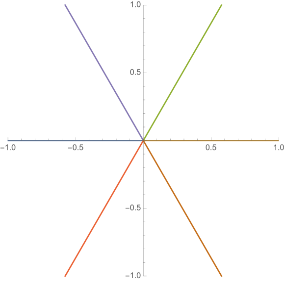
(a) The walls in the $\hbar$-plane at $m=0$, $\Lambda=1/5$, $u=0$ (strong coupling).

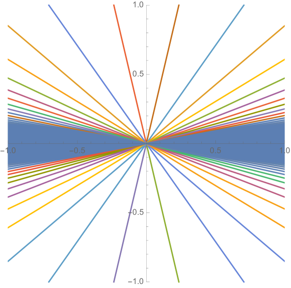
(b) The walls in the $\hbar$-plane at $m=0$, $\Lambda=1/5$, $u=2$ (weak coupling).

Figure 1: The strong coupling BPS spectrum consists of 3 hypermultiplets and their antiparticles, while the weak coupling BPS spectrum consists of 1 vectormultiplet and infinitely many hypermultiplets. There is a wall in the direction $\vartheta$ whenever there exists a BPS particle of charge $\gamma$ with $\vartheta=\arg(Z_{\gamma})$. (Generically each wall corresponds to a single particle, but in 1(b) each of the horizontal rays actually represents several BPS particles with the same phase: a vectormultiplet and two hypermultiplets. This accidental degeneracy would be broken for $m\neq 0$.) In 1(b), the rays accumulate around $\vartheta=0$, which is the phase corresponding to the vectormultiplet. This kind of accumulation happens generically in theories with higher-spin BPS particles.

As $(m,\Lambda,u)$ are varied, the quantities $Z_{\gamma}$ vary, and thus the rays move in the $\hbar$-plane. To capture this behavior it is useful to draw a different slicing, where we show one real direction in the $(m,\Lambda,u)$ parameter space, and also show the phase $\arg\hbar$. See Figure 2 for an example of this in the $SU(2)$ $N_{f}=1$ theory, and Figure 14 for an example in the simpler pure $SU(2)$ theory. Each of these figures can be thought of as a graph of the evolution of the phases of the central charges of BPS particles as we move along a curve in the Coulomb branch. Note again that when the phases collide some BPS bound states can form or decay, and thus we have different numbers of BPS states in different regions of the Coulomb branch: finitely many at strong coupling, infinitely many at weak coupling.

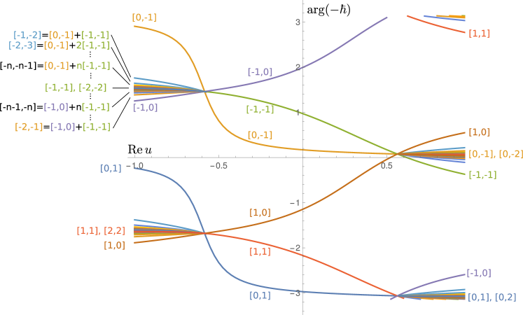
Figure 2: The BPS walls when we fix $\Lambda=1,\ m=0,\ {\rm Im}(u)=\frac{{\rm i}}{10}$. The horizontal axis is ${\rm Re}(u)$; the vertical axis is $\arg(-\hbar)\in[-\pi,\pi]$. There are 2 special points at around $u_{1}\approx-0.6+\frac{{\rm i}}{10}$ and $u_{2}\approx 0.675+\frac{{\rm i}}{10}$ where the wall of marginal stability is encountered. For ${\rm Re}(u)\in(u_{1},u_{2})$ (strong coupling) we have 3 hypermultiplets and their antiparticles, so there are 6 walls in total shown in this region. For $u<u_{1}$ or $u>u_{2}$ (weak coupling), we have infinitely many hypermultiplets. The hypermultiplet walls accumulate around the vectormultiplet wall. We list the electromagnetic charges of the particles next to their corresponding walls.

Finally we could consider holding $(m,\Lambda,\hbar)$ fixed and letting $u$ vary. In that case we get a collection of walls on the Coulomb branch. See Figure 15 for an example in the pure $SU(2)$ theory.

2.2 Chamber structure for quantum periods

The importance of this chamber structure for us is that the quantum periods $\Pi_{\gamma}(m,\Lambda,u,\hbar)$ are piecewise analytic functions on the parameter space: precisely, they are analytic in each chamber, but jump at the walls. This structure shows up in a different way in each method of computing the quantum periods:

1. In the Borel summation method, the jumps occur because of the need to move a contour of integration across a singularity in the Borel plane.

2. In the Wronskian or “small section” method, the jumps arise as follows. Each $(m,\Lambda,u,\hbar)$ determines a spectral network drawn on the $z$-plane. The spectral network can be used to give a formula for $\mathcal{X}_{\gamma}=\exp\Pi_{\gamma}$ in terms of Wronskians of solutions of the ODE (1.3). The precise expression for $\mathcal{X}_{\gamma}$ in terms of Wronskians depends on the topology of the spectral network, which in turn depends on which chamber $(m,\Lambda,u,\hbar)$ is in.

3. In the TBA method, the jumps arise again from the need to move a contour of integration across a singularity, this time a singularity in the TBA integration kernel.

4. In the instanton counting method, one does not see the jumps directly. Rather, instanton counting produces multivalued analytic functions, which can be understood as analytic continuations of the quantum periods from a specific locus in the parameter-space.

To keep track of the analytic structure, and having in mind the possibility of analytic continuation from one chamber to another, it is convenient to introduce new functions $\Pi_{\gamma}^{(m_{0},\Lambda_{0},u_{0},\hbar_{0})}(m,\Lambda,u,\hbar)$ which are defined by analytic continuation of $\Pi_{\gamma}$ from a base-point $(m_{0},\Lambda_{0},u_{0},\hbar_{0})$. Thus our convention is: when we write $\Pi_{\gamma}(m,\Lambda,u,\hbar)$ without a basepoint superscript, we mean the canonical piecewise-analytic function; when we write it with a basepoint superscript, we mean the function defined by analytic continuation from the basepoint. Since the dependence on $\hbar_{0}$ is only through $\arg\hbar_{0}$ we also sometimes use the notation $\vartheta=\arg\hbar_{0}$ and write e.g. $\Pi_{\gamma}^{\vartheta}$ instead of $\Pi_{\gamma}^{\hbar_{0}}$.

The question now naturally arises: what is the relation between the analytic continuations from different chambers? To understand this, it is sufficient to understand what happens for two chambers separated by a single wall. To be definite, let us hold $(m,\Lambda,u)$ fixed for a moment. Then the wall is just a ray in the $\hbar$-plane, at some $\arg\hbar=\vartheta_{*}$. Now we consider the relation between $\Pi_{\gamma}^{\vartheta}$ and $\Pi_{\gamma}^{\vartheta^{\prime}}$ for two different phases $\vartheta$, $\vartheta^{\prime}$ with $\vartheta<\vartheta_{*}<\vartheta^{\prime}$. In this case the relation takes the form Gaiotto:2009hg ; Gaiotto:2012rg

$$\Pi_{\mu}^{\vartheta^{\prime}}-\Pi_{\mu}^{\vartheta}=\sum_{\gamma}\langle\mu,\gamma\rangle\Omega(\gamma)\log(1-\sigma_{\mathrm{can}}(\gamma)\mathcal{X}_{\gamma}^{\vartheta}).$$ (2.1)

Here:

• The sum runs over the charges $\gamma$ of BPS states supported at the wall.

• $\Omega(\gamma)$ is the BPS index (second helicity supertrace) counting BPS states of charge $\gamma$.

• $\sigma_{\mathrm{can}}$ is a factor defined in Gaiotto:2009hg , with the property that $\sigma_{\mathrm{can}}(\gamma)=-1$ whenever $\gamma$ is the charge of a BPS hypermultiplet, and $\sigma_{\mathrm{can}}(\gamma)=1$ whenever $\gamma$ is the charge of a BPS vectormultiplet.

At first (2.1) seems to have a puzzling asymmetry: why did we write $\mathcal{X}_{\gamma}^{\vartheta}$ on the right instead of $\mathcal{X}_{\gamma}^{\vartheta^{\prime}}$? But since the BPS states supported at a generic point of the wall are all mutually local, (2.1) says that $\Pi_{\mu}^{\vartheta}=\Pi_{\mu}^{\vartheta^{\prime}}$ when $\mu$ is any charge supported at the wall. Thus we have $\mathcal{X}_{\gamma}^{\vartheta}=\mathcal{X}_{\gamma}^{\vartheta^{\prime}}$, so it did not matter which we wrote on the RHS.

The simplest and most generic case is a wall supporting a single BPS hypermultiplet of charge $\gamma$; in that case we have $\Omega(\gamma)=1$, $\sigma_{\mathrm{can}}(\gamma)=-1$, and thus the transformation becomes

$$\Pi_{\mu}^{\vartheta^{\prime}}-\Pi_{\mu}^{\vartheta}=\langle\mu,\gamma\rangle\log(1+\mathcal{X}_{\gamma}^{\vartheta}).$$ (2.2)

So far we have been discussing $\Pi_{\gamma}$ in the open chambers, but it will be important below sometimes to consider $\Pi_{\gamma}$ on the walls as well. On a wall, we define $\Pi_{\gamma}$ to be the average of the limits of its values from the two sides of the wall. Thus, the analogue of (2.1) for comparing the value on the wall to the value on one side of the wall just involves an extra factor $\frac{1}{2}$:

$$\Pi_{\mu}^{\vartheta_{*}}-\Pi_{\mu}^{\vartheta}=\frac{1}{2}\sum_{\gamma}\langle\mu,\gamma\rangle\Omega(\gamma)\log(1-\sigma_{\mathrm{can}}(\gamma)\mathcal{X}_{\gamma}^{\vartheta}).$$ (2.3)

More generally we may consider varying all the parameters $(m,\Lambda,u,\hbar)$. For example, looking at Figure 2, we see that while holding $(m,\Lambda)$ fixed, we could cross any given wall either by varying $\arg\hbar$ while holding $u$ fixed or by varying $u$ while holding $\arg\hbar$ fixed. Irrespective of which parameters we vary, the transformation associated to the wall is the same, given by (2.1).

3 Borel summation

In this section, we briefly review the exact WKB method and Padé-Borel summation, applied to the Schrödinger equation

$$\left(-\hbar^{2}\partial_{x}^{2}+P(x)\right)\psi(x)=\left(-\hbar^{2}\partial_{x}^{2}+(\frac{\Lambda^{2}\operatorname{{\rm e}}^{-x}}{2}+2m\Lambda\operatorname{{\rm e}}^{x}-\Lambda^{2}\operatorname{{\rm e}}^{2x})-E\right)\psi(x)=0,$$ (3.1)

where

$$P(x)=\left(\frac{\Lambda^{2}\operatorname{{\rm e}}^{-x}}{2}+2m\Lambda\operatorname{{\rm e}}^{x}-\Lambda^{2}\operatorname{{\rm e}}^{2x}\right)-E.$$ (3.2)

For the moment, we do not impose any reality conditions on the parameters $(m,\Lambda,E)$ or the variable $x$ in (3.1). Sometimes it is also useful to make the coordinate transformation

$$z=\operatorname{{\rm e}}^{x}\$$ (3.3)

and redefine $\psi(z)=(z)^{-\frac{1}{2}}\psi(z)$, after which (3.1) becomes

$$\left(-z^{2}\hbar^{2}\partial_{z}^{2}+(\frac{\Lambda^{2}}{2z}+2m\Lambda z-\Lambda^{2}z^{2})-(E+\frac{\hbar^{2}}{4})\right)\psi(z)=0.$$ (3.4)

Here $z$ is a coordinate on the punctured Riemann surface $C=\mathbb{CP}^{1}\backslash\{0,\infty\}$. In the rest of the manuscript we go from $x$ to $z$ interchangeably. Which variable we are using should be clear from the context.

3.1 All-orders WKB

The starting point is the all-orders WKB analysis. Let us make the following ansatz for a solution of (3.1):

$$\psi(x)=\exp\left(\frac{1}{\hbar}\int_{x_{0}}^{x}Y(x,\hbar)\mathrm{d}x\right).$$ (3.5)

Then (3.1) implies that $Y(x,\hbar)$ should satisfy the Ricatti equation

$$-\left(Y(x,\hbar)\right)^{2}-\hbar{\frac{{\rm d}}{{\rm d}x}}Y(x,\hbar)+P(x)=0\,.$$ (3.6)

We can solve (3.6) formally as a power series in $\hbar$ using the ansatz

$$Y(x,\hbar)=\sum_{n=0}^{\infty}Y^{n}(x)\hbar^{n}\,,$$ (3.7)

where $Y^{0}=\pm\sqrt{P(x)}$. We denote the two choices of sign by $Y^{0,(1)}$ and $Y^{0,(2)}$. All the higher order terms depend on which $Y^{0,(i)}$ we choose, so we denote the solutions

$$\psi^{(i)}(x)=\exp\left(\frac{1}{\hbar}\int_{x_{0}}^{x}Y^{(i)}(x,\hbar)\mathrm{d}x\right).$$ (3.8)

It is convenient to split the formal series expansion (3.7) into even and odd components as

$$Y_{\rm even}= \sum_{n=0}^{\infty}Y^{2n}(x)\hbar^{2n}\,,$$ (3.9)

$$Y_{\rm odd}= \sum_{n=0}^{\infty}Y^{2n+1}(x)\hbar^{2n+1}.$$

Then one finds that

$$Y_{\rm odd}=-{\frac{\hbar}{2}}{\frac{{\rm d}}{{\rm d}x}}\log Y_{\rm even}.$$ (3.10)

3.2 Borel summation of the local solutions

An important point is that the all-orders WKB method does not provide actual analytic solutions, but formal power series. Indeed the coefficients in (3.7) grow factorially as

$$Y^{n}\sim n!\quad\text{for}\quad n\gg 1.$$ (3.11)

Therefore, (3.7) is purely a formal expression with zero radius of convergence. Borel summation gives a way to convert this type of asymptotic series into an analytic function (for $\hbar$ lying in some half-plane). This works as follows. We consider the Borel transform of the formal series $Y(z,\hbar)$,

$$\hat{Y}(z,\zeta)=\sum_{n=0}^{\infty}\frac{Y^{n}(z)}{(n)!}\zeta^{n},$$ (3.12)

which is a convergent series for sufficiently small $\lvert\zeta\rvert$. The Borel summation $s(Y)$ is then defined by the Laplace transform

$$s(Y)(z,\hbar)=\frac{1}{|\hbar|}\int_{0}^{\infty}\hat{Y}(z,{\rm e}^{{\rm i}\arg(\hbar)}\zeta)\operatorname{{\rm e}}^{-\zeta/|\hbar|}d\zeta.$$ (3.13)

Note that in the integral (3.13), we need to analytically continue $\hat{Y}(z,\zeta)$ along the integration ray, beyond the region where the sum (3.12) converges. It is known that such an analytic continuation exists, and the integral (3.13) converges, for generic choices of $\arg(\hbar)$ MR3706198 ; nikolaev2020exact . In numerical computations, we approximate the desired analytic continuation by taking finitely many terms in the series (3.12), and then taking a Padé approximant of the resulting polynomial; this gives a rational function, meromorphic in the whole $\zeta$-plane. Substituting this rational function for $\hat{Y}(z,\zeta)$ in (3.13), we obtain an approximation to the desired $s(Y)(z,\hbar)$. This method of approximation is known as Padé-Borel summation.

For some special values of $\arg(\hbar)$, it may happen that the integral in (3.13) is not well defined, because $\hat{Y}(z,\zeta)$ has singularities along the integration contour. In this case, we say that $Y(z,\hbar)$ is not Borel summable, and consider instead the lateral Borel summation

$$s_{\pm}(Y)(z,\hbar)=\frac{1}{|\hbar|}\int_{0}^{{\rm e}^{{\rm i}0^{\pm}}\infty}\hat{Y}(z,{\rm e}^{{\rm i}\arg(\hbar)}\zeta)\operatorname{{\rm e}}^{-\zeta/|\hbar|}d\zeta.$$ (3.14)

In this paper we will never use lateral Borel summation directly; rather we always use the median summation, which is defined as

$$\overline{s}(Y)(z,\hbar)={\frac{1}{2}}\left(s_{+}(Y)(z,\hbar)+s_{-}(Y)(z,\hbar)\right).$$ (3.15)

3.3 Seiberg-Witten description of $SU(2)$ $N_{f}=1$

One powerful way of understanding the singularities in the Borel plane, and the corresponding behavior of Borel summation, is by exploiting the connection between the operators (3.1), (3.4) and Seiberg-Witten theory, which we now review.

It is well known that the classical limit of (3.4) corresponds to the Seiberg-Witten curve for four dimensional $SU(2)$ theory with $N_{f}=1$ by identifying $E=2u$; see for instance Maruyoshi:2010iu which has the same conventions we do. We recall that this Seiberg-Witten curve can be represented as

$$\Sigma=\left\{\lambda^{2}-\left(\frac{\Lambda^{2}}{2z^{3}}+\frac{2m\Lambda}{z}-\Lambda^{2}-\frac{2u}{z^{2}}\right)\mathrm{d}z^{2}=0\right\}\subset T^{*}C.$$ (3.16)

From this perspective, the label $i$ for the square-root branches in (3.8) is identified with the label of the sheets of the $2$-fold covering $\Sigma\xrightarrow{2:1}C$. For generic $u$, the quantity $P(z)$ in the parentheses has 3 zeros; we call them $z_{1}$, $z_{2}$, $z_{3}$; then $\{0,z_{1},z_{2},z_{3}\}$ are the branch points of the covering.

For any value of parameters, the electromagnetic and flavor charge lattice $\Gamma$ can be represented as a rank $3$ sublattice of $H_{1}(\overline{\Sigma},\mathbb{Z}),$ where $\overline{\Sigma}$ is obtained by filling in the punctures of $\Sigma$. We will choose a basis of $\Gamma$ for each value of parameters that we study, and thus represent the charges concretely as $\gamma_{[m,n,\mu]}$. In each case we fix a pure magnetic charge

$$\gamma_{a_{D}}\equiv\gamma_{[1,0,0]},$$ (3.17)

a pure electric charge

$$\gamma_{a}\equiv\gamma_{[0,2,0]}=2\gamma_{[0,1,0]},$$ (3.18)

and a pure flavor charge

$$\gamma_{f}\equiv\gamma_{[0,0,1]}.$$ (3.19)

In each case we take $\gamma_{f}$ to be the homology class of a loop surrounding only the irregular singularity $z=\infty$ and no other turning points or singularities.

Some examples of charges in the bases we use are shown in Figure 3 and 4(a). Note that when the parameters $(u,m,\Lambda)$ change, the positions of branch points also change; thus we have to analytically continue the branch points and the corresponding cycles. The specific choice of basis shown in 4(a) is well adapted for comparison with the instanton counting method: the vectormultiplet has charge $\gamma_{a}$, while the derivative of the prepotential corresponds to the charge $\gamma_{a_{D}}$. We discuss this in more detail in Section 6.

We also recall some standard quantities associated to the charge lattice. The antisymmetric non-degenerate intersection pairing of electromagnetic charges is given by

$$\langle\gamma,\gamma^{\prime}\rangle=\langle[n_{1},n_{2},*],[n_{1}^{\prime},n_{2}^{\prime},*^{\prime}]\rangle=n_{1}n_{2}^{\prime}-n_{2}n_{1}^{\prime}\,.$$ (3.20)

The central charge corresponding to $\gamma_{[m,n,\mu]}$ is

$$Z_{\gamma_{[m,n,\mu]}}=\oint_{\gamma_{[m,n,\mu]}}\lambda=mZ_{\gamma_{[1,0,0]}}+nZ_{\gamma_{[0,1,0]}}+\mu Z_{\gamma_{[0,0,1]}}$$ (3.21)

where $\lambda$ is the Seiberg-Witten differential.

3.3.1 A strong coupling point

As an example we can take the parameters to be $m=-1/10$, $\Lambda=1$, $u=0$. In this case we are in the strong coupling region and there are only 3 BPS hypermultiplets, with charges $\gamma_{\pm[1,0,0]}$, $\gamma_{\pm[0,1,1]}$ and $\gamma_{\pm[-1,-1,1]}$. These charges are shown in Figure 3. The corresponding central charges are

• $Z_{\gamma_{[-1,-1,1]}}=2.1922857627+3.0893009403{\rm i},$

• $Z_{\gamma_{[1,0,0]}}=2.1922857627-3.0893009403{\rm i},$

• $Z_{\gamma_{[0,1,1]}}=-3.1279344639.$

Let us discuss separately the central charge corresponding to the flavor mass $Z_{\gamma_{[0,0,1]}}$. In the limit $z\rightarrow\infty$, we have $\lambda\approx\pm\sqrt{-(\Lambda-\frac{m}{z})^{2}}\mathrm{d}z$. Hence there is a singularity at $\infty$ whose residue gives $\mp 2\pi m$. Integrating around the loop $\gamma_{[0,0,1]}$ shown in Figure 3 then we have

• $Z_{\gamma_{[0,0,1]}}=-2\pi m=\frac{1}{5}\pi.$

Figure 3: Charges of BPS hypermultiplets at $m=-1/10$, $\Lambda=1$ and $u=0$ as loops on the $z$ plane. We use orange crosses to denote the turning points of the SW differential. They are branch points of the covering $\Sigma\to C$. The orange wavy lines represent the branch cuts. The blue dot denotes the singularity at $z=0$. There is another singularity at $z=\infty$. In the strong coupling region, we have 3 BPS states corresponding to the blue, green and yellow cycles. The pure flavor charge is plotted as a large red loop.

3.3.2 A weak coupling point

Let us now consider an example inside the weak coupling region where we have infinitely many BPS states. We can take $u=2,\Lambda=\frac{1}{5}$ and $m=0$. There, the BPS spectrum of the theory consists of:

• A vectormultiplet with charge $\gamma_{a}\equiv\gamma_{[0,2,0]}$, whose central charge is $Z_{\gamma_{a}}=-25.13274240682$.

• Two hypermultiplets with charges $\gamma_{[0,1,1]}$ and $\gamma_{[0,1,-1]}$. Each of them has central charge $\frac{1}{2}Z_{\gamma_{a}}$. Their two charges sum to the charge of the vectormultiplet.

• Hypermultiplets with charges $\gamma_{[1,2n,0]}$, $n\in\mathbb{Z}$. We name the lightest hypermultiplet in this infinite tower by $\gamma_{a_{D}}\equiv\gamma_{[1,0,0]}$. Its central charge is $Z_{\gamma_{a_{D}}}=6.28318560170+26.72137744495{\rm i}$.

• Hypermultiplets with charges $\gamma_{[-1,-1+2n,1]}$, $n\in\mathbb{Z}$. The lightest hypermultiplet has $Z_{\gamma_{[-1,-1,1]}}=6.28318560170-26.72137744495{\rm i}$.

We show the charges of the BPS states $\gamma_{a}$, $\gamma_{a_{D}}$, $\gamma_{[0,1,1]}$, $\gamma_{[0,1,-1]}$, and $\gamma_{[-1,-1,1]}$ in Figure 4.

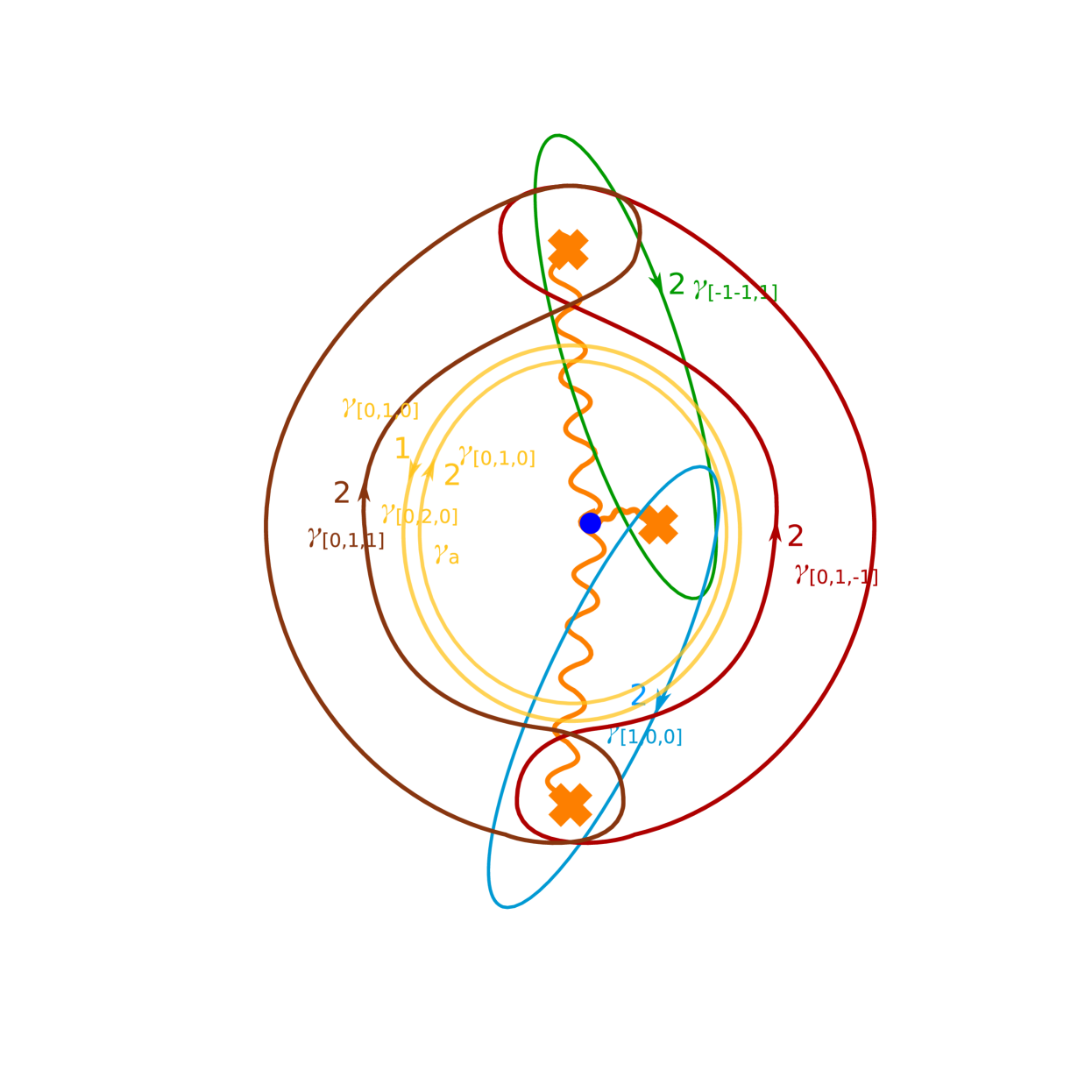
(a)

(b)

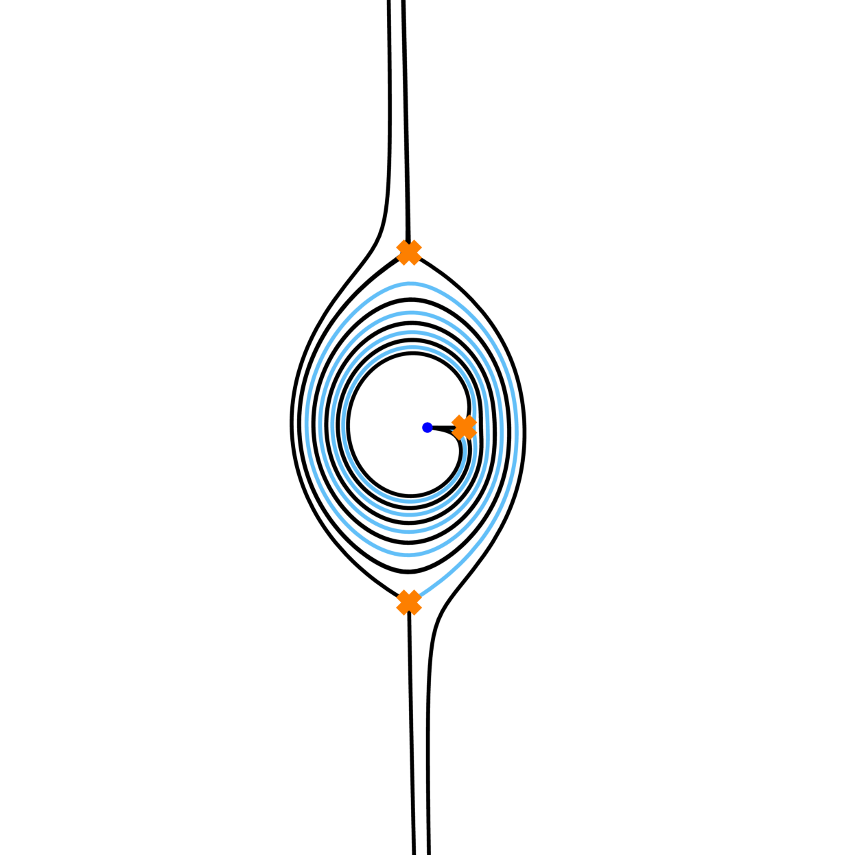
(c)

Figure 4: In 4(a) we plot the lattice charges as loops in the $z$ plane. The yellow double loops is $\gamma_{[0,2,0]}$, while the brown and red loops correspond to $\gamma_{[0,1,1]}$ and $\gamma_{[0,1,-1]}$. The blue loop is $\gamma_{[1,0,0]}$ while the green loop is $\gamma_{[-1,-1,1]}$. Notice that the blue and the green loops are the analytic continuation from the charges in the strong coupling region, see Figure 3. So they maintain their charge labeling. In 4(b) we show $\mathcal{W}^{\vartheta=0,m=0}$ in the $z$ plane. This corresponds to the degenerate spectral network for the BPS vectormultiplet $\gamma_{a}$ and the 2 BPS hypermultiplets $\gamma_{[0,1,1]}$ and $\gamma_{[0,1,-1]}$. There are infinite many BPS hypermultiplets besides $\gamma_{[0,1,1]}$ and $\gamma_{[0,1,-1]}$. We can see this from 4(c) which shows how the spectral network looks when we slightly vary $\vartheta$. This spiraling walls will be more and more less spiraling when $\vartheta$ is varying away from $\vartheta=0$. In this process, there will be infinite saddle connections corresponding to hypermultiplets. These infinite saddle connections correspond to the hypermultiplets $\gamma_{a_{D}}+n\gamma_{a}$ and $\gamma_{[-1,-1,1]}+n\gamma_{a}$, where $n=0,1,...$ is the winding number of the paths inside the ring domain in Figure 4(b).

3.4 Stokes graphs and Borel poles for the local solutions

To discuss Borel summation of the all-orders WKB series, it is useful to first introduce $\vartheta$-Stokes graphs $\mathcal{W}^{\vartheta}$. (If $\vartheta$ is not specified, we assume $\vartheta=\arg(\hbar)$.)

The $\vartheta$-Stokes graph is made of $\vartheta$-Stokes curves on the punctured sphere $C$. Each $\vartheta$-Stokes curve of type $ij$ (where $(i,j)=(1,2)$ or $(2,1)$) is an oriented trajectory starting at a turning point, along which the 1-form $\operatorname{{\rm e}}^{-{\rm i}\vartheta}(Y^{0,(i)}-Y^{0,(j)})\mathrm{d}z$ is real and positive. Stokes graphs are also known as spectral networks, and we will use both names in this paper. Some examples of Stokes graphs appear in Figure 8, Figure 9, Figure 10, Figure 11 below.

The local WKB solutions in each domain of $C\backslash\mathcal{W}^{\vartheta}$ are defined by

$$\psi^{(i)}(z)=\operatorname{{\rm e}}^{\frac{1}{\hbar}\int_{z_{0}}^{z}s(Y^{(i)})(z,\hbar)\mathrm{d}z}.$$ (3.22)

The space of solutions of (3.4) is a 2-dimensional vector space; $\psi^{(1)}$ and $\psi^{(2)}$ form a basis of this vector space in each domain of $C\setminus\mathcal{W}^{\vartheta}$. The solution $\psi^{(i)}$ jumps at a Stokes curve of type $ij$ (while $\psi^{(j)}$ does not jump there.) This jumping is a manifestation of the Stokes phenomenon.

To understand this jumping phenomenon better, note that the Borel summation in (3.22) is only well defined if the Borel transform $\hat{Y}^{(i)}(z,\zeta)$ has no singularities in the $\zeta$-plane along the ray of integration $(0,\operatorname{{\rm e}}^{{\mathrm{i}}\vartheta}\infty)$. The positions of the singularities of $\hat{Y}^{(i)}(z,\zeta)$ in the $\zeta$-plane depend on $z$ (as well as $E$, $\Lambda$, $m$). It is known MR3706198 ; nikolaev2020exact that $\hat{Y}^{(i)}(z,\zeta)$ can only have singularities along the rays $\zeta\in(0,\operatorname{{\rm e}}^{{\mathrm{i}}\vartheta}\infty)$ for specific $\vartheta$, namely those $\vartheta$ such that $z$ lies on a $\vartheta-$Stokes curve of type $ij$. This gives an explanation of the fact that $\psi^{(i)}(z)$ is well defined only for $z$ away from $\vartheta$-Stokes curves of type $ij$.

So far we have described the arguments of singularities of $\hat{Y}^{(i)}$ in the Borel plane, but not their magnitudes. We can make a more precise statement: if $z$ lies on a $\vartheta$-Stokes curve of type $ij$, then $\hat{Y}^{(i)}(z,\zeta)$ has a singularity at

$$\zeta=2\int_{z_{0}}^{z}\lambda\,,$$ (3.23)

where $z_{0}$ is the branch point where the Stokes curve begins. This statement appears in the exact WKB literature: see in particular kawai2005algebraic , where it is explained in terms of the rules for propagation of singularities derived from microlocal analysis.

We made some numerical verifications of this statement in the $SU(2)$ $N_{f}=1$ theory, by choosing a point $z$ and computing Padé approximants to partial sums of the series $\hat{Y}^{(i)}(z,\zeta)$ up to $N$ terms. In the $N\to\infty$ limit, the poles of the Padé approximant lie along curves in the $\zeta$-plane, and the endpoint of each curve is one of the singularities of the true $\hat{Y}^{(i)}(z,\zeta)$. At finite $N$ one sees some approximation to this structure, and can read off an approximation of the position of the desired singularities. We find that they indeed lie at the expected positions (3.23). See Figure 5 and Figure 6 for two examples. In Appendix C.2 we present some similar checks in the pure $SU(2)$ theory.

In terms of quantum field theory, the quantity $2\int_{z_{0}}^{z}\lambda$ has a simple meaning, as follows. We consider the 4d $SU(2)$ $N_{f}=1$ theory coupled to a certain ${\mathcal{N}}=(2,2)$ supersymmetric surface defect $S(z)$, where the parameter $z\in C$ is identified as the coupling of the defect $S(z)$, as discussed in Gaiotto:2009fs ; Gaiotto:2011tf . This surface defect has $2$ vacua corresponding to the sheets $i$, $j$. Then $z$ lies on the $\vartheta$-Stokes curve of type $ij$ exactly if the defect $S(z)$ admits a BPS soliton with phase $\vartheta$ which interpolates from vacuum $i$ to vacuum $j$. In this case $2\int_{z_{0}}^{z}\lambda$ is the central charge of the BPS soliton. In short: singularities of the Borel transform $\hat{Y}^{(i)}(z,\zeta)$ appear at the central charges of BPS solitons in the surface defect theory $S(z)$. The number of singularities depends on the value of $z$; this is the wall-crossing phenomenon for BPS solitons CecottiVafa ; Gaiotto:2011tf .

This proposal is parallel to the proposal of Grassi:2019coc that singularities in the Borel transform of the quantum periods appear at the central charges of BPS particles in the 4d theory. (We will explore that phenomenon in the $SU(2)$ $N_{f}=1$ theory below.) Indeed, taking the conformal limit of the analysis of CecottiVafa ; Gaiotto:2011tf ; gmn , one concludes that Stokes jumps of the local solutions are induced by BPS solitons, in complete parallel to the way that Stokes jumps of the quantum periods are induced by 4d BPS particles.

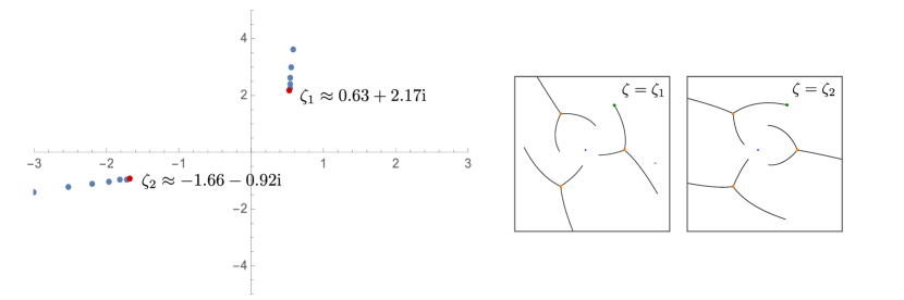
Figure 5: Left: singularities of the Padé-Borel transform of ${Y}^{(2)}$ in (3.7) for $u=0,m=-1/10$, $\Lambda=1$ and $z=\operatorname{{\rm e}}^{{\rm i}}$, with $N=40$ terms in the series. The leading singularities $\zeta_{i}$, marked in red, match well with (3.23); thus as expected they are the central charges of BPS solitons on the surface defect with parameter $z$. (For $Y^{(1)}$ the singularities would be at the opposite points $\zeta=-\zeta_{i}$.) Right: for fixed $\zeta=\zeta_{i}$ we plot a cutoff version of the Stokes graphs with $\vartheta=\arg(\zeta)$, plotting the Stokes curves only up to $|2\int_{z_{0}}^{z}\lambda|=\lvert\zeta\rvert$. As explained around (3.23), the cutoff Stokes curves $\mathcal{W}^{\vartheta=\arg(\zeta_{i})}$ run exactly up to the point $z=\operatorname{{\rm e}}^{\rm i}$, which is plotted as a green dot.

Figure 6: Left: singularities of Padé-Borel transform of $Y^{(2)}$ in (3.7) for $u=2$, $m=0$, $\Lambda=1/5$ and $z=\operatorname{{\rm e}}^{{\rm i}}$, with $N=50$ terms in the series. There are infinitely many poles of $\hat{Y}^{(2)}$, corresponding to the central charges of solitons supported at $z$. Only finitely many of them are visible in our approximation. (Again, for $Y^{(1)}$ the singularities would be at the opposite points $\zeta=-\zeta_{i}$.) Right: cutoff Stokes graphs at $\zeta=\zeta_{1},\zeta_{2},\zeta_{3},\zeta_{4}$, as in Figure 5 above.

3.5 Borel summation for quantum periods

Given $\gamma\in\Gamma$, we define the WKB quantum period $\Pi_{\gamma}^{\rm WKB}(\hbar)$ as the integral of the even part of the WKB series (3.9) along $\gamma$:

$$\Pi_{\gamma}^{\rm WKB}(\hbar)=\frac{1}{\hbar}\sum_{n=0}^{\infty}\Pi_{\gamma}^{n}\hbar^{2n}=\frac{1}{\hbar}\sum_{n=0}^{\infty}\left(\oint_{\gamma}Y^{2n}(z)\mathrm{d}z\right)\hbar^{2n}.$$ (3.24)

In particular,

$$\Pi_{\gamma}^{0}=Z_{\gamma}.$$ (3.25)

We are now ready to define the quantum periods, by Borel summation:

$$\Pi_{\gamma}(\hbar)=\overline{s}\left(\Pi_{\gamma}^{\rm WKB}\right)(\hbar).$$ (3.26)

3.6 The one-loop sign

One might wonder why we do not define the WKB period as the integral of the full WKB series (3.7). The odd part is a total derivative, according to (3.10). Hence the only contribution of the odd part comes from the monodromy of $\log Y_{\mathrm{even}}$ around the contour of integration on $\Sigma$. By expanding the log one sees that this monodromy comes just from the leading term in $Y_{\mathrm{even}}$, i.e. it is the same as the monodromy of $\log\sqrt{P}$. Since $\sqrt{P}$ is single-valued on $\Sigma$, this monodromy is a shift by $2\pi{\mathrm{i}}\omega$ for some $\omega\in\mathbb{Z}$. Thus we have

$$\oint Y_{\rm odd}=-\frac{\hbar}{2}\oint\mathrm{d}\log\sqrt{P}=-\hbar\pi{\rm i}\omega.$$ (3.27)

Including this contribution would lead to an extra sign $\exp\left(\hbar^{-1}\oint Y_{\rm odd}\right)=(-1)^{\omega}$ in the exponentiated WKB series. This sign is subtle, for two distinct reasons:

• It picks up a factor $-1$ when the contour of integration on $\Sigma$ is moved across a branch point, so it is not (quite) a function of a homology class $\gamma\in H_{1}(\Sigma,\mathbb{Z})$.

• It is not coordinate invariant: for a loop which goes around the cylinder, computing in the $z$-plane and the $x$-plane lead to different signs.

For our immediate purpose, it is convenient simply to avoid these issues, by taking only the even part as we did in (3.24); then the resulting $\Pi_{\gamma}$ is canonical, well defined as a function of the homology class (charge) $\gamma$, and additive. However, we will meet this sign again in Section 4.1 below, and we discuss it from a more invariant point of view in Appendix B.

3.7 Padé-Borel computation of quantum periods

The coefficients $\Pi^{n}_{\gamma}$ in (3.26) can be efficiently computed by using the differential operator technique, parallel to Grassi:2019coc ; huangNS ; Huang:2014nwa . We first note that the $Y^{2n}(z,u,m)\mathrm{d}z$ term can be expressed as

$$Y^{2n}(z,u,m)\mathrm{d}z=b_{0}^{n}Y^{0}(z,u,m)\mathrm{d}z+b_{1}^{n}\frac{\partial Y^{0}(z,u,m)}{\partial m}\mathrm{d}z+b_{2}^{n}\frac{\partial Y^{0}(z,u,m)}{\partial u}\mathrm{d}z+\mathrm{d}(\cdots)$$ (3.28)

where $\mathrm{d}(\cdots)$ denotes a total derivative term in $z$. Therefore $\Pi^{n}_{\gamma}$ satisfies

$$\Pi^{n}_{\gamma}(z,u,m)=b_{0}^{n}\Pi^{0}_{\gamma}(z,u,m)+b_{1}^{n}\frac{\partial\Pi^{0}_{\gamma}(z,u,m)}{\partial m}+b_{2}^{n}\frac{\partial\Pi^{0}_{\gamma}(z,u,m)}{\partial u}.$$ (3.29)

We also emphasize that the quantum period for the flavor charge $\Pi_{\gamma_{[0,0,1]}}$ is not subject to quantum corrections, as discussed for instance in Huang:2014nwa (see also Appendix A for a direct computation). In other words,

$$\Pi_{\gamma_{[0,0,1]}}(\hbar)=\frac{Z_{\gamma_{[0,0,1]}}}{\hbar}=-\frac{2\pi m}{\hbar}\,.$$ (3.30)

In particular $\Pi^{n}_{\gamma_{f}}=0$, $\forall n>0$, which implies the constraints

$$b_{1}^{n}=-mb_{0}^{n}\,.$$ (3.31)

	$i=0$	$i=1$	$i=2$
$b_{i}^{1}$	$\frac{25}{6734}$	$\frac{5}{13468}$	$\frac{-3371}{80808}$
$b_{i}^{2}$	$\frac{121523975}{196306106724}$	$\frac{24304795}{392612213448}$	$-\frac{1738734625}{1046965902528}$
$b_{i}^{3}$	$\frac{14649990947544027025}{1744761644092944719424}$	$\frac{2929998189508805405}{3489523288185889438848}$	$-\frac{2245318130362254755}{2326348858790592959232}$
$b_{i}^{4}$	$\frac{1156307121570685086685480765}{79119280552841605513208588544}$	$\frac{231261424314137017337096153}{158238561105683211026417177088}$	$-\frac{1685881772274283567722957525}{140656498760607298690148601856}$

Table 2: The first few $b_{i}^{n}$, for $u=0$, $m=-1/10$, $\Lambda=1$.

Given the form of the relation (3.29) it is relatively straightforward to compute the coefficients $b_{i}^{n}$ up to $n=80$, at any particular point $(\Lambda,m,u)$; we show samples of the first few $b_{i}^{n}$ in Table 2. Then we compute the three quantities $\Pi_{\gamma}^{0}$, $\partial_{u}\Pi_{\gamma}^{0}$ and $\partial_{m}\Pi_{\gamma}^{0}$ by direct numerical integration. Thus we obtain $80$ terms of the series $\Pi_{\gamma}^{\mathrm{WKB}}$. Then following the same Padé-Borel summation technique discussed in Section 3.4, we get the approximate quantum period $\Pi^{\rm PB}_{\gamma}$. In this way one can get many digits of precision; see Table 1 for some sample results.

Let us comment briefly on the singularities of the Borel transform $\hat{\Pi}_{\gamma}$. As predicted in Grassi:2019coc , $\hat{\Pi}_{\gamma}$ is expected to have singularities at $\zeta=Z_{\gamma^{\prime}}$ when $\gamma^{\prime}$ is the charge of a BPS particle existing in the theory at the particular point in moduli space that we are studying, and $\langle\gamma,\gamma^{\prime}\rangle\neq 0$. In Figure 7 we show numerical checks of this phenomenon at strong and weak coupling; we indeed find the poles at the expected places. These singularities are responsible for the fact that $\Pi_{\gamma}^{\mathrm{PB}}$ is only piecewise analytic, as we reviewed in Section 2.

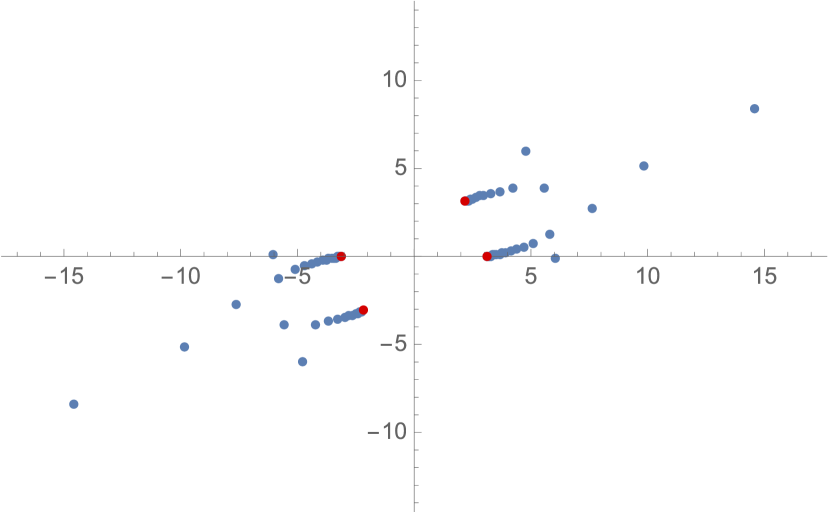
(a)

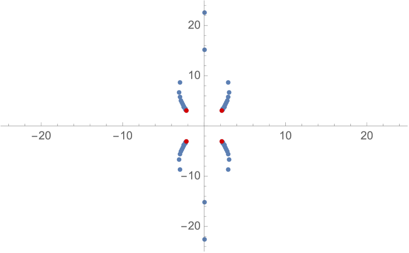
(b)

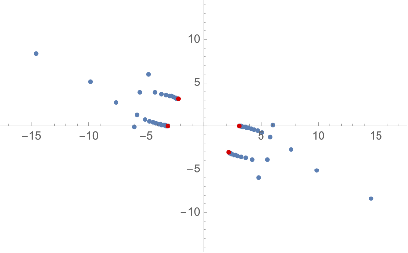
(c)

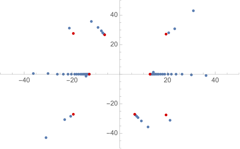
(d)

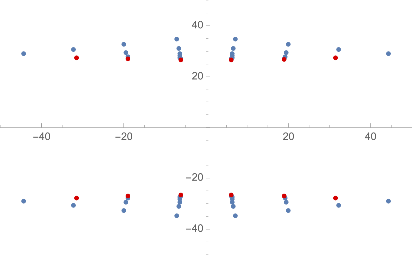
(e)

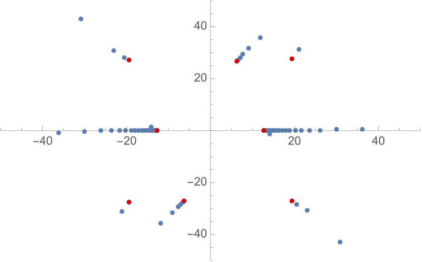
(f)

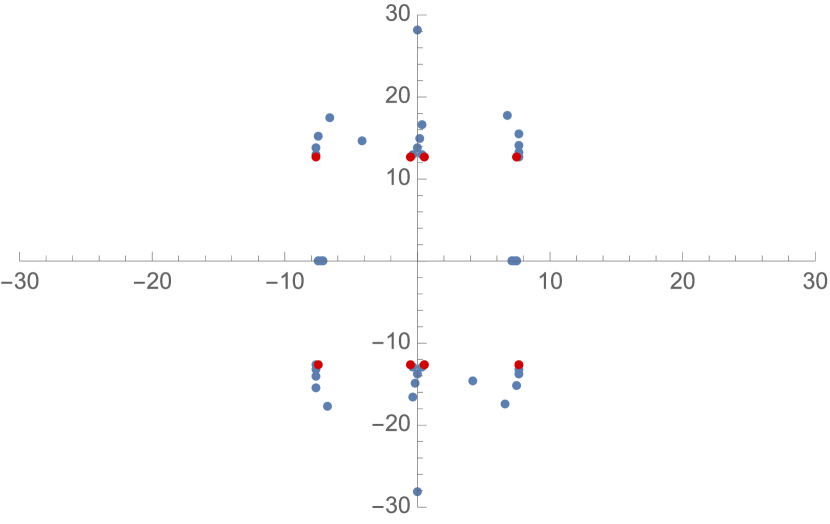
(g)

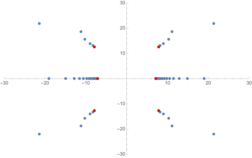
(h)

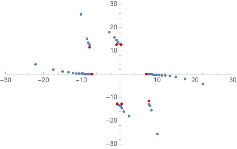
(i)

Figure 7: Poles of the Padé-Borel transform for various quantum periods. The first row shows the poles for $\Pi_{\gamma_{[1,0,0]}}$ (left), $\Pi_{\gamma_{[0,1,1]}}$(center) and $\Pi_{\gamma_{[-1-1,1]}}$ (right) in strong coupling region at $u=0$, $m=-1/10$ and $\Lambda=1$. The second row shows the poles for $\Pi_{\gamma_{[1,0,0]}}$(left), $\Pi_{\gamma_{[0,2,0]}}$(center) and $\Pi_{\gamma_{[-1,-1,1]}}$ (right) in weak coupling region for $u=2$, $m=0$ and $\Lambda=1/5$. The third row shows the poles for $\Pi_{\gamma_{[1,0,0]}}$(left), $\Pi_{\gamma_{[0,2,0]}}$(center) and $\Pi_{\gamma_{[-1,-1,1]}}$ (right) in weak coupling region for $u=-2$, $m=1/10$ and $\Lambda=1$. The first poles in each accumulated series are denoted by red dots. The position of such poles correspond approximately to the central charges of BPS states with non-zero intersection numbers w.r.t. the charge $\gamma_{[-,-,-]}$ under consideration.

4 Computation by small sections

4.1 Rules for writing down Wronskians

In this chapter we explain how to use Wronskians of local solutions of (1.3) to compute quantum periods, following a general formalism laid out in Gaiotto:2009hg ; Hollands:2019wbr .

The basic ingredients needed are:

1. Three solutions $\psi_{1}$, $\psi_{2}$ and $\psi_{3}$ of (1.3), which decay exponentially along three paths approaching the irregular singularities of the equation at $z=0$, $z=\infty$.

2. The monodromy operator $M$ giving evolution of the solutions of (1.3) under $x\to x+2\pi{\mathrm{i}}$, and its eigenfunctions $\psi_{4}$, $\psi_{5}$.

Below we give some brief insight into what $\psi_{1}$, $\psi_{2}$, $\psi_{3}$, $\psi_{4}$, $\psi_{5}$ are, and why we use them in our calculation.

4.1.1 Global structure of the Stokes graph

We need to discuss a bit about the global structure of the Stokes graph (see e.g. Gaiotto:2009hg for more).

Recall that the Stokes curves of type $ij$ are examples of WKB curves of type $ij$, i.e. curves along which $\operatorname{{\rm e}}^{-{\rm i}\vartheta}(Y^{0,(i)}-Y^{0,(j)})\mathrm{d}z$ is real and positive. When any WKB curve of type $ij$ approaches an irregular singularity, it asymptotes to one of the distinguished Stokes directions around the singularity with the same implicit label $ij$. In a local coordinate $\tilde{z}$, each Stokes direction is a ray going into $\tilde{z}=0$, characterized by the property that at $\tilde{z}\to 0$ along the ray

$$\arg\left(\int^{\tilde{z}}_{\tilde{z}_{0}}(Y^{0,(i)}-Y^{0,(j)})\mathrm{d}\tilde{z}^{\prime}\right)\to\vartheta\text{ as }\tilde{z}\rightarrow 0.$$ (4.1)

To determine these directions explicitly it is sufficient to consider the leading-order behavior of $(Y^{0,(i)}-Y^{0,(j)})$. Moreover, because the integral diverges as $\tilde{z}\to 0$ we see that the choice of $\tilde{z}_{0}$ is unimportant. We will show examples shortly, and see that in the $SU(2)$ $N_{f}=1$ theory there is one Stokes direction going into $z=0$ and two going into $z=\infty$.

We can also consider generic WKB curves; each such curve is determined given a point $z\in C\backslash\mathcal{W}$ it goes through. Generic WKB curves never intersect each other, nor do they intersect the Stokes curves; the Stokes curves and generic WKB curves together make up a foliation of the Riemann surface $C$.

For generic $\vartheta$, following any generic WKB curve in either direction leads asymptotically to one of the Stokes directions around one of the irregular singularities, and likewise for following a Stokes curve in the forward direction. For special $\vartheta$, $\vartheta=\arg(-Z_{\gamma_{\rm BPS}})$ with $\gamma_{\rm BPS}$ the charge of a BPS particle, there are two other possibilities. First, we can have a saddle connection, a Stokes curve connecting two turning points; this corresponds to a BPS hypermultiplet. Explicit examples are shown in 4(b) and 4(c). Second, we can have a ring domain, a 1-parameter family of closed WKB curves; this corresponds to a BPS vectormultiplet. A ring domain has two boundaries; each boundary is generically a single Stokes curve emanating from a turning point and returning to the same turning point, but in special cases (such as the $m=0$ case in 4(b)) it can be broken into multiple saddle connections between multiple turning points.

4.1.2 Exponentially decaying solutions

Following the discussion above, in each Stokes direction going into a singularity, we get for free a corresponding exponentially decaying solution (up to a constant). Recall that the ansatz we use in the WKB method is

$$\psi(z)=\operatorname{{\rm e}}^{\hbar^{-1}\int_{z_{0}}^{z}Y(z)\mathrm{d}z}.$$ (4.2)

Now suppose $z$ approaches an irregular singularity along a Stokes direction with label $ij$. Then we have

$$\frac{\psi^{(j)}}{\psi^{(i)}}\sim\operatorname{{\rm e}}^{\hbar^{-1}\left(\int_{z_{0}}^{z}(Y^{0,(j)}(z)-Y^{0,(i)}(z))\mathrm{d}z\right)}\to\operatorname{{\rm e}}^{\frac{-\infty\operatorname{{\rm e}}^{{\rm i}\vartheta}}{\hbar}}.$$ (4.3)

Since we require $\rm Re(\operatorname{{\rm e}}^{-{\rm i}\vartheta}\hbar)>0$, $\psi^{(j)}$ is exponentially small compared to $\psi^{(i)}$ when $z$ approaches the singularity. Moreover, since $Y^{(i)}=-Y^{(j)}$ we can also write this ratio as

$$\operatorname{{\rm e}}^{\hbar^{-1}\int_{z_{0}}^{z}(Y^{0,(j)}(z)-Y^{0,(i)}(z))\mathrm{d}z}=\operatorname{{\rm e}}^{\hbar^{-1}\int_{z_{0}}^{z}2Y^{0,(j)}(z)\mathrm{d}z}\sim{\psi^{(j)}}^{2}.$$ (4.4)

Thus $\psi^{(j)}$ is exponentially decaying as $z$ goes into the singularity along a Stokes direction with label $ij$.

We look at the two singularities separately:

1. When $z\rightarrow 0$, $\int Y^{0,(i)}-Y^{0,(j)}\mathrm{d}z\sim\pm\frac{\Lambda}{2z^{1/2}}$. Given a phase $\vartheta$, we have 1 Stokes direction. Figure 8 is an example at $\vartheta=0$; then the Stokes direction at $z=0$ is $0^{+}$ with label $12$. The exponentially decaying solution along Stokes direction is

   $$\psi_{1}\equiv\psi^{(2)}=\operatorname{{\rm e}}^{\hbar^{-1}\int_{z_{0}}^{z}Y^{(2)}\mathrm{d}z}.$$ (4.5)

2. When $z\rightarrow\infty$, we use $\tilde{z}=\frac{1}{z}$, and then $\int Y^{0,(i)}-Y^{0,(j)}\mathrm{d}z\sim\pm\frac{{\rm i}\Lambda}{\tilde{z}}$. Given a phase $\vartheta$, there are 2 Stokes directions with opposite labels. In Figure 8, which is at $\vartheta=0$, the Stokes directions at $z=\infty$ are $\infty\operatorname{{\rm e}}^{\pi{\rm i}/2}$ with label $12$ and $\infty\operatorname{{\rm e}}^{-\pi{\rm i}/2}$ with label $21$. The exponentially decaying solution along Stokes direction $21$ is

   $$\psi_{2}\equiv\psi^{(1)}=\operatorname{{\rm e}}^{\hbar^{-1}\int_{z_{0}}^{z}Y^{(1)}\mathrm{d}z},$$ (4.6)

   and the exponentially decaying solution along Stokes direction $12$ is

   $$\psi_{3}\equiv\psi^{(2)}=\operatorname{{\rm e}}^{\hbar^{-1}\int_{z_{0}}^{z}Y^{(2)}\mathrm{d}z}.$$ (4.7)

Now suppose we look at a generic WKB curve. In one direction it goes into a Stokes direction with label $ij$, and in the other direction it goes into a Stokes direction with label $ji$. Thus the two WKB solutions $\psi^{(i)}$, $\psi^{(j)}$ along this curve can also be described as the exponentially decaying solutions in these two Stokes directions.

The Stokes graph $\mathcal{W}^{\vartheta}$ separates $C\backslash\mathcal{W}^{\vartheta}$ into domains. In each domain, all generic WKB curves run between the same pair of asymptotic Stokes directions. Thus the basis of exponentially decaying solutions which we obtain in a given domain is the same no matter which generic WKB curve we consider. When we move across a Stokes curve to a different domain, one or both of the asymptotic Stokes directions along generic WKB curves changes, and thus the basis of exponentially decaying solutions jumps. This is consistent with the fact we reviewed in Section 3.4, that the basis of solutions $\psi^{(1)}$, $\psi^{(2)}$ is well defined up to constant multiple in each domain, and jumps (due to the presence of singularities in the Borel plane) when we cross a Stokes curve from one domain to another.

In some cases a generic WKB curve goes to the same asymptotic Stokes direction at both ends. This might seem like a contradiction: there is only one exponentially decaying solution at that Stokes direction, so how will we get a basis of solutions from exponentially decaying solutions along this WKB curve? The resolution is that we need to be careful about the global monodromy: when we speak of the two-dimensional space of global solutions of the equation, we really mean the space of solutions on the complement of some branch cut (“monodromy cut”) in the $z$-plane. When we transport a solution across this cut we transform it by the action of the monodromy $M$ or $M^{-1}$. We will see examples below.

Inside ring domains, the Stokes curves do not go to any irregular singularity. Thus we cannot find a basis of solutions there using our exponential-decay prescription. Instead, the appropriate basis consists of the eigenfunctions of the monodromy around the ring, as described e.g. in Hollands:2013qza .

As we have just reviewed, in each domain of $C\setminus\mathcal{W}$ we have a distinguished pair of solutions determined up to scalar multiple. We will call the exponentially decaying solutions approaching singularities $\psi_{1}$, $\psi_{2}$ and $\psi_{3}$ as indicated in (4.5), (4.6), (4.7). Then, see Figure 8, Figure 9, Figure 10, Figure 11 for some examples of explicit local bases.

Some convenient rules for writing down the local bases of solutions in all domains are Hollands:2019wbr :

1. We use the notation $(\psi,\psi^{\prime})$ to represent a local basis of solutions $(\psi^{(1)},\psi^{(2)})$ labeled by the two sheets of the covering $\Sigma\to C$. $\psi$ and $\psi^{\prime}$ are swapped when crossing a branch cut:

   $$(\psi,\psi^{\prime})\rightarrow(\psi^{\prime},\psi)$$ (4.8)

2. We choose a monodromy cut for the differential equation as discussed above, and when we cross this cut, the basis gains a factor of the monodromy matrix $M$.

   $$(\psi,\psi^{\prime})\rightarrow(M\psi,M\psi^{\prime})$$ (4.9)

3. When we cross a Stokes curve of type $ij$, the solution $\psi^{(j)}$ is unchanged, while $\psi^{(i)}$ generally changes.

   (This can be understood as: shifting the exponentially growing solution by a multiple of the exponentially decaying solution gives another exponentially growing solution. But we will not use this point of view explicitly, and will simply treat $\psi^{(i)}$ on the two sides of the wall as different solutions.)

4. When we cross a double wall, both $\psi^{(1)}$ and $\psi^{(2)}$ generally change.

5. In a ring domain, the local basis of solutions is not constructed directly from the exponentially decaying solutions; rather they are eigenfunctions of the monodromy matrix $M$. (Thus, strictly speaking, they are not single-valued solutions on the ring domain, but rather on the complement of a monodromy cut.)

In terms of these local bases, the quantum period associated to a cycle $\gamma$ is obtained as a product of factors as follows. Let $[\psi,\psi^{\prime}]$ denote the Wronskian of the two solutions $\psi$ and $\psi^{\prime}$.

1. When $\gamma$ crosses a single Stokes curve of type $ij$ on sheet $i$, from side $L$ to $R$, add a factor $\frac{[\psi_{i}^{L},\psi_{j}^{L}]}{[\psi_{i}^{R},\psi_{j}^{L}]}$ to the product.

2. When $\gamma$ crosses a double Stokes curve on sheet $i$, add a factor $\sqrt{\frac{[\psi_{i}^{L},\psi_{j}^{L}]}{[\psi_{i}^{R},\psi_{j}^{R}]}\frac{[\psi_{i}^{L},\psi_{j}^{R}]}{[\psi_{i}^{R},\psi_{j}^{L}]}}$ to the product. (This factor is ambiguous as written, because we have not specified a branch of the square root. This sign can in principle be determined following a rule given in Hollands:2019wbr , but this rule is cumbersome in practice; in this paper we will not try to implement it, and just live with this sign ambiguity in cases involving double Stokes curves. All formulas in this paper which involve a square root of a product of Wronskians have to be understood as having this sign ambiguity; in numerical comparisons we just fix the sign by hand when necessary.)

3. When $\gamma$ crosses a monodromy cut in a ring domain, add a factor $\mu$ or $\frac{1}{\mu}$ to the product, where $\mu$, $\frac{1}{\mu}$ denote the eigenvalues of the monodromy operator $M$.

4. We include an overall sign factor $\exp(-\frac{1}{4}\oint_{\gamma}\frac{\mathrm{d}P}{P})$, where $P(x)$ is the potential in the cylinder coordinate, given in (3.2). (This factor was not included in the rules in Hollands:2019wbr ; we saw it in Section 3.6, and we discuss it more in Appendix B.)

Combining all factors as described above when going along some loop $\gamma$, we obtain the Wronskian expression $\mathcal{X}_{\gamma}^{\rm SS,\vartheta}$. The result only depends on the homology class $\gamma$, although the individual factors may well depend on the precise choice of representative.

4.2 Quantum periods in strong coupling region

As an example we can choose the parameters to be $u=0$, $m=-1/10$ and $\Lambda=1$. The corresponding spectral network $\mathcal{W}^{\vartheta=0}$ is shown in Figure 8. By applying the rules given in Section 4.1 we obtain the following Wronskian expressions for the quantum periods:

$$\mathcal{X}^{\rm SS,\vartheta=0}_{\gamma_{[0,1,1]}}=-\frac{[\psi_{3},\psi_{1}]}{[M\psi_{1},\psi_{1}]}\frac{[\psi_{1},\psi_{2}]}{[M^{-1}\psi_{3},\psi_{2}]}\,,$$ (4.10)

$$\mathcal{X}^{\rm SS,\vartheta=0}_{\gamma_{[-1,-1,1]}}=\frac{[\psi_{2},\psi_{3}]}{[\psi_{2},\psi_{1}]}\sqrt{\frac{[M\psi_{1},\psi_{1}]}{[\psi_{2},M^{-1}\psi_{3}]}\frac{[M\psi_{2},\psi_{1}]}{[M\psi_{1},\psi_{3}]}}\,,$$ (4.11)

$$\mathcal{X}^{\rm SS,\vartheta=0}_{\gamma_{[1,0,0]}}=\frac{[\psi_{3},\psi_{2}]}{[\psi_{3},\psi_{1}]}\sqrt{\frac{[\psi_{1},M\psi_{1}]}{[M^{-1}\psi_{3},\psi_{2}]}\frac{[\psi_{3},M\psi_{1}]}{[\psi_{1},M\psi_{2}]}}\,.$$ (4.12)

For completeness we also show the Wronskian expression for the period corresponding to flavor mass:

$$\mathcal{X}^{{\rm SS},\vartheta=0}_{\gamma_{[0,0,1]}}=-\frac{[\psi_{3},\psi_{2}]}{[M^{-1}\psi_{3},\psi_{2}]}=\operatorname{{\rm e}}^{\frac{-2\pi m}{\hbar}}\,.$$ (4.13)

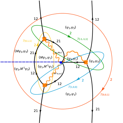
Figure 8: $\mathcal{W}^{\vartheta=0}$ for $u=0,\ m=-1/10,\ \Lambda=1$ in the strong coupling region. Blue dotted line is the monodromy cut. The local basis of solutions for each domain is listed as $(\psi^{(1)},\psi^{(2)})$.

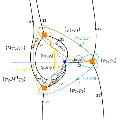
Figure 9: Spectral network and local bases of solutions corresponding to $\vartheta=\arg(1+\frac{1}{10}{\rm i})$, with other parameters as in Figure 8.

Alternatively we can consider $\mathcal{W}^{\vartheta=\arg(1+\frac{{\rm i}}{10})}$ as shown in Figure 9. The resulting expressions are

$$\mathcal{X}^{{\rm SS},\vartheta=\arg(1+\frac{{\rm i}}{10})}_{\gamma_{[0,1,1]}}=-\frac{[\psi_{3},\psi_{1}]}{[M\psi_{1},\psi_{1}]}\frac{[\psi_{1},\psi_{2}]}{[M^{-1}\psi_{3},\psi_{2}]}\,,$$ (4.14)

$$\mathcal{X}^{{\rm SS},\vartheta=\arg(1+\frac{{\rm i}}{10})}_{\gamma_{[-1,-1,1]}}=-\frac{[\psi_{1},M\psi_{1}]}{[\psi_{3},M\psi_{1}]}\frac{[\psi_{3},\psi_{2}]}{[\psi_{1},\psi_{2}]}\,,$$ (4.15)

$$\mathcal{X}^{{\rm SS},\vartheta=\arg(1+\frac{{\rm i}}{10})}_{\gamma_{[1,0,0]}}=-\frac{[\psi_{3},\psi_{2}]}{[M^{-1}\psi_{3},\psi_{2}]}\frac{[M^{-1}\psi_{3},\psi_{1}]}{[\psi_{3},\psi_{1}]}\,.$$ (4.16)

These periods are related by

$$\frac{\mathcal{X}^{{\rm SS},\vartheta=\arg(1+\frac{{\rm i}}{10})}_{\gamma_{[-1,-1,1]}}}{\mathcal{X}^{\rm SS,\vartheta=0}_{\gamma_{[-1,-1,1]}}}={} \sqrt{\frac{[M\psi_{1},\psi_{1}]}{[M\psi_{1},\psi_{3}]}\frac{[M\psi_{2},\psi_{3}]}{[M\psi_{2},\psi_{1}]}}$$ (4.17)

$$={} \frac{1}{\sqrt{1-\frac{[\psi_{1},\psi_{3}][\psi_{2},\psi_{1}]}{[\psi_{1},M\psi_{1}][\psi_{2},M^{-1}\psi_{3}]}}}$$

$$={} (1+\mathcal{X}^{{\rm SS},\vartheta=\arg(1+\frac{{\rm i}}{10})}_{\gamma_{[0,1,1]}})^{-\frac{1}{2}}=(1+\mathcal{X}^{{\rm SS},\vartheta=\arg(0)}_{\gamma_{[0,1,1]}})^{-\frac{1}{2}}.$$

This relation is precisely the KS transformation (2.1)-(2.3) corresponding to the hypermultiplet of charge $\gamma_{[0,1,1]}$ in the spectrum.

We evaluated these Wronskians numerically; some results are shown in Table 1.

4.3 Quantum periods in weak coupling region

Now let us consider the point $u=2,\ m=0,\ \Lambda=1/5$ in the weak coupling region. We use the spectral network $\mathcal{W}^{\vartheta=0}$ shown in Figure 10. Again using the rules of Section 4.1, we obtain Wronskian expressions for the quantum periods:

$$\mathcal{X}^{\rm SS,\vartheta=0}_{\gamma_{[-1,-1,1]}}=-\sqrt{-\frac{1}{\mu}}\frac{[\psi_{1},\psi_{4}]}{[\psi_{1},\psi_{5}]}\sqrt{\frac{[\psi_{3},\psi_{2}][\psi_{3},\psi_{5}][\psi_{5},\psi_{2}]}{[\psi_{4},\psi_{2}][\psi_{3},M\psi_{2}][\psi_{3},\psi_{4}]}}\,,$$ (4.18)

$$\mathcal{X}^{\rm SS,\vartheta=0}_{\gamma_{[1,0,0]}}=\sqrt{-\frac{1}{\mu}}\frac{[\psi_{1},\psi_{5}]}{[\psi_{1},\psi_{4}]}\sqrt{\frac{[\psi_{3},\psi_{2}][\psi_{4},\psi_{2}][\psi_{3},\psi_{4}]}{[\psi_{3},M\psi_{2}][\psi_{3},\psi_{5}][\psi_{5},\psi_{2}]}}\,,$$ (4.19)

$$\mathcal{X}^{\rm SS,\vartheta=0}_{\gamma_{[0,1,0]}}=\mu\,,$$ (4.20)

where $\mu$ is the eigenvalue of the monodromy matrix $M$ chosen by comparing with the same quantum period gotten in other method. $\psi_{4}$ and $\psi_{5}$ are eigenfunctions of $M$ such that $M\psi_{4}=\frac{1}{\mu}\psi_{4}$ and $M\psi_{5}=\mu\psi_{5}$. For completeness, we also show

$$\mathcal{X}^{{\rm SS},\vartheta=0}_{\gamma_{[0,0,1]}}=-\frac{[\psi_{3},\psi_{2}]}{[M^{-1}\psi_{3},\psi_{2}]}\,.$$ (4.21)

(a)

(b)

Figure 10: The spectral network $\mathcal{W}^{\vartheta=0}$ for $u=2$, $m=0$, $\Lambda=1/5$ in the weak coupling region. The blue dotted line is the monodromy cut. The local basis of solutions in each domain is listed as $(\psi^{(1)},\psi^{(2)})$. The two figures are identical except that we show different bases for the charge lattice.

For later convenience we also show the $\mathcal{X}_{\gamma}$ for a few other charges:

$$\mathcal{X}^{{\rm SS},\vartheta=0}_{\gamma_{[0,1,-1]}}=-\mu\frac{[M^{-1}\psi_{3},\psi_{2}]}{[\psi_{3},\psi_{2}]}=\mu\frac{1}{\mathcal{X}^{{\rm SS},\vartheta=0}_{\gamma_{[0,0,1]}}}=\mu\operatorname{{\rm e}}^{\frac{2\pi m}{\hbar}}\,,$$ (4.22)

$$\mathcal{X}^{{\rm SS},\vartheta=0}_{\gamma_{[0,1,1]}}=-\mu\frac{[\psi_{3},\psi_{2}]}{[M^{-1}\psi_{3},\psi_{2}]}=\mu\mathcal{X}^{{\rm SS},\vartheta=0}_{\gamma_{[0,0,1]}}=\mu\operatorname{{\rm e}}^{-\frac{2\pi m}{\hbar}}\,.$$ (4.23)

Notice that if $m=0$,

$$\mathcal{X}^{{\rm SS},\vartheta=0}_{\gamma_{[0,1,-1]}}=\mathcal{X}^{{\rm SS},\vartheta=0}_{\gamma_{[0,1,1]}}=\mathcal{X}^{{\rm SS},\vartheta=0}_{\gamma_{[0,1,0]}}=\mu.$$ (4.24)

4.4 Quantization condition

In this section we study the quantization condition for the operator (1.3), in the particular situation where the potential is real, convex and confining along some path in the $z$-plane. In this case the bound states correspond to solutions decaying exponentially when approaching both ends of the path. Such a solution exists when the solutions decaying on Stokes directions at the two ends of the path are linearly dependent. We will see below that the resulting quantization condition for the energy spectrum takes the simple form

$$\mathcal{X}_{\gamma_{[1,0,0]}}=-1.$$ (4.25)

As an example we take

$$\hbar>0,\quad m=\frac{{\rm i}}{10},\quad\Lambda=\operatorname{{\rm e}}^{-\frac{\pi{\rm i}}{6}}\,.$$ (4.26)

The corresponding spectral network and local solutions for $\mathcal{W}^{\vartheta=0}$ at $u=2$ are shown in Figure 11. More generally, keeping $\Lambda$ and $m$ fixed, we allow $u$ to vary in a range on $\mathbb{R}$ containing $u=2$ so long as the spectral network maintains the same topology. The locus we are considering is in the weak coupling region and at the special phase $\vartheta=0$, which is the phase of the central charge of the BPS vectormultiplet; thus we see a ring domain in Figure 11.

With the parameters (4.26), the Schrödinger equation (1.3) becomes

$$\left(-\hbar^{2}\partial_{x}^{2}+(\frac{\operatorname{{\rm e}}^{-\frac{\pi{\rm i}}{3}}\operatorname{{\rm e}}^{-x}}{2}+\frac{\operatorname{{\rm e}}^{\frac{\pi{\rm i}}{3}}\operatorname{{\rm e}}^{x}}{5}-\operatorname{{\rm e}}^{-\frac{\pi{\rm i}}{3}}\operatorname{{\rm e}}^{2x})-2u\right)\psi(x)=0.$$ (4.27)

If we choose a path parametrized by

$$x=t-\frac{\pi{\rm i}}{3}\quad t\in\mathbb{R}\,,$$ (4.28)

then (4.27) becomes

$$\left(-\hbar^{2}\partial_{t}^{2}+(\frac{\operatorname{{\rm e}}^{-t}}{2}+\frac{\operatorname{{\rm e}}^{t}}{5}+\operatorname{{\rm e}}^{2t})-2u\right)\psi(t)=0,$$ (4.29)

with real convex confining potential along $t\in\mathbb{R}$. Bound states are solutions $\psi(t)$ decaying as $t\rightarrow\pm\infty$. The corresponding path in the $z$ plane is

$$z=\operatorname{{\rm e}}^{x}=\operatorname{{\rm e}}^{-\frac{\pi{\rm i}}{3}}\operatorname{{\rm e}}^{t}.$$ (4.30)

Hence a bound state corresponds to a solution in the $z$-plane which decays exponentially as we approach $z=\operatorname{{\rm e}}^{-\frac{\pi{\rm i}}{3}}\operatorname{{\rm e}}^{\infty}=\operatorname{{\rm e}}^{-\frac{\pi{\rm i}}{3}}\infty$ and $z=\operatorname{{\rm e}}^{\frac{-\pi{\rm i}}{3}}\operatorname{{\rm e}}^{-\infty}=\operatorname{{\rm e}}^{\frac{-\pi{\rm i}}{3}}0$. In the labeling shown in Figure 11, the decaying solutions in these two directions are named $\psi_{2}$ and $\psi_{1}$ respectively; thus the bound state condition is that $\psi_{1}$ and $\psi_{2}$ are linearly dependent.

The Wronskian expressions for the quantum periods in this parameter chamber, again obtained by the rules of Section 4.1, are

$$\mathcal{X}^{\rm SS,\vartheta=0}_{\gamma_{[0,1,0]}}(E,\Lambda=\operatorname{{\rm e}}^{-{\rm i}\pi/6},m={\frac{{\rm i}}{10}},\hbar)=\mu\,,$$ (4.31)

$$\mathcal{X}^{\rm SS,\vartheta=0}_{\gamma_{[1,0,0]}}(E,\Lambda=\operatorname{{\rm e}}^{-{\rm i}\pi/6},m={\frac{{\rm i}}{10}},\hbar)=\frac{[\psi_{1},\psi_{5}][\psi_{4},\psi_{2}]}{[\psi_{4},\psi_{1}][\psi_{5},\psi_{2}]}\,.$$ (4.32)

Bound states exist when $\psi_{1}=\lambda\psi_{2}$. Substituting this condition in (4.32) we see that it implies

$$\mathcal{X}^{\rm SS,\vartheta=0}_{\gamma_{[1,0,0]}}(E,\Lambda=\operatorname{{\rm e}}^{-{\rm i}\pi/6},m={\frac{{\rm i}}{10}},\hbar)=-1\,.$$ (4.33)

This is the exact quantization condition. It has a discrete set of solutions $\{E_{n}\}_{n\geq 0}$, which give the bound state energies for (4.29).

For completeness, we also show another quantum period at this point (although this one does not participate in the quantization condition):

$$\mathcal{X}^{\rm SS,\vartheta=0}_{\gamma_{[-1,-1,1]}}(E,\Lambda=\operatorname{{\rm e}}^{-{\rm i}\pi/6},m={\frac{{\rm i}}{10}},\hbar) =-\frac{[\psi_{4},\psi_{1}]}{[\psi_{1},\psi_{5}]}\frac{[\psi_{5},M\psi_{2}]}{[\psi_{4},\psi_{2}]}\frac{[\psi_{3},\psi_{2}]}{[\psi_{3},M\psi_{2}]}\,,$$ (4.34)

$$=-\frac{1}{\mu}\frac{[\psi_{4},\psi_{1}]}{[\psi_{1},\psi_{5}]}\frac{[\psi_{5},\psi_{2}]}{[\psi_{4},\psi_{2}]}\frac{[\psi_{3},\psi_{2}]}{[\psi_{3},M\psi_{2}]}\,.$$

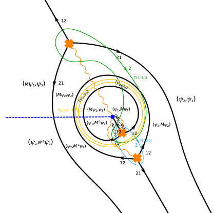
Figure 11: $\mathcal{W}^{\vartheta=0}$ at $u=2,\ m={\rm i}/10,\ \Lambda=\operatorname{{\rm e}}^{-{\rm i}\pi/6}$. Decaying solutions are along $\mathbb{R}\operatorname{{\rm e}}^{-\pi{\rm i}/3}$ approaching $\operatorname{{\rm e}}^{-\pi{\rm i}/3}\infty$, $\operatorname{{\rm e}}^{-\pi{\rm i}/3}0$ and $\operatorname{{\rm e}}^{2\pi{\rm i}/3}\infty$.

5 TBAs in the strong coupling region

5.1 The GMN TBA

In this section we briefly review the TBA of Gaiotto:2014bza (conformal limit of the GMN TBA gmn ; Gaiotto:2009hg ), focusing on the example of the $SU(2)$ $N_{f}=1$ theory. As we will see, this system of integral equations provides us with another way to compute quantum periods.

We consider spectral coordinates $\mathcal{X}_{\gamma}^{\rm TBA}$ obeying

$$\mathcal{X}_{\gamma}^{\rm TBA}(\hbar)=\exp\left(\frac{Z_{\gamma}}{\hbar}+\frac{1}{4\pi{\rm i}}\sum_{\gamma^{\prime}\in\Gamma}\Omega(\gamma^{\prime},u)\langle\gamma,\gamma^{\prime}\rangle\mathcal{I}_{\gamma^{\prime}}(\hbar)\right),$$ (5.1)

where $\Omega(\gamma^{\prime},u)$ denotes the BPS index of BPS states with charge $\gamma^{\prime}$ and

$$\mathcal{I}_{\gamma}(\hbar)=\int_{r_{\gamma}}\frac{d\hbar^{\prime}}{\hbar^{\prime}}\frac{\hbar^{\prime}+\hbar}{\hbar^{\prime}-\hbar}\log\left(1-\sigma_{\rm can}(\gamma)\mathcal{X}_{\gamma}^{\rm TBA}(\hbar^{\prime})\right)\,,$$ (5.2)

where

$$r_{\gamma}=\left\{\hbar^{\prime}:{\frac{Z_{\gamma}}{\hbar^{\prime}}}\in{\mathbb{R}}_{-}\right\}.$$ (5.3)

The reason for considering the equation (5.1) is that it guarantees that the $\mathcal{X}_{\gamma}^{\rm TBA}$ will have the expected $\hbar\to 0$ asymptotics $\mathcal{X}_{\gamma}\sim\exp(Z_{\gamma}/\hbar)$, and also the expected jumps as the phase of $\hbar$ is varied.

Since we always have $\Omega(\gamma)=\Omega(-\gamma)$, we can use Gaiotto:2014bza

$$\mathcal{X}_{\gamma}^{\rm TBA}(\hbar)=\mathcal{X}^{\rm TBA}_{-\gamma}(-\hbar)\,,$$ (5.4)

to write (5.1) as

$$\mathcal{X}_{\gamma}^{\rm TBA}(\hbar)=\exp\left(\frac{Z_{\gamma}}{\hbar}+\frac{1}{4\pi{\rm i}}\sum_{\gamma^{\prime}>0}\Omega(\gamma^{\prime},u)\langle\gamma,\gamma^{\prime}\rangle\mathcal{C}_{\gamma^{\prime}}(\hbar)\right),$$ (5.5)

where

$$\mathcal{C}_{\gamma}(\hbar)=\mathcal{I}_{\gamma}(\hbar)-\mathcal{I}_{-\gamma}(\hbar)=4\hbar\int_{r_{\gamma}}\frac{d\hbar^{\prime}}{(\hbar^{\prime})^{2}-\hbar^{2}}\log\left(1-\sigma_{\text{can}}(\gamma)\mathcal{X}_{\gamma}^{\rm TBA}(\hbar^{\prime})\right)\,.$$ (5.6)

Let us denote

$$Z_{\gamma}=|Z_{\gamma}|{\mathrm{e}}^{{\rm i}\phi_{\gamma}}.$$ (5.7)

We perform a change of variables in (5.6),

$$\hbar=-\operatorname{{\rm e}}^{{\rm i}\phi-\theta},\quad\hbar^{\prime}=-\operatorname{{\rm e}}^{{\rm i}\phi_{\gamma}-\theta^{\prime}},$$ (5.8)

and write

$$\mathcal{C}_{\gamma}(\hbar)=\tilde{\mathcal{C}}_{\gamma}(\theta)=2\int_{{\mathbb{R}}}{\rm d}\theta^{\prime}{\log\left(1-\sigma(\gamma)\mathcal{X}_{\gamma}^{\rm TBA}(-\operatorname{{\rm e}}^{{\rm i}\phi_{\gamma}-\theta^{\prime}})\right)\over\sinh(\theta-\theta^{\prime}+i\phi_{\gamma}-i\phi)}\,.$$ (5.9)

In the weak coupling region, because of the infinite tower of BPS states, (5.1) leads to an infinite tower of coupled TBA equations which are hard to solve. Therefore, in this section we will simply focus on the solution to (5.1) in the strong coupling region, where the BPS spectrum consists of hypermultiplets with charges

$$\pm\gamma_{[-1,-1,1]},\quad\pm\gamma_{[1,0,0]},\quad\pm\gamma_{[0,1,1]}.$$ (5.10)

All of these charges have $\sigma_{\rm can}(\gamma)=-1$. We define $\tilde{\epsilon}_{\gamma}$ as

$$\mathcal{X}_{\gamma}^{\rm TBA}(-\operatorname{{\rm e}}^{{\rm i}\phi_{\gamma}-\theta})=\exp(-\tilde{\epsilon}_{\gamma}(\theta)).$$ (5.11)

Using this definition we rewrite (5.1) as

$$\tilde{\epsilon}_{\gamma}(\theta)=|Z_{\gamma}|\operatorname{{\rm e}}^{\theta}{-}\frac{1}{2\pi{\rm i}}\sum_{\gamma^{\prime}>0}\langle\gamma,\gamma^{\prime}\rangle\Omega(\gamma^{\prime},u)\int_{\mathbb{R}}\frac{\log(1+\operatorname{{\rm e}}^{-\tilde{\epsilon}_{\gamma^{\prime}}(\theta^{\prime})})}{\sinh(\theta-\theta^{\prime}+{\rm i}\phi_{\gamma^{\prime}}-{\rm i}\phi_{\gamma})}\,\mathrm{d}\theta^{\prime}.$$ (5.12)

We have

$$\Pi_{\gamma}^{\rm TBA}(\hbar)={-\tilde{\epsilon}_{\gamma}(\theta)},\quad\hbar=-\operatorname{{\rm e}}^{{\rm i}\phi_{\gamma}-\theta}.$$ (5.13)

If the TBA has singularities along a given $\hbar$ direction, then we simply denote

$$\Pi_{\gamma}^{\rm TBA}(\hbar)={1\over 2}\left(\Pi_{\gamma}^{\rm TBA}(\hbar^{+})+\Pi_{\gamma}^{\rm TBA}(\hbar^{-})\right)\,,$$ (5.14)

where $\hbar^{+}$ stands for $\hbar\operatorname{{\rm e}}^{{\rm i}0^{+}}$ and $\hbar^{-}$ stands for $\hbar\operatorname{{\rm e}}^{{\rm i}0^{-}}$. Following Gaiotto:2014bza ; Hollands:2016kgm ; Grassi:2019coc , we expect that

$$\Pi_{\gamma}(\hbar)=\Pi_{\gamma}^{\rm TBA}(\hbar)\,,$$ (5.15)

where we are using the definition (3.26).

We solved the TBA equations numerically to test this hypothesis; the results are in Table 1. Notice that the convergence of the TBA is a bit slow, it may be possible to obtain a few more digits by implementing explicitly some boundary condition at ${\hbar\over\Lambda}\to\infty$ similar to Grassi:2019coc .

5.2 A special point

We now move to another interesting point. It has been noted that the GMN TBA equations often simplify at particularly symmetric points of the Coulomb branch. In particular, in the pure $SU(2)$ theory at $u=0$, the two GMN TBA equations collapse to a single equation Gaiotto:2014bza ; Grassi:2019coc . Moreover, it was observed in Grassi:2019coc that this single equation coincides with the one used by Zamolodchikov in post-zamo to compute the Fredholm determinant of the (modified) Mathieu operator; see also Fioravanti:2019vxi for related work. We will see that a similar phenomenon happens in the $SU(2)$ $N_{f}=1$ theory at the point $m=0$, $u=0$. This point is special because the distribution of central charges of BPS states has $\mathbb{Z}_{6}$ symmetry: see Figure 12.

Since the flavor charge does not play a role in the TBA in the massless case, in the following we will omit this third component and use the notation $\gamma_{[a,b]}$ for the charges. The BPS spectrum then consists of 3 hypermultiplets with central charges

$$Z_{\gamma_{[1,0]}}= 1.77829-3.08009{\rm i}\,,$$ (5.16)

$$Z_{\gamma_{[1,1]}}= -1.77829-3.08009{\rm i}\,,$$

$$Z_{\gamma_{[0,1]}}= -3.55658\,.$$

All the central charges above have the same absolute value

$$|Z|=\frac{2^{2/3}\pi^{3/2}}{\Gamma\left(\frac{1}{3}\right)\Gamma\left(\frac{7}{6}\right)}$$ (5.17)

while their arguments are

$$\phi_{\gamma_{[1,0]}}=-{\pi\over 3},\quad\phi_{\gamma_{[1,1]}}=-{2\pi\over 3},\quad\phi_{\gamma{[0,1]}}=\pi.$$ (5.18)

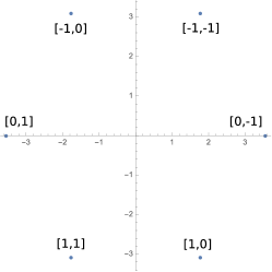
Figure 12: Central charges of BPS particles in the theory at $m=0$, $u=0$, $\Lambda=1$.

Therefore the 3 TBAs at $u=0=m$ read

$$\tilde{\epsilon}_{\gamma_{[1,0]}}(\theta)= |Z|\operatorname{{\rm e}}^{\theta}{-}\frac{1}{2\pi{\rm i}}\left(\int_{\mathbb{R}}\frac{\log(1+\operatorname{{\rm e}}^{-\tilde{\epsilon}_{\gamma_{[0,1]}}(\theta^{\prime})})}{\sinh(\theta-\theta^{\prime}-{\rm i}\frac{2\pi}{3})}{\rm d}\theta^{\prime}+\int_{\mathbb{R}}\frac{\log(1+\operatorname{{\rm e}}^{-\tilde{\epsilon}_{\gamma_{[1,1]}}(\theta^{\prime})})}{\sinh(\theta-\theta^{\prime}-{\rm i}\frac{\pi}{3})}{\rm d}\theta^{\prime}\right),$$ (5.19)

$$\tilde{\epsilon}_{\gamma_{[0,1]}}(\theta)= |Z|\operatorname{{\rm e}}^{\theta}{-}\frac{1}{2\pi{\rm i}}\left(\int_{\mathbb{R}}\frac{\log(1+\operatorname{{\rm e}}^{-\tilde{\epsilon}_{\gamma_{[1,0]}}(\theta^{\prime})})}{\sinh(\theta-\theta^{\prime}-{\rm i}\frac{\pi}{3})}{\rm d}\theta^{\prime}+\int_{\mathbb{R}}\frac{\log(1+\operatorname{{\rm e}}^{-\tilde{\epsilon}_{\gamma_{[1,1]}}(\theta^{\prime})})}{\sinh(\theta-\theta^{\prime}-{\rm i}\frac{2\pi}{3})}{\rm d}\theta^{\prime}\right),$$

$$\tilde{\epsilon}_{\gamma_{[1,1]}}(\theta)= |Z|\operatorname{{\rm e}}^{\theta}{-}\frac{1}{2\pi{\rm i}}\left(\int_{\mathbb{R}}\frac{\log(1+\operatorname{{\rm e}}^{-\tilde{\epsilon}_{\gamma_{[1,0]}}(\theta^{\prime})})}{\sinh(\theta-\theta^{\prime}-{\rm i}\frac{2\pi}{3})}{\rm d}\theta^{\prime}+\int_{\mathbb{R}}\frac{\log(1+\operatorname{{\rm e}}^{-\tilde{\epsilon}_{\gamma_{[0,1]}}(\theta^{\prime})})}{\sinh(\theta-\theta^{\prime}-{\rm i}\frac{\pi}{3})}{\rm d}\theta^{\prime}\right).$$

If we make the ansatz

$$\tilde{\epsilon}_{\gamma_{[1,0]}}(\theta)=\tilde{\epsilon}_{\gamma_{[0,1]}}(\theta)=\tilde{\epsilon}_{\gamma_{[1,1]}}(\theta)\equiv\epsilon(\theta)$$ (5.20)

these 3 equations collapse to a single one,

$$\epsilon(\theta)=|Z|\operatorname{{\rm e}}^{\theta}-\frac{1}{2\pi}\left(\int_{\mathbb{R}}\frac{\log(1+\operatorname{{\rm e}}^{-\epsilon(\theta^{\prime})})}{\cosh(\theta-\theta^{\prime}-{\rm i}\frac{\pi}{6})}{\rm d}\theta^{\prime}+\int_{\mathbb{R}}\frac{\log(1+\operatorname{{\rm e}}^{-\epsilon(\theta^{\prime})})}{\cosh(\theta-\theta^{\prime}+{\rm i}\frac{\pi}{6})}{\rm d}\theta^{\prime}\right).$$ (5.21)

This equation has appeared before in the work of Zamolodchikov; see (post-zamo, , eq. (4.1)) for $b=1/\sqrt{2}$, where it is used to compute Fredholm determinants. We discuss this in more detail in Section 8.2 below.

6 Computation by instanton counting

Another interesting way of computing the quantum periods is by using the NS limit of the instanton counting partition function Braverman:2004cr ; ns ; nrs ; mirmor ; Zenkevich:2011zx . As compared to the other methods presented above, the instanton counting has the advantage of providing analytic expressions in $(E,\hbar,m,\Lambda)$. Nevertheless, the set of spectral problems which we can currently treat within this method is more limited. For example, we do not know how to approach spectral problems associated to non-Lagrangian theories such as the ones in ddt ; Ito:2018eon ; Gaiotto:2014bza .

In this section we use the instanton counting approach to analyze the spectral problem (3.1).

6.1 Definitions

The main quantity that appears in this approach is the Nekrasov-Shatashvili free energy of the $SU(2)$ $N_{f}=1$ theory:

$$F_{\rm NS}(a,\hbar,m,\Lambda)=\sum_{n\geq 1}c_{n}(a,m,\hbar)\Lambda^{3n},$$ (6.1)

where the coefficients $c_{n}$ have a closed form definition in terms of combinatorics of Young diagrams; we refer to (Aminov:2020yma, , Appendix. A) for the definition and a more exhaustive list of references. For example, the first few terms read

$$c_{1} =\frac{2m}{4a^{2}+\hbar^{2}}\,,$$ (6.2)

$$c_{2} =\frac{\left(-48a^{4}+80a^{2}m^{2}-24a^{2}\hbar^{2}-28m^{2}\hbar^{2}-3\hbar^{4}\right)}{16\left(a^{2}+\hbar^{2}\right)\left(4a^{2}+\hbar^{2}\right)^{3}}.$$

It is important to note that (6.1) is exact in $(\hbar,a,m)$ and it is a well-defined convergent sum in the parameter $\Lambda$. Strictly speaking this convergence property has not been proven mathematically (the proofs of felder ; bsu ; ilt do not apply to the $\epsilon_{2}=0$ background); nevertheless, there is considerable numerical evidence for it. In addition one should note that the convergence is for $2{\rm i}a/\hbar\notin{\mathbb{Z}}$, since at these values the NS free energy diverges; see for example Gorsky:2017ndg for a discussion of the structure of these poles. Note also that in four dimensions these poles have a physical meaning, and they should not be confused with the unphysical poles appearing in the five-dimensional uplift of the Nekrasov partition function which were first discussed in Hatsuda:2012dt .

We define $a(E,\hbar,m,\Lambda)$ implicitly via the quantum Matone relation matone ; francisco ,

$$E=\left(a^{2}+{1\over 3}\Lambda\partial_{\Lambda}F_{\rm NS}(a,\hbar,m,\Lambda)\right).$$ (6.3)

This relation defines $a$ only up to an overall sign. We work in the convention where we pick the sign such that ${\rm Re}\left({a\over\hbar}\right)\geq 0$. If ${\rm Re}\left({a\over\hbar}\right)=0$, then we take ${\rm Im}\left({a\over\hbar}\right)>0$. We also define (see for instance Zenkevich:2011zx )

$$a_{D}(a,\hbar,m,\Lambda)={} -4\gamma(2a,\hbar)+\gamma\left(a-m-\frac{{\rm i}\hbar}{2},\hbar\right)+\gamma\left(a+m-\frac{{\rm i}\hbar}{2},\hbar\right)+\partial_{a}F_{\rm NS}(a,\hbar,m,\Lambda)$$ (6.4)

$$+{\rm i}\pi a-{\rm i}\pi m+\frac{1}{2}{\rm i}\hbar\log\left({\mathrm{e}}^{\frac{2\pi(m-a)}{\hbar}}+1\right)-\frac{1}{2}{\rm i}\hbar\log\left({\mathrm{e}}^{-\frac{2\pi(a+m)}{\hbar}}+1\right)$$

$$+6a\log(\Lambda)+\frac{1}{2}{\rm i}\hbar\log\left(a-m-\frac{{\rm i}\hbar}{2}\right)+\frac{1}{2}{\rm i}\hbar\log\left(a+m-\frac{{\rm i}\hbar}{2}\right),$$

where

$$\gamma(a,\hbar)=\left(-\frac{1}{2}a\log\left(\frac{1}{\hbar^{2}}\right)-\frac{\pi\hbar}{4}\right)-\frac{1}{2}{\rm i}\hbar\left(\log\Gamma\left(\frac{{\rm i}a}{\hbar}+1\right)-\log\Gamma\left(1-\frac{{\rm i}a}{\hbar}\right)\right).$$ (6.5)

Note that

$$a_{D}(a,\hbar,m,\Lambda)=a_{D}(-a,-\hbar,m,\Lambda)+{\rm i}\hbar\left(\log\left(\operatorname{{\rm e}}^{\frac{2\pi a}{\hbar}}+\operatorname{{\rm e}}^{\frac{2\pi m}{\hbar}}\right)-\log\left(\operatorname{{\rm e}}^{\frac{2\pi(a+m)}{\hbar}}+1\right)\right).$$ (6.6)

For later purposes it is useful to define

$$a_{m}(a,\hbar,{m},\Lambda)={} \gamma\left(a+{m}-\frac{{\rm i}\hbar}{2},\hbar\right)-\gamma\left(a-{m}-\frac{{\rm i}\hbar}{2},\hbar\right)+\partial_{m}F_{\rm NS}(a,\hbar,{m},\Lambda)$$ (6.7)

$$-\frac{1}{2}{\rm i}\hbar\log\left(a-{m}-\frac{{\rm i}\hbar}{2}\right)+\frac{1}{2}{\rm i}\hbar\log\left(a+{m}-\frac{{\rm i}\hbar}{2}\right)-\frac{1}{2}{\rm i}\hbar\log\left({\mathrm{e}}^{\frac{2\pi({m}-a)}{\hbar}}+1\right)$$

$$-\frac{1}{2}{\rm i}\hbar\log\left({\mathrm{e}}^{-\frac{2\pi(a+{m})}{\hbar}}+1\right)+2{\rm i}\hbar\log\left(1-{\mathrm{e}}^{-\frac{4\pi a}{\hbar}}\right),$$

and the normalized quantities

$${\tt a}(E,\hbar,m,\Lambda):= -{4\pi a\over\hbar}(E,\hbar,m,\Lambda),$$ (6.8)

$${\tt a}_{D}(E,\hbar,m,\Lambda):= -{{\rm i}\over\hbar}a_{D}(a,\hbar,m,\Lambda)\Big{|}_{a=a(E,\hbar,m,\Lambda)},$$

$${\tt a}_{m}(E,\hbar,m,\Lambda):= {{\rm i}\over\hbar}a_{m}(a,\hbar,m,\Lambda)\Big{|}_{a=a(E,\hbar,m,\Lambda)}.$$

Then we have

$${\tt a}(E,\hbar,m,\Lambda)\quad\xrightarrow{\hbar\to 0}\quad\sum_{n\geq 0}\hbar^{2n-1}{\tt a}^{(n)}(E,m,\Lambda),$$ (6.9)

$${\tt a}_{D}(E,\hbar,m,\Lambda)\quad\xrightarrow{\hbar\to 0}\quad\sum_{n\geq 0}\hbar^{2n-1}{\tt a}_{D}^{(n)}(E,m,\Lambda).$$ (6.10)

Let us note that, even though ${\tt a}$ and ${\tt a}_{D}$ are well defined both in the strong and weak coupling region, the series expansion coefficients ${\tt a}^{(n)}$ and ${\tt a}_{D}^{(n)}$ converge only in the weak coupling region.

Another important observation, due to mirmor ; Zenkevich:2011zx , is that the series expansion coefficients ${\tt a}^{(n)}$ and ${\tt a}_{D}^{(n)}$ coincide with the WKB coefficients $\Pi_{\gamma}^{(n)}$ of the quantum periods in equation (3.26) if the cycle $\gamma$ is suitably chosen. Hence instanton counting provides an exact, analytic resummation of the WKB series.

6.2 Quantum periods

Now we want to describe the relation between ${\tt a}$, ${\tt a}_{D}$ and the quantum periods $\Pi_{\gamma}$ as we have defined them.

As we reviewed in Section 2, the $\Pi_{\gamma}$ are piecewise analytic; to make an honest analytic function from them we have to fix a basepoint $(\vartheta,u_{0},m_{0},\Lambda_{0})$. Thus, to compare them to ${\tt a}$, ${\tt a}_{D}$ we need to pick such a basepoint. Experimentally, we find that the right basepoint to choose (within the weak coupling region) is one leading to a Schrödinger equation (3.1) with a real convex confining potential along some $x$-direction. This condition is fulfilled for

$$2\arg(\Lambda)-{\rm Im}(x)-2\arg(\hbar)={} 2\pi\ell_{1}\,,$$ (6.11)

$$\arg(m)+\arg(\Lambda)+{\rm Im}(x)-2\arg(\hbar)={} 2\pi\ell_{2}\,,$$

$$2\arg(\Lambda)+2{\rm Im}(x)-2\arg(\hbar)+\pi={} 2\pi\ell_{3}\,,$$

$$\arg(u)-2\arg(\hbar)={} 2\pi\ell_{4}\,,$$

where $\ell_{i}\in{\mathbb{Z}}$. This leaves us with a variety of possibilities, but we expect the final result to be independent of this choice. Hence we can take (hopefully without loss of generality)

$$m_{0}^{\rm inst}={{\rm i}\over 10},\quad u_{0}^{\rm inst}=2,\quad\Lambda_{0}^{\rm inst}=\operatorname{{\rm e}}^{-{\rm i}\pi/6}\,.$$ (6.12)

Moreover, inspired by nrs ; Hollands:2019wbr ; Grassi:2019coc ; Hollands:2013qza ; Hollands:2017ahy , we expect that instanton counting corresponds to Fenchel-Nielsen coordinates, namely to spectral coordinates at

$$\vartheta^{\rm inst}_{0}={\arg}(-Z_{\gamma_{a}}(u_{0}^{\rm inst},m_{0}^{\rm inst},\Lambda_{0}^{\rm inst}))=0$$ (6.13)

where $Z_{\gamma_{a}}$ is the central charge of the vectormultiplet in the BPS spectrum at weak coupling. Hence we propose the identification

$$\Pi_{\gamma_{[0,2,0]}}^{{\rm inst},\vartheta_{0}^{\rm inst},m_{0}^{\rm inst},u_{0}^{\rm inst},\Lambda_{0}^{\rm inst}}(E,\hbar,m,\Lambda)={\tt a}(E,\hbar,m,\Lambda),$$ (6.14)

as well as

$$\Pi_{\gamma_{[1,0,0]}}^{{\rm inst},\vartheta_{0}^{\rm inst},m_{0}^{\rm inst},u_{0}^{\rm inst},\Lambda_{0}^{\rm inst}}(E,\hbar,m,\Lambda)={\tt a}_{D}(E,\hbar,m,\Lambda),$$ (6.15)

where the charges $\gamma_{[1,0,0]}$ and $\gamma_{[0,2,0]}$ are taken relative to the basis in Figure 11.

We also have as usual the exact formula

$$\Pi^{{\rm inst},\vartheta_{0}^{\rm inst},m_{0}^{\rm inst},u_{0}^{\rm inst},\Lambda_{0}^{\rm inst}}_{\gamma_{[0,0,1]}}=-2\pi m/\hbar.$$ (6.16)

We will denote by ${C}^{\rm inst}$ the locus specified by (6.12), (6.13).

7 Comparisons

In the last few sections we have described four different ways of understanding, and numerically computing, the quantum periods in the $SU(2)$ $N_{f}=1$ theory. Our expectation is that all four methods are approximating the same functions $\Pi_{\gamma}$, so that our four numerical computations should agree, up to the inherent numerical error in the various methods. The results of various such comparisons are reported in Table 1. In this section we discuss in more detail some examples, and some subtleties that arise in making the comparison.

7.1 Comparisons in the weak coupling region

7.1.1 Instanton counting versus small section method

We first compare instanton counting with the SS method of Section 4, i.e. we compare $\Pi^{\rm inst}$ with $\Pi^{\rm SS}$.

We recall that when we use the SS method we need to specify two set of parameters:

• One set of parameters

  $$\vartheta,u_{0},m_{0},\Lambda_{0}$$ (7.1)

  specifying the spectral network $\mathcal{W}$ that we use in the computation.

• One set of parameters

  $$\hbar,u,m,\Lambda$$ (7.2)

  specifying the values at which we evaluate the spectral coordinates $\mathcal{X}^{\rm SS}_{\gamma}$.

In Section 4 we always used $(u_{0},m_{0},\Lambda_{0})=(u,m,\Lambda)$ and hence we only needed to specify the parameter $\vartheta$. This is the reason why we used the notation $\mathcal{W}^{\vartheta}$ instead of $\mathcal{W}^{\vartheta,u_{0},m_{0},\Lambda_{0}}$. For comparing with instanton counting, it is more convenient to choose $(\vartheta,u_{0},m_{0},\Lambda_{0})$ lying in the instanton locus $C^{\rm inst}$. The spectral network which appears then is the one we used in Section 4.4, and the concrete Wronskian formulas we use are the ones in that section as well.

As an example, we take

$$E=3+{{\rm i}/5},\quad m={{\rm i}\over 2}+{3\over 10},\quad\Lambda={1\over 5}+{\frac{{\rm i}}{10}},\quad\hbar=1+{{\rm i}\over 2}.$$ (7.3)

We evaluate $\Pi_{\gamma_{[1,0,0]}}$ by using instanton counting and compare with the result from the SS method (concretely, (4.32)). We find good agreement:

$$\Pi_{\gamma_{[1,0,0]}}^{\rm inst,\vartheta=0,m_{0}^{\rm inst},u_{0}^{\rm inst},\Lambda_{0}^{\rm inst}}={\tt a}_{D}= ~{}14.5926368914\ldots+11.9576187144~{}{\rm i}\ldots$$ (7.4)

$$\Pi_{\gamma_{[1,0,0]}}^{\rm SS,\vartheta=0,m_{0}^{\rm inst},u_{0}^{\rm inst},\Lambda_{0}^{\rm inst}}= ~{}14.5926368914\ldots+11.9576187144~{}{\rm i}\ldots$$

More comparisons are shown in Table 1. In that table, though, we report the canonical $\Pi_{\gamma}$, or said otherwise, we take $(\vartheta,u_{0},m_{0},\Lambda_{0})=(\arg\hbar,u,m,\Lambda)$. Thus, in particular, the quantities $\Pi_{\gamma}^{\rm inst}$ appearing in that table are in general not equal to ${\tt a}$, ${\tt a}_{D}$; rather they are related by the appropriate KS transformations to move to the correct chamber. We discuss this procedure in more detail in the next section.

7.1.2 Instanton counting versus Borel summation

Let us now look at Borel summation. As we have recalled in Section 2, Borel summation always produces the canonical $\Pi_{\gamma}$, i.e. the ones at $(\vartheta,u_{0},m_{0},\Lambda_{0})=(\arg\hbar,u,m,\Lambda)$. Therefore, if we pick $(\arg\hbar,u,m,\Lambda)\in C^{\rm inst}$, then instanton counting and (median) Borel summation should agree. This is the analogue of what was done in Grassi:2019coc . However, for generic values of the parameters we need to implement an appropriate KS transformation.

As an example we can take

$$E=4,\quad m=0,\quad\Lambda={1\over 5},\quad\hbar=1+{\frac{{\rm i}}{10}}\,.$$ (7.5)

We consider the period $\Pi_{\gamma}$ for $\gamma=\gamma_{a_{D}}=\gamma_{[1,0,0]}$. The point (7.5) is not on any wall; in particular, the WKB series $\Pi^{\mathrm{WKB}}_{\gamma}$ at this point is Borel summable, without requiring median summation, and gives $\Pi_{\gamma}$ at the point (7.5). However, since the point (7.5) $\notin C^{\rm inst}$, to compare this Borel sum with instanton counting we have to work out the transformation between $\Pi^{\eqref{chBorel}}$ and $\Pi^{C^{\rm inst}}$. For that purpose we choose a particular path connecting these two points, and apply the transformations (2.1)-(2.3) for all the BPS states which we encounter along this path.

As a first step, we vary $\hbar$ along a path from (7.5) to an intermediate chamber

$$E=4,\quad m=0,\quad\Lambda={1\over 5},\quad\hbar=0\,.$$ (7.6)

On this path we encounter the BPS states whose central charges satisfy

$$0\leq-Z_{\gamma_{\rm BPS}}\leq\arg(1+\frac{{\rm i}}{10});$$ (7.7)

these central charges are

$$-Z_{\gamma_{[0,2,0]}},-Z_{\gamma_{[0,1,1]}},-Z_{\gamma_{[0,1,-1]}},\quad$$ (7.8)

as well as

$$-Z_{\gamma_{n}}={} -Z_{-\gamma_{a_{D}}}-nZ_{\gamma_{a}},\quad n\geq 11,$$ (7.9)

$$-Z_{\overline{\gamma_{m}}}={} -\overline{Z_{\gamma_{a_{D}}}}-mZ_{\gamma_{a}},\quad m\geq 11.$$

Some of them can be seen explicitly in 7(d). Note that there will be infinite BPS states in 7(d) if we take infinite terms $\Pi^{n}$ in the series expansion. We get

$$\Pi_{\gamma_{a_{D}}}^{\eqref{chBorelp}} =\Pi_{\gamma_{a_{D}}}^{\eqref{chBorel}}-\frac{1}{2}\log(1+\mathcal{X}^{\vartheta=0}_{\gamma_{[0,1,1]}})-\frac{1}{2}\log(1+\mathcal{X}^{\vartheta=0}_{\gamma_{[0,1,-1]}})-\frac{1}{2}\log(1-\mathcal{X}^{\vartheta=0}_{\gamma_{[0,2,0]}})^{-4}$$ (7.10)

$$-\sum_{n\geq 11}2n\log\left(\left(1+\mathcal{X}^{\vartheta={\arg}(-Z_{\gamma_{n}})}_{\gamma_{n}}\right)\left(1+\mathcal{X}^{\vartheta={\arg}(-{Z_{\overline{\gamma_{n}}}})}_{\overline{\gamma}_{n}}\right)\right).$$

At the practical level, we can neglect the last sum since the largest contribution in this infinite series can be approximated by

$$\log(\sqrt{(1+\exp\left[-Z_{\overline{\gamma_{11}}}(1+{\rm i}/10)^{-1}\right])})\approx 10^{-120}{\rm i}$$ (7.11)

which is much smaller than the accuracy we can reach with Borel summation of 80 even terms.

As a second step on our path we go from (7.6) to $C^{\rm inst}$, by turning on a small $m\in{\mathrm{i}}\mathbb{R}_{+}$. In this procedure only $-Z_{\gamma_{[0,1,-1]}}$ and $-Z_{\gamma_{[0,1,1]}}$ contribute to (2.1)-(2.3). We sketch this in Figure 13. We have

$$\Pi^{\rm C^{\rm inst}}_{\gamma_{a_{D}}}=\Pi_{\gamma_{a_{D}}}^{\rm\eqref{chBorelp}}-\frac{1}{2}\log(1+\mathcal{X}^{\rm\vartheta=0}_{\gamma_{[0,1,1]}})+\frac{1}{2}\log(1+\mathcal{X}^{\rm\vartheta=0}_{\gamma_{[0,1,-1]}}).$$ (7.12)

Now combining (7.10) and (7.12), we have

$$\Pi^{C^{\rm inst}}_{\gamma_{a_{D}}}\approx\Pi_{\gamma_{a_{D}}}^{\eqref{chBorel}}-\log(1+\mathcal{X}^{\vartheta=0}_{\gamma_{[0,1,1]}})-\frac{1}{2}\log(1-\mathcal{X}^{\vartheta=0}_{\gamma_{[0,2,0]}})^{-4}\,,$$ (7.13)

where $\approx$ means that we are neglecting second line of (7.10).

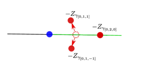
Figure 13: Zoom in around the real axis. The dashed circle represents the singularities from the 2 hypermultiplets with $-Z_{\gamma_{[0,1,1]}}=-Z_{\gamma_{[0,1,-1]}}$ in massless case. Changing from (7.6) to ${C^{\rm inst}}$ corresponds to split the dashed circle into two red dots representing the singularities at $-Z_{\gamma_{[0,1,-1]}}$ and the $-Z_{\gamma_{[0,1,1]}}$. The green ray represents $\vartheta=0$.

The final contribution from each KS transformation are listed in Table 3.

$\Pi_{\gamma_{a_{D}}}^{\rm PB}(E,\hbar,m,\Lambda)$	$\underline{8.87942}7505929998+\underline{25.70889}962041928{\rm i}$
$\Pi_{\gamma_{a_{D}}}^{\rm PB}(E,\hbar,m,\Lambda)$
$-\log(1+\mathcal{X}^{\rm PB,\vartheta=0}_{\gamma_{[0,1,1]}})$	$\underline{8.8794262388}60653+\underline{25.708895879}81361{\rm i}$
$\Pi_{\gamma_{a_{D}}}^{\rm PB}(E,\hbar,m,\Lambda)$
$-\log(1+\mathcal{X}^{\rm PB,\vartheta=0}_{\gamma_{[0,1,1]}})$
$+2\log({1-\mathcal{X}^{\rm PB,\vartheta=0}_{\gamma_{[0,2,0]}}})$	8.879426238885426 + 25.70889587979465 i
${\tt a}_{D}(E,\hbar,m,\Lambda)$	8.879426238885426 + 25.70889587979465 i

Table 3: Transformation to compare Padé-Borel summation $\Pi_{\gamma_{a_{D}}}^{\rm PB}$ with ${\tt a}_{D}$ according to (7.13). The parameters used are $E=4,m=0,\Lambda={1\over 5},\hbar=1+{\frac{{\rm i}}{10}}$.

Another example we use in this paper is

$$E=4,\quad m={\rm i}/10,\quad\Lambda=\operatorname{{\rm e}}^{-\pi{\rm i}/6},\quad\hbar=1/2\,.$$ (7.14)

The results are shown in Table 4.

Here we mention some technical problems encountered in the Padé-Borel method and show how we can nicely overcome such obstacles by taking advantage of the KS transformation and the knowledge about the underlying gauge theory.

Let us consider for example 7(f) and 7(d). The red dot on the positive real axis represents the two hypermultiplets with central charges $Z_{\gamma_{[0,1,-1]}}=Z_{\gamma_{[0,1,1]}}$, indeed in this example $Z_{\gamma_{[0,0,1]}}=-2\pi m=0$. However, there should also be a singularity at the central charge of the vectormultiplet $\gamma_{[0,2,0]}$. Nevertheless, we do not see it explicitly in the Borel plane because the singularity at $Z_{\gamma_{[0,1,-1]}}=Z_{\gamma_{[0,1,1]}}$ spans a full series of poles which mix with the poles corresponding to $Z_{\gamma_{[0,2,0]}}$. As a consequece the discontinuities at $Z_{\gamma_{[0,1,1]}}=Z_{\gamma_{[0,1,-1]}}$ and $Z_{\gamma_{[0,2,0]}}$ will also mix. However in our computations, in particular when implementing the KS transform as in Table 3, we need to take this singularity into account even if we do not see it explicitly in the Borel plane. It could be that by combining Padé-Borel with some more advanced techniques we might be able to see these three singularities separately. A more general phenomenon also appears when $m\neq 0$. For example, when we study the Padé-Borel transform for $\gamma_{[1,0,0]}$ at (7.14). Such transform has two series of poles close to the real axis, see 7(g), which correspond to the 2 hypermultiplets $\gamma_{[0,1,1]}$ and $\gamma_{[0,1,-1]}$. These series of poles point towards the real axis where they collide and then carry on as a unique series close to the real axis. Because of their existence, we can not see the series of poles representing the vector multiplet $\gamma_{[0,2,0]}$. In addition in 7(i), when the series of poles for finite number of terms from the two hypermultiplets seems rotated to slightly different direction from real axis, the interference still makes the vectormultiplet hard to be seen. The mixing of these poles makes it impossible to find a path of integration for the lateral Padé-Borel summation around $\arg(\hbar)=0$ which is not affected by the poles of 2 hypermultiplets and take half effect of the vectormultiplet. We overcome this technical obstacle by taking advantage of the KS transformation. We take the direction of integration to be ${\mathbb{R}}_{+}\operatorname{{\rm e}}^{{\rm i}/10}$ so that we are in the chamber $\vartheta=1/10$. Padé-Borel summation work in this chamber and then we use KS transformation to transform it back to chamber (7.14). The leading contribution to such transformation comes from the hypermultiplet with charge $\gamma_{[0,1,1]}$. The results are shown in Table 4.

$\Pi^{\rm PB,\vartheta=\frac{1}{10}}_{\gamma_{a_{D}}}(E,\hbar,m,\Lambda)$	$3.9*10^{-12}+14.0834766258633{\rm i}$
$\Pi^{\rm PB,\vartheta=\frac{1}{10}}_{\gamma_{a_{D}}}(E,\hbar,m,\Lambda)$
$-\log(1+\mathcal{X}^{\rm PB,\vartheta=\frac{1}{10}}_{\gamma_{[0,1,1]}})$	$14.0834766258755{\rm i}$
${\tt a}_{D}(E,\hbar,m,\Lambda^{\prime})$	$14.0834766258755{\rm i}$

Table 4: Transformation to compare Padé-Borel summation $\Pi_{\gamma_{a_{D}}}^{\rm PB}$ with ${\tt a}_{D}$. The parameters used for $E,\hbar,m,\Lambda$ are those in (7.14).

We conclude this part with a comment on the poles of the four dimensional NS free energy. As anticipated earlier the NS free energy (and in particular the ${\tt a}_{D}=\Pi_{\gamma_{[1,0,0]}}^{C^{\rm inst}}$ period) has poles if $2a{\rm i}/\hbar\in{\mathbb{Z}}$, i.e. if $(E,\Lambda,m,\hbar)$ are such that

$$\Pi_{\gamma_{[0,2,0]}}^{C^{\rm inst}}(E,\Lambda,m,\hbar)=2\pi{\rm i}{\mathbb{Z}}.$$ (7.15)

On the other hand we know that at such values of $(E,\Lambda,m,\hbar)$ Borel summation gives a well defined number for $\Pi_{\gamma_{[1,0,0]}}(E,\Lambda,m,\hbar)$. The reason for such different behaviour is due to the fact that when (7.15) holds, the KS transform for the vector multiplet is singular. Hence the transformation between instanton and Borel chamber is singular.

7.2 Comparison in strong coupling region

In the strong coupling region the relation between instanton counting and small section method is much more complicated. The reason is that the topology of the spectral network at strong coupling is very different from the one making contact with instanton counting, namely (6.12). Indeed, if we follow a path from the instanton locus to strong coupling which avoids singularities in the Coulomb branch, we will have to cross an infinite number of walls, and thus encounter an infinite tower of transformations (2.1)-(2.3). To avoid such a complicated calculation, we can use the following procedure.

At $\vartheta_{0}^{\rm inst},u_{0}^{\rm inst},{m}_{0}^{\rm inst},\Lambda_{0}^{\rm inst}$, we choose a basis in which the monodromy matrix and its eigenvectors are

$$M=\begin{pmatrix}\frac{1}{\mu}&0\\ 0&\mu\end{pmatrix},\quad\psi_{4}=\left(\begin{matrix}1\\ 0\\ \end{matrix}\right),\quad\psi_{5}=\left(\begin{matrix}0\\ 1\\ \end{matrix}\right)$$ (7.16)

We start from the weak coupling region at $E_{0}^{\rm inst}=4,~{}\Lambda^{\rm inst}_{0}=\exp(-{\rm i}\pi/6),~{}m_{0}^{\rm inst}=\frac{{\rm i}}{10}$, with $\mathcal{W}^{\vartheta=\vartheta_{0}^{\rm inst}=0}$. By matching the small section result (4.31), (4.32)

$$\mathcal{X}^{\rm SS,\vartheta=\vartheta_{0}^{\rm inst},u=u_{0}^{\rm inst},{m}={m}_{0}^{\rm inst},\Lambda=\Lambda_{0}^{\rm inst}}(\hbar,u,m,\Lambda)$$

with the instanton counting result (6.14), (6.15)

$$\mathcal{X}^{\rm inst,\vartheta_{0}^{\rm inst},u_{0}^{\rm inst},{m}_{0}^{\rm inst},\Lambda_{0}^{\rm inst}}(\hbar,u,m,\Lambda)$$

we deduce that

$$\psi_{1}= \left(\begin{matrix}\psi_{1,1}\\ 1\\ \end{matrix}\right),$$ (7.17)

$$\psi_{2}= \left(\begin{matrix}-\psi_{1,1}\operatorname{{\rm e}}^{{\tt a}_{\rm D}}\\ 1\\ \end{matrix}\right),$$

$$\psi_{3}= \left(\begin{matrix}\psi_{1,1}\left(-\operatorname{{\rm e}}^{{\tt a}_{\rm D}+\frac{{\tt a}}{2}}\right)\cosh\left(\frac{{\tt a}}{4}-\frac{\pi m}{h}\right)\text{sech}\left(\frac{{\tt a}}{4}+\frac{\pi m}{h}\right)\\ 1\\ \end{matrix}\right),$$

for some $\psi_{1,1}$ which we do not need to determine for our purpose. Even though these expressions have been derived at weak coupling, by analytic continuation they hold at strong coupling as well. Therefore the spectral coordinates at strong coupling, given in (4.10), (4.11), (4.12), become

$$\mathcal{X}_{\gamma_{[1,0,0]}}^{\rm inst,\vartheta=0}(\hbar,u,m,\Lambda)=\frac{\operatorname{{\rm e}}^{{\tt a}_{\rm D}}\left(\operatorname{{\rm e}}^{{\tt a}}-1\right)\sqrt{\frac{\operatorname{{\rm e}}^{-{\tt a}_{\rm D}}\left(\left(\operatorname{{\rm e}}^{{\tt a}_{\rm D}}+1\right)\operatorname{{\rm e}}^{\frac{{\tt a}}{2}-\frac{2\pi m}{h}}+\operatorname{{\rm e}}^{{\tt a}_{\rm D}}+\operatorname{{\rm e}}^{{\tt a}}\right)}{e^{{\tt a}_{\rm D}+{\tt a}}+1}}}{\left(\operatorname{{\rm e}}^{{\tt a}_{\rm D}}+1\right)\operatorname{{\rm e}}^{\frac{{\tt a}}{2}+\frac{2\pi m}{h}}+\operatorname{{\rm e}}^{{\tt a}_{\rm D}+{\tt a}}+1},$$ (7.18)

$$\mathcal{X}_{\gamma_{[0,1,1]}}^{\rm inst,\vartheta=0}(\hbar,u,m,\Lambda)=\frac{\operatorname{{\rm e}}^{-{\tt a}_{\rm D}+\frac{{\tt a}}{2}-\frac{2\pi m}{h}}\left(\left(\operatorname{{\rm e}}^{{\tt a}_{\rm D}}+1\right)^{2}\operatorname{{\rm e}}^{\frac{{\tt a}}{2}+\frac{2\pi m}{h}}+\operatorname{{\rm e}}^{{\tt a}_{\rm D}}\left(\operatorname{{\rm e}}^{{\tt a}_{\rm D}+{\tt a}}+\operatorname{{\rm e}}^{{\tt a}}+1\right)+1\right)}{\left(\operatorname{{\rm e}}^{{\tt a}}-1\right)^{2}}\,,\\$$ (7.19)

$$\mathcal{X}_{\gamma_{[-1,-1,1]}}^{\rm inst,\vartheta=0}(\hbar,u,m,\Lambda)=-\frac{\operatorname{{\rm e}}^{{\tt a}_{\rm D}}\left(\operatorname{{\rm e}}^{{\tt a}}-1\right)\sqrt{\frac{\left(\operatorname{{\rm e}}^{{\tt a}_{\rm D}+{\tt a}}+1\right)}{\left(\operatorname{{\rm e}}^{{\tt a}_{\rm D}}+1\right)\operatorname{{\rm e}}^{{\tt a}_{\rm D}+\frac{3{\tt a}}{2}+\frac{2\pi m}{h}}+\left(\operatorname{{\rm e}}^{{\tt a}_{\rm D}}+\operatorname{{\rm e}}^{{\tt a}}\right)\operatorname{{\rm e}}^{{\tt a}_{\rm D}+{\tt a}+\frac{4\pi m}{h}}}}}{\left(\operatorname{{\rm e}}^{{\tt a}_{\rm D}}+1\right)}\,,$$ (7.20)

where on the r.h.s. we used the shortcut notation

$${\tt a}={\tt a}(\hbar,u,m,\Lambda),\quad{\tt a}_{D}={\tt a}_{D}(\hbar,u,m,\Lambda)\,.$$ (7.21)

We also show expressions for $m=0$:

$$\mathcal{X}_{\gamma_{[1,0,0]}}^{\rm inst,\vartheta=0}(\hbar,u,m=0,\Lambda)=\frac{\sinh\left(\frac{{\tt a}}{4}\right)\sqrt{\left(\cosh\left(\frac{{\tt a}_{\rm D}-{\tt a}}{2}\right)+\cosh\left(\frac{{\tt a}_{\rm D}}{2}\right)\right)\text{sech}\left(\frac{{\tt a}_{\rm D}+{\tt a}}{2}\right)}}{\sinh\left(\frac{1}{4}({\tt a}+2{\tt a}_{\rm D})\right)},$$ (7.22)

$$\mathcal{X}_{\gamma_{[0,1,1]}}^{\rm inst,\vartheta=0}(\hbar,u,m=0,\Lambda)=\frac{1}{2}\cosh\left(\frac{{\tt a}_{\rm D}}{2}\right)\text{csch}^{2}\left(\frac{{\tt a}}{4}\right)\text{sech}\left(\frac{{\tt a}}{4}\right)\cosh\left(\frac{1}{4}(2{\tt a}_{\rm D}+{\tt a})\right),$$ (7.23)

$$\mathcal{X}_{\gamma_{[-1,-1,1]}}^{\rm inst,\vartheta=0}(\hbar,u,m=0,\Lambda)=-\frac{\sinh\left(\frac{{\tt a}}{4}\right)\sqrt{2\cosh\left(\frac{{\tt a}}{4}\right)\cosh\left(\frac{{\tt a}+{\tt a}_{\rm D}}{2}\right)\text{sech}\left(\frac{1}{4}({\tt a}-2{\tt a}_{\rm D})\right)}}{\text{cosh}\left(\frac{{\tt a}_{\rm D}}{2}\right)}.$$ (7.24)

The equations above are the transformations between Fock-Goncharov coordinates and Fenchel-Nielsen coordinates (instanton counting).

The results are in Table 1, where the spectral coordinates reported are at $\vartheta=\arg(\hbar)$. For our examples with $u=0$, $m\in\{0,-1/10\}$, $\Lambda\in\{1,{1\over 5}\}$ and $\arg(\hbar)=\arg(1+{\frac{{\rm i}}{10}})$, we have

$$\Pi_{\gamma[-1,-1,1]}={} \Pi_{\gamma[-1,-1,1]}^{\vartheta=0}-{1\over 2}\log\left(1+\mathcal{X}^{\vartheta=0}_{[0,1,1]}\right),$$ (7.25)

$$\Pi_{\gamma[1,0,0]}={} \Pi_{\gamma[1,0,0]}^{\vartheta=0}+{1\over 2}\log\left(1+\mathcal{X}^{\vartheta=0}_{[0,1,1]}\right),$$

$$\Pi_{\gamma[0,1,1]}={} \Pi_{\gamma[0,1,1]}^{\vartheta=0}.$$

Notice that the r.h.s. of (7.18)-(7.20) provides an analytic solution to the GMN TBA at strong coupling (after we implement (7.25)).

We conclude this section with a brief comment on Painlevé equations. It was suggested in Coman:2020qgf , based on ilt , that the transformations between Fock-Goncharov and Fenchel-Nielsen coordinates are useful in the study of the connection problems in Painlevé equations. From this point of view the transformations (7.22)-(7.24) could play and interesting role in the study of the connection problem for Painlevé $\rm III_{2}$.

8 Fredholm determinant

8.1 From Topological String

A convenient way to encode the spectral properties of a given trace class operator $\rm O^{-1}$ is by using the Fredholm determinant

$$\det\left(1-{E\over{\rm O}}\right).$$ (8.1)

Such object is also interesting from a physical point of view since it is an entire function in $E$ which is usually identified with the Coulomb branch parameter. The computation of these determinant is a challenging question. In some situations we can use (numerical) TBA techniques or WKB analysis post-zamo ; voros-zeta ; voros ; voros-zq ; voros-quartic . However if the operator $\rm O$ has an interpretation in terms of quantum mirror curve to toric CY manifolds, then its Fredholm determinant can be computed explicitly and exactly ghm ; cgm ; cgm8 . Such construction was originally formulated only in some particular slice of the moduli space where the operators have a positive discrete spectrum with bound states. This was later generalised in cgum ; gm17 ; gm3 to include operators with complex eigenvalues and in particular resonance states. The operator we are studying in this paper (3.1) does not correspond to a quantum mirror curve to toric manifolds. Nevertheless it can be obtained from such construction after implementing the geometric engineering limit kkv ; selfdual , similar to what was done in Grassi:2019coc for the (modified) Mathieu example.

We are interested in the toric CY geometry that engineers the $SU(2)$ 4d $N_{f}=1$ theory, namely local ${\mathbb{F}}_{2}$ blown up at 1 point as in kkv . We denote this geometry as local ${{\cal B}}{\mathbb{F}}_{2}$. The the quantum mirror curve for this CY is

$$a_{1}+a_{2}\operatorname{{\rm e}}^{\hat{y}}+\operatorname{{\rm e}}^{\hat{x}}+a_{4}\operatorname{{\rm e}}^{-\hat{x}-\hat{y}}+a_{5}\operatorname{{\rm e}}^{-2\hat{x}-\hat{y}}+\operatorname{{\rm e}}^{-\hat{x}}=0,\quad[\hat{x},\hat{p}]={\rm i}\hbar$$ (8.2)

where $a_{i}$ are expressed by using the Batyrev coordinates $z_{i}$ as

$$z_{1} ={a_{5}\over a_{1}a_{4}},$$ (8.3)

$$z_{2} ={a_{4}\over a_{1}a_{5}},$$

$$z_{3} ={a_{2}a_{5}}.$$

Topological string partition function on toric CY manifolds corresponds to Nekrasov function for five dimensional gauge theory on $S_{1}\times{{\mathbb{R}}}^{4}_{\epsilon_{1},\epsilon_{2}}$, see for instance nek5 . Hence it is useful to use the parametrisation

$$z_{1} ={\operatorname{{\rm e}}^{mR}\over H},$$ (8.4)

$$z_{2} ={\operatorname{{\rm e}}^{-mR}\over H}$$

$$z_{3} =\Lambda^{3}R^{3},$$

where $\Lambda$ is the instanton counting parameter of the five dimensional gauge theory, $H$ is a coulomb branch parameter, $m$ plays the role of a mass parameter and $R$ is the radius of $S_{1}$. This parametrisation will be useful later. The operator we study in the setup of ghm ; cgm is

$${\rm O_{{{\cal B}}{\mathbb{F}}_{2}}}=a_{2}\operatorname{{\rm e}}^{\hat{p}}+\operatorname{{\rm e}}^{\hat{x}}+a_{4}\operatorname{{\rm e}}^{-\hat{x}-\hat{p}}+a_{5}\operatorname{{\rm e}}^{-2\hat{x}-\hat{p}}+\operatorname{{\rm e}}^{-\hat{x}},\quad[\hat{x},\hat{p}]={\rm i}\hbar.$$ (8.5)

We think of $\rm O_{{{\cal B}}{\mathbb{F}}_{2}}$ as an operator on functions in $L^{2}({\mathbb{R}})$ which admit an analytic continuation on the strip $\pm{\rm i}\hbar$. Then, according to ghm ; cgm , we have

$$\det(1-\operatorname{{\rm e}}^{\mu}\rho)=\sum_{n\in{\mathbb{Z}}}\operatorname{{\rm e}}^{{\rm J}(\mu+2\pi{\rm i}n+{\rm i}\pi,\mu_{1}+{\rm i}\pi,\mu_{2},\mu_{3},\hbar)},$$ (8.6)

where $\rho={\rm O}_{{{\cal B}}{\mathbb{F}}_{2}}^{-1}$ and we use the following dictionary

$$a_{1}=\operatorname{{\rm e}}^{\mu+{\rm i}\pi},\quad a_{4}=\operatorname{{\rm e}}^{\mu_{1}+{\rm i}\pi},\quad a_{5}=\operatorname{{\rm e}}^{\mu_{2}},\quad a_{2}=\operatorname{{\rm e}}^{\mu_{3}}.$$ (8.7)

The quantity ${\rm J}$ in (8.6) is the topological string grand potential associated to the local ${{\cal B}}{\mathbb{F}}_{2}$ geometry. A self-contained definition is given for instance in (mmrev, , eq. (93)) or (cgm, , Sec. 3.1).

We now implement the geometric engineering limit on (8.6). Let us first look at the operator $\rm O_{{{\cal B}}{\mathbb{F}}_{2}}$. In this limit we rescale

$$\hat{x}\to R\hat{x},\quad\hbar\to R\hbar$$ (8.8)

and take $R\to 0$. After removing the overall $R^{2}$ factor, we are left with the following operator

$$\left(\Lambda^{3}\operatorname{{\rm e}}^{\hat{p}}+(\hat{x}+m+{{\rm i}\hbar\over 2})\operatorname{{\rm e}}^{-\hat{p}}\right)+\hat{x}^{2},\quad[\hat{x},\hat{p}]={\rm i}\hbar.$$ (8.9)

The numerical study of this operator is a bit involved. Hence it is convenient shift the momentum according to

$$\hat{p}\to\hat{p}-{3\over 2}\log\Lambda+{1\over 2}\log\left(m+{{\rm i}\hbar\over 2}\right)$$ (8.10)

to write it as

$${\rm O}_{\rm 4d}=\Lambda^{3/2}\sqrt{m+{{\rm i}\hbar\over 2}}\left(\operatorname{{\rm e}}^{\hat{p}}+\operatorname{{\rm e}}^{-\hat{p}}\right)+{\Lambda^{3/2}\over\sqrt{m+{{\rm i}\hbar\over 2}}}\hat{x}\operatorname{{\rm e}}^{-\hat{p}}+\hat{x}^{2},\quad[\hat{x},\hat{p}]={\rm i}\hbar.$$ (8.11)

Implementing the $R\to 0$ limit on the r.h.s. of (8.6) is long and cumbersome. Therefore we just report the results (the details of the computation are available upon request). It would be actually great to find a way to compute such determinants directly within the four dimensional theory. However so far this is not possible so we have to start from the topological string setup and then implement the geometric engineering limit. After some computations the final result is

$$\det\left(1-{E\over{\rm O}_{\rm 4d}}\right)=A(\hbar,m,\Lambda)\operatorname{{\rm e}}^{\frac{3}{8}{\tt a}}\operatorname{{\rm e}}^{{\tt a}_{m}\over 2}2\cosh\left({{\tt a}_{D}\over 2}\right),$$ (8.12)

where we use

$${\tt a}={} {\tt a}(E,\hbar,m,\Lambda),$$ (8.13)

$${\tt a}_{m}={} {\tt a}_{m}(E,\hbar,m,\Lambda),$$

$${\tt a}_{D}={} {\tt a}_{D}(E,\hbar,m,\Lambda),$$

as defined in (6.8). We tested (8.12) numerically, see for instance Table 6. The term $A(\hbar,m,\Lambda)$ is fixed by the normalisation

$$\det\left(1-{E\over{\rm O}_{\rm 4d}}\right)\Big{|}_{E=0}=1\,,$$ (8.14)

which means

$$A(\hbar,m,\Lambda)={\operatorname{{\rm e}}^{-\frac{3{\tt a}}{8}}\operatorname{{\rm e}}^{-{\tt a}_{m}\over 2}\over 2\cosh\left({{\tt a}_{D}\over 2}\right)}\Big{|}_{{\tt a}={\tt a}_{0}},$$ (8.15)

where

$${\tt a}_{0}={\tt a}(E,\hbar,{m},\Lambda)\mid_{E=0}.$$ (8.16)

The quantization condition for the spectrum of the operator (8.11) is then given by

$$\det\left(1-{E\over{\rm O}_{\rm 4d}}\right)=0\,,$$ (8.17)

leading to

$$\cosh\left({{\tt a}_{D}(E,\hbar,{m},\Lambda)\over 2}\right)=0.$$ (8.18)

One can easily test that this quantization condition produce the correct numerical spectrum of (8.11), see for instance Table 5. See also Zenkevich:2011zx for a WKB analysis. Note that if

$$\Lambda=\operatorname{{\rm e}}^{-{\rm i}\pi/6}|\Lambda|,\quad{m}={\rm i}|{m}|,\quad\hbar\in{\mathbb{R}},$$ (8.19)

then (8.11) is PT symmetric. By dong a simple change of variable it is easy that the spectral problem (8.11) with (8.19) is equivalent to

$$\widehat{{\rm O}}_{\rm 4d}=|\Lambda|^{2}\operatorname{{\rm e}}^{-2\hat{x}}+\frac{|\Lambda|^{2}\operatorname{{\rm e}}^{\hat{x}}}{2}+2|\Lambda||{m}|\operatorname{{\rm e}}^{-\hat{x}}+\widehat{p}^{2}\,.$$ (8.20)

This is the same operator as in Section 4.4, equation (4.29). In particular the quantization condition for (8.20) reads

$$\cosh\left({{\tt a}_{D}(E,\hbar,{\rm i}|{m}|,\operatorname{{\rm e}}^{-{\rm i}\pi/6}|\Lambda|)\over 2}\right)=0\,,$$ (8.21)

in perfect agreement with (4.33). For completeness let us note that one can go from (8.11) to the operator (3.1) by using

$$p \to x+\frac{1}{2}\log\left(\frac{\Lambda}{2(2{m}+i\hbar)}\right),$$ (8.22)

$$x \to-p.$$

Under such change (+redefinition of eigenfunctions) we obtain

$$\hat{p}^{2}+\frac{1}{2}\Lambda^{2}\operatorname{{\rm e}}^{-\hat{x}}-\Lambda^{2}\operatorname{{\rm e}}^{2\hat{x}}+2\Lambda{m}\operatorname{{\rm e}}^{\hat{x}}.$$ (8.23)

8.2 From Zamolodchikov’s approach

In post-zamo Zamolodchikov proposed a parametric family of TBAs which can be used to compute Fredholm determinant of a class of operators. Such class include the (modified) Mathieu operator as well as the massless $N_{f}=1$ operator (see below). Let us first summarise Zamolodchikov results by following his conventions in post-zamo . We look at the following operator

$$\left(-{\rm O_{\rm Zamo}}-P^{2}\right)\phi(x)=\left(\partial_{x}^{2}-\left(\mu_{-}\exp(-xb)+\mu_{+}\exp(x/b)\right)+P^{2}\right)\phi(x)=0$$ (8.24)

where

$$P,b,\mu_{\pm}>0.$$

It is easy to see that if we set

$${b={1\over\sqrt{2}}}\,,$$ (8.25)

as well as

$${|\Lambda|^{2}\over\hbar^{2}}=2\mu_{+}=4\mu_{-}\,,$$ (8.26)

then we have

$$\widehat{{\rm O}}_{\rm 4d}\Big{|}_{m=0}=2{\rm O_{\rm Zamo}},$$ (8.27)

where $\widehat{{\rm O}}_{\rm 4d}$ is defined in (8.19). Following post-zamo we define

$$Q =b+1/b\,,$$ (8.28)

$$\mu^{2} =\mu_{-}\mu_{+}^{b^{2}}\,,$$

$$\mu^{2} =\left({\operatorname{{\rm e}}^{\theta}\over 8\sqrt{\pi}Q}\Gamma\left({b\over 2Q}\right)\Gamma\left({1\over 2bQ}\right)\right)^{2bQ}\,.$$

Then we consider the TBA

$$\epsilon(\theta)={\pi}\operatorname{{\rm e}}^{\theta}-\int_{{\mathbb{R}}}{\rm d}\theta^{\prime}K(\theta^{\prime}-\theta)\log\left(1+\operatorname{{\rm e}}^{-\epsilon(\theta)}\right)\,,$$ (8.29)

with

$$K(x)=\frac{1}{2\pi}\left({\frac{1}{\cosh\left(x-\frac{i\pi{\bf\alpha}}{2}\right)}+\frac{1}{\cosh\left(x+\frac{i\pi{\bf\alpha}}{2}\right)}}\right),\quad{\alpha}={1-b^{2}\over 1+b^{2}}={1\over 3}\,.$$ (8.30)

As pointed out in post-zamo , if we want to use this TBA to compute Fredholm determinants we have to supply (8.29) with appropriate boundary conditions as $\theta\to-\infty$. More precisely we ask that

$$\epsilon(\theta)\approx QP\theta-C(P)/2,\quad\theta\to-\infty\,,$$ (8.31)

where

$$C(P)= \log\left(16^{bP+\frac{P}{b}}b^{-4bP}\pi^{bP+\frac{P}{b}-1}\Gamma\left(\frac{2P}{b}\right)\Gamma(2bP)P\right)$$ (8.32)

$$-\frac{2\left(b^{2}+1\right)P}{b}\log\left(\Gamma\left(\frac{b^{2}}{2b^{2}+2}\right)\Gamma\left(1+\frac{1}{2b^{2}+2}\right)\right)\,.$$

To implement such boundary conditions on the TBA (8.29) we define (recall that we are working with $b=1/\sqrt{2}$)

$$f_{0}(\theta,P) =3\sqrt{2}P\log\left(e^{-\theta}+1\right)$$ (8.33)

$$f_{1}(\theta,P) =\frac{C(P)}{e^{\theta}+1}$$

$$L_{0}(\theta,P) =6\sqrt{2}P\log\left(\frac{e^{\theta}+e^{2\theta}+1}{e^{\theta}+e^{2\theta}}\right)$$

$$L_{1}(\theta,P) =\frac{2\left(2e^{\theta}+1\right)C(P)}{\left(e^{\theta}+1\right)\left(e^{\theta}+e^{2\theta}+1\right)}$$

where $f_{i}$ are fixed by (8.31) while $L_{i}$ are obtained by solving

$$2f_{i}=K\star L_{i}.$$ (8.34)

Then the relevant TBA is

$$\epsilon(\theta,P)= {\pi}\operatorname{{\rm e}}^{\theta}-2f_{0}(\theta,P)-2f_{1}(\theta,P)$$ (8.35)

$$-\int_{{\mathbb{R}}}{\rm d}\theta^{\prime}K(\theta^{\prime}-\theta)\left(\log\left(1+\operatorname{{\rm e}}^{-\epsilon(\theta^{\prime})}\right)-L_{0}(\theta^{\prime},P)-L_{1}(\theta^{\prime},P)\right).$$

The claim of post-zamo is that

$$\det\left(1+{P^{2}\over{\rm O_{\rm Zamo}}}\right)=X(\theta,P)/X(\theta,0)\,,$$ (8.36)

with

$$X(\theta,P)=\exp\left[-{\pi\operatorname{{\rm e}}^{\theta}\over\sqrt{3}}+\int{\log\left(1+\operatorname{{\rm e}}^{-\epsilon(\theta^{\prime},P)}\right)\over\cosh(\theta-\theta^{\prime})}{{\rm d}\theta^{\prime}\over 2\pi}\right],$$ (8.37)

where $\epsilon(\theta,P)$ is the solution to (8.35). It follows that

$${X(\theta+{{\rm i}\pi\over 6},P)X(\theta-{{\rm i}\pi\over 6},P)=\operatorname{{\rm e}}^{-\epsilon(\theta)}.}$$ (8.38)

Since the operator studied by Zamolodchikov is a particular case of the operator (8.19), the topological string approach allows to obtain an analytic, closed form solution to (8.37), (8.35). More precisely, consistency between our analytic expression (8.12) and the Zamolodchikov’s TBA requires that

$$X(\theta,P)=\operatorname{{\rm e}}^{\frac{3{\tt a}}{8}}\operatorname{{\rm e}}^{{\tt a}_{m}\over 2}2\cosh\left({{\tt a}_{D}\over 2}\right)\Big{|}_{m=0,~{}E=-2P^{2},~{}\Lambda\hbar^{-1}=\pi|Z|^{-1}\operatorname{{\rm e}}^{\theta-{\rm i}\pi/6}}\,$$ (8.39)

where we used

$$|Z|=\frac{2^{2/3}\pi^{3/2}}{\Gamma\left(\frac{1}{3}\right)\Gamma\left(\frac{7}{6}\right)},$$ (8.40)

as in (5.17). After some algebra, we find that (8.39) can also be written as

$$\operatorname{{\rm e}}^{-\epsilon(\theta,P)}=\frac{1}{2}{\cosh\left(\frac{{\tt a}_{\rm D}}{2}\right)\cosh\left(\frac{1}{4}({\tt a}+2{\tt a}_{\rm D})\right)\over\sinh^{2}\left(\frac{{\tt a}}{4}\right)\cosh\left(\frac{{\tt a}}{4}\right)}\Big{|}_{m=0,~{}E=-2P^{2},~{}\Lambda\hbar^{-1}=\pi|Z|^{-1}\operatorname{{\rm e}}^{\theta}}\,~{}.$$ (8.41)

To test the identity (8.41) we compute the l.h.s by solving numerically the TBA (8.35) and test that this matches the analytic expression coming from the r.h.s. of (8.41). For example by solving numerically (8.35) we find

$$\epsilon(0,\sqrt{5})= -11.41907410144\dots$$ (8.42)

Therefore instanton counting provides analytic solutions to the TBA (8.37),(8.35).

As a final remark we notice that Zamolodchikov’s TBA (8.29) is identical to the conformal limit of the GMN TBA (5.21) at

$$u=0=m,$$ (8.43)

provided we identify

$$\theta_{\eqref{tbau0}}=\theta_{\eqref{ZTBAeqnc}}+\log|Z|-\log\pi\,.$$ (8.44)

This is why the r.h.s of (8.41) precisely matches the r.h.s. of (7.23).

As discussed in Section 5.1, the point (8.43) is quite special in the sense that the GMN TBA collapse into one equation. This type of behaviour, and the corresponding link with the Zamolodchikov’s TBA for Fredholm determinants, was also observed in the example of the Mathieu operator Grassi:2019coc . However, we do not know if it is always possible to obtain a TBA for Fredholm determinants starting from the conformal limit of the GMN TBA at the special point where it collapses.

Appendix A The flavor period

Here we show (3.30). Recall that the definition of the WKB flavor periods is

$$\sum_{n\geq 0}\hbar^{2n}\oint_{\gamma_{f}}Y^{2n}(x){\rm d}x.$$ (A.1)

By using the fact that $Y$ satisfy the Riccati equation (3.6), we find the following structure

$$Y^{2n}\sim{\sqrt{P(x)}}{P(x)^{-3n}}\sum_{\{c_{0},\dots,c_{n}\}\in I_{n}}\#\prod_{i=0}^{n}\left(\frac{{\rm d}^{i}}{{\rm d}x^{i}}P(x)\right)^{c_{i}},$$ (A.2)

where $\#$ denotes numerical factors and $I_{n}=\{c_{0},\dots,c_{n}|\sum_{i=0}^{n}c_{i}=2n\text{ and }\sum_{i=0}^{n}ic_{i}=2n\}$. We also use

$$P(x)=\left(\frac{\Lambda^{2}\operatorname{{\rm e}}^{-x}}{2}+2m\Lambda\operatorname{{\rm e}}^{x}-\Lambda^{2}\operatorname{{\rm e}}^{2x}\right)-E.$$ (A.3)

We deduce that when $x\to\infty$

$$Y^{2n}(x)\sim\sqrt{P(x)}\operatorname{{\rm e}}^{-2nx}.$$ (A.4)

By using $\tilde{z}=\operatorname{{\rm e}}^{-x}$ we have

$$\oint_{\gamma_{f}}Y^{2n}(x){\rm d}x\sim\oint_{0}{\rm d}\tilde{z}~{}\tilde{z}^{2n-2}\sqrt{2m\Lambda\tilde{z}-\Lambda^{2}},$$ (A.5)

it is easy to see that the last integrand has residue equal to zero around $\tilde{z}=0$, unless $n=0$. Therefore

$$\sum_{n\geq 0}\hbar^{2n}\oint_{\gamma_{f}}Y^{2n}(x){\rm d}x=\oint_{\gamma_{f}}Y^{0}(x){\rm d}x.$$ (A.6)

Appendix B Abelianization and signs

In this appendix we briefly relate the definition of quantum periods in the main text to the notion of abelianization of flat connections as considered in e.g. Gaiotto:2012rg ; Hollands:2013qza ; Hollands:2019wbr , with particular attention to the role of the one-loop sign.

We work in the more general setting of a Riemann surface $C$ with a spin structure, a complex projective structure, and a holomorphic quadratic differential $\phi_{2}$, which we can write locally as $\phi_{2}=P(z)\mathrm{d}z^{2}$. The Schrödinger equation can be recast as the equation for covariantly constant sections of a flat $SL(2)$-connection in the 1-jet bundle of sections of $K_{C}^{-1/2}$ over $C$: in local coordinate patches this looks like

$$\left[\partial_{z}+\hbar^{-1}\begin{pmatrix}0&-P(z)\\ 1&0\end{pmatrix}\right]\begin{pmatrix}-\hbar\psi^{\prime}(z)\\ \psi(z)\end{pmatrix}=0$$ (B.1)

The WKB solutions $\psi^{(i),\vartheta}(z)=\exp\left(\hbar^{-1}\int_{z_{0}}^{z}\lambda(z)^{(i),\vartheta}\mathrm{d}z\right)$ are solutions of another differential equation,

$$\left(\partial_{z}-\hbar^{-1}\lambda^{(i),\vartheta}(z)\right)\psi^{(i),\vartheta}(z)=0.$$ (B.2)

$\partial_{z}-\hbar^{-1}\lambda^{(i),\vartheta}(z)$ can be interpreted as a $GL(1)$-connection $\nabla^{\text{ab},\vartheta}$ in a line bundle over $\Sigma$, or more precisely over the complement of the Stokes graph $\mathcal{W}^{\vartheta}$. $\psi^{(i),\vartheta}(z)$ is a flat section for $\nabla^{\text{ab},\vartheta}$.

$\nabla^{\text{ab},\vartheta}$ can be extended over the lift of Stokes curves to $\Sigma$, by gluing as follows. The gluing maps for extending $\nabla^{\text{ab},\vartheta}$ across lifted Stokes curves of type $ij$ to sheet $i$ of $\Sigma$ can be computed in terms of Wronskians of solutions on the two sides of the Stokes curve:

$$\left(\begin{array}[]{c}\psi_{i}^{L}\\ \psi_{j}^{L}\end{array}\right)\rightarrow\begin{pmatrix}1&\beta\\ 0&1\end{pmatrix}\left(\begin{array}[]{c}\psi_{i}^{L}\\ \psi_{j}^{L}\end{array}\right)=\left(\begin{array}[]{c}\frac{[\psi_{i}^{L},\psi_{j}^{L}]}{[\psi_{i}^{R},\psi_{j}^{L}]}\psi_{i}^{R}\\ \frac{[\psi_{j}^{L},\psi_{i}^{L}]}{[\psi_{j}^{R},\psi_{i}^{L}]}\psi_{j}^{R}\end{array}\right)$$ (B.3)

When extending over a double wall (where Stokes curves of types $ij$ and $ji$ overlap) the gluing matrix takes the form

$$\left(\begin{array}[]{c}\psi_{i}^{L}\\ \psi_{j}^{L}\end{array}\right)\rightarrow\begin{pmatrix}\rho&\beta\\ \alpha&\rho\end{pmatrix}\left(\begin{array}[]{c}\psi_{i}^{L}\\ \psi_{j}^{L}\end{array}\right)=\left(\begin{array}[]{c}\sqrt{\frac{[\psi_{i}^{L},\psi_{j}^{L}]}{[\psi_{i}^{R},\psi_{j}^{R}]}\frac{[\psi_{i}^{L},\psi_{j}^{R}]}{[\psi_{i}^{R},\psi_{j}^{L}]}}\psi_{i}^{R}\\ \sqrt{\frac{[\psi_{j}^{L},\psi_{i}^{L}]}{[\psi_{j}^{R},\psi_{i}^{R}]}\frac{[\psi_{j}^{L},\psi_{i}^{R}]}{[\psi_{j}^{R},\psi_{i}^{L}]}}\psi_{j}^{R}\end{array}\right),$$ (B.4)

where $\rho^{2}-\alpha\beta=1$.

After the gluing, $\nabla^{\text{ab},\vartheta}$ is flat on $\Sigma\backslash\{\rm branch\ points\}$, and has monodromy $-1$ on loops circling only one branch point on $\Sigma$. We call $\nabla^{\text{ab},\vartheta}$ an almost-flat connection over $\Sigma$, since it is flat except for the monodromy $-1$ around branch points. Thus we have replaced an $SL(2)$-connection on $C$ by an almost-flat $GL(1)$-connection on $\Sigma$. This replacement is an example of the abelianization of flat connections; we call it almost-flat abelianization. We can think of it as a map

$$\mathcal{M}(C)\to\mathcal{M}^{\rm al}(\Sigma)$$

where $\mathcal{M}(C)$ denotes a moduli space of flat $SL(2)$-connections over $C$ and $\mathcal{M}^{\rm al}(\Sigma)$ a moduli space of almost-flat $GL(1)$-connections over $\Sigma$. This form of abelianization was used in Hollands:2013qza .

One awkward feature of almost-flat abelianization is that the holonomy of $\nabla^{\text{ab},\vartheta}$ along homology classes of paths on $\Sigma$ obtains a $-1$ contribution when we move a loop across a branch point. In other words, the small loops going once around a branch point on $\Sigma$ cannot be considered as trivial. We need a $\mathbb{Z}_{2}$ extension $\hat{\Gamma}$ of the charge lattice to take care of these extra monodromies. Then we could define $\mathcal{X}_{\hat{\gamma}}^{\rm al,\vartheta}$ for $\hat{\gamma}\in\hat{\Gamma}$ as

$$\mathcal{X}_{\hat{\gamma}}^{\rm al,\vartheta}=\text{Hol}_{\hat{\gamma}}\nabla^{\rm ab,\vartheta}.$$ (B.5)

$\mathcal{X}_{\hat{\gamma}}^{\rm al,\vartheta}$ constructed this way is a function on $\mathcal{M}^{\rm al}(\Sigma)$.

It is not convenient to work with $\mathcal{X}_{\hat{\gamma}}^{\rm al,\vartheta}$ directly. Rather, we want to work with variables labeled by the actual charge lattice $\gamma$. Fortunately, given a charge $\hat{\gamma}\in\hat{\Gamma}$ which extends $\gamma\in\Gamma$ one can define a sign $\tau(\hat{\gamma})$, in such a way that the combination

$$\mathcal{X}_{\gamma}=\tau(\hat{\gamma})\mathcal{X}^{\rm al}_{\hat{\gamma}}$$ (B.6)

depends only on $\gamma$, and the resulting $\mathcal{X}_{\gamma}$ obey $\mathcal{X}_{\gamma}\mathcal{X}_{\gamma^{\prime}}=\mathcal{X}_{\gamma+\gamma^{\prime}}$. They can be thought of as functions on the moduli space $\mathcal{M}(\Sigma)$ of flat $GL(1)$-connections over $\Sigma$.

The sharpest definition of $\tau(\hat{\gamma})$ is as follows. Given the spin structure and the quadratic differential $\phi_{2}$ on $C$, there is a canonical $GL(1)$-connection in the bundle $K_{C}^{-1/2}$, which has local flat sections given by choices of $\phi_{2}^{-1/4}$. Pulling this connection back to $\Sigma$ gives an almost-flat connection in the bundle $\pi^{*}K_{C}^{-1/2}$. The holonomy of this connection around a loop $\hat{\gamma}\in\hat{\Gamma}$ is the sign $\tau(\hat{\gamma})$. To compute $\tau(\hat{\gamma})$ in practice, one can use local coordinate patches $z$ on $C$, and local choices of $\sqrt{\mathrm{d}z}$, both pulled back to $\Sigma$. Having done so, the connection form in each patch is simply the pullback of $-\frac{1}{4}\frac{\mathrm{d}P}{P}$, where $\phi_{2}=P(z)\mathrm{d}z^{2}$, but there are potential additional signs from comparing the local choices of $\sqrt{\mathrm{d}z}$ on patch overlaps.

In the particular case we consider in the main body of the paper, we are taking the standard spin structure on the cylinder: this is the one we obtain by choosing a global $\sqrt{\mathrm{d}x}$ on the plane, then declaring that the shift $x\to x+2\pi{\mathrm{i}}$ acts on the spin structure by $\sqrt{\mathrm{d}x}\to\sqrt{\mathrm{d}x}$, and taking the quotient. It follows that in this paper we can compute $\tau(\hat{\gamma})$ as $\exp(-\frac{1}{4}\oint_{\hat{\gamma}}\frac{\mathrm{d}P}{P})$, without any extra signs, provided that we work in the cylinder coordinate, i.e. we use the representation $\phi_{2}=P(x)\mathrm{d}x^{2}$. In that form, this sign appeared in Section 3.6 and Appendix B.

The map

$$\mathcal{M}(C)\to\mathcal{M}(\Sigma)$$ (B.7)

given by the functions $\mathcal{X}_{\gamma}$ comes from a version of abelianization which we could call modified abelianization. Modified abelianization is the version which was used e.g. in Gaiotto:2009hg . The difference between modified abelianization and almost-flat abelianization is just the sign $\tau(\hat{\gamma})$. (There is yet another version of abelianization, twisted abelianization, which was used in Gaiotto:2012rg ; that one plays no role in this paper.)

Appendix C Some miscellany in the pure $SU(2)$ theory

C.1 Projections of the BPS walls

Here we show two projections of the BPS walls in the pure $SU(2)$ theory, whose SW curve can be represented as

$$\left\{\lambda^{2}-\left(\frac{\Lambda^{2}}{z^{3}}-{2u\over z^{2}}+{\Lambda^{2}\over z}\right)\mathrm{d}z^{2}=0\right\}\,.$$ (C.1)

In the strong coupling region, the BPS spectrum is given by two hypermultiplets and their antiparticles fb :

$$\pm\gamma_{a+a_{D}}=\pm\gamma_{[1,1]},\quad\pm\gamma_{a_{D}}=\pm\gamma_{[0,1]}\,.$$ (C.2)

In the weak coupling region there is a vector multiplet

$$\pm\gamma_{[1,0]},$$ (C.3)

and an infinite tower of hypermultiplets

$$\pm\gamma_{[n,1]},\quad n\in{\mathbb{Z}}.$$ (C.4)

The elliptic integral expressions for $a$ and $a_{D}$ are given in (Grassi:2019coc, , eq. (2.18), (2.19)).

In Figure 14 we show the projection to a slice in the $\arg(-\hbar)$-$\mathrm{Re}(u)$ plane, with all the other variables held fixed; this is the analogue of Figure 2 in the $SU(2)$ $N_{f}=1$ theory. In Figure 15 we show the projection to a slice in the $u$-plane, with all the other variables held fixed.

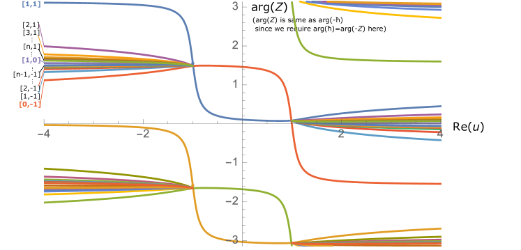
Figure 14: The BPS walls when we fix $\Lambda=1$ and ${\rm Im}(u)=\frac{{\rm i}}{10}$. The horizontal axis is ${\rm Re}(u)$. There are two special points around at $u_{1}\approx-1+\frac{{\rm i}}{10}$ and $u_{2}\approx 1+\frac{{\rm i}}{10}$ where the wall of marginal stability is encountered: $\arg(Z_{\gamma_{[1,1]}})=\arg(Z_{\gamma_{[0,-1]}})$. For ${\rm Re}(u)\in(u_{1},u_{2})$ (strong coupling) we have 2 hypermultiplets and their antiparticles, so there are 4 walls in total shown in this region. For ${\rm Re}(u)<{\rm Re}(u_{1})$ or ${\rm Re}(u)>{\rm Re}(u_{2})$ (weak coupling), we have infinitely many hypermultiplets. The hypermultiplet walls accumulate around the vectormultiplet wall. We list the electromagnetic charges of the particles next to their corresponding walls.

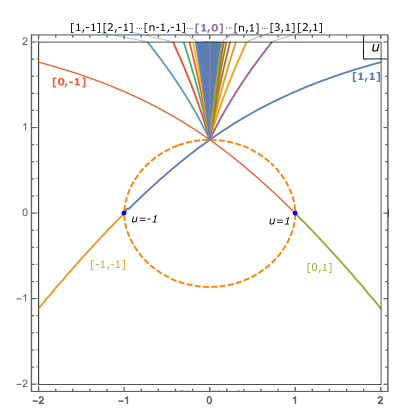
Figure 15: The $u$ plane for the pure $SU(2)$ SYM theory with $\Lambda=1$. The wall of marginal stability is shown as an orange dashed curve passing through the magnetic and dyonic singularities at $u=\pm 1$. We plot $\arg(Z_{\gamma}(u,\Lambda=1))=\pi/4$ for different $\gamma$. The notation $[i,j]$ stands for a path obeying $\arg(Z_{\gamma_{[i,j]}}(u,\Lambda=1))=\pi/4$. In the strong coupling region we have only two paths corresponding to $\arg(Z_{\gamma_{[0,-1]}}(u,\Lambda=1))=\pi/4$ and $\arg(Z_{\gamma_{[1,1]}}(u,\Lambda=1))=\pi/4$. Outside the wall of marginal stability, there is a vector multiplet $[1,0]$ and an infinite tower of hypermultiplets: $[n,-1]$ and $[n+1,1]$ with $n\geq 1$. These accumulate around $[1,0]$ when $n\rightarrow\infty$. At the boundaries of this infinite tower we have $[0,-1]$ and $[1,1]$.

C.2 Borel plane poles of WKB solutions

We have seen that in Section 3.4, the singularities in the Borel transform $\hat{Y}(z,\zeta)$ correspond to central charges of solitons on the surface defect parametrized by $z$. We want to test this also for the simpler example of the pure $SU(2)$ theory. In this case the relevant Schrödinger equation is (we take $\Lambda^{2}=1/2$)

$$(-\hbar^{2}\partial_{x}^{2}+\cosh x-2u)\psi(x)=0.$$ (C.5)

The results are shown in Figure 16 and Figure 17. We find perfect agreement with the statement presented in Section 3.4.

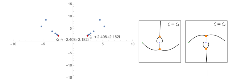
Figure 16: Left: singularities of the Padé-Borel transform of the ${Y}^{(2)}$ in (3.7) for the operator (C.5). We take $u=0$, $z=\operatorname{{\rm e}}^{x}=-\operatorname{{\rm e}}$ and use $N=40$ terms in the series. The leading singularities $\zeta_{i}$, marked in red, match well with (3.23); thus as expected they are the central charges of BPS solitons on the surface defect with parameter $z$. (For $Y^{(1)}$ the singularities would be at the opposite points $\zeta=-\zeta_{i}$.) Right: for fixed $\zeta=\zeta_{i}$ we plot a cutoff version of the Stokes graphs with $\vartheta=\arg(\zeta)$, plotting the Stokes curves only up to $|2\int_{z_{0}}^{z}\lambda|=\lvert\zeta\rvert$. As explained around (3.23), the cutoff Stokes curves $\mathcal{W}^{\vartheta=\arg(\zeta_{i})}$ run exactly up to the point $z=-\operatorname{{\rm e}}$, which is plotted as a green dot.

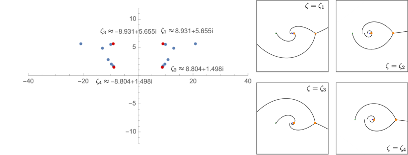
Figure 17: Left: singularities in the Padé-Borel transform of the ${Y}^{(2)}$ in (3.7) for the operator (C.5). We take $u=1$, $z=\operatorname{{\rm e}}^{x}=-\operatorname{{\rm e}}$ and use $N=40$ terms in the series. There are infinitely many poles of $\hat{Y}^{(2)}$, corresponding to the central charges of solitons on the surface defect parameterized by $z$. Only finitely many of them are visible in our approximation. (Again, for $Y^{(1)}$ the singularities would be at the opposite points $\zeta=-\zeta_{i}$.) Right: cutoff Stokes graphs at $\zeta=\zeta_{1},\zeta_{2},\zeta_{3},\zeta_{4}$, as in Figure 16 above.

C.3 Relation between Fock-Goncharov coordinates and Fenchel-Nielsen coordinates in the pure $SU(2)$ theory

In Section 7.2 we use the analytic continuation of exponentially decaying solutions, as well as the Wronskians expressions for the quantum periods, to relate Fock-Goncharov coordinates to Fenchel-Nielsen coordinates in the $SU(2)$ $N_{f}=1$ theory. This enables us to compare quantum periods gotten by instanton counting (which are Fenchel-Nielsen coordinates) with all the other Fock-Goncharov coordinates.

Here we work out the relation between Fock-Goncharov coordinates and Fenchel-Nielsen coordinates in the case of the pure $SU(2)$ theory.

For Fenchel-Nielsen coordinates we use the same spectral network $\mathcal{W}$ as in Hollands:2019wbr , this is shown in 18(a). More precisely, the Fenchel-Nielsen coordinates for the ring domain and the hypermultiplet are $\mathcal{X}^{\rm FN}_{\gamma_{e}/2}$ and $\mathcal{X}_{\gamma_{m}}^{\rm FN}$ respectively (see 18(a)). We also denote $\mathcal{X}_{\gamma_{h}}^{\rm FG}$ the Fock-Goncharov coordinate corresponding to the hypermultiplet shown in 18(b).

By using the spectral networks in Figure 18 we can obtain the Wronskian expressions for these coordinates . We get

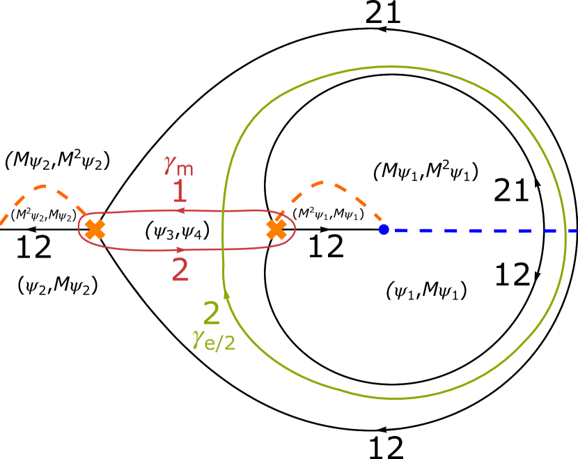
(a)

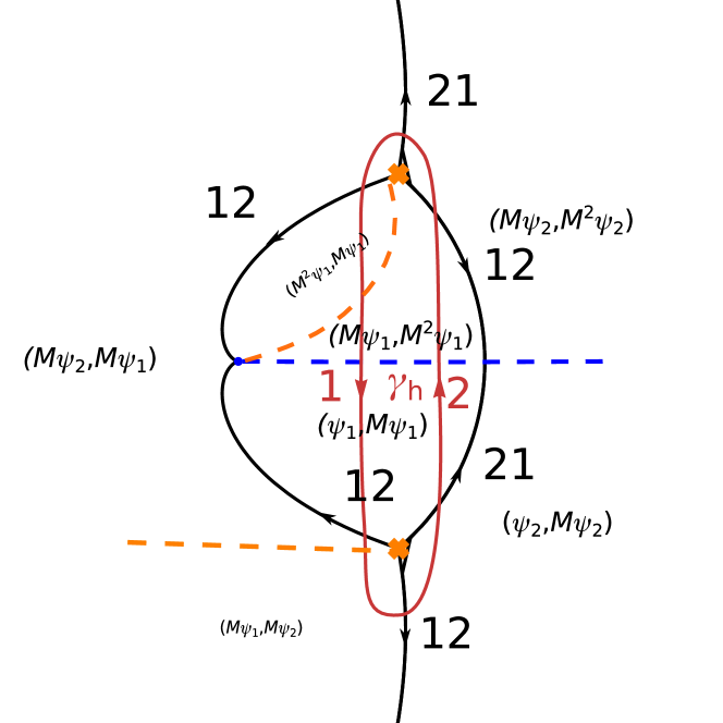
(b)

Figure 18: The spectral networks used for writing the Wronskians for Fenchel-Nielsen and Fock-Goncharov coordinates. The Seiberg-Witten curve is given in (C.1). In 18(a) we choose $\Lambda=1$, $u=-9/8$. In 18(b) we choose $\Lambda=1$, $u=13/20$.

$$\mathcal{X}^{\rm FN}_{\gamma_{e}/2}=\mu,$$ (C.6)

$$\mathcal{X}_{\gamma_{m}}^{\rm FN}=-\frac{[\psi_{1},\psi_{4}][\psi_{2},\psi_{3}]}{[\psi_{1},\psi_{3}][\psi_{2},\psi_{4}]}\,,$$ (C.7)

$$\mathcal{X}_{\gamma_{h}}^{\rm FG}=-\frac{[\psi_{1},M\psi_{1}][\psi_{2},M\psi_{2}]}{[\psi_{2},\psi_{1}]^{2}}\,$$ (C.8)

where $M\psi_{1}$ and $M\psi_{2}$ are the exponentially decaying solutions approaching $0^{-}$ and $-\infty$ respectively; we refer to Hollands:2019wbr for the details. Following the same techniques described in Section 7.2, we get

$$\mathcal{X}_{\gamma_{h}}^{\rm FG}=\frac{\sinh^{2}(\Pi^{\rm FN}_{\gamma_{e}}/2)}{\cosh^{2}(\Pi^{\rm FN}_{\gamma_{m}}/2)}.$$ (C.9)

Thus

$$\operatorname{{\rm e}}^{\Pi_{\gamma_{h}}^{\rm FG}/2}=\frac{\sinh(\Pi^{\rm FN}_{\gamma_{e}}/2)}{\cosh(\Pi^{\rm FN}_{\gamma_{m}}/2)},$$ (C.10)

up to a sign. This is precisely the relation obtained in (Grassi:2019coc, , eq. (5.44)) by comparing Fredholm determinant expressions with the TBA for quantum periods.

Appendix D Fredholm determinant: numerical tests

In this part we present some numerical test of formula (8.12) and its corollary (8.18).

We start by providing some tests of the quantization condition (8.18). Some results are shown in Table 5.

Nb	$E_{0}$
0	1.676395409 + 1.526799724 i
1	1.672311313 + 1.528945186 i
2	1.675315205 + 1.524899573 i
4	1.675315904 + 1.524888977 i
5	1.675315835 + 1.524889216 i
8	1.675315869 + 1.524889085 i
Num	1.67531587 + 1.52488909 i

Nb	$E_{0}$
0	4.398570612
1	4.308165565
3	4.303216550
5	4.303209956
6	4.303210145
8	4.303210165
Num	4.303210165

Table 5: First energy level of (8.11) for $\hbar=1$, $m=1/20$, $\Lambda=1$ (left) and $\hbar=1$, $m=2{\rm i}$, $\Lambda=\operatorname{{\rm e}}^{-{\rm i}\pi/6}$ (right). Nb denotes the order at which we truncate the instanton counting expression (6.1). The numerical value in the last line is obtained by using numerical diagonalization of the operator.

We now want to test the expression (8.12) for the Fredholm determinant. In principle we can compute the spectrum $E_{n}$ numerically and evaluate the full determinant $\prod_{n\geq 0}\left(1-{E\over E_{n}}\right)$ numerically. However this product converges a bit slow. Hence, from a numerical point of view, it is often more convenient to compute the spectral traces

$$Z_{\ell}=\operatorname{Tr}{\rm O}_{\rm 4d}^{-\ell}=\sum_{n\geq 0}{1\over E_{n}^{\ell}}.$$ (D.1)

These appear when we expand the Fredholm determinant at small $E$, namely

$$\det\left(1-{E\over{\rm O}_{4d}}\right)=\prod_{n\geq 0}\left(1-{E\over E_{n}}\right)=\sum_{N\geq 0}(-E)^{N}Z(N)$$ (D.2)

where the first few terms reads

$$Z(1)= Z_{1},$$ (D.3)

$$Z(2)= {1\over 2}\left(Z_{1}^{2}-Z_{2}\right),$$

$$Z(3)= \frac{1}{6}\left(Z_{1}^{3}-3Z_{2}Z_{1}+2Z_{3}\right),$$

$$Z(4)= \frac{1}{24}\left(Z_{1}^{4}-6Z_{2}Z_{1}^{2}+8Z_{3}Z_{1}+3Z_{2}^{2}-6Z_{4}\right),$$

$$\cdots$$

We call $Z(N)$ fermionic spectral traces to distinguish them from the standard spectral traces $Z_{\ell}$ defined in (D.1) . We can invert the above relation and find

$$Z_{1}= Z({1}),$$ (D.4)

$$Z_{2}= Z(1)^{2}-2Z(2),$$

$$Z_{3}= Z(1)^{3}-3Z(1)Z(2)+3Z(3),$$

$$Z_{4}= Z(1)^{4}-4Z(1)^{2}Z(2)+2Z(2)^{2}+4Z(1)Z(3)-4Z(3),$$

From a gauge/string theory perspective we can compute these traces analytically by using the expression on the r.h.s. of (8.12). More precisely we have

$$Z(N)=A(\hbar,{m},\Lambda){(-1)^{N}\over N!}{{\rm d}^{N}\over{\rm d}^{N}E}\left(\operatorname{{\rm e}}^{\frac{3}{8}{\tt a}}\operatorname{{\rm e}}^{{\tt a}_{m}\over 2}2\cosh\left({{\tt a}_{D}\over 2}\right)\right)\Big{|}_{E=0}.$$ (D.5)

In Table 6 we test that the specral traces computed numerically match with the analytic expression obtained from (D.5). Note that numerically it is hard to compute $Z_{1}$ and $Z_{2}$ because they converge quite slowly. Hence we compute $Z_{3}$ and $Z_{4}$.

Nb	$Z_{3}$	$Z_{4}$
1	24.02225295	66.8251024452
3	24.08424882	66.5241898596
5	24.08422501	66.5243963962
7	24.08422501	66.5243963159
Num	24.0842250	66.5243963159

Nb	$Z_{3}$
1	24.180623096276 - 59.7224031294781 i
3	24.168643262235 - 59.7212305226401 i
5	24.168642506932 - 59.7212305149533 i
7	24.168642506897 - 59.7212305149523 i
Num	24.16864250   - 59.721230515 i

Table 6: Left: the third and fourth spectral traces as computed from (D.5) for $m=0$, $\hbar=1$, $\Lambda=\frac{1}{5}\operatorname{{\rm e}}^{-\frac{1}{6}(i\pi)}$. Right: the third spectral trace as computed from (D.5) for $m=1/20$, $\hbar=1$, $\Lambda=\frac{1}{7}$. We denote by $\rm Nb$ the order at which we truncate the NS partition function (6.1). The numerical result is obtained by numerical diagonalization of the operator (8.11).

References

- (1) R. Balian, G. Parisi, and A. Voros, “Quartic oscillator,” in Feynman Path Integrals, vol. 106, pp. 337–360. Springer–Verlag, 1979.
- (2) A. Voros, “The return of the quartic oscillator. The complex WKB method,” Annales de l’I.H.P. Physique Théorique 39 (1983), no. 3, 211–338.
- (3) A. Voros, Spectre de l’équation de Schrödinger et méthode BKW. Publications Mathématiques d’Orsay, 1981.
- (4) E. Delabaere, H. Dillinger, and F. Pham, “Exact semiclassical expansions for one-dimensional quantum oscillators,” J. Math. Phys. 38 (1997), no. 12, 6126–6184.
- (5) H. Dillinger, E. Delabaere, and F. Pham, “Résurgence de Voros et périodes des courbes hyperelliptiques,” Annales de l’Institut Fourier 43 (1993) 163.
- (6) K. Iwaki and T. Nakanishi, “Exact WKB analysis and cluster algebras,” J. Phys. A 47 (2014), no. 47, 474009.
- (7) D. Gaiotto, “Opers and TBA,” 1403.6137.
- (8) L. Hollands and A. Neitzke, “Exact WKB and abelianization for the equation,” 1906.04271.
- (9) N. A. Nekrasov and S. L. Shatashvili, “Quantization of integrable systems and four dimensional gauge theories,” in 16th International Congress on Mathematical Physics, Prague, August 2009, 265-289, World Scientific 2010. 2009. 0908.4052.
- (10) N. Nekrasov, A. Rosly, and S. Shatashvili, “Darboux coordinates, Yang-Yang functional, and gauge theory,” Theor. Math. Phys. 181 (2014), no. 1, 1206–1234. [Erratum: Theor.Math.Phys. 182, 368 (2015)].
- (11) N. Nekrasov and E. Witten, “The Omega Deformation, Branes, Integrability, and Liouville Theory,” JHEP 09 (2010) 092, 1002.0888.
- (12) N. Drukker, J. Gomis, T. Okuda, and J. Teschner, “Gauge Theory Loop Operators and Liouville Theory,” JHEP 1002 (2010) 057, 0909.1105.
- (13) L. F. Alday, D. Gaiotto, S. Gukov, Y. Tachikawa, and H. Verlinde, “Loop and surface operators in N=2 gauge theory and Liouville modular geometry,” JHEP 01 (2010) 113, 0909.0945.
- (14) K. Maruyoshi and M. Taki, “Deformed Prepotential, Quantum Integrable System and Liouville Field Theory,” Nucl. Phys. B841 (2010) 388–425, 1006.4505.
- (15) S. Jeong and N. Nekrasov, “Opers, surface defects, and Yang-Yang functional,” 1806.08270.
- (16) A. Mironov and A. Morozov, “Nekrasov functions and exact Bohr–Sommerfeld integrals,” JHEP 1004 (2010) 040, 0910.5670.
- (17) A.-K. Kashani-Poor and J. Troost, “Pure super Yang–Mills and exact WKB,” JHEP 08 (2015) 160, 1504.08324.
- (18) Y. Emery, M. Mariño, and M. Ronzani, “Resonances and PT symmetry in quantum curves,” JHEP 04 (2020) 150, 1902.08606.
- (19) D. Dumas and A. Neitzke, “Opers and nonabelian Hodge: numerical studies,” 2007.00503.
- (20) K. Ito, M. Mariño, and H. Shu, “TBA equations and resurgent Quantum Mechanics,” JHEP 01 (2019) 228, 1811.04812.
- (21) K. Ito, S. Koizumi, and T. Okubo, “Quantum Seiberg-Witten curve and Universality in Argyres-Douglas theories,” Phys. Lett. B 792 (2019) 29–34, 1903.00168.
- (22) D. Fioravanti, H. Poghosyan, and R. Poghossian, “, and periods in SYM,” JHEP 03 (2020) 049, 1909.11100.
- (23) F. Yan, “Exact WKB and the quantum Seiberg-Witten curve for 4d pure Yang-Mills, Part I: Abelianization,” 2012.15658.
- (24) A. Grassi and M. Mariño, “A Solvable Deformation of Quantum Mechanics,” SIGMA 15 (2019) 025, 1806.01407.
- (25) Y. Hatsuda, A. Sciarappa, and S. Zakany, “Exact quantization conditions for the elliptic Ruijsenaars-Schneider model,” Journal of High Energy Physics 2018 (Nov, 2018).
- (26) K. Imaizumi, “Quantum periods and TBA equations for SQCD with flavor symmetry,” 2103.02248.
- (27) Y. Emery, “TBA Equations and Quantization Conditions,” 2008.13680.
- (28) G. Aminov, A. Grassi, and Y. Hatsuda, “Black Hole Quasinormal Modes and Seiberg-Witten Theory,” 2006.06111.
- (29) K. Ito, T. Kondo, K. Kuroda, and H. Shu, “WKB periods for higher order ODE and TBA equations,” 2104.13680.
- (30) D. Gaiotto, G. W. Moore, and A. Neitzke, “Four-dimensional wall-crossing via three-dimensional field theory,” Commun. Math. Phys. 299 (2010) 163–224, 0807.4723.
- (31) P. Dorey, C. Dunning, and R. Tateo, “The ODE/IM Correspondence,” J. Phys. A40 (2007) R205, hep-th/0703066.
- (32) N. Nikolaev, “Exact solutions for the singularly perturbed Riccati equation and exact WKB analysis,” 2008.06492.
- (33) D. Gaiotto, G. W. Moore, and A. Neitzke, “Wall-crossing, Hitchin Systems, and the WKB Approximation,” 0907.3987.
- (34) L. Hollands and A. Neitzke, “Spectral Networks and Fenchel–Nielsen Coordinates,” Lett. Math. Phys. 106 (2016), no. 6, 811–877, 1312.2979.
- (35) A. Grassi, J. Gu, and M. Mariño, “Non-perturbative approaches to the quantum Seiberg-Witten curve,” JHEP 07 (2020) 106, 1908.07065.
- (36) P. Dorey and R. Tateo, “Anharmonic oscillators, the thermodynamic Bethe ansatz, and nonlinear integral equations,” J. Phys. A 32 (1999) L419–L425, hep-th/9812211.
- (37) S. Codesido, A. Grassi, and M. Mariño, “Spectral theory and mirror curves of higher genus,” Annales Henri Poincaré 18 (2017), no. 2, 559–622, 1507.02096.
- (38) A. Grassi, Y. Hatsuda, and M. Mariño, “Topological strings from quantum mechanics,” Annales Henri Poincaré 17 (2016), no. 11, 3177–3235, 1410.3382.
- (39) M. Mariño, “Spectral Theory and Mirror Symmetry,” Proc. Symp. Pure Math. 98 (2018) 259, 1506.07757.
- (40) G. Bonelli, A. Grassi, and A. Tanzini, “Seiberg–Witten theory as a Fermi gas,” Lett. Math. Phys. 107 (2017), no. 1, 1–30, 1603.01174.
- (41) C. F. Doran, M. Kerr, and S. S. Babu, “ and quantum curves,” 2110.08482.
- (42) A. B. Zamolodchikov, “Generalized Mathieu equations and Liouville TBA,” in Quantum Field Theories in Two Dimensions, vol. 2. World Scientific, 2012.
- (43) L. Hollands and O. Kidwai, “Higher length-twist coordinates, generalized Heun’s opers, and twisted superpotentials,” Adv. Theor. Math. Phys. 22 (2018) 1713–1822, 1710.04438.
- (44) I. Coman, P. Longhi, and J. Teschner, “From quantum curves to topological string partition functions II,” 2004.04585.
- (45) D. Gaiotto, G. W. Moore, and A. Neitzke, “Wall-crossing in coupled 2d-4d systems,” JHEP 12 (2012) 1103.2598.
- (46) M. Aganagic, M. C. Cheng, R. Dijkgraaf, D. Krefl, and C. Vafa, “Quantum geometry of refined topological strings,” JHEP 1211 (2012) 019, 1105.0630.
- (47) R. Eager, S. A. Selmani, and J. Walcher, “Exponential Networks and Representations of Quivers,” JHEP 08 (2017) 063, 1611.06177.
- (48) P. Longhi, “On the BPS spectrum of 5d SU(2) super-Yang-Mills,” 2101.01681.
- (49) S. Banerjee, P. Longhi, and M. Romo, “Exploring 5d BPS Spectra with Exponential Networks,” 1811.02875.
- (50) S. Banerjee, P. Longhi, and M. Romo, “Exponential BPS graphs and D-brane counting on toric Calabi-Yau threefolds: Part II,” 2012.09769.
- (51) M. R. Douglas, B. Fiol, and C. Romelsberger, “The Spectrum of BPS branes on a noncompact Calabi-Yau,” JHEP 09 (2005) 057, hep-th/0003263.
- (52) C. Closset and M. Del Zotto, “On 5d SCFTs and their BPS quivers. Part I: B-branes and brane tilings,” 1912.13502.
- (53) G. Bonelli, F. Del Monte, and A. Tanzini, “BPS quivers of five-dimensional SCFTs, Topological Strings and q-Painlevé equations,” 2007.11596.
- (54) X. Wang, G. Zhang, and M.-x. Huang, “New exact quantization condition for toric Calabi–Yau geometries,” Phys. Rev. Lett. 115 (2015) 121601, 1505.05360.
- (55) M. Mariño and S. Zakany, “Exact eigenfunctions and the open topological string,” J. Phys. A50 (2017), no. 32, 325401, 1606.05297.
- (56) D. Gaiotto, G. W. Moore, and A. Neitzke, “Framed BPS States,” Adv. Theor. Math. Phys. 17 (2013), no. 2, 241–397, 1006.0146.
- (57) M. Kontsevich and Y. Soibelman, “Stability structures, motivic Donaldson-Thomas invariants and cluster transformations,” 0811.2435.
- (58) M. Kontsevich and Y. Soibelman, “Affine structures and non-Archimedean analytic spaces,” in The unity of mathematics, vol. 244 of Progr. Math., pp. 321–385. Birkhäuser Boston, Boston, MA, 2006.
- (59) M. Gross and B. Siebert, “From real affine geometry to complex geometry,” Ann. of Math. (2) 174 (2011), no. 3, 1301–1428.
- (60) T. Bridgeland, “Riemann–Hilbert problems from Donaldson–Thomas theory,” Inventiones mathematicae 216 (Dec, 2018) 69–124.
- (61) D. Gaiotto, G. W. Moore, and A. Neitzke, “Spectral networks,” Annales Henri Poincare 14 (2013) 1643–1731, 1204.4824.
- (62) E. Delabaere and F. Pham, “Resurgent methods in semi-classical asymptotics,” Annales de l’IHP 71 (1999) 1–94.
- (63) Y. Takei, “WKB analysis and Stokes geometry of differential equations,” in Analytic, algebraic and geometric aspects of differential equations, Trends Math., pp. 263–304. Birkhäuser/Springer, Cham, 2017.
- (64) T. Kawai and Y. Takei, Algebraic analysis of singular perturbation theory, vol. 227. American Mathematical Soc., 2005.
- (65) D. Gaiotto, “Surface Operators in N = 2 4d Gauge Theories,” JHEP 11 (2012) 090, 0911.1316.
- (66) S. Cecotti and C. Vafa, “On classification of supersymmetric theories,” Commun. Math. Phys. 158 (1993) 569–644, hep-th/9211097.
- (67) M.-x. Huang, “On gauge theory and topological string in Nekrasov–Shatashvili limit,” JHEP 06 (2012) 152, 1205.3652.
- (68) M.-x. Huang, A. Klemm, J. Reuter, and M. Schiereck, “Quantum geometry of del Pezzo surfaces in the Nekrasov-Shatashvili limit,” JHEP 02 (2015) 031, 1401.4723.
- (69) L. Hollands and A. Neitzke, “BPS states in the Minahan-Nemeschansky theory,” Commun. Math. Phys. 353 (2017), no. 1, 317–351, 1607.01743.
- (70) D. Fioravanti and D. Gregori, “Integrability and cycles of deformed gauge theory,” Phys. Lett. B 804 (2020) 135376, 1908.08030.
- (71) A. Braverman and P. Etingof, “Instanton counting via affine Lie algebras II: From Whittaker vectors to the Seiberg-Witten prepotential,” math/0409441.
- (72) Y. Zenkevich, “Nekrasov prepotential with fundamental matter from the quantum spin chain,” Phys. Lett. B701 (2011) 630–639, 1103.4843.
- (73) S. Codesido and M. Mariño, “Holomorphic Anomaly and Quantum Mechanics,” J. Phys. A51 (2018), no. 5, 055402, 1612.07687.
- (74) O. Lisovyy and A. Naidiuk, “Accessory parameters in confluent Heun equations and classical irregular conformal blocks,” 2101.05715.
- (75) G. Felder and M. Müller-Lennert, “Analyticity of Nekrasov Partition Functions,” Commun. Math. Phys. 364 (2018), no. 2, 683–718, 1709.05232.
- (76) M. A. Bershtein and A. I. Shchechkin, “q-deformed Painlevé function and q-deformed conformal blocks,” J. Phys. A50 (2017), no. 8, 085202, 1608.02566.
- (77) A. Its, O. Lisovyy, and Yu. Tykhyy, “Connection problem for the sine-Gordon/Painlevé III tau function and irregular conformal blocks,” Int. Math. Res. Notices 18 (2015) 8903–8924, 1403.1235.
- (78) A. Gorsky, A. Milekhin, and N. Sopenko, “Bands and gaps in Nekrasov partition function,” JHEP 01 (2018) 133, 1712.02936.
- (79) Y. Hatsuda, S. Moriyama, and K. Okuyama, “Instanton Effects in ABJM Theory from Fermi Gas Approach,” JHEP 01 (2013) 158, 1211.1251.
- (80) M. Matone, “Instantons and recursion relations in SUSY gauge theory,” Phys. Lett. B357 (1995) 342–348, hep-th/9506102.
- (81) R. Flume, F. Fucito, J. F. Morales, and R. Poghossian, “Matone’s relation in the presence of gravitational couplings,” JHEP 04 (2004) 008, hep-th/0403057.
- (82) S. Codesido, M. Mariño, and R. Schiappa, “Non-Perturbative Quantum Mechanics from Non-Perturbative Strings,” Annales Henri Poincare 20 (2019), no. 2, 543–603, 1712.02603.
- (83) A. Voros, “Zeta-regularisation for exact-WKB resolution of a general 1D Schrödinger equation,” 1202.3100.
- (84) A. Voros, “The zeta function of the quartic oscillator,” Nucl. Phys. B165 (1980) 209–236.
- (85) S. Codesido, A. Grassi, and M. Mariño, “Exact results in N=8 Chern-Simons-matter theories and quantum geometry,” JHEP 1507 (2015) 011, 1409.1799.
- (86) S. Codesido, J. Gu, and M. Mariño, “Operators and higher genus mirror curves,” JHEP 02 (2017) 092, 1609.00708.
- (87) A. Grassi and M. Mariño, “The complex side of the TS/ST correspondence,” J. Phys. A52 (2019), no. 5, 055402, 1708.08642.
- (88) S. H. Katz, A. Klemm, and C. Vafa, “Geometric engineering of quantum field theories,” Nucl.Phys. B497 (1997) 173–195, hep-th/9609239.
- (89) A. Klemm, W. Lerche, P. Mayr, C. Vafa, and N. P. Warner, “Selfdual strings and N=2 supersymmetric field theory,” Nucl. Phys. B477 (1996) 746–766, hep-th/9604034.
- (90) N. Nekrasov, “Five dimensional gauge theories and relativistic integrable systems,” Nucl. Phys. B531 (1998) 323–344, hep-th/9609219.
- (91) V. A. Fateev and S. L. Lukyanov, “Boundary RG flow associated with the AKNS soliton hierarchy,” J. Phys. A 39 (2006) 12889–12926, hep-th/0510271.
- (92) F. Ferrari and A. Bilal, “The Strong coupling spectrum of the Seiberg-Witten theory,” Nucl. Phys. B469 (1996) 387–402, hep-th/9602082.