Study of List-Based OMP and an Enhanced Model for Direction Finding with Non-Uniform Arrays

Abstract

This paper proposes an enhanced coarray transformation model (EDCTM) and a mixed greedy maximum likelihood algorithm called List-Based Maximum Likelihood Orthogonal Matching Pursuit (LBML-OMP) for direction-of-arrival estimation with non-uniform linear arrays (NLAs). The proposed EDCTM approach obtains improved estimates when Khatri-Rao product-based models are used to generate difference coarrays under the assumption of uncorrelated sources. In the proposed LBML-OMP technique, for each iteration a set of candidates is generated based on the correlation-maximization between the dictionary and the residue vector. LBML-OMP then chooses the best candidate based on a reduced-complexity asymptotic maximum likelihood decision rule. Simulations show the improved results of EDCTM over existing approaches and that LBML-OMP outperforms existing sparse recovery algorithms as well as Spatial Smoothing Multiple Signal Classification with NLAs.

I Introduction

There has been, recently, a great deal of research in the field of sparse reconstruction with Compressive Sensing (CS) algorithms. These techniques have been used for direction-of-arrival (DOA) estimation with several advantages over classical [1] and subspace techniques [2, 3, 4, 5, 6, 7, 8, 9, 10, 11, 12, 13, 14, 15, 16, 17, 18, 19, 20, 21, 22, 23, 24, 25, 26, 27, 28, 29, 30, 31, 32, 33] as they can cost-effectively perform this task in challenging scenarios with excellent performance [34, 35].

In [36], an approach for quasi-stationary signals was proposed to estimate more sources than sensors, relying on the vectorization operator to build-up a full-rank effective array manifold. This technique was modified to deal with stationary signals through the introduction of a subspace-based algorithm known as Spatial Smoothing Multiple Signal Classification (SS-MUSIC) [37, 38] that performs spatial smoothing on what we call difference coarray transformation model (DCTM) in this paper. The DCTM model assumes perfectly uncorrelated sources, but does not account for finite-sample effects introduced by the vectorization operation. In addition, a sparse formulation of DCTM was proposed to deal with non-uniform linear arrays (NLAs) [39].

This formulation allows the use of most CS algorithms such as Orthogonal Matching Pursuit (OMP) [40], Iterative Hard Thresholding (IHT) [41], and Compressive Sampling Matching Pursuit (CoSaMP) [42], but suffers from the same finite sample-effect observed in the model developed in [37]. More recently, algorithms that exploit the sparsity property of the DOA spectrum have been developed, e.g., Sparse Bayesian Learning (SBL) and Focused OMP (FOMP) [43, 44].

Regarding classical DOA estimation, an asymptotic maximum likelihood (ML) rule was developed in [45]. Despite being optimal from an estimation viewpoint in the mean-square sense, it is based on a nonlinear optimization procedure that is unfeasible for most practical scenarios with moderate to large number of source signals, since it requires a multi-dimensional grid search to find the optimal ML solution.

The objectives of this work are: i) to increase the accuracy of CS-based coarray DOA estimation with acceptable complexity when estimating support sets from deterministic largely coherent dictionaries; ii) to devise a cost-effective DOA estimation technique; and iii) to devise a novel coarray model that accounts for finite-sample errors in scenarios with uncorrelated sources and allows a more detailed analysis of the errors induced by the coarray transformation.

We propose an enhanced DCTM model (EDCTM) and a mixed greedy ML rule called List-Based Maximum Likelihood OMP (LBML-OMP) for DOA estimation with NLAs. The proposed EDCTM approach obtains improved angle estimates and emphasizes the errors introduced by Khatri-Rao product-based models for coarray DOA estimation with uncorrelated sources. In the case of LBML-OMP, a list of candidates is generated based on the correlation-maximization between the dictionary and the residue vector. The best candidate support set is then selected employing a modified reduced-complexity version of the asymptotic ML DOA estimator [45]. The intuition behind this is that a set of candidate atoms could result in a higher likelihood of selecting improved support set elements. Since we select one atom at a time, the set of candidates is reduced to only one element through an optimum rule that maximizes the likelihood. Simulations show the improved results of EDCTM over the standard coarray model and that LBML-OMP outperforms existing algorithms like OMP, IHT, CoSaMP, ROMP and SS-MUSIC.

Paper structure: In Section II, the data model for the DOA estimation problem with the standard difference coarray formulation is described. In Section III, the sparse version of this problem is presented so that it can be solved using CS, and the devised coarray model is described. In Section IV, the proposed LBML-OMP is detailed. In Section V, simulations are presented and discussed, whereas Section VI draws the conclusions.

Notation: $\mathbb{S}$, $a$, $\boldsymbol{\mathbf{a}}$ and $\boldsymbol{\mathbf{A}}$ indicate sets, scalars, column vectors, and matrices, respectively. $\boldsymbol{\mathbf{P}}_{\boldsymbol{\mathbf{A}}}=\boldsymbol{\mathbf{A}}(\boldsymbol{\mathbf{A}}^{H}\boldsymbol{\mathbf{A}})^{-1}\boldsymbol{\mathbf{A}}^{H}$ and $\boldsymbol{\mathbf{P}}_{\boldsymbol{\mathbf{A}}}^{\perp}=\boldsymbol{\mathbf{I}}-\boldsymbol{\mathbf{P}}_{\boldsymbol{\mathbf{A}}}$ are the projection matrices onto the range of $\boldsymbol{\mathbf{A}}$ and null-space of $\boldsymbol{\mathbf{A}}^{H}$. $\left\langle\boldsymbol{\mathbf{a}}\right\rangle_{\mathbb{L}}$ and $\left\langle\boldsymbol{\mathbf{A}}\right\rangle_{\mathbb{L}}$ are restrictions on the elements and the columns indexed by the set $\mathbb{L}$, respectively. For example, if $\mathbb{L}=\{3,4,1\}$ and $\boldsymbol{\mathbf{a}}=\left[5,-7,0,6\right]^{\top}$, then $\left\langle\boldsymbol{\mathbf{a}}\right\rangle_{\mathbb{L}}=\left[0,6,5\right]^{\top}\in\mathbb{C}^{\left|\mathbb{L}\right|}$. $\boldsymbol{\mathbf{A}}\circ\boldsymbol{\mathbf{B}}$ and $\boldsymbol{\mathbf{A}}\otimes\boldsymbol{\mathbf{B}}$ indicate the Khatri-Rao and Kronecker products, respectively. $\mathbb{S}\setminus\mathbb{L}$ denotes the difference between the sets $\mathbb{S}$ and $\mathbb{L}$. $\left\lvert\mathbb{D}\right\rvert$ is the cardinality of the set $\mathbb{D}$. $\left[N\right]$ and $[\boldsymbol{\mathbf{a}}]_{i}$ means the set $\left\{1,\ldots,N\right\}$ and the $i$-th entry of $\boldsymbol{\mathbf{a}}$, respectively.

II System Model and Problem Statement

Consider a linear array with $N$ sensors at normalized positions defined by the set of integers $\mathbb{S}$, illuminated by $D$ narrowband spatially and temporally uncorrelated sources with DOAs $\boldsymbol{\mathbf{\theta}}\in\mathbb{R}^{D}$ taken in relation to the array broadside axis. The received signal covariance matrix is given by [46, 47]

$$\boldsymbol{\mathbf{C}}_{\boldsymbol{\mathbf{x}}_{\mathbb{S}}}=\boldsymbol{\mathbf{A}}_{\mathbb{S}}\left(\boldsymbol{\mathbf{\theta}}\right)\operatorname{diag}\left[\sigma^{2}_{1},\ldots,\sigma^{2}_{D}\right]\boldsymbol{\mathbf{A}}_{\mathbb{S}}^{H}\left(\boldsymbol{\mathbf{\theta}}\right)+\sigma_{n}^{2}\boldsymbol{\mathbf{I}},$$ (2)

where $\boldsymbol{\mathbf{x}}_{\mathbb{S}}=\boldsymbol{\mathbf{A}}_{\mathbb{S}}(\boldsymbol{\mathbf{\theta}})\boldsymbol{\mathbf{s}}+\boldsymbol{\mathbf{n}}_{\mathbb{S}}\in\mathbb{C}^{N}$ is the received signal, $\boldsymbol{\mathbf{s}}\in\mathbb{C}^{D}$ is the vector of source signals, $\boldsymbol{\mathbf{n}}_{\mathbb{S}}\in\mathbb{C}^{N}$ is the noise vector, $\boldsymbol{\mathbf{A}}_{\mathbb{S}}(\boldsymbol{\mathbf{\theta}})$ is the array manifold matrix, $\boldsymbol{\mathbf{C}}_{\boldsymbol{\mathbf{x}}_{\mathbb{S}}}\in\mathbb{C}^{N\times N}$ is the received signal covariance matrix, $\boldsymbol{\mathbf{C}}_{\boldsymbol{\mathbf{s}}}=\operatorname{diag}\left[\sigma^{2}_{1},\ldots,\sigma^{2}_{D}\right]\in\mathbb{C}^{D\times D}$ is the uncorrelated zero-mean Gaussian sources covariance matrix, and $\boldsymbol{\mathbf{C}}_{\boldsymbol{\mathbf{n}}_{\mathbb{S}}}=\sigma_{n}^{2}\boldsymbol{\mathbf{I}}\in\mathbb{C}^{N\times N}$ represents the zero-mean additive white Gaussian noise covariance matrix. The source signals and the noise are assumed to be uncorrelated, and $\boldsymbol{\mathbf{C}}_{\boldsymbol{\mathbf{x}}_{\mathbb{S}}}$ can be estimated via the sample covariance matrix estimate denoted by $\hat{\boldsymbol{\mathbf{C}}}_{\boldsymbol{\mathbf{x}}_{\mathbb{S}}}$ [48].

An approach to increasing the available degrees of freedom of the array is the difference coarray transformation using the $\operatorname{vec}\left(\right)$ operator in (2), which allows us to obtain [49]

$$\operatorname{vec}\left(\boldsymbol{\mathbf{C}}_{\boldsymbol{\mathbf{x}}_{\mathbb{S}}}\right)=\left(\boldsymbol{\mathbf{A}}_{\mathbb{S}}^{\ast}\left(\boldsymbol{\mathbf{\theta}}\right)\circ\boldsymbol{\mathbf{A}}_{\mathbb{S}}\left(\boldsymbol{\mathbf{\theta}}\right)\right)\boldsymbol{\mathbf{p}}+\sigma_{n}^{2}\tilde{\boldsymbol{\mathbf{i}}},$$ (3)

where $\boldsymbol{\mathbf{p}}=\left[\sigma^{2}_{1},\ldots,\sigma^{2}_{D}\right]^{\top}$ contains the source signal powers and $\tilde{\boldsymbol{\mathbf{i}}}$ refers to the vectorization of $\boldsymbol{\mathbf{I}}$.

Define the vectors $\boldsymbol{\mathbf{a}}$ and $\boldsymbol{\mathbf{c}}$, such that $\left[\boldsymbol{\mathbf{a}}\right]_{k}=n_{k},~{}\forall~{}n_{k}\in\mathbb{S}$, $k\in\left[N\right]$, and $\boldsymbol{\mathbf{c}}=\boldsymbol{\mathbf{a}}\otimes\boldsymbol{\mathbf{1}}_{N}-\boldsymbol{\mathbf{1}}_{N}\otimes\boldsymbol{\mathbf{a}}$, where $\boldsymbol{\mathbf{1}}_{N}$ is the all-ones column vector of dimension $N$. Clearly, $\boldsymbol{\mathbf{c}}$ consists of all pairwise differences in the sensors normalized positions, with repetition among its entries. Suppose there is a set of indices $\mathbb{H}$ such that the indexing operation $\boldsymbol{\mathbf{c}}^{\prime}=\left\langle\boldsymbol{\mathbf{c}}\right\rangle_{\mathbb{H}}$ removes the repeated elements in $\boldsymbol{\mathbf{c}}$ after their first occurrence and sort them in ascending order. The entries of $\boldsymbol{\mathbf{c}}^{\prime}\in\mathbb{R}^{\left|\mathbb{D}\right|}$ define the set $\mathbb{D}$

$$\mathbb{D}=\left\{n_{i}-n_{k}|\left(n_{i},n_{k}\right)\in\mathbb{S}^{2}\text{, and }1\leq i,k\leq N\right\}$$ (4)

whose cardinality $\left|\mathbb{D}\right|$ is termed degrees of freedom (DoF). Notice that the set $\mathbb{H}$ is directly determined from the array geometry $\mathbb{S}$. Indexing both sides of (3) through $\mathbb{H}$, leads us to the DTCM model [37]:

$$\begin{split}\boldsymbol{\mathbf{x}}_{\mathbb{D}}&=\left[\begin{array}[]{@{}c|c@{}}\boldsymbol{\mathbf{A}}_{\mathbb{D}}(\boldsymbol{\mathbf{\theta}})&\boldsymbol{\mathbf{i}}\\ \end{array}\right]\left[\begin{array}[]{@{}c|c@{}}\boldsymbol{\mathbf{p}}^{\top}&\sigma_{n}^{2}\\ \end{array}\right]^{\top},\end{split}$$ (5)

where $\boldsymbol{\mathbf{A}}_{\mathbb{D}}\left(\boldsymbol{\mathbf{\theta}}\right)\in\mathbb{C}^{\textrm{DoF}\times D}$ is the coarray manifold matrix (row-indexing of $\boldsymbol{\mathbf{A}}_{\mathbb{S}}^{\ast}\left(\boldsymbol{\mathbf{\theta}}\right)\circ\boldsymbol{\mathbf{A}}_{\mathbb{S}}\left(\boldsymbol{\mathbf{\theta}}\right)\in\mathbb{C}^{N^{2}\times D}$ through $\mathbb{H}$), $\boldsymbol{\mathbf{x}}_{\mathbb{D}}\in\mathbb{C}^{\textrm{DoF}}$ is the coarray received signal, and $\left[\boldsymbol{\mathbf{i}}\right]_{k}=\delta(k-(\textrm{DoF}+1)/2)\in\left\{0,1\right\}^{\textrm{DoF}}$, for $k\in\left[\textrm{DoF}\right]$.

III Proposed Enhanced Model and CS-Based DOA Estimation

Consider a grid $\boldsymbol{\mathbf{\theta}}^{g}\in\mathbb{R}^{g}$ that contains the true DOAs $\boldsymbol{\mathbf{\theta}}$. The dense DTCM in (5) is cast with $\boldsymbol{\mathbf{\theta}}^{g}$ to include the $D$-sparse vector $\boldsymbol{\mathbf{p}}^{g}\in\mathbb{C}^{g}$ such that we obtain the sparse DCTM as [39]:

$$\begin{split}\boldsymbol{\mathbf{x}}_{\mathbb{D}}&=\left[\begin{array}[]{@{}c|c@{}}\boldsymbol{\mathbf{A}}_{\mathbb{D}}(\boldsymbol{\mathbf{\theta}}^{g})&\boldsymbol{\mathbf{i}}\\ \end{array}\right]\left[\begin{array}[]{@{}c|c@{}}\boldsymbol{\mathbf{p}}^{g\top}&\sigma_{n}^{2}\\ \end{array}\right]^{\top}\\ &=\boldsymbol{\mathbf{B}}\boldsymbol{\mathbf{h}},\text{ with }\lVert\boldsymbol{\mathbf{h}}\rVert_{0}\ll g+1,\end{split}$$ (6)

where $\boldsymbol{\mathbf{B}}\in\mathbb{C}^{\textrm{DoF}\times(g+1)}$ is the dictionary, $\boldsymbol{\mathbf{h}}\in\mathbb{C}^{g+1}$ is a $K$-sparse vector ($K=D+1$), and $\boldsymbol{\mathbf{x}}_{\mathbb{D}}$ is the measurement vector. We remark that the model in (6) is the sparse version of the DCTM model in (5).

III-A Proposed EDCTM model

In order to account for scenarios with finite snapshots that arise naturally in DOA estimation, an alternative to (5), termed Enhanced DCTM (EDCTM), has been devised as follows. From what has been previously explained, the model in (2) assumes spatially uncorrelated sources and noise. From that, $\boldsymbol{\mathbf{C_{s}}}$ is diagonal. This assumption makes the DCTM model simpler to compute. This is the formulation usually found in the literature [37, 49] and used to derive (5). However, evaluating (2) under a finite-snapshot perspective, it follows that $\hat{\boldsymbol{\mathbf{C}}}_{{\boldsymbol{\mathbf{x}}_{\mathbb{S}}}}\approx\boldsymbol{\mathbf{A}}_{\mathbb{S}}(\boldsymbol{\mathbf{\theta}})\hat{\boldsymbol{\mathbf{C}}}_{\boldsymbol{\mathbf{s}}}\boldsymbol{\mathbf{A}}_{\mathbb{S}}^{H}(\boldsymbol{\mathbf{\theta}})+\hat{\boldsymbol{\mathbf{C}}}_{\boldsymbol{\mathbf{n}}_{\mathbb{S}}}$, where the sources-noise crossed terms were removed because we are mainly interested in the finite-sample effect included in $\hat{\boldsymbol{\mathbf{C}}}_{\boldsymbol{\mathbf{s}}}$ and DCTM also does not account for these terms. The $\operatorname{vec}\left(\cdot\right)$ operator property $\operatorname{vec}\left(\boldsymbol{\mathbf{ABC}}\right)=\left(\boldsymbol{\mathbf{C}}^{T}\otimes\boldsymbol{\mathbf{A}}\right)\operatorname{vec}\left(\boldsymbol{\mathbf{B}}\right)$ allows us to write

$$\begin{split}\operatorname{vec}\left(\hat{\boldsymbol{\mathbf{C}}}_{{\boldsymbol{\mathbf{x}}_{\mathbb{S}}}}\right)&=\left(\boldsymbol{\mathbf{A}}_{\mathbb{S}}^{\ast}(\boldsymbol{\mathbf{\theta}})\otimes\boldsymbol{\mathbf{A}}_{\mathbb{S}}(\boldsymbol{\mathbf{\theta}})\right)\operatorname{vec}\left(\operatorname{diag}\left(\hat{\boldsymbol{\mathbf{C}}}_{\boldsymbol{\mathbf{s}}}\right)+\hat{\boldsymbol{\mathbf{C}}}_{\boldsymbol{\mathbf{s}}}\right.\\ &\left.-\operatorname{diag}\left(\hat{\boldsymbol{\mathbf{C}}}_{\boldsymbol{\mathbf{s}}}\right)\right)+\operatorname{vec}\left(\hat{\boldsymbol{\mathbf{C}}}_{\boldsymbol{\mathbf{n}}_{\mathbb{S}}}\right)\\ &=\left(\boldsymbol{\mathbf{A}}_{\mathbb{S}}^{\ast}(\boldsymbol{\mathbf{\theta}})\otimes\boldsymbol{\mathbf{A}}_{\mathbb{S}}(\boldsymbol{\mathbf{\theta}})\right)\operatorname{vec}\left(\operatorname{diag}\left(\hat{\boldsymbol{\mathbf{C}}}_{\boldsymbol{\mathbf{s}}}\right)\right)\\ &+\left(\boldsymbol{\mathbf{A}}_{\mathbb{S}}^{\ast}(\boldsymbol{\mathbf{\theta}})\otimes\boldsymbol{\mathbf{A}}_{\mathbb{S}}(\boldsymbol{\mathbf{\theta}})\right)\operatorname{vec}\left(\hat{\underline{\boldsymbol{\mathbf{C}}}}_{\boldsymbol{\mathbf{s}}}\right)+\operatorname{vec}\left(\hat{\boldsymbol{\mathbf{C}}}_{\boldsymbol{\mathbf{n}}_{\mathbb{S}}}\right)\\ &=\left(\boldsymbol{\mathbf{A}}_{\mathbb{S}}^{\ast}(\boldsymbol{\mathbf{\theta}})\circ\boldsymbol{\mathbf{A}}_{\mathbb{S}}(\boldsymbol{\mathbf{\theta}})\right)\operatorname{vecd}\left(\hat{\boldsymbol{\mathbf{C}}}_{\boldsymbol{\mathbf{s}}}\right)\\ &+\overbrace{\operatorname{vec}\left(\boldsymbol{\mathbf{A}}_{\mathbb{S}}(\boldsymbol{\mathbf{\theta}})\hat{\underline{\boldsymbol{\mathbf{C}}}}_{\boldsymbol{\mathbf{s}}}\boldsymbol{\mathbf{A}}_{\mathbb{S}}^{H}(\boldsymbol{\mathbf{\theta}})\right)}^{\begin{subarray}{c}\textrm{error term }\boldsymbol{\mathbf{\eta}}\end{subarray}}+\operatorname{vec}\left(\hat{\boldsymbol{\mathbf{C}}}_{\boldsymbol{\mathbf{n}}_{\mathbb{S}}}\right),\end{split}$$ (7)

where the error term is a function of the hollow matrix $\hat{\underline{\boldsymbol{\mathbf{C}}}}_{\boldsymbol{\mathbf{s}}}=\hat{\boldsymbol{\mathbf{C}}}_{\boldsymbol{\mathbf{s}}}-\operatorname{diag}\left(\hat{\boldsymbol{\mathbf{C}}}_{\boldsymbol{\mathbf{s}}}\right)$ and $\operatorname{vecd}(\cdot)$ is the linear diagonal extraction operator, which maps a matrix into a column vector with entries equal to the main diagonal elements, i.e., $\operatorname{vecd}\left(\hat{\boldsymbol{\mathbf{C}}}_{\boldsymbol{\mathbf{s}}}\right)=\sum_{i=1}^{D}\boldsymbol{\mathbf{P}}_{\boldsymbol{\mathbf{e}}_{i}}\hat{\boldsymbol{\mathbf{C}}}_{\boldsymbol{\mathbf{s}}}\boldsymbol{\mathbf{e}}_{i}$, where $\boldsymbol{\mathbf{P}}_{\boldsymbol{\mathbf{e}}_{i}}=\boldsymbol{\mathbf{e}}_{i}\boldsymbol{\mathbf{e}}_{i}^{T}$ stands for the orthogonal projection operator onto the one-dimensional space spanned by the canonical basis vector $\boldsymbol{\mathbf{e}}_{i}$. From (7), it follows that

$$\operatorname{vec}\left(\hat{\boldsymbol{\mathbf{C}}}_{{\boldsymbol{\mathbf{x}}_{\mathbb{S}}}}\right)-\boldsymbol{\mathbf{\eta}}=\left(\boldsymbol{\mathbf{A}}_{\mathbb{S}}^{\ast}(\boldsymbol{\mathbf{\theta}})\circ\boldsymbol{\mathbf{A}}_{\mathbb{S}}(\boldsymbol{\mathbf{\theta}})\right)\hat{\boldsymbol{\mathbf{p}}}+\operatorname{vec}\left(\hat{\boldsymbol{\mathbf{C}}}_{\boldsymbol{\mathbf{n}}_{\mathbb{S}}}\right).$$ (8)

Assuming $\left\langle\operatorname{vec}\left(\hat{\boldsymbol{\mathbf{C}}}_{\boldsymbol{\mathbf{n}}_{\mathbb{S}}}\right)\right\rangle_{\mathbb{H}}\approx\hat{\sigma}_{n}^{2}\boldsymbol{\mathbf{i}}$ and indexing both sides of (8) through $\mathbb{H}$, leads to the proposed dense EDCTM given by

$$\hat{\boldsymbol{\mathbf{x}}}_{\mathbb{D}}^{\rm EDCTM}=\hat{\boldsymbol{\mathbf{x}}}_{\mathbb{D}}-\boldsymbol{\mathbf{\eta}}^{\prime}=\left[\begin{array}[]{@{}c|c@{}}\boldsymbol{\mathbf{A}}_{\mathbb{D}}(\boldsymbol{\mathbf{\theta}})&\boldsymbol{\mathbf{i}}\\ \end{array}\right]\left[\begin{array}[]{@{}c|c@{}}\hat{\boldsymbol{\mathbf{p}}}^{\top}&\hat{\sigma}_{n}^{2}\\ \end{array}\right]^{\top},$$ (9)

with corresponding sparse version assuming the form ^x_D^EDCTM & =^x_D-η^′
= [A_D(θ^g)i][ ^p^g⊤^σ_n^2 ]^⊤
= B^h, with ∥^h ∥_0≪g+1, where $\boldsymbol{\mathbf{\eta}}^{\prime}=\left\langle\boldsymbol{\mathbf{\eta}}\right\rangle_{\mathbb{H}}$. This model represents the acquired data with more precision and can be used for coarray DOA estimation by CS-based or conventional algorithms, under the assumption of previous knowledge of $\boldsymbol{\mathbf{\eta}}^{\prime}$ or the availability of its estimated version given by $\hat{\boldsymbol{\mathbf{\eta}}}^{\prime}_{\Delta}$, where $\Delta$ is an estimation procedure. Besides, it brings the attention to the fact that an important error is introduced when transforming standard arrays into coarrays for finite-snapshot scenarios with uncorrelated sources.

III-B Asymptotic properties and statistical behavior of EDCTM

The main goal of EDCTM is to remove the finite sample effect from the coarray model introduced by the sample covariance matrix of uncorrelated sources. The notion that this effect is more prominent for small-sample scenarios becomes clear through the analysis of the asymptotic behavior of $\boldsymbol{\mathbf{\eta}}^{\prime}$ (number of snapshots $T$ increases indefinitely). In order to verify that, we proceed as follows.

The sample covariance matrix follows a complex Wishart statistical distribution, since the sources are assumed to be zero-mean multivariate complex Gaussian distributed [50], i.e., $\hat{\boldsymbol{\mathbf{C}}}_{\boldsymbol{\mathbf{s}}}\thicksim\mathcal{CW}_{D}(T,(1/T)\boldsymbol{\mathbf{C_{s}}})$, where D sources are considered, there are $T$ snapshots available (Complex Wishart degrees of freedom) and $\boldsymbol{\mathbf{C}}_{\boldsymbol{\mathbf{s}}}=\operatorname{diag}(\boldsymbol{\mathbf{p}})$ represents the source signals covariance matrix. The moments for the elements of $\hat{\boldsymbol{\mathbf{C}}}_{\boldsymbol{\mathbf{s}}}$ were obtained in [51] through the differentiation of the characteristic function of the random variables $\left[\boldsymbol{\mathbf{C}}_{\boldsymbol{\mathbf{s}}}\right]_{11},\ldots,\left[\boldsymbol{\mathbf{C}}_{\boldsymbol{\mathbf{s}}}\right]_{D,D},2\mathfrak{Re}\left\{\left[\boldsymbol{\mathbf{C}}_{\boldsymbol{\mathbf{s}}}\right]_{12}\right\},2\mathfrak{Im}\left\{\left[\boldsymbol{\mathbf{C}}_{\boldsymbol{\mathbf{s}}}\right]_{12}\right\},\ldots,$ $2\mathfrak{Re}\left\{\left[\boldsymbol{\mathbf{C}}_{\boldsymbol{\mathbf{s}}}\right]_{N-1,N}\right\},2\mathfrak{Im}\left\{\left[\boldsymbol{\mathbf{C}}_{\boldsymbol{\mathbf{s}}}\right]_{N-1,N}\right\}$, resulting in

$$\begin{split}\mathbb{E}\left\{\left[\hat{\boldsymbol{\mathbf{C}}}_{\boldsymbol{\mathbf{s}}}\right]_{ij}\right\}&=\left[\boldsymbol{\mathbf{C_{s}}}\right]_{ij},\\ \end{split}$$ (10)

and

$$\begin{split}\mathbb{E}\left\{\left[\hat{\boldsymbol{\mathbf{C}}}_{\boldsymbol{\mathbf{s}}}\right]_{ij}\left[\hat{\boldsymbol{\mathbf{C}}}_{\boldsymbol{\mathbf{s}}}\right]_{ji}\right\}&=\mathbb{E}\left\{\left[\hat{\boldsymbol{\mathbf{C}}}_{\boldsymbol{\mathbf{s}}}\right]_{ij}\left[\hat{\boldsymbol{\mathbf{C}}}_{\boldsymbol{\mathbf{s}}}\right]_{ij}^{\ast}\right\}\\ &=\mathbb{E}\left\{\left\lvert\left[\hat{\boldsymbol{\mathbf{C}}}_{\boldsymbol{\mathbf{s}}}\right]_{ij}\right\rvert^{2}\right\}\\ &=\left\lvert\left[\boldsymbol{\mathbf{C}}_{\boldsymbol{\mathbf{s}}}\right]_{ij}\right\rvert^{2}+\frac{1}{T}\left[\boldsymbol{\mathbf{C}}_{\boldsymbol{\mathbf{s}}}\right]_{ii}\left[\boldsymbol{\mathbf{C}}_{\boldsymbol{\mathbf{s}}}\right]_{jj}.\end{split}$$ (11)

From this, since $\left[\boldsymbol{\mathbf{C}}_{\boldsymbol{\mathbf{s}}}\right]_{ij}=0\;\forall\;i\neq j$, then from (10) we can state that $\mathbb{E}\left\{\hat{\underline{\boldsymbol{\mathbf{C}}}}_{\boldsymbol{\mathbf{s}}}\right\}=\boldsymbol{\mathbf{0}}$, which yields

$$\begin{split}\mathbb{E}\left\{\boldsymbol{\mathbf{\eta}}^{\prime}\right\}&=\mathbb{E}\left\{\left\langle\operatorname{vec}\left(\boldsymbol{\mathbf{A}}_{\mathbb{S}}(\boldsymbol{\mathbf{\theta}})\hat{\underline{\boldsymbol{\mathbf{C}}}}_{\boldsymbol{\mathbf{s}}}\boldsymbol{\mathbf{A}}_{\mathbb{S}}^{H}(\boldsymbol{\mathbf{\theta}})\right)\right\rangle_{\mathbb{H}}\right\}\\ &=\left\langle\operatorname{vec}\left(\boldsymbol{\mathbf{A}}_{\mathbb{S}}(\boldsymbol{\mathbf{\theta}})\mathbb{E}\left\{\hat{\underline{\boldsymbol{\mathbf{C}}}}_{\boldsymbol{\mathbf{s}}}\right\}\boldsymbol{\mathbf{A}}_{\mathbb{S}}^{H}(\boldsymbol{\mathbf{\theta}})\right)\right\rangle_{\mathbb{H}}\\ &=\boldsymbol{\mathbf{0}}.\end{split}$$ (12)

Notice that the expected value of $\boldsymbol{\mathbf{\eta}}^{\prime}$ does not depend on the number of snapshots. Moreover, from (11), the variance for the off-diagonal elements of $\hat{\underline{\boldsymbol{\mathbf{C}}}}_{\boldsymbol{\mathbf{s}}}$ is given by

$$\mathbb{E}\left\{\left\lvert\left[\hat{\underline{\boldsymbol{\mathbf{C}}}}_{\boldsymbol{\mathbf{s}}}\right]_{ij}\right\rvert^{2}\right\}=\frac{1}{T}\left[\boldsymbol{\mathbf{C}}_{\boldsymbol{\mathbf{s}}}\right]_{ii}\left[\boldsymbol{\mathbf{C}}_{\boldsymbol{\mathbf{s}}}\right]_{jj}\;\forall\;i\neq j,$$ (13)

which clearly states the inversely proportional dependence of this variance on the number of snapshots. Then, we have

$$\lim_{T\to\infty}\mathbb{E}\left\{\left\lvert\left[\hat{\underline{\boldsymbol{\mathbf{C}}}}_{\boldsymbol{\mathbf{s}}}\right]_{ij}\right\rvert^{2}\right\}=0,$$ (14)

i.e., the variance collapses to zero and the error term $\boldsymbol{\mathbf{\eta}}^{\prime}$ tends to not deviate from its expected value, i.e., the zero value. This explains why DCTM and EDCTM become the same model when enough data becomes available. This will be illustrated in Section V through numerical simulations.

Remark: Unlike the work of Koochakzadeh and Pal [52] in which the impact of off-diagonal terms of the source covariance matrix on the data vector is discussed, EDCTM is concerned with uncorrelated sources and deals with the more practical finite-sample effect of the source sample covariance matrix (few snapshots), whereas the model (3) in [52] is intended to be used with correlated signals and was developed under the ideal infinite-snapshot condition. Therefore, the off-diagonal terms, and thus the correction terms, have different statistical characterization.

IV Proposed LBML-OMP Algorithm

The OMP algorithm is one of the most used sparse recovery strategies in CS [40, 53, 54]. Its $i$-th iteration performs an atom search such that the maximum correlation between a given atom from the dictionary and the residual vector is found (correlation-maximization (corr-max) step), according to

$$j=\underset{\hat{j}}{\operatorname{argmax}}\left\{\left\lvert\left[\boldsymbol{\mathbf{F}}^{H}\left(\boldsymbol{\mathbf{y}}-\boldsymbol{\mathbf{Fu}}^{(i)}\right)\right]_{\hat{j}}\right\rvert\right\},$$ (15)

where $\boldsymbol{\mathbf{y}}$ is the measurement vector, $\boldsymbol{\mathbf{F}}$ is the dictionary, and $\boldsymbol{\mathbf{u}}$ is the $K$-sparse vector to be found. Indeed, for scenarios with low SNR and few snapshots available, the OMP choice is not necessarily correct. The rationale is that, due to the nature of the deterministic dictionary, the neighbors of the OMP choice altogether increase the probability of containing the right solution.

The first step of LBML-OMP consists of a corr-max performed in the atoms indexed by $\mathbb{J}=\left[g\right]\setminus\mathbb{T}^{(i)}$, where $\mathbb{T}^{(i)}$ is the support set from the previous iteration. This prevents an atom from being selected twice. Consider the index $n_{0}$ such that $j=\left[\mathbb{J}\right]_{n_{0}}$, which is a restriction on $\mathbb{J}$ to the element indexed by $n_{0}$. From that, the set with candidate indices is compactly represented by $\mathbb{V}=\left\{\left[\mathbb{J}\right]_{n_{0}-n}~{}\biggl{\lvert}~{}n=\left\lfloor-\frac{Q-1}{2}\right\rfloor,\ldots,\left\lceil\frac{Q-1}{2}\right\rceil\right\}$, where $Q$ candidates are considered and $\left\lfloor\cdot\right\rfloor$ / $\left\lceil\cdot\right\rceil$ are the floor and ceil functions, respectively. In simple terms, $\mathbb{V}$ consists of the Q nearest neighbours on $\mathbb{J}$ around $j$ (OMP index estimate), including $j$ itself.

The candidate support sets for $\boldsymbol{\mathbf{p}}^{g}$ are given by the union of each of the elements in $\mathbb{V}$ with the support set from the previous iteration excluding the element $\left\{g+1\right\}$, i.e., $\mathbb{Y}_{q}=\left\{W_{N-1}\left(\mathbb{T}^{(i)}\right)\setminus\left\{g+1\right\}\right\}\cup v_{q}$, where $v_{q}\in\mathbb{V}$, $q\in[Q]$ and the $W_{N-1}(\cdot)$ operator keeps only the $N-1$ latest elements added to a given set. After the support sets $\mathbb{Y}_{q}$ are obtained, an optimum score rule must be devised to select the best possible approximation to the true DOAs $\boldsymbol{\mathbf{\theta}}$. A modified version of the asymptotic ML rule devised in [1, 45] is employed to perform this optimization procedure. Departing from zero-mean Gaussian complex sources, with i.i.d snapshots, the maximization of the log-likelihood function leads us to

$$\underset{\boldsymbol{\mathbf{\theta}},\boldsymbol{\mathbf{C}}_{\boldsymbol{\mathbf{s}}},\sigma_{n}^{2}}{\operatorname{maximize}}\quad-\left[\ln\operatorname{det}\left(\boldsymbol{\mathbf{C}}_{\boldsymbol{\mathbf{x}}_{\boldsymbol{\mathbf{\mathbb{S}}}}}\right)+\operatorname{tr}\left[\boldsymbol{\mathbf{C}}_{\boldsymbol{\mathbf{x}}_{\boldsymbol{\mathbf{\mathbb{S}}}}}^{-1}\hat{\boldsymbol{\mathbf{C}}}_{\boldsymbol{\mathbf{x}}_{\boldsymbol{\mathbf{\mathbb{S}}}}}\right]\right],$$ (16)

which has a separable solution for $\sigma_{n}^{2}$ and $\boldsymbol{\mathbf{C}}_{\boldsymbol{\mathbf{s}}}$. This solution can be used to obtain explicit functions of $\boldsymbol{\mathbf{\theta}}$. Replacing these functions into (16) we obtain the asymptotic (stochastic) ML estimator. After that, its D-dimensional domain is transformed into the domain built up by the candidates of the list. The rule for the optimum candidate selection becomes

$$\hat{q}\leftarrow\underset{q\in[Q]}{\operatorname{argmin}}\left\{\operatorname{det}\left(\boldsymbol{\mathbf{U}}_{q}\hat{\boldsymbol{\mathbf{C}}}_{\boldsymbol{\mathbf{x}}_{\mathbb{S}}}\boldsymbol{\mathbf{U}}_{q}+\frac{\operatorname{tr}\left(\boldsymbol{\mathbf{U}}_{q}^{\perp}\hat{\boldsymbol{\mathbf{C}}}_{\boldsymbol{\mathbf{x}}_{\mathbb{S}}}\right)}{N-\lvert\mathbb{Y}_{q}\rvert}\boldsymbol{\mathbf{U}}_{q}^{\perp}\right)\right\},$$ (17)

where $\boldsymbol{\mathbf{U}}_{q}=\boldsymbol{\mathbf{P}}_{\left\langle\boldsymbol{\mathbf{A}}_{\mathbb{S}}\left(\boldsymbol{\mathbf{\theta}}^{g}\right)\right\rangle_{\mathbb{Y}_{q}}}$. From that, the $\hat{q}$-th element of $\mathbb{V}$ is selected after a one-dimensional search on $Q$ points and its corresponding index $v_{\hat{q}}$ is added to the target support set. The $W_{N-1}(\cdot)$ operator plays the role of ensuring that the over the grid array manifold $\boldsymbol{\mathbf{A}}_{\mathbb{S}}\left(\boldsymbol{\mathbf{\theta}}^{g}\right)$ with atoms indexed by $\mathbb{Y}_{q}$ is full-column rank, thus allowing the appropriate calculus of the projection matrix $\boldsymbol{\mathbf{U}}_{q}$ and LBML-OMP to estimate more sources than sensors.

The estimated K-sparse solution is obtained through the orthogonal projection of $\boldsymbol{\mathbf{x}}_{\mathbb{D}}$ onto the spanning of the columns of $\boldsymbol{\mathbf{B}}$ indexed by the new target support set. This corresponds to the best possible $\mathbb{T}^{(i+1)}$-sparse approximation to the solution of (6) in the sense of the $l_{2}$-norm and can be obtained through

$$\boldsymbol{\mathbf{h}}^{(i+1)}=\underset{\boldsymbol{\mathbf{z}}\in\mathbb{C}^{g+1}}{\operatorname{argmin}}\left\{\lVert\boldsymbol{\mathbf{x}}_{\mathbb{D}}-\boldsymbol{\mathbf{\boldsymbol{\mathbf{Bz}}}}\rVert_{2}\textrm{, }\operatorname{supp}\left(\boldsymbol{\mathbf{z}}\right)\subset\mathbb{T}^{(i+1)}\right\},$$ (18)

After $K$ iterations, the final DOA estimates are obtained according to $\hat{\boldsymbol{\mathbf{\theta}}}=\left\langle\boldsymbol{\mathbf{\theta}}^{g}\right\rangle_{\mathbb{T}^{(K)}\setminus\left\{g+1\right\}}$. The LBML-OMP algorithm is summarized in Algorithm 1.

1

Input : dictionary $\boldsymbol{\mathbf{B}}\in\mathbb{C}^{\textrm{DoF}\times(g+1)}$, observed data $\boldsymbol{\mathbf{x}}_{\mathbb{D}}\in\mathbb{C}^{DoF}$, sparsity level $K=D+1$, array manifold matrix over the grid $\boldsymbol{\mathbf{A}}_{\mathbb{S}}\left(\boldsymbol{\mathbf{\theta}}^{g}\right)\in\mathbb{C}^{N\times g}$, sample received signal covariance matrix $\hat{\boldsymbol{\mathbf{C}}}_{\boldsymbol{\mathbf{x}}_{\mathbb{S}}}\in\mathbb{C}^{N\times N}$, number of sensors $N$, number of candidates $Q$, grid $\boldsymbol{\mathbf{\theta}}^{g}\in\mathbb{R}^{g}$

2

3$\mathbb{T}^{(0)}=\left\{g+1\right\}$, $\boldsymbol{\mathbf{h}}^{(0)}=\boldsymbol{\mathbf{0}}$

4for $i\leftarrow 0$ to $K-1$ do

5       $\mathbb{J}\leftarrow\left[g\right]\setminus\mathbb{T}^{(i)}$

6       $j^{(i)}\leftarrow\underset{\hat{j}\in\mathbb{J}}{\operatorname{argmax}}\left\{\left\lvert\left[\boldsymbol{\mathbf{B}}^{H}\left(\boldsymbol{\mathbf{x}}_{\mathbb{D}}-\boldsymbol{\mathbf{Bh}}^{(i)}\right)\right]_{\hat{j}}\right\rvert\right\}$

7       $n_{0}\leftarrow$ position index of $j^{(i)}$ in $\mathbb{J}$

8       $\mathbb{V}=\left\{\left[\mathbb{J}\right]_{n_{0}-n}~{}\bigl{\lvert}~{}n=\left\lfloor-\frac{Q-1}{2}\right\rfloor,\ldots,\left\lceil\frac{Q-1}{2}\right\rceil\right\}$

9       for $q\leftarrow 1$ to $Q$ do

10             $v_{q}\leftarrow q$-th element of the set $\mathbb{V}$

11             $\mathbb{Y}_{q}=\left\{W_{N-1}\left(\mathbb{T}^{(i)}\right)\setminus\left\{g+1\right\}\right\}\cup v_{q}$

12             $\boldsymbol{\mathbf{U}}_{q}\leftarrow\boldsymbol{\mathbf{P}}_{\left\langle\boldsymbol{\mathbf{A}}_{\mathbb{S}}\left(\boldsymbol{\mathbf{\theta}}^{g}\right)\right\rangle_{\mathbb{Y}_{q}}}$

13            

14      

15      $\hat{q}\leftarrow\underset{q\in[Q]}{\operatorname{argmin}}\left\{\operatorname{det}\left(\boldsymbol{\mathbf{U}}_{q}\hat{\boldsymbol{\mathbf{C}}}_{\boldsymbol{\mathbf{x}}_{\mathbb{S}}}\boldsymbol{\mathbf{U}}_{q}+\frac{\operatorname{tr}\left(\boldsymbol{\mathbf{U}}_{q}^{\perp}\hat{\boldsymbol{\mathbf{C}}}_{\boldsymbol{\mathbf{x}}_{\mathbb{S}}}\right)}{N-\lvert\mathbb{Y}_{q}\rvert}\boldsymbol{\mathbf{U}}_{q}^{\perp}\right)\right\}$

16       $\mathbb{T}^{(i+1)}\leftarrow\mathbb{T}^{(i)}\cup\left\{v_{\hat{q}}\right\}$

17       $\boldsymbol{\mathbf{h}}^{(i+1)}\leftarrow\underset{\boldsymbol{\mathbf{z}}\in\mathbb{C}^{g+1}}{\operatorname{argmin}}\left\{\lVert\boldsymbol{\mathbf{x}}_{\mathbb{D}}-\boldsymbol{\mathbf{\boldsymbol{\mathbf{Bz}}}}\rVert_{2}\textrm{, }\operatorname{supp}\left(\boldsymbol{\mathbf{z}}\right)\subset\mathbb{T}^{(i+1)}\right\}$

18      

19$\hat{\boldsymbol{\mathbf{\theta}}}\leftarrow\left\langle\boldsymbol{\mathbf{\theta}}^{g}\right\rangle_{\mathbb{T}^{(K)}\setminus\left\{g+1\right\}}$

Output : Estimated DOAs $\hat{\boldsymbol{\mathbf{\theta}}}$

Algorithm 1 Proposed LBML-OMP Algorithm

The asymptotic ML rule for DOA estimation, despite being optimum in the mean-square sense, is a commonly unfeasible approach for most practical scenarios with moderate to large numbers of source signals, if used in the way presented in the literature [1]. The reason for that lies in the requirement of its evaluation over a $D$-dimensional grid search. Instead, the devised approach in (17) requires a one-dimensional evaluation over only $Q$ points.

According to [55], the computational complexity of OMP is $\mathcal{O}\left(K\textrm{DoF}(g+1)\right)$, under the model in (6). The dominant stage is the computation of the pseudoinverse (projection). In the case of LBML-OMP, the whole process is similar, except for the projections $\boldsymbol{\mathbf{U}}_{q}$ (most costly part). Evaluating (17) for each candidate support has about the same complexity as that of one OMP iteration, which leads to a total complexity $Q+1$ times higher than that of OMP, i.e., $\mathcal{O}\left((Q+1)K\textrm{DoF}(g+1)\right)$.

V Simulation Results and Discussion

In the simulations, we consider the Uniform Linear Array (ULA), Two-Level Nested Array (NAQ2), 2nd-Order Super Nested Array (SNAQ2), Minimum Hole Array (MHA), and Minimum Redundancy Array (MRA) [56, 47, 38, 57, 58] schemes. In the performance evaluation, we employ the Optimal Sub-Pattern Assignment (OSPA) [59] metric given by

$$\begin{split}&\textrm{OSPA}(\hat{\boldsymbol{\mathbf{\theta}}},\boldsymbol{\mathbf{\theta}})=\\ &\sqrt{\frac{1}{LD}\sum_{l=1}^{L}\left(\underset{\mathbb{P}\in\mathbb{P}_{D}}{\operatorname{min}}\sum_{d=1}^{\hat{D}}g^{\left(\phi\right)}\left([\hat{\boldsymbol{\mathbf{\theta}}}]_{d}^{l},\left[\left\langle\boldsymbol{\mathbf{\theta}}\right\rangle_{\mathbb{P}}\right]_{d}\right)\right)^{2}+\phi^{2}\left(D-\hat{D}\right)},\end{split}$$ (19)

where $[\hat{\boldsymbol{\mathbf{\theta}}}]_{d}^{l}$ is $d$-th source DOA estimate for the $l$-th trial, $L$ is the total number of trials, $D$ is the total number of DOAs to be estimated, $\mathbb{P}_{D}$ denotes the set of permutations on $[D]$, $g^{(\phi)}(\hat{\theta},\theta)=\operatorname{min}(\phi,|\hat{\theta}-\theta|)$, and $\phi$ is a penalty parameter for the individual direction estimate and enumeration bias. The set of simulation parameters are shown in Table I, which contains the number of sensors, the number of trials for each figure, the normalized inter-sensor spacing, the grid dimension, the number of candidates for LBML-OMP, as well as the OSPA penalty parameter. The DOAs assume the values -0.3426$\pi$, -0.2947$\pi$, -0.2889$\pi$, -0.2820$\pi$, 0.2947$\pi$ radians, intentionally close to each other to assess the performance of the algorithms.

TABLE I: Set of Parameters

N (sensors)	L (trials)	$\nu/\lambda$ (sensor spacing)
8	5,000 (Fig. 1, 2, 4, and 6)     50,000 (Fig. 3 and 5)	1/2
g (grid dimension)	Q (number of candidates)	$\phi$ (OSPA penalty)
1024	11	0.0430

For the case that $\hat{D}>D$, $\textrm{OSPA}(\hat{\boldsymbol{\mathbf{\theta}}},\boldsymbol{\mathbf{\theta}})=\textrm{OSPA}(\boldsymbol{\mathbf{\theta}},\hat{\boldsymbol{\mathbf{\theta}}})$. This metric is similar to RMSE, but it allows the assessment of the error when the number of sources is not correctly estimated, usually employed in multi-target tracking. The number of candidates was set to $Q=11$. First, we analyze the behavior of LBML-OMP and then evaluate the EDCTM model.

V-A LBML-OMP

Consider the OSPA curves against SNR in Fig. 1 using an SNAQ2 arrangement under the DCTM model. Notice that for almost all the SNR range the devised strategy outperforms classical CS algorithms like IHT [41], CoSaMP, [42], and the more recently developed Sparse Bayesian Learning (SBL) [43], as well as coarray dense approaches like SS-MUSIC. Observe also that LBML-OMP is more costly than those algorithms, except SBL, but leads to increased accuracy due to the selection of candidates following an optimum rule.

At this point, we emphasize that the optimum ML rule in its original version is known to asymptotically achieve the Cramèr-Rao Lower Bound (CRLB) and is asymptotically unbiased (asymptotically efficient DOA estimator) [1, 45]. Thus, given an angular sector that comprises the uncertainty region (candidates list) for the OMP response, the derived extended ML rule performs the candidate selection reducing local errors in a feasible way. This rule reduces the potential mismatch between the OMP guess and the right support set element. In this way, it benefits from the synergy between CS-based DOA estimators and asymptotically optimum statistical estimators at the same time.

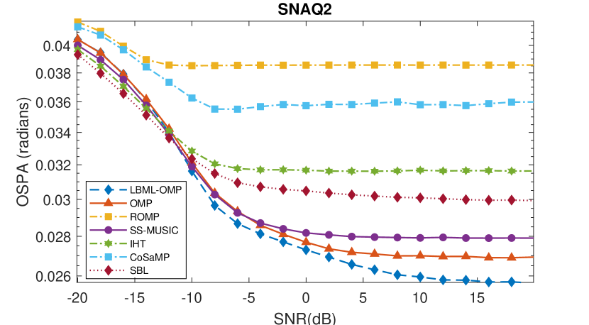
Figure 1: OSPA against SNR with SNAQ2 geometry for LBML-OMP, OMP, ROMP, SS-MUSIC, IHT, CoSaMP and SBL. $T=50$ snapshots.

Fig. 2 shows a comparison among the OSPA curves for LBML-OMP under several geometries: four non-uniform structures (NAQ2, SNAQ2, MHA and MRA) and a ULA. For this case, the arrays are considered to suffer from electromagnetic (EM) coupling. To this end, the B-banded coupling model described in [47], given by

$$\boldsymbol{\mathbf{x}}_{\mathbb{S}}^{\prime}=\boldsymbol{\mathbf{G}}\boldsymbol{\mathbf{A}}_{\mathbb{S}}(\boldsymbol{\mathbf{\theta}})\boldsymbol{\mathbf{s}}+\boldsymbol{\mathbf{n}}_{\mathbb{S}},$$ (20)

was employed, where $\boldsymbol{\mathbf{x}}_{\mathbb{S}}^{\prime}\in\mathbb{C}^{N}$ is the distorted received signal and $\boldsymbol{\mathbf{G}}\in\mathbb{C}^{N\times N}$ is the mutual coupling matrix with elements given by

$$\left[\boldsymbol{\mathbf{G}}\right]_{l,m}=\begin{dcases}g\left(\left\lvert n_{l}-n_{m}\right\rvert\right)&\text{if $\left\lvert n_{l}-n_{m}\right\rvert\leq B$},\\ 0&\text{otherwise}.\\ \end{dcases}$$ (21)

The coupling coefficients were derived from $g(k)=g(1)\exp(-j(k-1)\pi)/k$, for $2\leq k\leq B$, $B=100$ and $g(1)=0.3\exp\left(j\pi/3\right)$. The algorithms do not have any information about the matrix $\boldsymbol{\mathbf{G}}$. In Fig. 2, it is clear that MHA is the geometry with best performance for use with LBML-OMP. However, MHA as well as MRA do not have a closed-form solution for the positioning of sensors [1, 47]. Due to that, LBML-OMP can alternatively be employed with SNAQ2, the array with best results following MHA/MRA for most of the SNR range. In addition, it is worth mentioning that ULA exhibits the worst performance, justifying the use of non-uniform arrays for DOA estimation with the proposed approach. In Fig. 3 we demonstrate the LBML-OMP capability of identifying more sources than sensors ($N=8$ sensors and $D=10$ sources), due to the use of projection matrices that projects the coarray measurements into a full-column rank array manifold even for that condition.

Figure 2: OSPA against SNR for the proposed LBML-OMP with multiple geometries: ULA, SNAQ2, NAQ2, MRA, and MHA. $T=50$ snapshots.

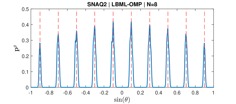
Figure 3: Identifying more sources than sensors. $N=8$ sensors and $D=10$ sources. $\boldsymbol{\mathbf{p}}^{g}$ against the sine of the sources DOAs with SNAQ2 geometry for LBML-OMP. Sine of sources DOAs uniformly spaced from -0.9 to 0.9. SNR$=20$ dB. $T=200$ snapshots.

V-B EDCTM

In Fig. 4, curves named with the suffix “_E” indicate the use of EDCTM, while its absence means that DCTM was employed. Clearly, EDCTM enhances the estimation performance of all algorithms as compared to the performance with the standard DCTM. Notice that EDCTM is also important for theoretical reasons because it might help to improve theoretical results in error analysis of coarray models. The improvement is more prominent for few snapshots and the models converge to the same response after enough data becomes available, according to what was discussed in Section III.

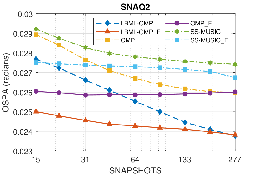
Figure 4: OSPA against snapshots with SNAQ2 geometry for OMP, LBML-OMP and SS-MUSIC using EDCTM (appended by “_E”) and DCTM. SNR$=10$ dB.

The statistical and asymptotic properties of EDCTM derived in Subsection III-B are illustrated in Fig. 5. For that, we have obtained the empirical pdf’s for the imaginary and real parts of $\left[\boldsymbol{\mathbf{\eta}}^{\prime}\right]_{1}$ for two cases: $T=350$ and $T=650$ snapshots. Moreover, we have also simulated its variance, i.e., $\mathbb{E}\left\{\left\lvert\left[\boldsymbol{\mathbf{\eta}}^{\prime}\right]_{1}\right\rvert^{2}\right\}$. Note that the mean of $\left[\boldsymbol{\mathbf{\eta}}^{\prime}\right]_{1}$ is indeed 0 for both imaginary and reals parts, and it does not depend on the number of snapshots. On the contrary, its variance is largely dependent on the amount of available data and tends to zero as we increase the number of snapshots. These conclusions agree with the theoretical analysis conducted in Subsection III-B.

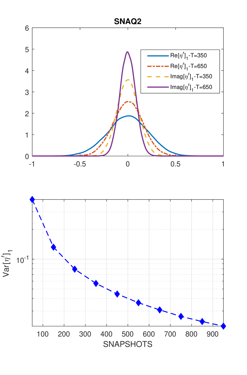
Figure 5: Statistical and asymptotic properties of $\left[\boldsymbol{\mathbf{\eta}}^{\prime}\right]_{1}$. Top: empirical pdf for $\mathfrak{Re}\left\{\left[\boldsymbol{\mathbf{\eta}}^{\prime}\right]_{1}\right\}$ and $\mathfrak{Im}\left\{\left[\boldsymbol{\mathbf{\eta}}^{\prime}\right]_{1}\right\}$ for $T=350$ and $T=650$ snapshots. Bottom: variance of $\left[\boldsymbol{\mathbf{\eta}}^{\prime}\right]_{1}$ against snapshots. SNR$=10$ dB.

To evaluate the effects of an estimated $\boldsymbol{\mathbf{\eta}}^{\prime}$, denoted by $\hat{\boldsymbol{\mathbf{\eta}}}^{\prime}$, we proceed as follows. Assume that $\hat{\boldsymbol{\mathbf{\eta}}}^{\prime}$ is obtained by an estimator $\Delta$. In this case,

$$\hat{\boldsymbol{\mathbf{\eta}}}^{\prime}_{\Delta}=\boldsymbol{\mathbf{\eta}}^{\prime}+\tilde{\boldsymbol{\mathbf{\eta}}}^{\prime},$$ (22)

where $\tilde{\boldsymbol{\mathbf{\eta}}}^{\prime}$ is an additive zero-mean white circular complex Gaussian distributed random vector (estimation error) with covariance matrix $\boldsymbol{\mathbf{C}}_{\tilde{\boldsymbol{\mathbf{\eta}}}^{\prime}}=\mathbb{E}\left\{\tilde{\boldsymbol{\mathbf{\eta}}}^{\prime}\tilde{\boldsymbol{\mathbf{\eta}}}^{\prime H}\right\}=\sigma_{\tilde{\boldsymbol{\mathbf{\eta}}}^{\prime}}^{2}\boldsymbol{\mathbf{I}}$. Moreover, consider that $\sigma_{\tilde{\boldsymbol{\mathbf{\eta}}}^{\prime}}^{2}=\alpha\lVert\boldsymbol{\mathbf{\eta}}^{\prime}\rVert_{2}^{2}/\left|\mathbb{D}\right|$, where $\alpha\in\left\{0,0.2,0.4,0.6,0.8\right\}$ controls the quality of the estimation process. In order to evaluate the effects of the estimation error $\tilde{\boldsymbol{\mathbf{\eta}}}^{\prime}$ for the DOA estimates, consider what is shown in Fig. 6. Notice that $\alpha=0$ corresponds to the a priori knowledge of $\boldsymbol{\mathbf{\eta}}^{\prime}$. Indeed, there is a substantial gain in performance even for $\alpha=0.6$ (poor estimation) in the small-sample region.

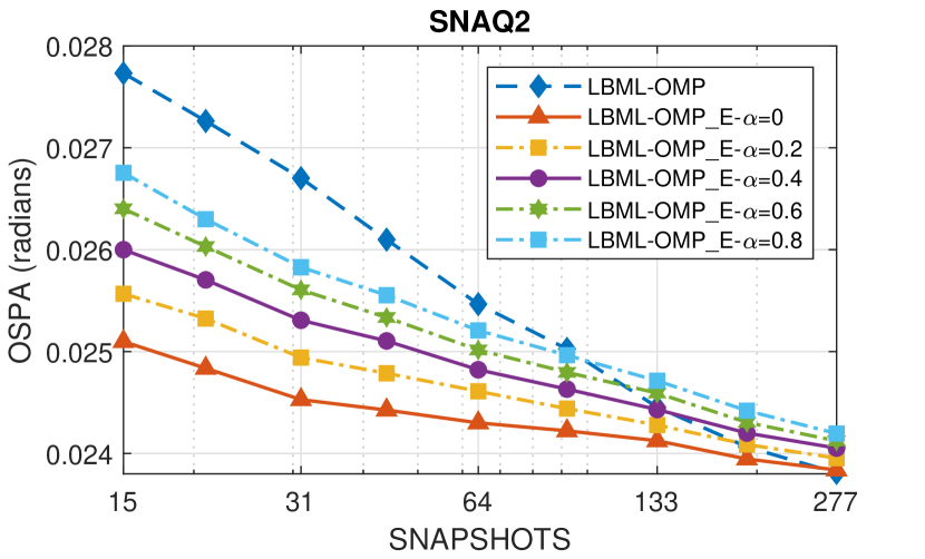
Figure 6: OSPA against snapshots with SNAQ2 geometry for LBML-OMP using DCTM and EDCTM (appended by “_E”) for $\alpha\in\left\{0,0.2,0.4,0.6,0.8\right\}$. SNR$=10$ dB.

VI Conclusion

We have developed an enhanced coarray estimation model termed EDCTM along with the LBML-OMP algorithm, which exploits the correlation-maximization in OMP and the asymptotic ML DOA estimator. The results show that the proposed approaches outperform existing techniques for DOA estimation and highlight errors introduced by the traditional difference coarray transformation in finite-sample scenarios.

References

- [1] H. L. Van Trees, Optimum Array Processing: Part IV of Detection, Estimation, and Modulation Theory. New York, USA: John Wiley & Sons, Inc., mar 2002.
- [2] R. de Lamare and R. Sampaio-Neto, “Adaptive reduced-rank mmse filtering with interpolated fir filters and adaptive interpolators,” IEEE Signal Processing Letters, vol. 12, no. 3, pp. 177–180, 2005.
- [3] R. C. de Lamare and R. Sampaio-Neto, “Reduced-rank adaptive filtering based on joint iterative optimization of adaptive filters,” IEEE Signal Processing Letters, vol. 14, no. 12, pp. 980–983, 2007.
- [4] L. Wang, “Constrained adaptive filtering algorithms based on conjugate gradient techniques for beamforming,” IET Signal Processing, vol. 4, pp. 686–697(11), December 2010. [Online]. Available: https://digital-library.theiet.org/content/journals/10.1049/iet-spr.2009.0243
- [5] R. C. de Lamare and R. Sampaio-Neto, “Adaptive reduced-rank processing based on joint and iterative interpolation, decimation, and filtering,” IEEE Transactions on Signal Processing, vol. 57, no. 7, pp. 2503–2514, 2009.
- [6] M. Yukawa, R. C. de Lamare, and R. Sampaio-Neto, “Efficient acoustic echo cancellation with reduced-rank adaptive filtering based on selective decimation and adaptive interpolation,” IEEE Transactions on Audio, Speech, and Language Processing, vol. 16, no. 4, pp. 696–710, 2008.
- [7] R. Fa, R. C. de Lamare, and L. Wang, “Reduced-rank stap schemes for airborne radar based on switched joint interpolation, decimation and filtering algorithm,” IEEE Transactions on Signal Processing, vol. 58, no. 8, pp. 4182–4194, 2010.
- [8] R. C. de Lamare and R. Sampaio-Neto, “Reduced-rank space–time adaptive interference suppression with joint iterative least squares algorithms for spread-spectrum systems,” IEEE Transactions on Vehicular Technology, vol. 59, no. 3, pp. 1217–1228, 2010.
- [9] ——, “Adaptive reduced-rank equalization algorithms based on alternating optimization design techniques for mimo systems,” IEEE Transactions on Vehicular Technology, vol. 60, no. 6, pp. 2482–2494, 2011.
- [10] R. de Lamare, Electronics Letters, vol. 44, pp. 565–567(2), April 2008. [Online]. Available: https://digital-library.theiet.org/content/journals/10.1049/el_20080627
- [11] R. de Lamare, L. Wang, and R. Fa, “Adaptive reduced-rank lcmv beamforming algorithms based on joint iterative optimization of filters: Design and analysis,” Signal Processing, vol. 90, no. 2, pp. 640–652, 2010. [Online]. Available: https://www.sciencedirect.com/science/article/pii/S0165168409003466
- [12] R. Fa, R. C. de Lamare, and L. Wang, “Reduced-rank stap schemes for airborne radar based on switched joint interpolation, decimation and filtering algorithm,” IEEE Transactions on Signal Processing, vol. 58, no. 8, pp. 4182–4194, 2010.
- [13] S. Xu, R. C. de Lamare, and H. Vincent Poor, “Distributed low-rank adaptive estimation algorithms based on alternating optimization,” Signal Processing, vol. 144, pp. 41–51, 2018. [Online]. Available: https://www.sciencedirect.com/science/article/pii/S0165168417303456
- [14] R. C. de Lamare, M. Haardt, and R. Sampaio-Neto, “Blind adaptive constrained reduced-rank parameter estimation based on constant modulus design for cdma interference suppression,” IEEE Transactions on Signal Processing, vol. 56, no. 6, pp. 2470–2482, 2008.
- [15] R. C. de Lamare, R. Sampaio-Neto, and M. Haardt, “Blind adaptive constrained constant-modulus reduced-rank interference suppression algorithms based on interpolation and switched decimation,” IEEE Transactions on Signal Processing, vol. 59, no. 2, pp. 681–695, 2011.
- [16] S. D. Somasundaram, N. H. Parsons, P. Li, and R. C. de Lamare, “Reduced-dimension robust capon beamforming using krylov-subspace techniques,” IEEE Transactions on Aerospace and Electronic Systems, vol. 51, no. 1, pp. 270–289, 2015.
- [17] H. Ruan and R. C. de Lamare, “Robust adaptive beamforming using a low-complexity shrinkage-based mismatch estimation algorithm,” IEEE Signal Processing Letters, vol. 21, no. 1, pp. 60–64, 2014.
- [18] H. Ruan, “Low-complexity robust adaptive beamforming algorithms exploiting shrinkage for mismatch estimation,” IET Signal Processing, vol. 10, pp. 429–438(9), July 2016. [Online]. Available: https://digital-library.theiet.org/content/journals/10.1049/iet-spr.2014.0331
- [19] S. Xu, R. C. de Lamare, and H. V. Poor, “Distributed compressed estimation based on compressive sensing,” IEEE Signal Processing Letters, vol. 22, no. 9, pp. 1311–1315, 2015.
- [20] H. Ruan and R. C. de Lamare, “Robust adaptive beamforming based on low-rank and cross-correlation techniques,” IEEE Transactions on Signal Processing, vol. 64, no. 15, pp. 3919–3932, 2016.
- [21] ——, “Distributed robust beamforming based on low-rank and cross-correlation techniques: Design and analysis,” IEEE Transactions on Signal Processing, vol. 67, no. 24, pp. 6411–6423, 2019.
- [22] Z. Yang, R. C. de Lamare, and X. Li, “ -regularized stap algorithms with a generalized sidelobe canceler architecture for airborne radar,” IEEE Transactions on Signal Processing, vol. 60, no. 2, pp. 674–686, 2012.
- [23] N. Song, W. U. Alokozai, R. C. de Lamare, and M. Haardt, “Adaptive widely linear reduced-rank beamforming based on joint iterative optimization,” IEEE Signal Processing Letters, vol. 21, no. 3, pp. 265–269, 2014.
- [24] X. Wu, Y. Cai, M. Zhao, R. C. de Lamare, and B. Champagne, “Adaptive widely linear constrained constant modulus reduced-rank beamforming,” IEEE Transactions on Aerospace and Electronic Systems, vol. 53, no. 1, pp. 477–492, 2017.
- [25] R. C. De Lamare and R. Sampaio-Neto, “Blind adaptive mimo receivers for space-time block-coded ds-cdma systems in multipath channels using the constant modulus criterion,” IEEE Transactions on Communications, vol. 58, no. 1, pp. 21–27, 2010.
- [26] T. Peng, R. C. de Lamare, and A. Schmeink, “Adaptive distributed space-time coding based on adjustable code matrices for cooperative mimo relaying systems,” IEEE Transactions on Communications, vol. 61, no. 7, pp. 2692–2703, 2013.
- [27] Y. Cai, R. C. de Lamare, B. Champagne, B. Qin, and M. Zhao, “Adaptive reduced-rank receive processing based on minimum symbol-error-rate criterion for large-scale multiple-antenna systems,” IEEE Transactions on Communications, vol. 63, no. 11, pp. 4185–4201, 2015.
- [28] C. T. Healy and R. C. de Lamare, “Design of ldpc codes based on multipath emd strategies for progressive edge growth,” IEEE Transactions on Communications, vol. 64, no. 8, pp. 3208–3219, 2016.
- [29] M. F. Kaloorazi and R. C. de Lamare, “Subspace-orbit randomized decomposition for low-rank matrix approximations,” IEEE Transactions on Signal Processing, vol. 66, no. 16, pp. 4409–4424, 2018.
- [30] ——, “Compressed randomized utv decompositions for low-rank matrix approximations,” IEEE Journal of Selected Topics in Signal Processing, vol. 12, no. 6, pp. 1155–1169, 2018.
- [31] L. Wang, R. C. de Lamare, and M. Haardt, “Direction finding algorithms based on joint iterative subspace optimization,” IEEE Transactions on Aerospace and Electronic Systems, vol. 50, no. 4, pp. 2541–2553, October 2014.
- [32] L. Qiu, Y. Cai, R. C. de Lamare, and M. Zhao, “Reduced-rank doa estimation algorithms based on alternating low-rank decomposition,” IEEE Signal Processing Letters, vol. 23, no. 5, pp. 565–569, May 2016.
- [33] Z. Shao, L. T. N. Landau, and R. C. de Lamare, “Dynamic oversampling for 1-bit adcs in large-scale multiple-antenna systems,” IEEE Transactions on Communications, pp. 1–1, 2021.
- [34] C. Stoeckle, J. Munir, A. Mezghani, and J. A. Nossek, “DoA Estimation Performance and Computational Complexity of Subspace- and Compressed Sensing-based Methods,” WSA 2015; 19th International ITG Workshop on Smart Antennas; Proceedings of, pp. 1–6, 2015.
- [35] D. Malioutov, M. Çetin, and A. S. Willsky, “A sparse signal reconstruction perspective for source localization with sensor arrays,” IEEE Transactions on Signal Processing, vol. 53, no. 8, pp. 3010–3022, 2005.
- [36] W. K. Ma, T. H. Hsieh, and C. Y. Chi, “DOA estimation of quasi-stationary signals via Khatri-Rao subspace,” ICASSP, IEEE International Conference on Acoustics, Speech and Signal Processing - Proceedings, pp. 2165–2168, 2009.
- [37] P. Pal and P. P. Vaidyanathan, “A novel array structure for directions-of-arrival estimation with increased degrees of freedom,” in 2010 IEEE International Conference on Acoustics, Speech and Signal Processing, 2010, pp. 2606–2609.
- [38] P. Pal and P. P. Vaidyanathan, “Nested arrays: A novel approach to array processing with enhanced degrees of freedom,” IEEE Transactions on Signal Processing, vol. 58, no. 8, pp. 4167–4181, 2010.
- [39] Y. D. Zhang, M. G. Amin, and B. Himed, “Sparsity-based DOA estimation using co-prime arrays,” ICASSP, IEEE International Conference on Acoustics, Speech and Signal Processing - Proceedings, pp. 3967–3971, 2013.
- [40] Y. Pati, R. Rezaiifar, and P. Krishnaprasad, “Orthogonal matching pursuit: recursive function approximation with applications to wavelet decomposition,” in Proceedings of 27th Asilomar Conference on Signals, Systems and Computers, vol. 1. IEEE Comput. Soc. Press, 1993, pp. 40–44.
- [41] T. Blumensath and M. E. Davies, “Iterative hard thresholding for compressed sensing,” Applied and Computational Harmonic Analysis, vol. 27, no. 3, pp. 265–274, 2009.
- [42] D. Needell and J. Tropp, “CoSaMP: Iterative signal recovery from incomplete and inaccurate samples,” Applied and Computational Harmonic Analysis, vol. 26, no. 3, pp. 301–321, may 2009.
- [43] P. Gerstoft, C. F. Mecklenbrauker, A. Xenaki, and S. Nannuru, “Multisnapshot Sparse Bayesian Learning for DOA,” IEEE Signal Processing Letters, vol. 23, no. 10, pp. 1469–1473, oct 2016. [Online]. Available: http://ieeexplore.ieee.org/document/7536146/
- [44] M. Dehghani and K. Aghababaiyan, “FOMP algorithm for Direction of Arrival estimation,” Physical Communication, vol. 26, pp. 170–174, feb 2018. [Online]. Available: https://doi.org/10.1016/j.phycom.2017.12.012https://linkinghub.elsevier.com/retrieve/pii/S1874490717303932
- [45] A. Jaffer, “Maximum likelihood direction finding of stochastic sources: a separable solution,” in ICASSP-88., International Conference on Acoustics, Speech, and Signal Processing. IEEE, 1988, pp. 2893–2896.
- [46] Z.-M. Liu, Z.-T. Huang, Y.-Y. Zhou, and J. Liu, “Direction-of-Arrival Estimation of Noncircular Signals via Sparse Representation,” IEEE Transactions on Aerospace and Electronic Systems, vol. 48, no. 3, pp. 2690–2698, jul 2012.
- [47] C.-L. Liu and P. P. Vaidyanathan, “Super Nested Arrays: Linear Sparse Arrays With Reduced Mutual Coupling—Part I: Fundamentals,” IEEE Transactions on Signal Processing, vol. 64, no. 15, pp. 3997–4012, aug 2016.
- [48] B. Carlson, “Covariance matrix estimation errors and diagonal loading in adaptive arrays,” IEEE Transactions on Aerospace and Electronic Systems, vol. 24, no. 4, pp. 397–401, jul 1988.
- [49] W.-k. Ma, T.-h. Hsieh, and C.-y. Chi, “DOA Estimation of Quasi-Stationary Signals With Less Sensors Than Sources and Unknown Spatial Noise Covariance: A Khatri–Rao Subspace Approach,” IEEE Transactions on Signal Processing, vol. 58, no. 4, pp. 2168–2180, apr 2010.
- [50] N. R. Goodman, “Statistical Analysis Based on a Certain Multivariate Complex Gaussian Distribution (An Introduction),” The Annals of Mathematical Statistics, vol. 34, no. 1, pp. 152–177, mar 1963. [Online]. Available: http://projecteuclid.org/euclid.aoms/1177704250
- [51] D. Maiwald and D. Kraus, “Calculation of moments of complex Wishart and complex inverse Wishart distributed matrices,” IEE Proceedings - Radar, Sonar and Navigation, vol. 147, no. 4, p. 162, 2000.
- [52] A. Koochakzadeh and P. Pal, “Exact localization of correlated sources using 2D harmonics retrieval,” in 2016 50th Asilomar Conference on Signals, Systems and Computers. IEEE, nov 2016, pp. 1503–1507. [Online]. Available: http://ieeexplore.ieee.org/document/7869628/
- [53] S. Foucart and H. Rauhut, A Mathematical Introduction to Compressive Sensing, ser. Applied and Numerical Harmonic Analysis. New York, NY: Springer, feb 2013.
- [54] K. Aghababaiyan, V. Shah-Mansouri, and B. Maham, “High-Precision OMP-Based Direction of Arrival Estimation Scheme for Hybrid Non-Uniform Array,” IEEE Communications Letters, vol. 24, no. 2, pp. 354–357, feb 2020. [Online]. Available: https://ieeexplore.ieee.org/document/8895771/
- [55] W. Dai and O. Milenkovic, “Subspace pursuit for compressive sensing signal reconstruction,” IEEE Transactions on Information Theory, vol. 55, no. 5, pp. 2230–2249, 2009.
- [56] Z. Ye, J. Dai, X. Xu, and X. Wu, “DOA estimation for uniform linear array with mutual coupling,” IEEE Transactions on Aerospace and Electronic Systems, vol. 45, no. 1, pp. 280–288, 2009.
- [57] A. Moffet, “Minimum-redundancy linear arrays,” IEEE Transactions on Antennas and Propagation, vol. 16, no. 2, pp. 172–175, mar 1968.
- [58] E. Vertatschitsch and S. Haykin, “Nonredundant arrays,” Proceedings of the IEEE, vol. 74, no. 1, pp. 217–217, 1986.
- [59] Z. Shi, C. Zhou, Y. Gu, N. A. Goodman, and F. Qu, “Source Estimation Using Coprime Array: A Sparse Reconstruction Perspective,” IEEE Sensors Journal, vol. 17, no. 3, pp. 755–765, feb 2017.