[table]capposition=top
Modelling Point Referenced Spatial Count Data: A Poisson Process Approach
Abstract
Random fields are useful mathematical tools for representing natural phenomena with complex dependence structures in space and/or time. In particular, the Gaussian random field is commonly used due to its attractive properties and mathematical tractability. However, this assumption seems to be restrictive when dealing with counting data. To deal with this situation, we propose a random field with a Poisson marginal distribution considering a sequence of independent copies of a random field with an exponential marginal distribution as “inter-arrival times” in the counting renewal processes framework. Our proposal can be viewed as a spatial generalization of the Poisson counting process.
Unlike the classical hierarchical Poisson Log-Gaussian model, our proposal generates a (non)-stationary random field that is mean square continuous and with Poisson marginal distributions. For the proposed Poisson spatial random field, analytic expressions for the covariance function and the bivariate distribution are provided. In an extensive simulation study, we investigate the weighted pairwise likelihood as a method for estimating the Poisson random field parameters.
Finally, the effectiveness of our methodology is illustrated by an analysis of reindeer pellet-group survey data, where a zero-inflated version of the proposed model is compared with zero-inflated Poisson Log-Gaussian and Poisson Gaussian copula models. Supplementary materials for this article, including technical proofs and R code for reproducing the work, are available as an online supplement.
Keywords: Gaussian random field; Gaussian copula; Pairwise likelihood function; Poisson distribution; Renewal process
1 Introduction
The faecal pellet count technique is one of the most popular tool for estimating an animal species’ abundance. Specifically, this technique uses the number of observed droppings combined with their decay time and the target animal species’ defecation rate. With these ingredients, it is possible to obtain an accurate density estimation of an animal population. This method was proposed by Bennett et al. (1940) and has been improved by several authors (see for example Etten and Bennett, 1965; Mayle et al., 1999; Krebs et al., 2001, among others).
The study motivating our research is a reindeer pellet-group survey conducted in the northern forest area of Sweden and previously analysed by Lee et al. (2016). The objective of this survey was to assess the impact of newly established wind farms on reindeer habitat selection. This choice is crucial for the reindeer since it involves trade‐offs between fulfilling necessities for feeding, mating, parental care, and risk mitigation of predation (Sivertsen et al., 2016).
Survey data was collected over the years 2009–2010 and presented a large number of zero counts. This situation is frequent when spatial species count data are collected since the survey is conducted using a point transect design (Buckland et al., 2001). This design considers a set of plots as systematically spaced plots along lines (transects) located throughout the survey region, where should be at least 20 for obtaining robust estimates of the abundance. The study area was 250 km2, the distance between each transect was 300 m. On each transect, the distance between each plot was 100 m. The size of each plot was 15 m2 with a radius of 2.18 m.
From a modelling viewpoint, the analysis of the reindeer pellet-group data requires the development of statistical models for geo-referenced count data that take into account both spatial dependence and the excessive number of zeros. Random fields or stochastic processes are useful models when dealing with geo-referenced spatial or spatio-temporal data (Stein, 1999; Cressie and Wikle, 2011; Banerjee et al., 2014). In particular, the Gaussian random field is widely used due to its attractive properties and mathematical tractability (Gelfand and Schliep, 2016). Gaussianity is clearly a restrictive assumption when dealing with counting data. However, many models of current use for spatial count data employ Gaussian random fields as building blocks.
The first example is the hierarchical model approach proposed by Diggle et al. (1998), which can be viewed as a generalized linear mixed model (Diggle and Ribeiro, 2007; Diggle and Giorgi, 2019). Under this framework, non-Gaussian models for spatial data can be specified using a link function and a latent Gaussian random field through a conditionally independence assumption. In particular, the Poisson Log-Gaussian random field (Poisson LG hereafter) has been widely applied for modelling count spatial data (see for instance Christensen and Waagepetersen, 2002; Guillot et al., 2009; De Oliveira, 2013, for interesting applications and in-depth study of its properties). Similar models, that can be defined hierarchically in terms of the specification of the first two moments and a correlation function have been proposed in Monestiez et al. (2006) and De Oliveira (2014).
It is important to stress that the conditional independence assumption underlying these kind of models leads to (a) random fields with marginal distributions that are not Poisson and (b) random fields with a “forced” nugget effects that implies no mean square continuity.
 |
 |
| (a) | (b) |
 |
 |
| (c) | (d) |
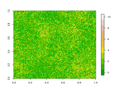
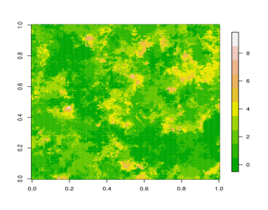
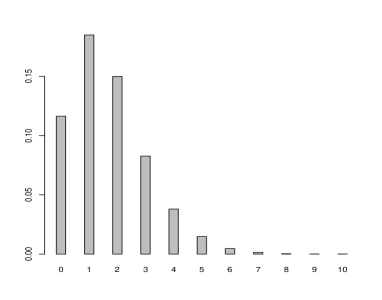
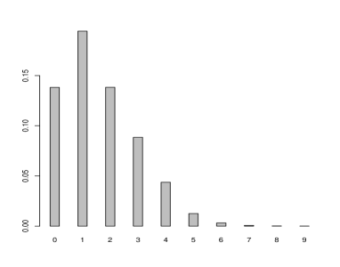
To illustrate this situation, Figure 1 (a) shows a realization on the unit square of a Poisson LG random field, , where is the standard Gaussian random field with isotropic correlation belonging to the Generalized Wendland family (Bevilacqua et al., 2019), , , is the spatial distance and denotes the positive part. In this case, the mean of the Poisson LG field is given by . The associated histogram is shown in panel (d).
Additionally, Figure 1 (b) shows a realization and the associated histogram of our proposed random field (see Equation (2)), with the same mean and underlying correlation function of the Poisson LG model. A quick analysis of both figures reveals a “whitening” effect on the Poisson LG random field’s paths because of the “forced” discontinuity at the origin of the correlation function for the Poisson LG (see Section 3.1). This potential problem, which has also been highlighted by De Oliveira (2013), indicates that the Poisson LG random field may impose severe restrictions on the correlation structure and may be inadequate to model spatial count data specially consisting of small counts.
The second example is the Poisson spatial model obtained using Gaussian copula (Kazianka and Pilz, 2010; Masarotto and Varin, 2012; Joe, 2014), which is referred to as the Poisson GC random field hereafter. This approach has some potential benefits with respect to the hierarchical models (see Han and De Oliveira, 2016, for a comparison between these two approaches). For example, the resulting random field has Poisson marginals and can or cannot be mean square continuous depending on whether the latent Gaussian random field is mean square continuous or not. In addition to some some criticisms concerning the lack of uniqueness of the copula when applied to discrete data (Genest and Nešlehová, 2007; Trivedi and Zimmer, 2017), this approach has no clarity regarding what underlying physical mechanism is generating the data, making it less interesting from an interpretability perspective.
Our proposal tries to solve the drawbacks of the Poisson LG and of the Poisson GC approaches by specifying a new class of spatial counting random fields based on the Poisson counting process (Cox, 1962; Mainardi et al., 2007; Ross, 2008) applied to the spatial setting. Specifically, we first consider a random field with exponential marginal distributions obtained as a rescaled sum of two independent copies of an underlying standard Gaussian random field. Then, by considering independent copies of the exponential random field as inter-arrival times in the counting renewal processes framework, we obtain a (non-)stationary random field with Poisson marginal distributions. By construction, for each spatial location, the proposed model is a Poisson counting process i.e. it represents the random number of events occurring in an arbitrary interval of time when the time between the occurrence of two events is exponentially distributed. More importantly, given two location sites, the associated Poisson counting processes are spatially correlated. For this reason, the proposed model can be viewed as a spatial generalization of the Poisson process.
For the novel Poisson random field, we provide the covariance function and analytic expressions for the bivariate distribution in terms of the regularized incomplete Gamma and confluent hypergeometric functions (Gradshteyn and Ryzhik, 2007). It follows that the dependence of the proposed Poisson random field is indexed by the correlation function of the underlying Gaussian random field and by the mean parameter. It is important to stress that our theoretical results are inspired by the two-dimensional renewal theory described in Hunter (1974).
The Poisson random field estimation is performed with the weighted pairwise likelihood (wpl) method (Lindsay, 1988; Varin et al., 2011; Bevilacqua and Gaetan, 2015) exploiting the results obtained from the bivariate distribution. In particular, in an extensive simulation study, we explore the efficiency of the wpl method when estimating the parameters of the proposed Poisson random field. We also explore the statistical efficiency of a Gaussian misspecified version of the wpl method (Gouriéroux et al., 2017; Bevilacqua et al., 2021), which is also called Gaussian quasi-likelihood in some literature (Masuda, 2013). The findings show that the misspecified wpl leads to a less efficient estimator, in particular for low counts. However, the method has some computational benefits. In addition, we compare the performance of the optimal linear predictor under the proposed model with the optimal predictors obtained using the Poisson GC and Poisson LG models.
Finally, in the real data application, we consider a zero-inflated version of the proposed Poisson random field to deal with excess zeros in the reindeer pellet-group counts data, using the zero-inflated Poisson LG and Poisson GC models as benchmarks. The methods proposed in this paper are implemented in the R (R Core Team, 2020) package GeoModels (Bevilacqua et al., 2022) and R code for reproducing the work is available as an online supplement.
The remainder of the paper is organized as follows. In Section 2, we provide some basic notation and describe the exponential random field. Section 3 introduces our proposal by presenting a new class of counting random fields under the general renewal counting framework, focusing on the Poisson random field. A study of the associated correlation function and bivariate distribution is presented and, in addition, a zero-inflated extension of the proposed model is introduced. In Section 4, the wpl method for obtaining the wpl estimates and the optimal linear prediction is discussed. Section 5 provides an in-depth simulation study to investigate the performance of the Poisson random field in spatial and spatio-temporal settings. In Section 6, the faecal pellet-group counts dataset previously described is re-analysed. Section 7 closes the paper with a discussion of our main findings and future research directions.
2 A random field with exponential marginal distributions
To make the paper self-contained, we start by introducing some notation in this Section. For the rest of the paper, given a second order real-valued random field , we denote by and the marginal probability density function (pdf) and cumulative distribution function (cdf) of , respectively. Moreover, for any set of distinct points , and , we denote the correlation function by . In the stationary case, the adopted notation is , where is the lag separation vector. Finally, denotes the pdf of the bivariate random vector , . If the random field is a discrete-valued random field, then and , will denote the marginal and bivariate discrete probability functions, respectively.
Let be a zero mean and unit variance weakly stationary Gaussian random field with correlation function . Henceforth, we call the Gaussian underlying random field, and with some abuse of notation, we set , denoting this as the underlying correlation function. Let be two independent copies of and let us define the random field as follows:
| (1) |
where is a non-random function. is a stationary random field with a marginal exponential distribution, with parameter denoted by with , , and it can be easily observed that .
The associated multivariate exponential density was discussed earlier by Krishnamoorthy and Parthasarathy (1951), and since then, its properties have been studied by several authors (Krishnaiah and Rao, 1961; Royen, 2004). However, likelihood-based methods for exponential random fields can be troublesome since the analytical expressions of the multivariate density can be derived only in some specific cases. For example, when and the underlying correlation function is exponential, the multivariate pdf is given by (Bevilacqua et al., 2020):
with , , and being the modified Bessel function of the first kind of order . Regardless of the dimension of the space and the type of correlation function, the bivariate exponential pdf is given by (Kibble, 1941; Vere-Jones, 1997):
The exponential random field will be further used to define a new random field with Poisson marginal distributions.
3 Spatial Poisson random fields
Our proposal relies on considering an infinite sequence of independent copies , of , a positive continuous random field. We define a new class of counting random fields, , , as follows:
| (2) |
where is the -fold convolution of and represents the random total number of events that have occurred up to time at location site . In our approach, we are assuming that the location sites share a common time . This assumption is justified since the observation window is fixed for each location site in the pellet group count application.
The proposed model can be viewed as a spatial generalization of the renewal counting processes (Cox, 1962; Mainardi et al., 2007), where we consider independent copies of a positive random field as inter-arrival times or waiting times, instead of an independent and identically distributed sequence of positive random variables.
For each , and using the classical results from the renewal counting processes theory, the marginal discrete probability function of is given by:
| (3) |
In addition, the marginal mean (the so-called renewal function) and the variance of are given, respectively, by:
Different elections of the positive random field lead to counting random fields with specific marginal distributions.
In this paper, we assume that the “spatial inter-arrival times” are exponentially distributed i.e. we assume , where is the positive random field defined in (1), with marginal distribution and cdf given by , . In this case, with is an Erlang distribution, with cdf given by:
and from (3), we can obtain the marginal distribution of as:
| (4) |
with .
By construction, for each , the proposed model is a Poisson counting process that is represents the random number of events that have occurred up to time , when the inter-arrival times are exponentially distributed. In addition, given two arbitrary location sites ,, the associated Poisson counting processes and are spatially correlated (see Section 3.1). Therefore, the proposed model can be viewed as a spatial generalization of the Poisson counting process. Hereafter and without loss of generality, is set to one, and is denoted as .
We will call a Poisson random field with underlying correlation because is marginally Poisson distributed and the dependence is indexed by a correlation function.
Note that, when the spatially varying mean (and variance) is not constant then is not stationary. A typical parametric specification for the mean is given by , where is a vector of covariates and even though other types of parametric and non-parametric specifications can be used.
It is important to note that although the proposed Poisson random field is defined on the -dimensional Euclidean space , the proposed method can be easily adapted to other spaces, such as the continuous space-time space, the spherical spaces or the discrete space. The key for this extension is the specification of a suitable underlying correlation function . For example, a correlation function defined on the space-time setting, i.e., (Gneiting, 2002) or on the sphere of arbitrary radius i.e., , (Gneiting, 2013; Porcu et al., 2016). In the case of lattice or areal data, a suitable precision matrix with an appropriate neighborhood structure should be specified for the underlying Gaussian Markov random field (Rue and Held, 2005).
3.1 Correlation function
The following result, which can be found in the pioneering work of Hunter (1974), provides the correlation function of the non-stationary Poisson random field with underlying correlation depending on the regularized lower incomplete Gamma function:
| (5) |
where is the lower incomplete Gamma function and is the Gamma function. Additionally, we define the function , which considers the product of two regularized lower incomplete Gamma function sharing a common parameter.
Theorem 1.
Let be a non-stationary Poisson random field with underlying correlation . Then,
with .
Proof.
For details, refer to Hunter (1974), Section 5.2 (pages 38-39).
The following result provides a closed form expression of the correlation function in terms of modified Bessel function for the stationary case.
Corollary 1.
In Theorem 1, when , the Poisson random field is weakly stationary with the correlation function given by:
| (6) |
where .
Proof.
See the online supplement.
Note that is well defined at the origin since implying that the Poisson random field is mean square continuous. Additionally, if , then and if then , i.e., it converges to the correlation function of an exponential random field.
Following the graphical example given in Figure 1, we now compare the correlation functions of the proposed Poisson random field with the correlation of the Poisson LG random field, which is defined hierarchically by first considering a LG random field defined as , where is a standard Gaussian random field with correlation , and then assuming with for . In this case, the first two moments of are given by and . Consequently, and following Aitchison and Ho (1989), the correlation function is given by if and
otherwise. This correlation is discontinuous at the origin and the nugget effect is given by:
It is apparent that the marginal mean has a strong impact on the nugget effect.
Figure 2 (a) depicts the correlation functions , , and , which correspond to Poisson LG random fields with mean and, , respectively. As underlying correlation model we assume . It can be appreciated that for large mean values, the nugget effect is negligible. However, for small mean values, the nugget effect can be huge, and it is the cause of the “whitening” effect observed in Figure 1 (a).
Figure 2 (b) depicts the correlation function of the proposed Poisson random field using the same means and underlying correlation function of the Poisson LG random field. It can be appreciated that the correlation covers the entire range between 0 and 1, irrespective of the mean values.
Finally, Figure 2 (c) depicts the correlation function of the Poisson GC random field (Han and De Oliveira, 2016) defined as , where is the cdf of the standard Gaussian distribution and is the quantile function of the Poisson distribution and is a standard Gaussian random field with correlation . The correlation function in this case is given by
where is the pdf of the bivariate standard Gaussian distribution. It is apparent that the Poisson GC correlation is much stronger than , and it does not seem to be affected by the different mean values.
It is important to stress that the Poisson and the Poisson GC random fields that are not mean-square continuous can be obtained by introducing a nugget effect, i.e., a discontinuity at the origin of . This can be achieved by replacing the underlying correlation function with , where represents the underlying nugget effect.
 |
 |
 |
| (a) | (b) | (c) |
3.2 Bivariate distribution
In this section, we provide the bivariate distribution of the Poisson random field. This distribution can be written in terms of an infinite series depending on the regularized lower incomplete Gamma function defined in (5) and the regularized hypergeometric confluent function (Gradshteyn and Ryzhik, 2007), defined as:
where is the standard hypergeometric confluent function.
For the sake of simplicity, we analyze the following cases separately: (a) , (b) and , (c) , and (d) , . Moreover, we set , , and for notational convenience. We additionally define the function as follows:
Theorem 2.
Let be a Poisson random field with underlying correlation and mean . Then the bivariate distribution is given by:
(a) Case :
(b) Cases and :
respectively, where
(c) Case :
(d) Cases with , and with ,
respectively, where
Proof.
See the online supplement.
The evaluation of the bivariate distribution can be troublesome at first sight. However, it can be performed by truncating the series and considering that efficient numerical computation of the regularized lower incomplete gamma and hypergeometric confluent functions can be found in different libraries, such as the GNU scientific library (Gough, 2009) and the most important statistical softwares including R, Matlab, and Python. In particular, the R package Geomodels (Bevilacqua et al., 2022) uses the Python implementations in the SciPy library (Virtanen et al., 2020).
The bivariate distribution can be written as the product of two independent Poisson distributions when . This result, provided by Hunter (1974) in Theorem 3.6, establishes that the independence of two renewal counting processes is equivalent to a zero correlation between them. As outlined in Section 3.1, implies . Consequently, pairwise independence at the level of the underlying Gaussian random field implies pairwise independence for the Poisson random field.
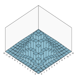
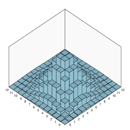
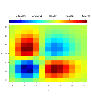
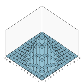
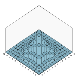
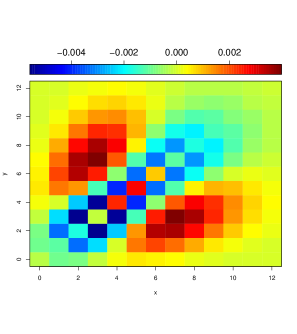
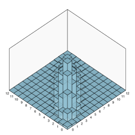
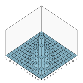
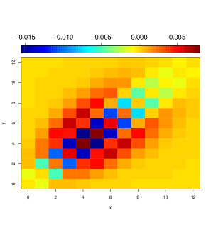
We now compare the type of bivariate dependence induced by the proposed model and the GC one when . Figure (3) (from left to right) presents the bivariate GC distribution, the bivariate Poisson distribution in Theorem 2 and a coloured image representing the differences between them. Note that a positive value of the difference implies that probabilities associated with bivariate distribution in Theorem 2 are greater than the probabilities of the bivariate GC one. Only the probabilities for are considered in the plots. The first, second and third row consider increasing levels of underlying correlations . It can be appreciated that the larger the correlation, the more significant is the difference between the proposed and Gaussian copula bivariate distributions. In addition, there is a pattern in which the probabilities of the GC bivariate distribution tend to be larger along the diagonal, i.e., the blue scale color is predominant along the diagonal. This is not surprising since the Poisson GC bivariate distribution inherits the type of dependence of the bivariate Gaussian distribution.
 |
 |
 |
|
 |
 |
|
 |
 |
| (a) | (b) | (c) |
3.3 A zero-inflated extension
In this Section we provide an extension of the proposed model for spatial data which exhibit an excessive number of zeros. Specifically, let , a Bernoulli random field such that , where is a Gaussian random field with , unit variance and correlation function . The marginal probability of having a zero is then given by:
where is the univariate standard Gaussian cdf. Let be a Poisson random field with and underlying correlation . Assuming and are independent, the proposed Poisson zero-inflated model is then given by a random field defined as:
| (7) |
with marginal distribution given by:
| (8) |
and with and . Note that the zero-inflated Poisson random field is overdispersed and when then the Poisson random field is obtained as special case. For the sake of completeness, we provide the bivariate distribution and the correlation function of the zero-inflated Poisson random field in Proposition 1 (see the online supplement).
4 Estimation and prediction
In this section, we start by describing the weighted pairwise likelihood (wpl) estimation method; then, we focus on the optimal linear prediction.
4.1 Weighted pairwise likelihood estimation
Composite likelihood is a general class of objective functions that combine low-dimensional terms based on the likelihood of marginal or conditional events to construct a pseudo likelihood Lindsay (1988); Varin et al. (2011). A particular case of the composite likelihood class is the pairwise likelihood (see for example Heagerty and Lele, 1998; Bevilacqua and Gaetan, 2015; Alegría et al., 2017; Bevilacqua et al., 2021, for application of pairwise likelihood in the spatial setting) that combines the bivariate distributions of all possible distinct pairs of observations. Let be a realization of the Poisson random field observed at distinct spatial locations , and let be the vector of unknown parameters where is the vector parameter associated with the underlying correlation model and the regression parameters. The pairwise likelihood function is defined as follows:
where is the bivariate density given in Theorem 2 and is a non-negative suitable weight. The choice of cut-off weights, namely,
| (9) |
for a positive value of , can be motivated by its simplicity and by observing that the dependence between distant observations is weak (Joe and Lee, 2009). Some guidelines on the choice of can be found in Bevilacqua et al. (2012); Bevilacqua and Gaetan (2015).
The maximum weighted pairwise likelihood (wpl) estimator is given by:
Under some mixing conditions of the Poisson random field, following Bevilacqua and Gaetan (2015), it can be shown that, when increasing domain asymptotic, is consistent and asymptotically Gaussian distributed, with the covariance matrix given by , i.e., the inverse of the Godambe information where and . The standard error estimation can be obtained from the square root diagonal elements of .
It is important to stress that the computation of the standard errors requires the evaluation of the matrices and . However, the evaluation of is computationally unfeasible for large datasets, and in this case, sub-sampling techniques can be used, as in Heagerty and Lele (1998) and Bevilacqua et al. (2012). A straightforward and more robust alternative is the parametric bootstrap estimation of (Bai et al., 2014).
Another critical issue related to large datasets is that computation of the wpl estimator can be computationally demanding due to the computational complexity associated with the bivariate Poisson distribution given in Theorem 2. An estimator that requires a smaller computational burden can be obtained under Gaussian misspecification (Masuda, 2013; Gouriéroux et al., 2017; Bevilacqua et al., 2021). This is a useful inferential tool when the likelihood function cannot be calculated for some reason, but the first two moments and the correlation are known.
In our case, we assume a non-stationary Gaussian random field with mean and variance equal to and correlation given in Theorem 1. Then the misspecified maximum requires the computation of the Gaussian bivariate distribution and the misspecified standard maximum likelihood estimation requires the computation of the Gaussian multivariate distribution. In both cases, evaluation of the Gamma incomplete function or the modified Bessel function (in the stationary case) is required to compute the covariance matrix. Table 1, in the online supplement, shows the computational cost of each estimation procedure through different scenarios for the stationary case, to demonstrate the computational gains of the Gaussian misspecified estimation with respect to the Poisson wpl estimation.
4.2 Optimal linear prediction
The Poisson random field’s optimal predictor concerning the mean squared error criterion requires the knowledge of the finite-dimensional distribution, which is not available for the Poisson random field. As in the estimation step, once again, the Gaussian misspecification allows to build the best linear unbiased predictor (BLUP) based on the correlation of the Poisson random field given in Theorem 1. Specifically, if the goal is the prediction of at given the vector of spatial observations observed at , then the optimal linear Gaussian prediction is given by:
| (10) |
where , and is the variance-covariance matrix ( the matrix Schur product). In practice, the mean and covariance matrix are not known and must be estimated. The associated mean squared error is:
Note that this kind of prediction does not guarantee the positivity and discreteness of the prediction. However, optimal linear prediction can generally be a useful approximation of the optimal predictor, as was shown, for example, in De Oliveira (2006) and recently in Bevilacqua et al. (2020). When is large the use of compactly supported correlation functions (Bevilacqua et al., 2019) can mitigate the computational burden associated with the optimal linear predictor since sparse matrix algorithms can be exploited to handle the inverse of the covariance matrix efficiently.
5 Simulation studies
In this section, we focus on two simulation studies. The first one analyses the performance of the wpl method when estimating the Poisson random field under the spatial and spatio-temporal settings. The second one analyses the Poisson optimal linear predictor’s performance, comparing our approach with the Poisson GC and Poisson LG models. This study is presented in the online supplement.
5.1 Performance of the wpl estimation
In this study, we consider realizations from a stationary spatial Poisson random field observed at , , . Specifically, we considered a regular grid with increments of size over the unit square . The grid points were perturbed, adding a uniform random value over to each coordinate. A perturbed grid allows us to obtain more stable estimates since different sets of small distances are available and very close location points are avoided. The simulation of the Poisson random field follows directly from the stochastic representation in (2), and it depends on the simulation of a sequence of independent copies of an exponential random field obtained by transforming independent copies of a standard Gaussian random field. These random fields were simulated using the Cholesky decomposition.
For the Poisson random field we, consider with , and an underlying isotropic correlation model with . As outlined in Section 3.2, the use of a compactly supported correlation function simplifies the computation of the bivariate Poisson distribution proposed in Theorem 2.
We study the performance of the Poisson wpl, the misspecified Gaussian wpl and the misspecified Gaussian maximum likelihood (ML) estimation methods. In the (misspecified) wpl estimation, we consider a cut-off weight function, as in (9), with .
| Poisson wpl | Gaussian wpl | Gaussian ML | ||||
|---|---|---|---|---|---|---|
| Bias | MSE | Bias | MSE | Bias | MSE | |
| -0.00251 | 0.00151 | -0.00348 | 0.00161 | -0.00366 | 0.00165 | |
| -0.00663 | 0.00113 | -0.00828 | 0.00208 | -0.00748 | 0.00203 | |
| -0.00113 | 0.00065 | -0.00147 | 0.00068 | -0.00161 | 0.00068 | |
| -0.00435 | 0.00098 | -0.00422 | 0.00149 | -0.00344 | 0.00145 | |
| 0.00052 | 0.00033 | 0.00031 | 0.00033 | 0.00014 | 0.00033 | |
| -0.00261 | 0.00096 | -0.00336 | 0.00120 | -0.00296 | 0.00115 | |
| -0.00026 | 0.00018 | -0.00039 | 0.00019 | -0.00037 | 0.00018 | |
| -0.00449 | 0.00094 | -0.00499 | 0.00099 | -0.00402 | 0.00095 | |
Table 1 shows the bias and mean squared error associated with and through the four scenarios and three estimation methods. As expected, the misspecified Gaussian ML performs slightly better than the misspecified Gaussian wpl. More importantly, it can be recognized that the Poisson wpl shows the best performance, particularly when estimating the spatial dependence parameter. This fact is more evident for low counts i.e., when is decreasing. However, when increasing the mean, the performances of the three methods of estimation tend to be considerably similar, in particular when the mean of the Poisson random field is .
To summarize, the Poisson wpl is the best method for estimating the Poisson random field when the mean is small (lower than 20 as a rule of thumb in our experiments). For large counts, the misspecified Gaussian wpl or ML methods show approximately the same performance as the Poisson wpl method.
We also study the proposed methods’ performance when estimating a non-stationary version of the Poisson random field. Under the previous simulation setting we changed the constant mean by considering a regression model, that is, with , and , where and are independent realizations from a uniform random variable. Table 2 shows the bias and MSE associated with , , and for the three methods of estimation, and Figure 1 of the online supplement plots the associated centred boxplots.
Additionally, in this case, the Poisson wpl method shows the best performance. We replicate the simulation by considering larger values of the regression parameters (the results are not reported here), which lead to larger counts, and the three methods of estimations show approximately the same performance as in the stationary case.
| Poisson wpl | Gaussian wpl | Gaussian ML | ||||
|---|---|---|---|---|---|---|
| Bias | MSE | Bias | MSE | Bias | MSE | |
| -0.00263 | 0.00419 | -0.00359 | 0.00445 | -0.00320 | 0.00428 | |
| 0.00189 | 0.00618 | 0.00148 | 0.00665 | 0.00046 | 0.00627 | |
| 0.00185 | 0.00608 | 0.00202 | 0.00661 | 0.00182 | 0.00621 | |
| -0.00148 | 0.00091 | -0.00030 | 0.00124 | 0.00096 | 0.00122 | |
Finally, we consider a simulation scheme under a spatio-temporal setting. Specifically, we consider simulations from a non-stationary space-time Poisson random field observed at , , spatial location sites, uniformly distributed within the unit square and , time points. We consider a regression model for the spatio-temporal mean , where , are independent realizations from a uniform random variable. We set , and as in the previous simulation scheme.
Additionally, as the underlying space-time correlation, we use a simple isotropic and temporal symmetric space-time Wendland separable model with and , where with . Finally, for the misspecified wpl estimation, we consider a cut-off weight function as in (9) extended to the space time case, with and .
The results concerning this simulation study are shown in Table 3, including the bias and MSE associated with , , and , for the three estimation methods. In addition, Figure 2 of the online supplement shows the associated box plots. As it can be observed, the Poisson wpl approach outperforms the misspecified Gaussian wpl and ML as expected for each parameter.
We want to highlight that we have replicated this simulation study by considering higher regression parameters’ values, leading to larger counts (for space reasons, these results are not reported here). In that case, all of the estimation methods showed similar behaviours as in the purely spatial case.
| Poisson wpl | Gaussian wpl | Gaussian ML | ||||
|---|---|---|---|---|---|---|
| Bias | MSE | Bias | MSE | Bias | MSE | |
| -0.00058 | 0.00166 | -0.00120 | 0.00180 | -0.00110 | 0.00167 | |
| -0.00079 | 0.00257 | -0.00056 | 0.00274 | -0.00102 | 0.00249 | |
| 0.00036 | 0.00284 | 0.00070 | 0.00302 | 0.00062 | 0.00267 | |
| -0.01057 | 0.00464 | -0.01323 | 0.00630 | -0.01343 | 0.00629 | |
| -0.00124 | 0.01846 | 0.00165 | 0.02534 | 0.00032 | 0.02415 | |
6 Application to the reindeer pellet-group survey in Sweden
As mentioned in the Introduction, the pellet-group survey is a technique that provides a general idea of species distribution over a specific geographic area. This technique is used, mainly, for (a) estimating the population density of several ungulate species such as deer (see for example Eberhardt and Van Etten, 1956; Freddy and Bowden, 1983; Mooty et al., 1984; Rowland et al., 1984; Marques et al., 2001, among many others) and (b) to study the impact of some covariates in the election of their habitat selection (see for example Skarin et al., 2015; Lee et al., 2016; Skarin and Alam, 2017).
Our analysis considers a reindeer pellet-group survey that was conducted on Storliden Mountain in the northern forest area of Sweden over the years 2009–2010. We focus in 2009 and specifically we consider pellet-group count data collected between June 3rd and 8th in 2009 (Lee et al., 2016). The main goal of the survey was to assess the impact of newly established wind farms on reindeer habitats.
In practice, we observe the total number of pellet-groups (a pellet-group is defined as a cluster of 20 or more pellets) at 357 location sites , . In this case, the mechanism generating the pellet-groups, for each location, can be assumed as a Poisson process, where the inter-arrival times between one pellet-group and another could be assumed to be exponentially distributed. Under this assumption, the proposed Poisson random field can be a useful tool to analyze the pellet-groups counts data.
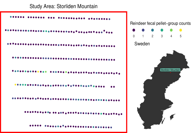
The dataset possesses two challenging features. The first one is that 73.67% of the counts are zeros since the animal might move as it defecates, and some plots present zero pellet-group counts (see Figure 4). The second one is that the empirical semi-variogram (see Figure 3 of the online supplement) exhibits both spatial correlation and a nugget effect.
To face this problem we consider the zero-inflated Poisson (ZIP) random field proposed in Section 3.3. and we compare it with the ZIP Gaussian copula (ZIP GC) using the R package gcKrig (Han and Oliveira, 2018). In addition, we consider the ZIP Log-Gaussian (ZIP LG) random field as implemented in the R package INLA (Rue et al., 2009; Lindgren et al., 2011; Martins et al., 2013) which exploits the integrated nested Laplace approximation, under a Bayesian framework, in the estimation step.
Since our application’s primary goal is to assess the impact of newly established wind farms on reindeer habitats, we are interested in relating the number of pellet-groups with covariates such as distance to power lines, slopes, or elevation of the field. Therefore, and following the results of Lee et al. (2016), we include three covariates: Northwest slopes (NS), Elevation (Eln) and Distance to power lines (DPL). In particular we specify as:
The parameterization for the marginal mean and variance is slightly different for the three models. Specifically, assuming that the probability of excess of zero counts does not depend on , the marginal mean and variance specifications are given by and for the proposed model, and for the GC model, and for the LG model.
Here, is specified as , with , as , with , and as , with , respectively, so , , can be interpreted as overdispersion parameters. It is important to remark that can not be compared between the different approaches, but , and can be compared.
We assume an underlying exponential correlation model with nugget effect for the ZIP GC and ZIP LG random fields. On the other hand for the proposed ZIP model we specify and that is two different underlying correlation models for and in (7) sharing a common exponential correlation model and different nugget effects .
We use maximum wpl estimation with in (9) for our ZIP random field. For the ZIP GC model, we perform maximum likelihood estimation as explained in Section 3 in the online supplement, and for ZIP LG model, we perform approximate Bayesian inference using the INLA approach (Rue et al., 2009).
Table 4 summarizes the results of the estimates, including their standard error for the three models. In the case of our ZIP random field, standard errors were computed by using parametric bootstrap (Efron and Tibshirani, 1986). For the Poisson LG model the reported estimates are the means of the posterior distributions with associated standard error.
Note that if is a positive value, then the counts of pellet-groups increase at larger distances from the power lines, i.e., there is a greater reindeer population far from the wind farms. The estimation of the regression parameters is quite similar for our ZIP and the ZIP GC models with lower standard error estimations for the GC model. On the other hand, our ZIP model shows the smallest standard error estimation of the spatial scale parameter . Finally, the estimates of , the excess of zero counts, which depend on , and for the ZIP, ZIP GC and ZIP LG random fields, are given by , , , respectively.
| ZIP | -23.423 | -0.534 | 0.005 | 2.594 | -0.048 | 339.132 | 0.868 | 0.624 | 0.797 | ||||
| (6.473) | (0.469) | (0.004) | (0.742) | (1.048) | (92.981) | (0.263) | (0.308) | ||||||
| ZIP GC | -19.096 | -0.465 | 0.003 | 2.060 | 0.912 | 298.926 | 0.714 | 0.800 | |||||
| (2.309) | (0.364) | (0.003) | (0.265) | (0.261) | (186.990) | (0.1285) | |||||||
| ZIP LG | -17.905 | -0.826 | 0.010 | 1.622 | 0.293 | 685.922 | 0.084 | 0.735 | 0.835 | ||||
| (9.514) | (0.388) | (0.005) | (1.177) | (0.098) | (354.614) | (0.022) | (0.396) |
The three models considered can also be used for prediction of the of pellet-group counts at specific not sampled location sites. In particular, this approach allows us to discover new areas for reindeer habitat employing the predicted number of pellet-groups, potentially providing information about the behavior of the reindeer population over the entire region. With this goal in mind, we want to assess the predictive performances of the three models. To do so, we randomly choose 80% of the spatial locations (i.e., location sites) for the parameter estimation and use the remaining 20% (i.e., location sites) for the predictions. We repeat this procedure times, recording the RMSE each time. Specifically, for each -th left-out sample , we compute
where is the optimal linear predictor for our ZIP random field (computed using the correlation given in Proposition 1 in the online supplement), the optimal predictor for the ZIP GC random field and the mean of the posterior predictive distribution for the ZIP LG random field. We report in Table 4, the empirical mean of the RMSE obtained for each left-out sample, i.e., . The ZIP and ZIP GC random fields’ clearly outperform the ZIP LG random field in terms of prediction performance. In particular the proposed ZIP random field provides the smallest .
Finally, as suggested by one Referee, we perform a simulation-based model assessment. Specifically, we simulated 10000 realizations under the three fitted models and counted the number of observations lying between the 95% probability intervals constructed with the simulated data. The results show that our ZIP proposed model and the ZIP GC are pretty similar, with 97.2% and 97.7% of the data lying in the 95% probability intervals, respectively. In the case of the ZIP LG, 96.9% of observations lie between the 95% probability interval.
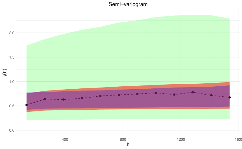
In addition, we compared the empirical semi-variogram of the data with the ones obtained from the simulations, and we found that our proposal (ZIP model) presents a small 95% probability interval compared to its competitors (a tight interval) (see Figure 5). This situation implies that our approach provides less uncertainty when estimating spatial dependence.
7 Concluding remarks
This paper has introduced a novel Poisson random field, i.e., a random field with Poisson marginal distributions, for regression and dependence analysis when addressing point-referenced count data defined on a spatial Euclidean space. However, the proposed methodology can be easily adapted to other types of data, such as space-time (Gneiting, 2013), areal (Rue and Held, 2005) or spherical data (Gneiting, 2013).
By construction, for each spatial location, the proposed model is a Poisson counting process, i.e., it represents the random total number of events occurring in an arbitrary interval of time when the inter-arrival times are exponentially distributed.
More importantly, given two arbitrary location sites, the associated Poisson counting processes are spatially correlated. For this reason, the proposed model can be viewed as a spatial generalization of the Poisson process.
The correlation between the Poisson counting processes is achieved by considering sequences of independent copies of a random field with an exponential marginal distribution as inter-arrival times in the counting renewal processes framework. The resulting (non-)stationary random field is marginally Poisson distributed and the dependence is indexed by a correlation function.
They key features of the proposed Poisson random field with respect to the Poisson Log-Gaussian random field are that its marginal distribution is Poisson distributed and it can be mean square continuous or not. The Poisson Gaussian copula approach shares these good features with our model. However, the generating mechanisms (i.e., the Poisson process), underlying our model makes it more appealing from interpretability viewpoint.
In our proposal, a possible limitation is that inference based on full likelihood cannot be performed due to the lack of amenable expressions of the associated multivariate distributions. Nevertheless, the simulations studies we conducted showed that our approach, based on a pairwise likelihood estimation seems to be an effective solution for estimating the unknown parameters involved in the Poisson random field. Another potential limitation is that the optimal predictor that minimizes the mean square prediction error is not available. However, our numerical experiments show that our solution based on optimal linear predictor performs very well when compared with the optimal predictors of the Poisson Gaussian copula and Poisson Log Gaussian models. Finally, the application of our model to the reindeer pellet-group survey data in Sweden shows that our approach can be easily adapted to handle spatial count data with an excessive number of zeros.
A well-known restriction of the Poisson distribution is equidispersion. Unfortunately, this situation is not always observed in real spatial data. The class of random fields proposed in (2) can be used to obtain random fields with flexible marginal models that consider over or under dispersion. In this case, a possible solution is to consider random fields with a more flexible marginal distribution than the exponential marginal distribution, such as the gamma or Weibull random fields (Bevilacqua et al., 2020). The resulting marginal counting models have been studied in Winkelmann (1995) and McShane et al. (2008). Another alternative for obtaining over dispersed random fields is considering scale mixtures of Poisson random fields. These topics are currently under study and will be included in a forthcoming paper.
Acknowledgements
The work of Diego Morales-Navarrete, Moreno Bevilacqua and Luis M. Castro was partially supported by ANID - Millennium Science Initiative Program - NCN17_059 from the Chilean government. Diego Morales-Navarrete also acknowledges support from the VRI-UC scholarship from the Pontificia Universidad Católica de Chile. Moreno Bevilacqua acknowledges financial support from Grant FONDECYT 1200068 and ANID/PIA/ANILLOS ACT210096, Chile and project Data Observatory Foundation DO210001 from the Chilean government. The work of Christian Caamaño was partially supported by grant FONDECYT 11220066 from the Chilean government and DIUBB 2120538 IF/R from University of Bío-Bío. Luis M. Castro acknowledges financial support from Grant FONDECYT 1220799 from the Chilean government.
References
- Aitchison and Ho (1989) Aitchison, J. and Ho, C. H. (1989). The multivariate Poisson-Log normal distribution. Biometrika 76, 643–653.
- Alegría et al. (2017) Alegría, A., Caro, S., Bevilacqua, M., Porcu, E., and Clarke, J. (2017). Estimating covariance functions of multivariate skew-gaussian random fields on the sphere. Spatial Statistics 22, 388 – 402.
- Bai et al. (2014) Bai, Y., Kang, J., and Song, P. (2014). Efficient pairwise composite likelihood estimation for spatial-clustered data. Biometrics 7, 661–670.
- Banerjee et al. (2014) Banerjee, S., Carlin, B. P., and Gelfand, A. E. (2014). Hierarchical Modeling and Analysis for Spatial Data. Chapman & Hall/CRC Press, Boca Raton: FL.
- Bennett et al. (1940) Bennett, L., English, P., and McCain, R. (1940). A study of deer populations by use of pellet-group counts. The Journal of Wildlife Management 4, 398–403.
- Bevilacqua et al. (2020) Bevilacqua, M., Caamaño-Carrillo, C., and Gaetan, C. (2020). On modelling positive continuous data with spatio-temporal dependence. Environmetrics 31, e2632.
- Bevilacqua et al. (2021) Bevilacqua, M., Caamaño-Carrillo, C., Arellano-Valle, R., and Morales-Oñate, V. (2021). Non-gaussian geostatistical modeling using (skew) t processes. Scandinavian Journal of Statistics 48, 212–245.
- Bevilacqua et al. (2019) Bevilacqua, M., Faouzi, T., Furrer, R., and Porcu, E. (2019). Estimation and prediction using generalized wendland functions under fixed domain asymptotics. The Annals of Statistics 47, 828–856.
- Bevilacqua and Gaetan (2015) Bevilacqua, M. and Gaetan, C. (2015). Comparing composite likelihood methods based on pairs for spatial Gaussian random fields. Statistics and Computing 25, 877–892.
- Bevilacqua et al. (2012) Bevilacqua, M., Gaetan, C., Mateu, J., and Porcu, E. (2012). Estimating space and space-time covariance functions for large data sets: a weighted composite likelihood approach. Journal of the American Statistical Association 107, 268–280.
- Bevilacqua et al. (2022) Bevilacqua, M., Morales-Oñate, V., and Caamaño-Carrillo, C. (2022). GeoModels: Procedures for Gaussian and Non Gaussian Geostatistical (Large) Data Analysis. R package version 1.0.2.
- Buckland et al. (2001) Buckland, S., Anderson, D. R., Burnham, K. P., Laake, J. L., Borchers, D. L., and Thomas, L. (2001). Introduction to Distance Sampling-estimating Abundance of Biological Populations. New York, NY., Oxford University Press.
- Christensen and Waagepetersen (2002) Christensen, O. and Waagepetersen (2002). Bayesian prediction of spatial count data using generalized linear mixed models. Biometrics 58, 280–286.
- Cox (1962) Cox, D. (1962). Renewal Theory. Methuen & Co, London.
- Cressie and Wikle (2011) Cressie, N. and Wikle, C. (2011). Statistics for Spatio-Temporal Data. Wiley Series in Probability and Statistics. Wiley.
- De Oliveira (2006) De Oliveira, V. (2006). On optimal point and block prediction in log-Gaussian random fields. Scandinavian Journal of Statistics 33, 523–540.
- De Oliveira (2013) De Oliveira, V. (2013). Hierarchical Poisson models for spatial count data. Journal of Multivariate Analysis 122, 93–408.
- De Oliveira (2014) De Oliveira, V. (2014). Poisson kriging: A closer investigation. Spatial Statistics 7, 1–20.
- Diggle and Giorgi (2019) Diggle, P. and Giorgi, E. (2019). Model-based Geostatistics for Global Public Health: Methods and Applications. Chapman & Hall/CRC Interdisciplinary Statistics. Chapman and Hall/CRC Press.
- Diggle et al. (1998) Diggle, P., Tawn, J., and Moyeed, R. (1998). Model-based geostatistics. Journal of the Royal Statistical Society: Series C (Applied Statistics) 47, 299–350.
- Diggle and Ribeiro (2007) Diggle, P. J. and Ribeiro, P. J. (2007). Model-based Geostatistics. Springer, New York.
- Eberhardt and Van Etten (1956) Eberhardt, L. and Van Etten, R. (1956). Evaluation of the pellet group count as a deer census method. Journal of Wildlife Management 20, 70–74.
- Efron and Tibshirani (1986) Efron, B. and Tibshirani, R. (1986). Bootstrap methods for standard errors, confidence intervals, and other measures of statistical accuracy. Statistical Science 1, 54–75.
- Etten and Bennett (1965) Etten, R. V. and Bennett, C. (1965). Some sources of error in using pellet-group counts for censusing deer. The Journal of Wildlife Management 29, 723–729.
- Freddy and Bowden (1983) Freddy, D. and Bowden, D. (1983). Sampling mule deer pellet-group densities in juniper-pinyon woodland. Journal of Wildlife Management 47, 476–485.
- Gelfand and Schliep (2016) Gelfand, A. E. and Schliep, E. M. (2016). Spatial statistics and Gaussian processes: A beautiful marriage. Spatial Statistics 18, 86–104. Spatial Statistics Avignon: Emerging Patterns.
- Genest and Nešlehová (2007) Genest, C. and Nešlehová, J. (2007). A primer of copulas for count data. ASTIN Bulletin 37, 475–515.
- Gneiting (2002) Gneiting, T. (2002). Stationary covariance functions for space-time data. Journal of the American Statistical Association 97, 590–600.
- Gneiting (2013) Gneiting, T. (2013). Strictly and non-strictly positive definite functions on spheres. Bernoulli 19, 1327–1349.
- Gough (2009) Gough, B. (2009). GNU Scientific Library Reference Manual. Network Theory Ltd.
- Gouriéroux et al. (2017) Gouriéroux, C., Monfort, A., and Renault, E. (2017). Consistent pseudo-maximum likelihood estimators. Annals of Economics and Statistics pages 187–218.
- Gradshteyn and Ryzhik (2007) Gradshteyn, I. and Ryzhik, I. (2007). Table of Integrals, Series, and Products. Academic Press, New York, 7 edition.
- Guillot et al. (2009) Guillot, G., Loren, N., and Rudemo, M. (2009). Spatial prediction of weed intensities from exact count data and image-based estimates. Journal of the Royal Statistical Society: Series C 58, 525–542.
- Han and De Oliveira (2016) Han, Z. and De Oliveira, V. (2016). On the correlation structure of Gaussian copula models for geostatistical count data. Australian & New Zealand Journal of Statistics 58, 47–69.
- Han and Oliveira (2018) Han, Z. and Oliveira, V. D. (2018). gckrig: An R package for the analysis of geostatistical count data using Gaussian copulas. Journal of Statistical Software 87, 1–32.
- Heagerty and Lele (1998) Heagerty, P. and Lele, S. (1998). A composite likelihood approach to binary spatial data. Journal of the American Statistical Association 93, 1099 –1111.
- Hunter (1974) Hunter, J. (1974). Renewal theory in two dimensions: basic results. Advances in Applied Probability 6, 376–391.
- Joe (2014) Joe, H. (2014). Dependence Modeling with Copulas. Chapman and Hall/CRC, Boca Raton, FL.
- Joe and Lee (2009) Joe, H. and Lee, Y. (2009). On weighting of bivariate margins in pairwise likelihood. Journal of Multivariate Analysis 100, 670–685.
- Kazianka and Pilz (2010) Kazianka, H. and Pilz, J. (2010). Copula-based geostatistical modeling of continuous and discrete data including covariates. Stochastic Environmental Research and Risk Assessment 24, 661–673.
- Kibble (1941) Kibble, W. F. (1941). A two-variate gamma type distribution. Sankhyā: The Indian Journal of Statistics 5, 137–150.
- Krebs et al. (2001) Krebs, C., Boonstra, R., Nams, V., M, M. O., Hodges, K., and Boutin, S. (2001). Estimating snowshoe hare population density from pellet plots: A further evaluation. Canadian Journal of Zoology 79, 1–4.
- Krishnaiah and Rao (1961) Krishnaiah, P. and Rao, M. (1961). Remarks on a multivariate gamma distribution. The American Mathematical Monthly 68(4), 342–346.
- Krishnamoorthy and Parthasarathy (1951) Krishnamoorthy, A. S. and Parthasarathy, M. (1951). A Multivariate Gamma-Type Distribution. The Annals of Mathematical Statistics 22(4), 549–557.
- Lee et al. (2016) Lee, Y., Moudud, A., Noh, M., Rönnegård, L., and Skarin, A. (2016). Spatial modeling of data with excessive zeros applied to reindeer pellet‐group counts. Ecology and Evolution 6, 7047–7056.
- Lindgren et al. (2011) Lindgren, F., Rue, H., , and Lindstrom, J. (2011). An explicit link between Gaussian fields and Gaussian Markov random fields: the stochastic partial differential equation approach. Journal of the Royal Statistical Society B 73, 423–498.
- Lindsay (1988) Lindsay, B. (1988). Composite likelihood methods. Contemporary Mathematics 80, 221–239.
- Mainardi et al. (2007) Mainardi, F., Gorenflo, R., and Vivoli, A. (2007). Beyond the Poisson renewal process: A tutorial survey. Journal of Computational and Applied Mathematics 205, 725 – 735. Special issue on evolutionary problems.
- Marques et al. (2001) Marques, F., Buckland, S., Goffin, D., Dixon, C., Borchers, D., Mayle, B., and Peace, A. (2001). Estimating deer abundance from line transect surveys of dung: sika deer in sourthern Scotland. Journal of Applied Ecology 38, 349–363.
- Martins et al. (2013) Martins, T. G., Simpson, D., Lindgren, F., and Rue, H. (2013). Bayesian computing with inla: new features. Computational Statistics and Data Analysis 67, 68–83.
- Masarotto and Varin (2012) Masarotto, G. and Varin, C. (2012). Gaussian copula marginal regression. Electronic Journal of Statistics 6, 1517–1549.
- Masuda (2013) Masuda, H. (2013). Convergence of Gaussian quasi-likelihood random fields for ergodic Lévy driven SDE observed at high frequency. The Annals of Statistics 41, 1593–1641.
- Mayle et al. (1999) Mayle, B., Peace, A., and Gill, R. (1999). How many deer? a field guide to estimating deer population size. Technical Report Forestry Commission Field book 18, Forestry Commission, Edinburgh.
- McShane et al. (2008) McShane, B., Adrian, M., Bradlow, E. T., and Fader, P. S. (2008). Count models based on weibull interarrival times. Journal of Business & Economic Statistics 26, 369–378.
- Monestiez et al. (2006) Monestiez, P., Dubroca, L., Bonnin, E., and Guinet, J.-P. D. C. (2006). Geostatistical modelling of spatial distribution of balaenoptera physalus in the northwestern mediterranean sea from sparse count data and heterogeneous. Ecological Modelling 193, 615–628.
- Mooty et al. (1984) Mooty, J., Karns, P., and Heisey, D. (1984). The relationship between white-tailed deer track counts and pellet-group surveys. Journal of Wildlife Management 48, 275–279.
- Porcu et al. (2016) Porcu, E., Bevilacqua, M., and Genton, M. G. (2016). Spatio-temporal covariance and cross-covariance functions of the great circle distance on a sphere. Journal of the American Statistical Association 111, 888–898.
- R Core Team (2020) R Core Team (2020). R: A Language and Environment for Statistical Computing. R Foundation for Statistical Computing, Vienna, Austria.
- Ross (2008) Ross, S. (2008). Stochastic Processes, 2nd. Ed. Wiley series in probability and mathematical statistics. Wiley India Pvt. Limited.
- Rowland et al. (1984) Rowland, M., White, G., and Karlen, E. (1984). Use of pellet-group plots to measure trends in deer and elk populations. Wildlife Society Bulletin 12, 147–155.
- Royen (2004) Royen, T. (2004). Multivariate Gamma distributions II. In Encyclopedia of Statistical Sciences, pages 419–425. New York: John Wiley & Sons.
- Rue and Held (2005) Rue, H. and Held, L. (2005). Gaussian Markov Random Fields: Theory and Applications. Chapman & Hall, London.
- Rue et al. (2009) Rue, H., Martino, S., and Chopin, N. (2009). Approximate Bayesian inference for latent Gaussian models using integrated nested Laplace approximations (with discussion). Journal of the Royal Statistical Society B 71, 319–392.
- Sivertsen et al. (2016) Sivertsen, T. R., Åhman, B., Steyaert, S. M. J. G., Rönnegård, L., Frank, J., Segerström, P., Støen, O.-G., and Skarin, A. (2016). Reindeer habitat selection under the risk of brown bear predation during calving season. Ecosphere 7, e01583.
- Skarin and Alam (2017) Skarin, A. and Alam, M. (2017). Reindeer habitat use in relation to two small wind farms, during preconstruction, construction, and operation. Ecology and Evolution 7, 3870–3882.
- Skarin et al. (2015) Skarin, A., Nelleman, C., Rönnegård, Sandström, P., and Lundqvist, H. (2015). Wind farm construction impacts reindeer migration and movement corridors. Landscape Ecology 30, 1527–1540.
- Stein (1999) Stein, M. (1999). Interpolation of Spatial Data. Some Theory of Kriging. Springer-Verlag, New York.
- Trivedi and Zimmer (2017) Trivedi, P. and Zimmer, D. (2017). A note on identification of bivariate copulas for discrete count data. Econometrics 5(1), 1–11.
- Varin et al. (2011) Varin, C., Reid, N., and Firth, D. (2011). An overview of composite likelihood methods. Statistica Sinica 21, 5–42.
- Vere-Jones (1997) Vere-Jones, D. (1997). Alpha-permanents and their applications to multivariate gamma, negative binomial and ordinary binomial distributions. New Zealand Journal of Mathematics 26, 125–149.
- Virtanen et al. (2020) Virtanen, P., Gommers, R., Oliphant, T., Haberland, M., Reddy, T., Cournapeau, D., Burovski, E., Peterson, P., Weckesser, W., Jonathan, B., van der Walt, J., S., Brett, M., Wilson, J., Jarrod Millman, K., Mayorov, N., and et al. (2020). SciPy 1.0: Fundamental Algorithms for Scientific Computing in Python. Nature Methods 17, 261–272.
- Winkelmann (1995) Winkelmann, R. (1995). Duration dependence and dispersion in count-data models. Journal of Business & Economic Statistics 13, 467–474.