Diff-Explainer: Differentiable Convex Optimization for
Explainable Multi-hop Inference

Abstract

This paper presents Diff-Explainer, the first hybrid framework for explainable multi-hop inference that integrates explicit constraints with neural architectures through differentiable convex optimization. Specifically, Diff-Explainer allows for the fine-tuning of neural representations within a constrained optimization framework to answer and explain multi-hop questions in natural language. To demonstrate the efficacy of the hybrid framework, we combine existing ILP-based solvers for multi-hop Question Answering (QA) with Transformer-based representations. An extensive empirical evaluation on scientific and commonsense QA tasks demonstrates that the integration of explicit constraints in a end-to-end differentiable framework can significantly improve the performance of non-differentiable ILP solvers (8.91% - 13.3%). Moreover, additional analysis reveals that Diff-Explainer is able to achieve strong performance when compared to standalone Transformers and previous multi-hop approaches while still providing structured explanations in support of its predictions.

1 Introduction

Explainable Question Answering (QA) in complex domains is often modelled as a multi-hop inference problem Thayaparan et al. (2020); Valentino et al. (2021); Jansen et al. (2021). In this context, the goal is to answer a given question through the construction of an explanation, typically represented as a graph of multiple interconnected sentences supporting the answer (Figure 1).  Khashabi et al. (2018); Jansen (2018); Kundu et al. (2019); Thayaparan et al. (2021).

Figure 1: Example of a multi-hop QA problem with an explanation represented as a graph of multiple interconnected sentences supporting the answer Xie et al. (2020); Jansen et al. (2018).

However, explainable QA models exhibit lower performance when compared to state-of-the-art approaches, which are generally represented by Transformer-based architectures Khashabi et al. (2020); Devlin et al. (2019); Khot et al. (2020). While Transformers are able to achieve high accuracy due to their ability to transfer linguistic and semantic information to downstream tasks, they are typically regarded as black-boxes Liang et al. (2021), posing concerns about the interpretability and transparency of their predictions Rudin (2019); Guidotti et al. (2018).

To alleviate the aforementioned limitations and find a better trade-off between explainability and inference performance, this paper proposes Diff-Explainer ($\partial$-Explainer), a novel hybrid framework for multi-hop and explainable QA that combines constraint satisfaction layers with pre-trained neural representations, enabling end-to-end differentiability.

Recent works have shown that certain convex optimization problems can be represented as individual layers in larger end-to-end differentiable networks Agrawal et al. (2019b, a); Amos and Kolter (2017), demonstrating that these layers can be adapted to encode constraints and dependencies between hidden states that are hard to capture via standard neural networks.

In this paper, we build upon this line of research, showing that convex optimization layers can be integrated with Transformers to improve explainability and robustness in multi-hop inference problems. To illustrate the impact of end-to-end differentiability, we integrate the constraints of existing ILP solvers (i.e., TupleILP Khot et al. (2017), ExplanationLP Thayaparan et al. (2021)) into a hybrid framework. Specifically, we propose a methodology to transform existing constraints into differentiable convex optimization layers and subsequently integrate them with pre-trained sentence embeddings based on Transformers Reimers et al. (2019).

To evaluate the proposed framework, we perform extensive experiments on complex multiple-choice QA tasks requiring scientific and commonsense reasoning Clark et al. (2018); Xie et al. (2020). In summary, the contributions of the paper are as follows:

1. A novel differentiable framework for multi-hop inference that incorporates constraints via convex optimization layers into broader Transformer-based architectures.

2. An extensive empirical evaluation demonstrating that the proposed framework allows end-to-end differentiability on downstream QA tasks for both explanation and answer selection, leading to a substantial improvement when compared to non-differentiable constraint-based and transformer-based approaches.

3. We demonstrate that Diff-Explainer is more robust to distracting information in addressing multi-hop inference when compared to Transformer-based models.

2 Related Work

Constraint-Based Multi-hop QA Solvers:

ILP has been employed to model structural and semantic constraints to perform multi-hop QA. TableILP Khashabi et al. (2016) is one of the earliest approaches to formulate the construction of explanations as an optimal sub-graph selection problem over a set of structured tables and evaluated on multiple-choice elementary science question answering. In contrast to TableILP, TupleILP Khot et al. (2017) was able to perform inference over free-form text by building semi-structured representations using Open Information Extraction. SemanticILP Khashabi et al. (2018) also comes from the same family of solvers that leveraged different semantic abstractions, including semantic role labelling, named entity recognition and lexical chunkers for inference. In contrast to previous approaches, Thayaparan et al. (2021) proposed the ExplanationLP model that is optimized towards answer selection via Bayesian optimization. ExplanationLP was limited to fine-tuning only nine parameters as it is intractable to finetune large models using Bayesian optimization.

Hybrid Reasoning with Transformers

A growing line of research focuses on adopting Transformers for interpretable reasoning over text Clark et al. (2021); Gontier et al. (2020); Saha et al. (2020); Tafjord et al. (2021). For example, Saha et al. (2020) introduced the PROVER model that provides an interpretable transformer-based model that jointly answers binary questions over rules while generating the corresponding proofs. These models are related to the proposed framework for exploring hybrid architectures. However, these models assume that the rules are fully available in the context and are still mostly applied on synthetically generated datasets. In this paper, we take a step forward in this direction proposing an hybrid model for addressing scientific and commonsense QA which require the construction of complex explanations through multi-hop inference on external knowledge bases.

Differentiable Convex Optimization Layers:

Our work is in line with previous works that have attempted to incorporate optimization as a neural network layer. These works have introduced differentiable modules for quadratic problems Donti et al. (2017); Amos and Kolter (2017), satisfiability solvers Wang et al. (2019) and submodular optimizations Djolonga and Krause (2017); Tschiatschek et al. (2018). Recent works also offer differentiation through convex cone programs Busseti et al. (2019); Agrawal et al. (2019a). In this work, we use the differentiable convex optimization layers proposed by Agrawal et al. (2019b). These layers provide a way to abstract away from the conic form, letting users define convex optimization in natural syntax. The defined convex optimization problem is converted by the layers into a conic form to be solved by a conic solver O’Donoghue (2021).

3 Multi-hop Question Answering via Differentiable Convex Optimization

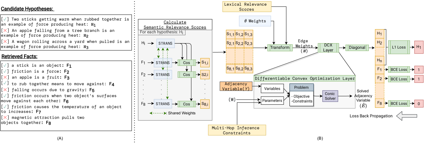
Figure 2: Overview of our approach: Illustrates the end-to-end architectural diagram of Diff-Explainer for the provided example.

The problem of Explainable Multi-Hop Question Answering can be stated as follows:

Definition 3.1 (Explanations in Multi-Hop Question Answering).

Given a question $Q$, answer $a$ and a knowledge base $F_{kb}$ (composed of natural language sentences), we say that we may infer hypothesis $h$ (where hypotheses $h$ is the concatenation of $Q$ with $a$) if there exists a subset ($F_{exp}$) of supporting facts $\{f_{1},f_{2},\ldots\}\subseteq F_{kb}$ of statements which would allow a human being to deduce $h$ from $\{f_{1},f_{2},\ldots\}$. We call this set of facts an explanation for $h$.

Given a question ($Q$) and a set of candidate answers $C=\{c_{1},~{}c_{2},~{}c_{3},...,~{}c_{n}\}$ ILP-based approaches Khashabi et al. (2016); Khot et al. (2017); Thayaparan et al. (2021) convert them into a list of hypothesis $H=\{h_{1},~{}h_{2},~{}h_{3},~{}\dots,~{}h_{n}\}$ by concatenating question and candidate answer. For each hypothesis $h_{i}$ these approaches typically adopt a retrieval model (e.g: BM25, FAISS Johnson et al. (2017)), to select a list of candidate explanatory facts $F=\{f_{1},~{}f_{2},~{}f_{3},~{}\dots,~{}f_{k}\}$, and construct a weighted graph $G=(V,E,W)$ with edge weights $W:E~{}\rightarrow~{}\mathbb{R}$ where $V=~{}\{\{h_{i}\}~{}\cup~{}F\}$, edge weight $W_{ik}$ of each edge $E_{ik}$ denote how relevant a fact $f_{k}$ is with respect to the hypothesis $h_{i}$.

Based on these definitions, ILP-based QA can be defined as follows:

Definition 3.2 (ILP-Based Multi-Hop QA).

Find a subset $V^{*}\subseteq V$, $h\in V^{*}$, $V^{*}\setminus\{h\}=F_{exp}$ and $E^{*}\subseteq E$ such that the induced subgraph $G^{*}=(V^{*},E^{*})$ is connected, weight $W[G^{*}=(V^{*},~{}E^{*})]:=\sum_{e\in E^{*}}W(e)$ is maximal and adheres to set of constraints $M_{c}$ designed to emulate multi-hop inference. The hypothesis $h_{i}$ with the highest subgraph weight $W[G^{*}=(V^{*},~{}E^{*})]$ is selected to be the correct answer $c_{ans}$.

The ILP-based inference has two main challenges in producing convincing explanations. First, design edge weights $W$, ideally capturing a quantification of the relevance of the fact to the hypothesis. Second, define constraints that emulate the multi-hop inference process.

3.1 Limitations with Existing ILP formulations

In previous work, the construction of the graph $G$ requires predetermined edge-weights based on lexical overlaps Khot et al. (2017) or semantic similarity using sentence embeddings Thayaparan et al. (2021), on top of which combinatorial optimization strategies are performed separately. From those approaches, ExplanationLP proposed by Thayaparan et al. (2021) is the only approach that modifies the graph weight function by optimizing the weight parameters $\theta$ by fine-tuning them for inference via Bayesian Optimization over pre-trained embeddings.

In contrast, we posit that learning the graph weights dynamically by fine-tuning the underlying neural embeddings towards answer and explanation selection will lead to more accurate and robust performance. To this end, the constraint optimization strategy should be differentiable and efficient. However, Integer Linear Programming based approaches present two critical shortcomings that prevent achieving this goal:

1. The Integer Linear Programming formulation operates with discrete inputs/outputs resulting in non-differentiability Paulus et al. (2021). Consequently, it cannot be integrated with deep neural networks and trained end-to-end. Making ILP differentiable requires non-trivial assumptions and approximations Paulus et al. (2021).

2. Integer Programming is known to be NP-complete, with the special case of 0-1 integer linear programming being one of Karp’s 21 NP-complete problems Karp (1972). Therefore, as the size of the combinatorial optimization problem increases, finding exact solutions becomes computationally intractable. This intractability is a strong limitation for multi-hop QA in general since these systems typically operate on large knowledge bases and corpora.

3.2 Subgraph Selection via Semi-Definite Programming

Differentiable convex optimization (DCX) layers Agrawal et al. (2019b) provide a way to encode constraints as part of a deep neural network. However, an ILP formulation is non-convex Wolsey (2020); Schrijver (1998) and cannot be incorporated into a differentiable convex optimization layer. The challenge is to approximate ILP with convex optimization constraints.

In order to alleviate this problem, we turn to Semi-Definite programming (SDP) Vandenberghe and Boyd (1996). SDP is non-linear but convex and has shown to efficiently approximate combinatorial problems.

A semi-definite optimization is a convex optimization of the form:

$$minimize C\cdot X$$ (1)

$$s.t A\cdot X=b_{i},~{}i=1,2,~{}\cdots,~{}m,$$ (2)

$$X\succeq 0,$$ (3)

Here $X\in\mathbb{S}^{n}$ is the optimization variable and $C,A_{1},\ldots,A_{p}\in\mathbb{S}^{n}$, and $b_{1},\ldots,b_{p}\in\mathbb{R}$. $X\succeq 0$ is a matrix inequality with $\mathbb{S}^{n}$ denotes a set of $n\times n$ symmetric matrices.

SDP is often used as a convex approximation of traditional NP-hard combinatorial graph optimization problems, such as the max-cut problem, the dense k-subgraph problem and the quadratic $\{0-1\}$ programming problem Lovász and Schrijver (1991).

Specifically, we adopt the semi-definite relaxation of the following quadratic $\{0,~{}1\}$ problem:

$$maximize y^{T}Wy$$ (4)

$$y\in\{0,1\}^{n}$$ (5)

Here $W$ is the edge weight matrix of the graph $G$ and the optimal solution for this problem $\hat{y}$ indicates if a node is part of the induced subgraph $G^{*}$.

We follow Helmberg (2000) in their reformulation and relaxation of this problem. Instead of vectors $y\in\{0,1\}^{n}$, we optimize over the set of positive semidefinite matrices satisfying the SDP constraint in the following relaxed convex optimization problem:

$$maximize \quad\langle W,Y\rangle$$ (6)

$$s.t Y-diag(Y)diag(Y)^{T}\succeq 0$$ (7)

where $\langle W,Y\rangle=\text{trace}(WY)$, $Y=yy^{T}$, $diag(Y)=y$.

The optimal solution for $Y$ in this problem $\hat{E}~{}\in~{}[0,~{}1]$ indicates if an edge is part of the subgraph $G^{*}$. In addition to the semi-definite constraints, we also impose Multi-hop inference constraints $M_{c}$. These constraints are introduced in Section 3.4 and the Appendix.

This reformulation provides the tightest approximation for the optimization with the convex constraints. Since this formulation is convex, we can now integrate it with differentiable convex optimization layers. Moreover, the semi-definite program relaxation can be solved by adopting the interior-point method De Klerk (2006); Vandenberghe and Boyd (1996) which has been proved to run in polynomial time Karmarkar (1984). To the best of our knowledge, we are the first to employ SDP to solve a natural language processing task.

3.3 Diff-Explainer: End-to-End Differentiable Architecture

Diff-Explainer is an end-to-end differentiable architecture that simultaneously solves the constraint optimization problem and dynamically adjusts the graph edge weights for better performance. We adopt differentiable convex optimization for the optimal subgraph selection problem. The complete architecture and setup are described in the subsequent subsections and Figure  2.

We transform a multi-hop question answering dataset into a multi-hop QA dataset by converting an example’s question ($q$) and the set of candidate answers $C=\{c_{1},~{}c_{2},~{}c_{3},~{}\dots,~{}c_{n}\}$ into hypotheses $H=\{h_{1},~{}h_{2},~{}h_{3},~{}\dots,~{}h_{n}\}$ (See Figure 2A) by using the approach proposed by Demszky et al. (2018). To build the initial graph, for the hypotheses set $H$ we adopt a retrieval model to select a list of candidate explanatory facts $F=\{f_{1},~{}f_{2},~{}f_{3},~{}\dots,~{}f_{k}\}$ to construct a weighted complete bipartite graph $G=(H,~{}F,~{}E,~{}W)$, where the weights $W_{ik}$ of each edge $E_{ik}$ denote how relevant a fact $f_{k}$ is with respect to the hypothesis $h_{i}$. Departing from traditional ILP approaches Thayaparan et al. (2021); Khashabi et al. (2018, 2016), the aim is to select the correct answer $c_{ans}$ and relevant explanations $F_{exp}$ with a single graph.

In order to demonstrate the impact of Diff-Explainer, we reproduce the formalization introduced by previous ILP solvers. Specifically, we approximate the two following solvers:

• TupleILP Khot et al. (2017): TupleILP constructs a semi-structured knowledge base using tuples extracted via Open Information Extraction (OIE) and performs inference over them. For example, in Figure 2A, $F1$ will be decomposed into (a stick; is a; object) and the subject (a stick) will be connected to the hypothesis to enforce constraints and build the subgraph.

• ExplanationLP Thayaparan et al. (2021): ExplanationLP classifies facts into abstract and grounding facts. Abstract facts are core scientific statements. Grounding facts help connect the generic terms in the abstract facts to the terms in the hypothesis. For example, in Figure 2A, $F_{1}$ is a grounding fact and helps to connect the hypothesis with the abstract fact $F_{7}$. The approach aims to emulate abstract reasoning.

Further details of these approaches can be found in the Appendix.

To demonstrate the impact of integrating a convex optimization layer into a broader end-to-end neural architecture, Diff-Explainer employs a transformer-based sentence embedding model. Figure 2B describes the end-to-end architectural diagram of Diff-Explainer. Specifically, we incorporate a differentiable convex optimization layer with Sentence-Transformer (STrans) Reimers et al. (2019), which has demonstrated state-of-the-art performance on semantic sentence similarity benchmarks.

STrans is adopted to estimate the relevance between hypothesis and facts during the construction of the initial graph. We use STrans as a bi-encoder architecture to minimize the computational overload and operate on large number of sentences. The semantic relevance score from STrans is complemented with a lexical relevance score computed considering the shared terms between hypotheses and facts. We calculate semantic and lexical relevance as follows:

Semantic Relevance ($s$): Given a hypothesis $h_{i}$ and fact $f_{j}$ we compute sentence vectors of $\vec{h_{i}}^{\,}=STrans(h_{i})$ and $\vec{f_{j}}^{\,}=STrans(f_{j})$ and calculate the semantic relevance score using cosine-similarity as follows:

$$\small s_{ij}=S(\vec{h_{i}}^{\,},~{}\vec{f_{j}}^{\,})=\frac{\vec{h_{i}}^{\,}\cdot\vec{f_{j}}^{\,}}{\|\vec{h_{i}}^{\,}\|\|\vec{f_{j}}^{\,}\|}$$ (8)

Lexical Relevance ($l$): The lexical relevance score of hypothesis $h_{i}$ and $f_{j}$ is given by the percentage of overlaps between unique terms (here, the function $trm$ extracts the lemmatized set of unique terms from the given text):

$$\small l_{ij}=L(h_{i},~{}f_{j})=\frac{|trm(h_{i})\cap trm(f_{j})|}{max(|trm(h_{i})|,|trm(f_{j})|)}$$ (9)

Given the above scoring function, we construct edge weights matrix ($W$) as follows:

$$\small W_{ij}=[\theta^{s}_{1},~{}\theta^{s}_{2},~{}\dots~{},\theta^{s}_{n}]\cdot[s_{ij}^{\mathcal{D}_{1}},~{}s_{ij}^{\mathcal{D}_{2}},~{}\dots~{},s_{ij}^{\mathcal{D}_{n}}]\\ +[\theta^{l}_{1},~{}\theta^{l}_{2},~{}\dots~{},\theta^{l}_{n}]\cdot[l_{ij}^{\mathcal{D}_{1}},~{}l_{ij}^{\mathcal{D}_{2}},~{}\dots~{},l_{ij}^{\mathcal{D}_{n}}]$$ (10)

Here relevance scores are weighted by weight parameters ($\theta$) with $\theta$ clamped to $[0,1]$. $s_{ij}^{\mathcal{D}_{k}}$ (or $l_{ij}^{\mathcal{D}_{k}}$) is $s_{ij}$ (or $l_{ij}$) if $(i,j)$ satisfy condition $\mathcal{D}_{k}$ or $0$ otherwise. TupleILP has two weights each for lexical and semantic relevance. Meanwhile, ExplanationLP has nine weights based on the type of fact and relevance type. Additional details on how to calculate $W$ for each approach can be found in the Appendix.

3.4 Answer and Explanation Selection

Given edge variable $Y$ and node variable $y$ ($diag(Y)=y$) (See Section 3.2) where 1 means the edge/node is part of the subgraph and 0 otherwise, we design the the answer selection constraint is defined as follows:

$$\sum_{i~{}\in~{}H}Y_{ii} =1$$ (11)

Each entry in the edge diagonal represents a value between 0 and 1, indicating whether the corresponding node in the initial graph should be included in the optimal subgraph.

Explanation selection is done via the following constraint that limits the number of nodes in the subgraph to be $m$.

$$\sum_{i~{}\in~{}V}Y_{ii} =m+1$$ (12)

Apart from these functional constraints, ILP based methods also impose semantic and structural constraints. For instance, ExplanationLP places explicit grounding-abstract fact chain constraints to perform efficient abstractive reasoning and TupleILP enforces constraints to leverage the SPO structure to align and select facts. See the Appendix on how these constraints are designed and imposed within Diff-Explainer.

The output from the DCX layer returns the solved edge adjacency matrix $\hat{E}$ with values between 0 and 1. We interpret the diagonal values of $\hat{E}$ be the probability of the specific node to be part of the selected subgraph. The final step is to optimize the sum of the L1 loss $l_{1}$ between the selected answer and correct answer $c_{ans}$ for the answer loss $\mathcal{L}_{ans}$:

$$\mathcal{L}_{ans}=l_{1}(diag(\hat{E})[h_{1},~{}h_{2},~{}\dots,~{}h_{n}],~{}c_{ans})$$ (13)

As well as the binary cross entropy loss $l_{b}$ between the selected explanatory facts and true explanatory facts $F_{exp}$ for the explanatory loss $\mathcal{L}_{exp}$:

$$\mathcal{L}_{exp}=l_{b}(diag(\hat{E})[f_{1},~{}f_{2},~{}\dots,~{}f_{k}],~{}F_{exp})$$ (14)

We add the losses to backpropagate to learn the $\theta$ weights and fine-tune the sentence transformers. The pseudo-code to train Diff-Explainer end-to-end is summarized in Algorithm 1.

Data: $M_{c}\leftarrow\textrm{Multi-hop inference constraints}$

Data: $Ans_{c}\leftarrow\textrm{Answer selection constraint}$

Data: $Exp_{c}\leftarrow\textrm{Explanation selection constraint}$

Data: $f_{w}\leftarrow\textrm{Graph weight function}$

$G\leftarrow\textrm{fact-graph-construction}(H,~{}F)$;

$l\leftarrow L(H,~{}F)$;

$\theta\leftarrow clamp([0,~{}1])$;

$epoch\leftarrow 0$;

while epoch $\leq$ max_epochs do

       $\vec{F}\leftarrow STrans(F)$;

       $\vec{H}\leftarrow STrans(H)$;

       $s\leftarrow S(\vec{H},~{}\vec{F})$;

       $W\leftarrow f_{w}(s,~{}l;~{}\theta)$;

       $\hat{E}\leftarrow DCX(W,~{}\{M_{c},~{}Ans_{c},~{}Exp_{c}\})$;

      

      $\hat{V}\leftarrow diag(\hat{E})$;

       $\mathcal{L}_{ans}\leftarrow l_{1}(\hat{V}[h_{1},~{}h_{2},~{}\dots,~{}h_{n}],~{}c_{ans})$;

       if $F_{exp}$ is available then

             $\mathcal{L}_{exp}\leftarrow l_{b}(\hat{V}[f_{1},~{}f_{2},~{}\dots,~{}f_{k}],~{}F_{exp})$;

             $loss=\mathcal{L}_{ans}+\mathcal{L}_{exp}$;

            

      else

             $loss=\mathcal{L}_{ans}$;

            

       end if

      update $\theta$, $STrans$ using AdamW optimizer by minimizing $loss$;

       $epoch\leftarrow epoch+1$;

      

end while

Result: Store best $\theta$ and $STrans$

Algorithm 1 Training Diff-Explainer

4 Empirical Evaluation

Question Sets:

We use the following multiple-choice question sets to evaluate the Diff-Explainer.

(1) WorldTree Corpus Xie et al. (2020): The 4,400 question and explanations in the WorldTree corpus are split into three different subsets: train-set, dev-set and test-set. We use the dev-set to assess the explainability performance since the explanations for test-set are not publicly available.

(2) ARC-Challenge Corpus Clark et al. (2018): ARC-Challenge is a multiple-choice question dataset which consists of question from science exams from grade 3 to grade 9. These questions have proven to be challenging to answer for other LP-based question answering and neural approaches.

Experimental Setup

: We use all-mpnet-base-v2 model as the Sentence Transformer model for the sentence representation in Diff-Explainer. The motivation to choose this model is to use a pre-trained model on natural language inference and MPNet_Base Song et al. (2020) is smaller compared to large models like BERT_Large, enabling us to encode a larger number of facts. Similarly, for fact retrieval representation, we use all-mpnet-base-v2 trained with gold explanations of WorldTree Corpus to achieve a Mean Average Precision of 40.11 in the dev-set. We cache all the facts from the background knowledge and retrieve the top $k$ facts using MIPS retrieval Johnson et al. (2017). We follow a similar setting proposed by Thayaparan et al. (2021) for the background knowledge base by combining over 5000 abstract facts from the WorldTree table store (WTree) and over 100,000 is-a grounding facts from ConceptNet (CNet) Speer et al. (2016). Furthermore, we also set $m$=2 in line with the previous configurations from TupleILP and ExplanationLP.

Baselines:

In order to assess the complexity of the task and the potential benefits of the convex optimization layers presented in our approach, we show the results for different baselines. We run all models with $k=\{1,\ldots,10,25,50,75,100\}$ to find the optimal setting for each baseline and perform a fair comparison. For each question, the baselines take as input a set of hypotheses, where each hypothesis is associated with $k$ facts, ranked according to the fact retrieval model.

(1) IR Solver Clark et al. (2018): This approach attempts to answer the questions by computing the accumulated score from all $k$ obtained from summing up the retrieval scores. In this case, the retrieval scores are calculated using the cosine similarity of fact and hypothesis sentence vectors obtained from the STrans model trained on gold explanations. The hypothesis associated with the highest score is selected as the one containing the correct answer.

(2) BERT_Base and BERT_Large Devlin et al. (2019): To use BERT for this task, we concatenate every hypothesis with $k$ retrieved facts, using the separator token [SEP]. We use the HuggingFace Wolf et al. (2019) implementation of BertForSequenceClassification, taking the prediction with the highest probability for the positive class as the correct answer.

(3) PathNet Kundu et al. (2019): PathNet is a graph-based neural approach that constructs a single linear path composed of two facts connected via entity pairs for reasoning. It uses the constructed paths as evidence of its reasoning process. They have exhibited strong performance for multiple-choice science questions.

(4) TupleILP and ExplanationLP: Both replications of the non-differentiable solvers are implemented with the same constraints as Diff-Explainer via SDP approximation without fine-tuning end-to-end; instead, we fine-tune the $\theta$ parameters using Bayesian optimization and frozen STrans representations. This baseline helps us to understand the impact of the end-to-end fine-tuning.

4.1 Answer Selection

WorldTree Corpus:

Table 1 presents the answer selection performance on the WorldTree corpus in terms of accuracy, presenting the best results obtained for each model after testing for different values of $k$. We also include the results for BERT without explanation in order to evaluate the influence extra facts can have on the final score. We also present the results for two different training goals, optimizing for only the answer and optimizing jointly for answer and explanation selection.

Model	Acc
Baselines
IR Solver	50.48
BERTBase (Without Retrieval)	45.43
BERTBase	58.06
BERTLarge (Without Retrieval)	49.63
BERTLarge	59.32
TupleILP	49.81
ExplanationLP	62.57
PathNet	43.40
Diff-Explainer
TupleILP constraints
- Answer Selection only	61.13
- Answer and explanation selection	63.11
ExplanationLP constraints
- Answer selection only	69.73
- Answer and explanation selection	71.48

Table 1: Answer selection performance for the baselines and across different configurations of our approach on WorldTree Corpus.

We draw the following conclusions from the empirical results obtained on the WorldTree corpus (The performance increase here are in expressed absolute terms):

(1) Diff-Explainer with ExplanationLP and TupleILP outperforms the respective non-differentiable solvers by 13.3% and 8.91%. This increase in performance indicates that Diff-Explainer can incorporate different types of constraints and significantly improve performance compared with the non-differentiable version.

(2) It is evident from the performance obtained by a large model such as BERT_Large (59.32%) that we are dealing with a non-trivial task. The best Diff-Explainer setting (with ExplanationLP) outperforms the best transformer-based models with and without explanations by 12.16% and 21.85%. Additionally, we can also observe that both with TupleILP and ExplanationLP, we obtain better scores over the transformer-based configurations.

(3) Fine-tuning with explanations yielded better performance than only answer selection with ExplanationLP and TupleILP, improving performance by 1.75% and 1.98%. The increase in performance indicates that Diff-Explainer can learn from the distant supervision of answer selection and improve in a strong supervision setting.

(4) Overall, we can conclude that incorporating constraints using differentiable convex optimization with transformers for multi-hop QA leads to better performance than pure constraint-based or transformer-only approaches.

ARC Corpus:

Table 2 presents a comparison of baselines and our approach with different background knowledge bases: TupleInf, the same as used by TupleILP Khot et al. (2017), and WorldTree & ConceptNet as used by ExplanationLP Thayaparan et al. (2021). We have also reported the original scores reported by the respective approaches.

For this dataset, we use our approach with the same settings as the model applied to WorldTree, and fine-tune for only answer selection since ARC does not have gold explanations. Models employing Large Language Models (LLMs) trained across multiple question answering datasets like UnifiedQA Khashabi et al. (2020) and AristoBERT Xu et al. (2021) have demonstrated strong performance in ARC with an accuracy of 81.14 and 68.95 respectively.

To ensure a fair comparison, we only compare the best configuration of Diff-Explainer with other approaches that have been trained only on the ARC corpus and provide some form of explanations in Table 3. Here the explainability column indicates if the model delivers an explanation for the predicted answer. A subset of the approaches produces evidence for the answer but remains intrinsically black-box. These models have been marked as Partial.

(1) Diff-Explainer improves the performance of non-differentiable solvers regardless of the background knowledge and constraints. With the same background knowledge, our model improves the original TupleILP and ExplanationLP by 10.12% and 2.74%, respectively.

(2) Our approach also achieves the highest performance for partially and fully explainable approaches trained only on ARC corpus.

(3) As illustrated in Table 3, we outperform the next best fully explainable baseline (ExplanationLP) by 2.74%. We also outperform the stat-of-the-art model AutoRocc Yadav et al. (2019b) (uses BERT_Large) that is only trained on ARC corpus by 1.71% with 230 million fewer parameters.

(4) Overall, we achieve consistent performance improvement over different knowledge bases (TupleInf, Wordtree & ConceptNet) and question sets (ARC, WorldTree), indicating that the robustness of the approach.

Model	Background KB	Acc
TupleILP  Khot et al. (2017)	TupleInf	23.83
ExplanationLP Thayaparan et al. (2021)	WTree & CNet	40.21
TupleILP (Ours)	TupleInf	29.12
ExplanationLP (Ours)	WTree & CNet	37.40
Diff-Explainer
TupleILP Constraints	TupleInf	33.95
ExplanationLP Constraints	WTree & CNet	42.95

Table 2: Answer Selection performance on ARC corpus with Diff-Explainer fine-tuned on answer selection.

Model	Explainable	Accuracy
BERTLarge	No	35.11
IR Solver Clark et al. (2016)	Yes	20.26
TupleILP Khot et al. (2017)	Yes	23.83
TableILP Khashabi et al. (2016)	Yes	26.97
ExplanationLP  Thayaparan et al. (2021)	Yes	40.21
DGEM Clark et al. (2016)	Partial	27.11
KG2 Zhang et al. (2018)	Partial	31.70
ET-RR Ni et al. (2019)	Partial	36.61
Unsupervised AHE Yadav et al. (2019a)	Partial	33.87
Supervised AHE Yadav et al. (2019a)	Partial	34.47
AutoRocc Yadav et al. (2019b)	Partial	41.24
Diff-Explainer (ExplanationLP)	Yes	42.95

Table 3: ARC challenge scores compared with other Fully or Partially explainable approaches trained only on the ARC dataset.

4.2 Explanation Selection

Table 4 shows the Precision@K scores for explanation retrieval for PathNet, ExplanationLP/TupleILP and Diff-Explainer with ExplanationLP/TupleILP trained on answer and explanation selection. We choose Precision@K as the evaluation metric as the design of the approaches is not to construct full explanations but to take the top $k$=2 explanations and select the answer.

As evident from the table, our approach significantly outperforms PathNet. We also improved the explanation selection performance over the non-differentiable solvers indicating the end-to-end fine-tuning also helps improve the selection of explanatory facts.

Model	Precision@1	Precision@2
TupleILP	40.44	31.21
ExplanationLP	51.99	40.41
PathNet	19.79	13.73
Diff-Explainer
TupleILP (Best)	40.64	32.23
ExplanationLP (Best)	56.77	41.91

Table 4: F1 score for explanation selection in WorldTree dev-set .

4.3 Answer Selection with Increasing Distractors

Question (1): Fanning can make a wood fire burn hotter because the fanning: Correct Answer: adds more oxygen needed for burning.

PathNet

Answer: provides the energy needed to keep the fire going. Explanations: (i) fanning a fire increases the oxygen near the fire, (ii) placing a heavy blanket over a fire can be used to keep oxygen from reaching a fire

ExplanationLP

Answer: increases the amount of wood there is to burn. Explanations: (i) more burning causes fire to be hotter, (ii) wood burns

Diff-Explainer ExplanationLP

Answer: adds more oxygen needed for burning. Explanations: (i) more burning causes fire to be hotter, (ii) fanning a fire increases the oxygen near the fire

Question (2): Which type of graph would best display the changes in temperature over a 24 hour period? Correct Answer: line graph.

PathNet

Answer: circle/pie graph. Explanations: (i) a line graph is used for showing change ; data over time

ExplanationLP

Answer: circle/pie graph. Explanations: (i) 1 day is equal to 24 hours, (ii) a circle graph; pie graph can be used to display percents; ratios

Diff-Explainer ExplanationLP

Answer: line graph. Explanations: (i) a line graph is used for showing change; data over time, (ii) 1 day is equal to 24 hours

Question (3): Why has only one-half of the Moon ever been observed from Earth? Correct Answer: The Moon rotates at the same rate that it revolves around Earth..

PathNet

Answer: The Moon has phases that coincide with its rate of rotation. Explanations: (i) the moon revolving around ; orbiting the Earth causes the phases of the moon, (ii) a new moon occurs 14 days after a full moon

ExplanationLP

Answer: The Moon does not rotate on its axis. Explanations: (i) the moon rotates on its axis, (ii) the dark half of the moon is not visible

Diff-Explainer ExplanationLP

Answer: The Moon is not visible during the day. Explanations: (i) the dark half of the moon is not visible, (ii) a complete revolution; orbit of the moon around the Earth takes 1; one month

Table 5: Example of predicted answers and explanations (Only CENTRAL explanations) obtained from our model with different levels of fine-tuning.

As noted by previous works Yadav et al. (2019b, 2020), the answer selection performance can decrease when increasing the number of used facts $k$ for Transformer. We evaluate how our approach stacks compared with transformer-based approaches in this aspect, presented in Figure 3.

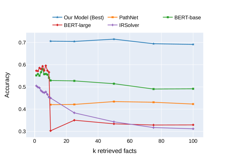
Figure 3: Comparison of accuracy for different number of retrieved facts.

As we can see, the IR Solver decreases in performance as we add more facts, while the scores for transformer-based models start deteriorating for $k>5$. Such results might seem counter-intuitive since it would be natural to expect a model’s performance to increase as we add supporting facts. However, in practice, that does not apply as by adding more facts, there is an addition of distractors that such models may not filter out.

We can prominently see this for BERT_Large with a sudden drop in performance for $k=10$, going from 56.61 to 30.26. Such drop is likely being caused by substantial overfitting; with the added noise, the model partially lost the ability for generalization. A softer version of this phenomenon is also observed for BERT_Base.

In contrast, our model’s performance increases as we add more facts, reaching a stable point around $k=50$. Such performance stems from our combination of overlap and relevance scores along with the structural and semantic constraints. The obtained results highlight our model’s robustness to distracting knowledge, allowing its use in data-rich scenarios, where one needs to use facts from extensive knowledge bases. PathNet is also exhibiting robustness across increasing distractors, but we consistently outperform it across all $k$ configurations.

On the other hand, for smaller values of $k$ our model is outperformed by transformer-based approaches, hinting that our model is more suitable for scenarios involving large knowledge bases such as the one presented in this work.

4.4 Qualitative Analysis

We selected some qualitative examples that showcase how end-to-end fine-tuning can improve the quality and inference and presented them in Table 5. We use the ExplanationLP for non-differentiable solver and Diff-Explainer as they yield higher performance in answer and explanation selection.

For Question (1), Diff-Explainer retrieves both explanations correctly and be able to answer correctly. Both PathNet and ExplanationLP has correctly retrieved at least one explanation but performed incorrect inference. We hypothesise that the other two approaches were distracted by the lexical overlaps in question/answer and facts, while our approach is robust towards distractor terms. In Question (2), our model was able only to retrieve one explanation correctly and was distracted by the lexical overlap to retrieve an irrelevant one. However, it still was able to answer correctly. In Question (3), all the approaches answered the question wrong, including our approach. Even though our approach was able to retrieve at least one correct explanation, it was not able to combine the information to answer and was distracted by lexical noise. These shortcomings indicate that more work can be done, and different constraints can be experimented with for combining facts.

5 Conclusion

We presented a novel framework for encoding explicit and controllable assumptions as an end-to-end learning framework for question answering. We empirically demonstrated how incorporating these constraints in broader Transformer-based architectures can improve answer and explanation selection. The presented framework adopts constraints from TupleILP and ExplanationLP, but Diff-Explainer can be extended to encode different constraints with varying degrees of complexity.

This approach can also be extended to handle other forms of multi-hop QA, including open-domain, cloze style and answer generation. ILP has also been employed for relation extraction Roth and Yih (2004); Choi et al. (2006); Chen et al. (2014), semantic role labeling Punyakanok et al. (2004); Koomen et al. (2005), sentiment analysis Choi and Cardie (2009) and explanation regeneration Gupta and Srinivasaraghavan (2020). We can adapt and improve the constraints presented in this approach to build explainable approaches for the respective tasks.

Diff-Explainer is the first work investigating the intersection of explicit constraints and latent neural representations to the best of our knowledge. We hope this work will open the way for future lines of research on neuro-symbolic models, leading to more controllable, transparent and explainable NLP models.

6 Appendix

6.1 Model Description

This section presents a detailed explanation of TupleILP and ExplanationLP:

TupleILP

TupleILP uses Subject-Predicate-Object tuples for aligning and constructing the explanation graph. As shown in Figure 4C, the tuple graph is constructed and lexical overlaps are aligned to select the explanatory facts. The constraints are designed based on the position of text in the tuple.

ExplanationLP

Given hypothesis $H_{1}$ from Figure 4A, the underlying concept the hypothesis attempts to test is the understanding of friction. Different ILP approaches would attempt to build explanation graph differently. For example, ExplanationLP Thayaparan et al. (2021) would classify core scientific facts ($F_{6}$-$F_{8}$) into abstract facts and the linking facts ($F_{1}$-$F_{5}$) that connects generic or abstract terms in the hypothesis into grounding fact. The constraints are designed to emulate abstraction by starting to from the concrete statement to more abstract concepts via the grounding facts as shown in Figure 4B.

Figure 4: ILP-Based Natural Language Inference

6.2 Objective Function

In this section, we explain how to design the objective function for TupleILP and ExplanationLP to adopt with Diff-Explainer.

Given $n$ candidate hypotheses and $k$ candidate explanatory facts, $A$ represents an adjacency matrix of dimension $((n+k)\times(n+k))$ where the first $n$ columns and rows denote the candidate hypotheses, while the remaining rows and columns represent the candidate explanatory facts. The adjacency matrix denotes the graph’s lexical connections between hypotheses and facts. Specifically, each entry in the matrix $A_{ij}$ contains the following values:

$$\small A{ij}=\begin{cases}1,&i\leq n,j>n,~{}|trm(h_{i})\cap trm(f_{j-n})|>0\\ 1,&j\leq n,i>n,~{}|trm(h_{j})\cap trm(f_{i-n})|>0\\ 0,&\text{otherwise}\end{cases}$$ (15)

Description	DPP Format	Parameters
TupleILP
Sub graph must have $\leq w_{1}$ active tuples	$$\sum_{i~{}\in~{}F}Y_{ii}\leq w_{1}+1$$ (16)	-
Active hypothesis term must have $\leq w_{2}$ edges	$$H_{\theta}[:,:,i]\odot Y\leq w_{2}\quad\forall i~{}\in H^{t}$$ (17)	$H_{\theta}$ is populated by hypothesis term matrix $H$ with dimension $((n+k)\times(n+k)\times l)$ and the values are given by: $$H_{ijk}=\begin{cases}1,&\parbox[t]{156.49014pt}{$\forall~{}k\in H^{t},i\in H,j\in F,\\ t_{k}\in trm(h_{i}),t_{k}\in trm(f_{j})$}\\ 1,&\parbox[t]{156.49014pt}{$\forall~{}k\in H^{t},i\in F,j\in H,\\ t_{k}\in trm(h_{j}),t_{k}\in trm(f_{i})$}\\ 0,&\text{otherwise}\end{cases}$$ (18)
Active tuple must have active subject	$$Y\odot T^{S}_{\theta}>=E\odot A_{\theta}$$ (19)	$A_{\theta}$ populated by adjacency matrix $A$, $T^{S}_{\theta}$ by subject tuple matrix $T^{S}$ with dimension $((n+k)\times(n+k))$ and the values are given by: $$T^{S}_{ij}=\begin{cases}1,&\parbox[t]{156.49014pt}{$i\in H,~{}j\in F,\\ |trm(h_{i})\cap trm(f^{S}_{j})|>0$ }\\ 1,&\parbox[t]{156.49014pt}{$i\in F,~{}j\in H,\\ |trm(h_{j})\cap trm(f^{S}_{i})|>0$ }\\ 0,&\text{otherwise}\end{cases}$$ (20)
Active tuple must have $\geq w_{3}$ active fields	$$Y\odot T^{S}_{\theta}+Y\odot T^{P}_{\theta}+Y\odot T^{O}_{\theta}\geq w_{3}(Y\odot A_{\theta})$$ (21)	$A_{\theta}$ populated by adjacency matrix $A$ and $T^{S}_{\theta}$, $T^{P}_{\theta}$, $T^{O}_{\theta}$ populated by subject, predicate and object matrices $T^{S}$, $T^{P}$, $T^{O}$ respectively. Predicate and object tuples are converted into $T^{P},~{}T^{O}$ matrices similar to $T^{S}$
Active tuple must have an edge to some hypothesis term	Implemented during graph construction by only considering tuples that have lexical overlap with a hypothesis	-
ExplanationLP
Limits the total number of abstract facts to $w_{4}$	$$diag(Y)\cdot F^{AB}_{\theta}\leq w_{4}$$ (22)	$F^{AB}_{\theta}$ is populated by Abstract fact matrix $F^{AB}$, where: $$F^{AB}_{ij}=\begin{cases}1,&\parbox[t]{156.49014pt}{$i\in H,~{}j\in F^{A}$}\\ 0,&\text{otherwise}\end{cases}$$ (23)

Table 6: Adopting TupleILP and ExplanationLP constraints in DPP format. For this work we set the hyperparameters $w_{1}$=2, $w_{2}$=2, $w_{3}$=1 and $w_{4}$=2

Given the relevance scoring functions, we construct edge weights matrix ($W$) via a weighted function for each approach as follows:

TupleILP

The weight function for Diff-Explainer with TupleILP constraints is:

$$\small W_{ij}=(\theta_{s_{r}}S_{ij}+\theta_{l_{r}}L_{ij})\times A_{ij}~{}\forall i,j\in V$$ (24)

ExplanationLP

Give Abstract KB ($F_{A})$ and Grounding KB ($F_{G})$, the weight function for Diff-Explainer with Explanation LP is as follows:

6.3 Constraints with Disciplined Parameterized Programming (DPP)

In order to adopt differentiable convex optimization layers, the constraints should be defined following the Disciplined Parameterized Programming (DPP) formalism Agrawal et al. (2019b), providing a set of conventions when constructing convex optimization problems. DPP consists of functions (or atoms) with a known curvature (affine, convex or concave) and per-argument monotonicities. In addition to these, DPP also consists of Parameters which are symbolic constants with an unknown numerical value assigned during the solver run.

TupleILP

We extract SPO tuples $f^{t}_{i}=\{f^{S}_{i},~{}f^{P}_{i},~{}f^{O}_{i}\}$ for each fact $f_{i}$ using an Open Information Extraction model Stanovsky et al. (2018). From the hypothesis $h_{i}$ we extract the set of unique terms $h^{ht}_{i}=\{t^{h_{i}}_{1},~{}t^{h_{i}}_{2},~{}t^{h_{i}}_{3},~{}\dots,~{}t^{h_{i}}_{l}\}$ excluding stopwords.

In addition to the aforementioned constraints and semidefinite constraints specified in Equation 7, we adopt part of the constraints from TupleILP Khot et al. (2017). In order to implement TupleILP constraints, we extract SPO tuples $f^{t}_{i}=\{f^{S}_{i},~{}f^{P}_{i},~{}f^{O}_{i}\}$ for each fact $f_{i}$ using an Open Information Extraction model Stanovsky et al. (2018). From the hypotheses $H$ we also extract the set of unique terms $H^{t}=\{t_{1},~{}t_{2},~{}t_{3},~{}\dots,~{}t_{l}\}$ excluding stopwords. The constraints are described in Table 6.

ExplanationLP

ExplanationLP constraints are described in Table 6.

References

- Agrawal et al. (2019a) A. Agrawal, S. Barratt, S. Boyd, E. Busseti, and W. Moursi. 2019a. Differentiating through a cone program. Journal of Applied and Numerical Optimization, 1(2):107–115.
- Agrawal et al. (2019b) Akshay Agrawal, Brandon Amos, Shane Barratt, Stephen Boyd, Steven Diamond, and J. Zico Kolter. 2019b. Differentiable convex optimization layers. In Advances in Neural Information Processing Systems, volume 32. Curran Associates, Inc.
- Amos and Kolter (2017) Brandon Amos and J Zico Kolter. 2017. Optnet: Differentiable optimization as a layer in neural networks. In International Conference on Machine Learning, pages 136–145. PMLR.
- Busseti et al. (2019) Enzo Busseti, Walaa M Moursi, and Stephen Boyd. 2019. Solution refinement at regular points of conic problems. Computational Optimization and Applications, 74(3):627–643.
- Chen et al. (2014) Liwei Chen, Yansong Feng, Songfang Huang, Yong Qin, and Dongyan Zhao. 2014. Encoding relation requirements for relation extraction via joint inference. In Proceedings of the 52nd Annual Meeting of the Association for Computational Linguistics (Volume 1: Long Papers), pages 818–827, Baltimore, Maryland. Association for Computational Linguistics.
- Choi et al. (2006) Yejin Choi, Eric Breck, and Claire Cardie. 2006. Joint extraction of entities and relations for opinion recognition. In Proceedings of the 2006 Conference on Empirical Methods in Natural Language Processing, pages 431–439, Sydney, Australia. Association for Computational Linguistics.
- Choi and Cardie (2009) Yejin Choi and Claire Cardie. 2009. Adapting a polarity lexicon using integer linear programming for domain-specific sentiment classification. In Proceedings of the 2009 conference on empirical methods in natural language processing, pages 590–598.
- Clark et al. (2018) Peter Clark, Isaac Cowhey, Oren Etzioni, Tushar Khot, Ashish Sabharwal, Carissa Schoenick, and Oyvind Tafjord. 2018. Think you have solved question answering? try arc, the ai2 reasoning challenge. arXiv preprint arXiv:1803.05457.
- Clark et al. (2016) Peter Clark, Oren Etzioni, Tushar Khot, Ashish Sabharwal, Oyvind Tafjord, Peter D Turney, and Daniel Khashabi. 2016. Combining retrieval, statistics, and inference to answer elementary science questions. In AAAI, pages 2580–2586. Citeseer.
- Clark et al. (2021) Peter Clark, Oyvind Tafjord, and Kyle Richardson. 2021. Transformers as soft reasoners over language. In Proceedings of the Twenty-Ninth International Conference on International Joint Conferences on Artificial Intelligence, pages 3882–3890.
- De Klerk (2006) Etienne De Klerk. 2006. Aspects of semidefinite programming: interior point algorithms and selected applications, volume 65. Springer Science & Business Media.
- Demszky et al. (2018) Dorottya Demszky, Kelvin Guu, and Percy Liang. 2018. Transforming question answering datasets into natural language inference datasets. arXiv preprint arXiv:1809.02922.
- Devlin et al. (2019) Jacob Devlin, Ming-Wei Chang, Kenton Lee, and Kristina Toutanova. 2019. Bert: Pre-training of deep bidirectional transformers for language understanding. In Proceedings of the 2019 Conference of the North American Chapter of the Association for Computational Linguistics: Human Language Technologies, Volume 1 (Long and Short Papers), pages 4171–4186.
- Djolonga and Krause (2017) Josip Djolonga and Andreas Krause. 2017. Differentiable learning of submodular models. Advances in Neural Information Processing Systems, 30:1013–1023.
- Donti et al. (2017) Priya L Donti, Brandon Amos, and J Zico Kolter. 2017. Task-based end-to-end model learning in stochastic optimization. arXiv preprint arXiv:1703.04529.
- Gontier et al. (2020) Nicolas Gontier, Koustuv Sinha, Siva Reddy, and Chris Pal. 2020. Measuring systematic generalization in neural proof generation with transformers. Advances in Neural Information Processing Systems, 33:22231–22242.
- Guidotti et al. (2018) Riccardo Guidotti, Anna Monreale, Salvatore Ruggieri, Franco Turini, Fosca Giannotti, and Dino Pedreschi. 2018. A survey of methods for explaining black box models. ACM computing surveys (CSUR), 51(5):1–42.
- Gupta and Srinivasaraghavan (2020) Aayushee Gupta and Gopalakrishnan Srinivasaraghavan. 2020. Explanation regeneration via multi-hop ILP inference over knowledge base. In Proceedings of the Graph-based Methods for Natural Language Processing (TextGraphs), pages 109–114, Barcelona, Spain (Online). Association for Computational Linguistics.
- Helmberg (2000) Christoph Helmberg. 2000. Semidefinite programming for combinatorial optimization.
- Jansen (2018) Peter Jansen. 2018. Multi-hop inference for sentence-level textgraphs: How challenging is meaningfully combining information for science question answering? arXiv preprint arXiv:1805.11267.
- Jansen et al. (2021) Peter Jansen, Mokanarangan Thayaparan, Marco Valentino, and Dmitry Ustalov. 2021. Textgraphs 2021 shared task on multi-hop inference for explanation regeneration. In Proceedings of the Fifteenth Workshop on Graph-Based Methods for Natural Language Processing (TextGraphs-15).
- Jansen et al. (2018) Peter Jansen, Elizabeth Wainwright, Steven Marmorstein, and Clayton Morrison. 2018. Worldtree: A corpus of explanation graphs for elementary science questions supporting multi-hop inference. In Proceedings of the Eleventh International Conference on Language Resources and Evaluation (LREC 2018).
- Johnson et al. (2017) Jeff Johnson, Matthijs Douze, and Hervé Jégou. 2017. Billion-scale similarity search with gpus. CoRR, abs/1702.08734.
- Karmarkar (1984) Narendra Karmarkar. 1984. A new polynomial-time algorithm for linear programming. In Proceedings of the sixteenth annual ACM symposium on Theory of computing, pages 302–311.
- Karp (1972) Richard M Karp. 1972. Reducibility among combinatorial problems. In Complexity of computer computations, pages 85–103. Springer.
- Khashabi et al. (2016) Daniel Khashabi, Tushar Khot, Ashish Sabharwal, Peter Clark, Oren Etzioni, and Dan Roth. 2016. Question answering via integer programming over semi-structured knowledge. In Proceedings of the Twenty-Fifth International Joint Conference on Artificial Intelligence, pages 1145–1152.
- Khashabi et al. (2018) Daniel Khashabi, Tushar Khot, Ashish Sabharwal, and Dan Roth. 2018. Question answering as global reasoning over semantic abstractions. In Proceedings of the AAAI Conference on Artificial Intelligence, volume 32.
- Khashabi et al. (2020) Daniel Khashabi, Sewon Min, Tushar Khot, Ashish Sabharwal, Oyvind Tafjord, Peter Clark, and Hannaneh Hajishirzi. 2020. Unifiedqa: Crossing format boundaries with a single qa system. arXiv preprint arXiv:2005.00700.
- Khot et al. (2020) Tushar Khot, Peter Clark, Michal Guerquin, Peter Jansen, and Ashish Sabharwal. 2020. Qasc: A dataset for question answering via sentence composition. In Proceedings of the AAAI Conference on Artificial Intelligence, volume 34, pages 8082–8090.
- Khot et al. (2017) Tushar Khot, Ashish Sabharwal, and Peter Clark. 2017. Answering complex questions using open information extraction. arXiv preprint arXiv:1704.05572.
- Koomen et al. (2005) Peter Koomen, Vasin Punyakanok, Dan Roth, and Wen-tau Yih. 2005. Generalized inference with multiple semantic role labeling systems. In Proceedings of the Ninth Conference on Computational Natural Language Learning (CoNLL-2005), pages 181–184.
- Kundu et al. (2019) Souvik Kundu, Tushar Khot, Ashish Sabharwal, and Peter Clark. 2019. Exploiting explicit paths for multi-hop reading comprehension. In Proceedings of the 57th Annual Meeting of the Association for Computational Linguistics, pages 2737–2747, Florence, Italy. Association for Computational Linguistics.
- Liang et al. (2021) Yu Liang, Siguang Li, Chungang Yan, Maozhen Li, and Changjun Jiang. 2021. Explaining the black-box model: A survey of local interpretation methods for deep neural networks. Neurocomputing, 419:168–182.
- Lovász and Schrijver (1991) L. Lovász and A. Schrijver. 1991. Cones of matrices and set-functions and 0-1 optimization. SIAM JOURNAL ON OPTIMIZATION, 1:166–190.
- Ni et al. (2019) Jianmo Ni, Chenguang Zhu, Weizhu Chen, and Julian McAuley. 2019. Learning to attend on essential terms: An enhanced retriever-reader model for open-domain question answering. In Proceedings of the 2019 Conference of the North American Chapter of the Association for Computational Linguistics: Human Language Technologies, Volume 1 (Long and Short Papers), pages 335–344.
- O’Donoghue (2021) Brendan O’Donoghue. 2021. Operator splitting for a homogeneous embedding of the linear complementarity problem. SIAM Journal on Optimization, 31:1999–2023.
- Paulus et al. (2021) Anselm Paulus, Michal Rolínek, Vít Musil, Brandon Amos, and Georg Martius. 2021. Comboptnet: Fit the right np-hard problem by learning integer programming constraints. CoRR, abs/2105.02343.
- Punyakanok et al. (2004) Vasin Punyakanok, Dan Roth, Wen-tau Yih, and Dav Zimak. 2004. Semantic role labeling via integer linear programming inference. In COLING 2004: Proceedings of the 20th International Conference on Computational Linguistics, pages 1346–1352, Geneva, Switzerland. COLING.
- Reimers et al. (2019) Nils Reimers, Iryna Gurevych, Nils Reimers, Iryna Gurevych, Nandan Thakur, Nils Reimers, Johannes Daxenberger, and Iryna Gurevych. 2019. Sentence-bert: Sentence embeddings using siamese bert-networks. In Proceedings of the 2019 Conference on Empirical Methods in Natural Language Processing. Association for Computational Linguistics.
- Roth and Yih (2004) Dan Roth and Wen-tau Yih. 2004. A linear programming formulation for global inference in natural language tasks. In Proceedings of the Eighth Conference on Computational Natural Language Learning (CoNLL-2004) at HLT-NAACL 2004, pages 1–8, Boston, Massachusetts, USA. Association for Computational Linguistics.
- Rudin (2019) Cynthia Rudin. 2019. Stop explaining black box machine learning models for high stakes decisions and use interpretable models instead. Nature Machine Intelligence, 1(5):206–215.
- Saha et al. (2020) Swarnadeep Saha, Sayan Ghosh, Shashank Srivastava, and Mohit Bansal. 2020. Prover: Proof generation for interpretable reasoning over rules. In Proceedings of the 2020 Conference on Empirical Methods in Natural Language Processing (EMNLP), pages 122–136.
- Schrijver (1998) Alexander Schrijver. 1998. Theory of linear and integer programming. John Wiley & Sons.
- Song et al. (2020) Kaitao Song, Xu Tan, Tao Qin, Jianfeng Lu, and Tie-Yan Liu. 2020. Mpnet: Masked and permuted pre-training for language understanding. CoRR, abs/2004.09297.
- Speer et al. (2016) Robyn Speer, Joshua Chin, and Catherine Havasi. 2016. Conceptnet 5.5: An open multilingual graph of general knowledge. CoRR, abs/1612.03975.
- Stanovsky et al. (2018) Gabriel Stanovsky, Julian Michael, Luke Zettlemoyer, and Ido Dagan. 2018. Supervised open information extraction. In Proceedings of the 2018 Conference of the North American Chapter of the Association for Computational Linguistics: Human Language Technologies, Volume 1 (Long Papers), pages 885–895, New Orleans, Louisiana. Association for Computational Linguistics.
- Tafjord et al. (2021) Oyvind Tafjord, Bhavana Dalvi, and Peter Clark. 2021. Proofwriter: Generating implications, proofs, and abductive statements over natural language. In Findings of the Association for Computational Linguistics: ACL-IJCNLP 2021, pages 3621–3634.
- Thayaparan et al. (2020) Mokanarangan Thayaparan, Marco Valentino, and André Freitas. 2020. A survey on explainability in machine reading comprehension. arXiv preprint arXiv:2010.00389.
- Thayaparan et al. (2021) Mokanarangan Thayaparan, Marco Valentino, and André Freitas. 2021. Explainable inference over grounding-abstract chains for science questions. In Findings of the Association for Computational Linguistics: ACL-IJCNLP 2021, pages 1–12.
- Tschiatschek et al. (2018) Sebastian Tschiatschek, Aytunc Sahin, and Andreas Krause. 2018. Differentiable submodular maximization. arXiv preprint arXiv:1803.01785.
- Valentino et al. (2021) Marco Valentino, Mokanarangan Thayaparan, Deborah Ferreira, and André Freitas. 2021. Hybrid autoregressive inference for scalable multi-hop explanation regeneration. In 36th AAAI Conference on Artificial Intelligence.
- Vandenberghe and Boyd (1996) Lieven Vandenberghe and Stephen Boyd. 1996. Semidefinite programming. SIAM review, 38(1):49–95.
- Wang et al. (2019) Po-Wei Wang, Priya Donti, Bryan Wilder, and Zico Kolter. 2019. Satnet: Bridging deep learning and logical reasoning using a differentiable satisfiability solver. In International Conference on Machine Learning, pages 6545–6554. PMLR.
- Wolf et al. (2019) Thomas Wolf, Lysandre Debut, Victor Sanh, Julien Chaumond, Clement Delangue, Anthony Moi, Pierric Cistac, Tim Rault, Rémi Louf, Morgan Funtowicz, and Jamie Brew. 2019. Huggingface’s transformers: State-of-the-art natural language processing. CoRR, abs/1910.03771.
- Wolsey (2020) Laurence A Wolsey. 2020. Integer programming. John Wiley & Sons.
- Xie et al. (2020) Zhengnan Xie, Sebastian Thiem, Jaycie Martin, Elizabeth Wainwright, Steven Marmorstein, and Peter Jansen. 2020. Worldtree v2: A corpus of science-domain structured explanations and inference patterns supporting multi-hop inference. In Proceedings of The 12th Language Resources and Evaluation Conference, pages 5456–5473.
- Xu et al. (2021) Weiwen Xu, Huihui Zhang, Deng Cai, and Wai Lam. 2021. Dynamic semantic graph construction and reasoning for explainable multi-hop science question answering. In Findings of the Association for Computational Linguistics: ACL-IJCNLP 2021, pages 1044–1056.
- Yadav et al. (2019a) Vikas Yadav, Steven Bethard, and Mihai Surdeanu. 2019a. Alignment over heterogeneous embeddings for question answering. In Proceedings of the 2019 Conference of the North American Chapter of the Association for Computational Linguistics: Human Language Technologies, Volume 1 (Long and Short Papers), pages 2681–2691.
- Yadav et al. (2019b) Vikas Yadav, Steven Bethard, and Mihai Surdeanu. 2019b. Quick and (not so) dirty: Unsupervised selection of justification sentences for multi-hop question answering. In Proceedings of the 2019 Conference on Empirical Methods in Natural Language Processing and the 9th International Joint Conference on Natural Language Processing (EMNLP-IJCNLP), pages 2578–2589, Hong Kong, China. Association for Computational Linguistics.
- Yadav et al. (2020) Vikas Yadav, Steven Bethard, and Mihai Surdeanu. 2020. Unsupervised alignment-based iterative evidence retrieval for multi-hop question answering. arXiv preprint arXiv:2005.01218.
- Zhang et al. (2018) Yuyu Zhang, Hanjun Dai, Kamil Toraman, and Le Song. 2018. Kg^ 2: Learning to reason science exam questions with contextual knowledge graph embeddings. arXiv preprint arXiv:1805.12393.