Dynamic tariffs-based demand response in retail electricity market under uncertainty

Abstract

Demand response (DR) programs have gained much attention after the restructuring of the electricity markets and have been used to optimize the decisions of market participants. They can potentially enhance system reliability and manage price volatility by modifying the amount or time of electricity consumption. This paper proposes a novel game-theoretical model accounting for the relationship between retailers (leaders) and consumers (followers) in a dynamic price environment under uncertainty. The quality and economic gains brought by the proposed procedure essentially stem from the utilization of demand elasticity in a hierarchical decision process that renders the options of different market configurations under different sources of uncertainty. The model is solved under two frameworks: by considering the retailer’s market power and by accounting for an equilibrium setting based on a perfect competitive game. These are formulated in terms of a mathematical program with equilibrium constraints (MPEC) and with a mixed-integer linear program (MILP), respectively. In particular, the retailers’ market power model is first formulated as a bi-level optimization problem, and the MPEC is subsequently derived by replacing the consumers’ problem (lower level) with its Karush-Kuhn-Tucker (KKT) optimality conditions. In contrast, the equilibrium model is solved as a MILP by concatenating the retailer’s and consumers’ KKT optimality conditions. We illustrate the proposed procedure and numerically assess the performance of the model using realistic data. Numerical results show the applicability and effectiveness of the proposed model to explore the interactions of market power and DR programs. The results confirm that consumers are better off in an equilibrium framework while the retailer increases its expected profit when exercising its market power. However, we show how these results are highly affected by the levels of consumers’ flexibility.

1 Introduction

Integrating renewables energy sources (RES) into power systems is considered to be a key element in the transition to a carbon free and sustainable energy system. Renewable energy technologies help to reduce the CO₂ emissions from other conventional sources which cause great damage to the environment. For this reason, power systems are evolving towards a generation mix that is more decentralized, less predictable and less flexible to operate. Hence, determining an optimal operation strategy in electricity markets where traditionally supply must follow demand in real-time is of key importance, particularly in the face of high penetration of RES and demand uncertainties (He et al., 2013; Zugno et al., 2013; Niromandfam et al., 2020). One relevant challenge is that most of the markets where this electricity is traded are contracted and cleared weeks, days or hours before the energy delivery takes place and uncertainty resolve. Then the market would impose penalties (or high curtailment cost/spillage) if the dispatched power is not delivered/consumed in real-time as planned, as this unbalance can compromise the system stability and force the use of fast-response conventional units.

Therefore, to enable the large-scale integration of RES and to enhance the decarbonization of electricity systems without endangering the security of supply, additional flexibility is needed to be provided in the form of demand-side management (DSM) (Wang et al., 2020b; Abate et al., 2021; Morales-España et al., 2021).

Some of the techno-economic solutions to address these challenges are demand response (DR), storage units, and smart grid technologies, which involve an active role of consumers. With the introduction of tailor-made tariffs, DR programs can motivate consumers to adapt their consumption patterns to dynamic electricity prices. With DR, consumers facing a high price during a given hour can adopt one of the following strategies (or a combination of them): (i) reducing consumption, (ii) shifting consumption to low price periods, and/or (iii) covering part of the consumption by on-site distributive generation or storage sources. This behaviour can be used to soften peak loads at given hours and reduce electricity market prices caused by marginal carbon-based technologies (Nolan and O’Malley, 2015; Guo and Weeks, 2022). Moreover, since DR is a distributed resource located at the end of the distribution system, additional environmental benefits are obtained from a reduction of electricity losses in the transmission and distribution lines (Shen et al., 2014). We can summarize the main advantages of DR programs as: (i) they can contribute to reduce system costs and manage price volatility in real-time (Zugno et al., 2013; Aussel et al., 2020; Alipour et al., 2019), (ii) they allow higher penetration of intermittent RES in the electric power system (Morales et al., 2013; Hakimi et al., 2019; Antunes et al., 2020), and (iii) they help to improve system security by contributing to the real-time balance between generation and the demand (Zugno et al., 2013; Wang et al., 2020b).

To exploit these benefits in power systems and markets, bidirectional communication technologies have to be in place to send appropriate signals to responsive consumers nearly in real-time while monitoring system reliability. Based on this, consumers may weigh their benefits to reduce/shift consumption at critical times. Some previous works have focused on characterizing and exploiting consumers’ price elasticity under DR programs (Askeland et al., 2020; Zugno et al., 2013; Morales et al., 2013; Hu et al., 2016; Antunes et al., 2020; Aussel et al., 2020). However, there are still important gaps in the literature. One is to incorporate a realistic characterization of the uncertainties that affect electricity prices, production costs, and demands in day-ahead (DA) wholesale market. Another one is to study the behavior of consumers using explicit utility functions, and in leveraging their flexibility to strategically operate a battery storages.

Consequently, there is a need for novel methods and models in power systems to exploit consumers’ flexibility under uncertainty. In short, the increase in energy cost, the soaring of global competition for fuel and the tightening of emission requirements place a huge pressure on power systems. This further motivates us to study the DR programs potential to enhance system reliability and manage price volatility under uncertainty and under different market configurations.

The objective of this work is to define meaningful decision-making tools and to analyze potential market interactions between electricity retailers and responsive consumers participating in the day-ahead electricity market. Specifically, we seek to mimic the hierarchy of the decision-making process, where a retailer needs to set first the electricity price tariffs for the consumers, and then these would react accordingly. Moreover, motivated by the concept of “smart grid”, which promotes different forms of horizontal consumer aggregations (cooperatives, energy communities, virtual power plants, etc.), we assume two market configurations. In the first one, the retailer has market power by anticipating the reaction of consumers, which is modeled by a bilevel (Stackelberg) problem. In the second one, we assume that the retailer is myopic to the consumers’ response, which is modeled with a competitive equilibrium. Furthermore, for both cases and extending previous works, we improve the characterization of the consumers’ demand response by using a (non-linear) quadratic utility function.

Therefore, the main novelty of this paper is to account for consumers’ flexibility, which arises from combining the possibility of shifting loads within hours and their own hourly demand elasticity. This fact, together with facing different levels of market competition, has a great impact on the retailer decision making process. Thus, in this work we model and solve an energy retailer’s problem whose objective is to maximize its profit, and consumers’ problem whose objective is to maximize their utility and reduce their electricity bills, given the inherent uncertainties in the market. The problem is solved for two differentiated market frameworks: the first one models retailer’s market power through a bi-level program which can be solved as a Mathematical Problems with Equilibrium Constraints (MPECs) (the interested reader is referred to Luo et al. (1996) for a complete treatment of the subject), and the second one considers an equilibrium model with perfect competition solved as a mixed-integer linear programming (MILP) problem. Moreover, uncertainty is dealt with stochastic programming techniques, which extends the majority of deterministic DR models available in the literature. Thus, the main contributions of this paper are:

1. Incorporating the DR program in the decision-making problem that retailers and consumers face when they participate in the electricity market and formulating it with two market interaction frameworks: perfect competition and a leader-follower game while uncertainty is represented by stochastic demand, market prices, and sold/purchased electricity quantities.

2. Transforming the leader-follower model between retailers and consumers into an MPEC, and the equilibrium under perfect competition into an equivalent MILP. Both problem formulations are tractable and can be solved with off-the-shelf optimization solvers.

3. Accounting for a quadratic utility function in the consumers’ problem explicitly so that the marginal utility corresponds to the consumers’ demand function faced by the retailer. This, together with the modeling of a battery storage, extends the consumers flexibility to two possibilities: (i) reacting to the price-tariff where they can decide to buy more or less energy at a particular hour, and (ii) delaying or anticipating the consumption within hours. Modeling and studying these flexibilities, will have significant operational and economic implications.

4. Analyzing and comparing the two considered market settings with realistic case studies and exploring the impact of DR programs on welfare and system costs under different competition levels. Numerical results on several case studies are discussed against a benchmark case which is carefully designed to characterize the impacts of demand parameters and responsiveness. Moreover, comparing the two market settings provides guidance for future research activities and managerial insights that can be used by regulators and market participants to design efficient electricity markets under DR programs.

The required techniques to test and compare the performance of the models are undertaken with realistic data. The paper finds the following main results: The retailer can maximize its expected profit with market power, and the consumers can minimize their procurement cost and disutility with the perfect equilibrium model. The proposed models are adaptable to any group of consumers with flexible demand and with different market configurations. There is also a significant cost-saving potential while adopting the DR program as the social welfare is optimal for both players. Moreover, modeling the consumers’ behavior explicitly with their utility function under a dynamic pricing environment reveals more information towards the integration of the much-needed renewable sources into the power system using smart technologies.

The remainder of this paper is organized as follows. Section 2 reviews the current literature on the topic. Section 3 demonstrates the model formulation which entails the retailer’s and consumers’ problems. The formulation of the problems as an MPEC, linear reformulation of the problem as MILP in the equilibrium, and the NLP reformulation of the equilibrium are presented. Computational and simulation results are reported and discussed in Section 4. Finally, Section 5 closes by drawing some concluding remarks from the provided discussions and results.

2 Literature review

In the literature, DR programs have been used to address economic and operational conditions such as, achieving economic efficiency, reducing volatility, optimizing utility associated with electricity consumption, minimizing discomfort associated with existing consumption patterns, grid stability, system optimization, and carbon footprint reduction.

Corradi et al. (2012) show that price-response dynamics can be used to control electricity consumption by applying a one-way price signal based on data measurable at the grid level. Afşar et al. (2016) present a bi-level optimization model where the supplier establishes time-differentiated electricity prices, and the consumers minimize their electricity consumption costs to enhance grid efficiency. Soares et al. (2019) present a model considering a single leader (retailer) whose aim is to maximize profit and multi-followers (consumers) whose objective is to minimize their electricity cost. Aussel et al. (2020) propose the interactions among electricity suppliers, local agents, aggregators, and consumers with a trilevel multi-leader-multi-follower game model for load shifting induced by the time of use pricing. They solve this presumably hard problem by assuming that the decision variables of all electricity suppliers but one, is known and optimize the decisions of the remaining suppliers as a single-leader-multi-follower game. Soares et al. (2020) develop a comprehensive model in which a retailer maximizes its profit and a cluster of consumers react to the decision of the retailer based on electricity prices by determining the operation of the controllable loads to minimize the electricity bill and a monetized discomfort factor associated with the indoor temperature deviations. Moreover, energy scheduling problem for a load-serving entity using flexible and inflexible loads (Nguyen et al., 2016), integrating economic dispatch and efficient coordination of wind power (Ilic et al., 2011), and forecasting conditional load response to varying prices (Corradi et al., 2012), among others, are other examples of effective applications of DR programs.

Figure 1: Summary of DR programs benefits (adopted from Pallonetto et al. (2020)).

Figure 1 summarizes the main DR programs benefits which have been aimed at addressing in the preceding works.

From methodological perspectives, equilibrium models are widely applied to power market research because of the ability to represent various market structures and interactions between market participants (Askeland et al., 2020). More importantly, DR programs have been dealt with bi-level programming (Zugno et al., 2013; Setlhaolo et al., 2014; Soares et al., 2020; Haghighat and Kennedy, 2012), trilevel programming (Aussel et al., 2020; Luo et al., 2020), MPECs (Sadat and Fan, 2017; Parvania et al., 2013), equilibrium program with equilibrium constraints (EPECs) which consider a situation with multiple leaders (these class of problems are significantly harder to analyze) (Dvorkin, 2017; Nasrolahpour et al., 2016; Daraeepour et al., 2015), among others. Especially, MPECs have been used to model leader-followers problems where the followers’ problem can be replaced by their KKT optimality conditions, which are considered as constraints in the leader problem resulting in a single-level optimization problem (Zugno et al., 2013; Li et al., 2015; Momber et al., 2015; Sadat and Fan, 2017; Lu et al., 2018; Parvania et al., 2013). Conventionally, the MPEC models are solved by employing the KKT optimality conditions or the duality theory by applying some linearization techniques. Such problems usually end-up being mixed integer linear problems (MILP), which can be solved using off-the-shelf optimization software. With the advancement of commercial nonlinear solvers, it is also possible to solve MPEC problems without applying linearization techniques (Artelys Knitro, 2021).

On a different front and considering their specific objectives, DR models have been used for different power system applications such as developing DR dynamic pricing in a distribution network (Lu et al., 2018), optimal bidding strategy in day-ahead electricity markets (Vayá and Andersson, 2014), optimal pricing strategy in pool-based electricity markets (Ruiz and Conejo, 2009), modeling coordinated cyber-physical attacks (Li et al., 2015), and optimal charging schedules of plug-in electric vehicles (Momber et al., 2015), among others.

However, much of the literature on dynamic electricity price tariffs has focused on the impact on individual energy markets players such as demand aggregator cost minimization, distribution system operators (DSO) optimal reconfiguration of microgrid, transmission system operators (TSO) optimal allocation of distributed generations, retailer profit or consumer benefit (Ajoulabadi et al., 2020; Wang et al., 2020a; Nejad et al., 2019; Dagoumas and Polemis, 2017; Nilsson et al., 2018). Specifically, there is scarcity of DR models that explicitly incorporate customers’ utility functions, which are suitable tools to consider consumers’ preferences regarding their decision-making under uncertainty. In this vein, Ma et al. (2014) and Cicek and Delic (2015) incorporate welfare from electricity consumption using customers’ utility function and generation cost with constrained optimization. In addition, Ruiz et al. (2018) analyze the interactions between asymmetric retailers that compete in prices to increase their profits and consumers whose aim is to maximize their utility from electricity consumption.

Contrary to previous works, our paper leverages the advantages of bi-level programs to model two market configurations and solve them simultaneously where we can analyze the effect of dynamic tariffs on retailers, the gains of consumers’ flexibility, as well as the entire retail market social welfare while indirectly achieving grid operators’ objectives. The properties of the problem addressed in this paper are consistent with Stackelberg-type games (Von Stackelberg, 2010), which are characterized by a leader who moves first and one or more followers acting optimally in response to the leader’s decisions. Games with a Stackelberg structure can be formulated as MPECs and that perfectly suits our problem setup.

3 Problem formulation

We consider a single retailer who wants to optimize its expected profit, and $\left|J\right|$ consumers who want to minimize the difference between the cost of purchasing electricity and the utility brought by their consumption. That is, the retailer determines the selling prices to maximize its expected profit, which depend on the consumers’ purchases and the consumers determine their loads, which depend on the retail prices so as to minimize the sum of the purchasing and the disutility cost. For comparison purposes, the problem is solved with two market configurations, the first one assuming retailers’ market power, and the second one assuming a competitive-based equilibrium between the retailer and the consumers.

The market power is dealt with a hierarchical modeling MPEC where the retailer acts as a leader, and the consumers (followers) react to the price tariffs in the market. This stochastic MPEC (includes uncertainties on consumers’ reaction and spot market) is solved by recasting the consumers’ problem as their KKT optimality conditions, which enter as constraints in the retailer’s problem. Moreover, we explicitly introduce a quadratic utility function in the consumers’ problem to provide a mathematical expression for the consumers’ preferences for different electricity consumption levels, a concept adapted from consumer theory in microeconomics (Rubinstein et al., 2006).

In addition, due to the assumption that the model provides no possibility for consumers to switch to a different retailer (short-term model), the utility function prevents the retailer from increasing the price tariffs possibly up to infinity to maximize its profit. Nevertheless, the quadratic utility in the objective function of the consumers’ problem complicates the problem resolution, as it is not possible to linearize the resulting MPEC using the strong duality theorem. However, we are able to solve the MPEC efficiently by using nonlinear solvers.

For the equilibrium model with perfect competition, we formulate a MILP problem by linearizing the complementarity conditions of the corresponding retailer and consumers KKT optimality conditions. In addition, a NLP reformulation of the equilibrium problem is derived using the methods proposed by Leyffer and Munson (2010), which is equivalent to the MILP formulation.

The model has first-stage and second-stage decisions. Prior to the day-ahead market, the retailer decides the price tariff for hour $t$ (first-stage). However, the spot market price, the quantity purchased by the retailer from the electricity market, the quantity bought by consumers, and the electricity quantity imbalance decisions are postponed (second-stage and scenario dependent) to the time of energy delivery.

3.1 Retailer’s problem

The retailer maximizes its expected profit subject to technical and economical constraints, and accounting for uncertainty, which is modeled by a discrete number of scenarios. The retailer’s problem is stated mathematically as follows:

$$\displaystyle\max_{\bf{X}} \sum_{\omega\in{\Omega}}\sigma_{\omega}\left(\sum_{j\in{J},t\in{T}}P_{t}q_{jt\omega}-\sum_{t\in{T}}(P_{t\omega}^{S}q_{t\omega}^{S}+Cy_{t\omega})\right)$$ (1a)

subject to

$$\sum_{j\in{J}}q_{jt\omega}-q_{t\omega}^{S}=\delta_{t\omega}\quad:\mu_{t\omega}\quad\forall t,\forall\omega$$ (1b)

$$\delta_{t\omega}\leq y_{t\omega}\quad:\alpha_{t\omega}^{+}\quad\forall t,\forall\omega$$ (1c)

$$-\delta_{t\omega}\leq y_{t\omega}\quad:\alpha_{t\omega}^{-}\quad\forall t,\forall\omega$$ (1d)

$$y_{t\omega}\geq 0\quad:\beta_{t\omega}\quad\forall t,\forall\omega$$ (1e)

$$q_{t\omega}^{S}\geq 0\quad:\theta_{t\omega}\quad\forall t,\forall\omega$$ (1f)

$$P_{t}\geq 0\quad:\gamma_{t}\quad\forall t$$ (1g)

where $\bf{X}$=$\{P_{t},q_{t\omega}^{S},\delta_{t\omega},y_{t\omega}\}$ is the retailer’s set of decision variables, while $\mu_{t\omega},\alpha_{t\omega}^{+},\alpha_{t\omega}^{-}$, $\theta_{t\omega},\gamma_{t},\beta_{t\omega}$ are the dual variables associated with the constraints ((1b))-((1g)).
The first term in the objective function is the revenue for the retailer from the quantity bought by consumer $j$, at hour $t$, with scenario $\omega$ and price $P_{t}$, which is the retail price of electricity (tariff), a first-stage decision determined by the retailer for each hour $t$. The second term is the cost of purchasing the electricity $q_{t\omega}^{S}$ at the spot market price $P_{t\omega}^{S}$ at hour $t$ and with scenario $\omega$. The last term is a cost (penalization of electricity imbalances), which can be positive or negative (variable $y_{t\omega}$ represents the absolute value of deviations of the electricity imbalances), and $\sigma_{\omega}$ is the probability associated with scenario $\omega$. The summation of the product over index $\omega\in\Omega$ represents the expected profit, which is what the retailer wants to maximize over the time horizon.

Constraint ((1b)) is the electricity balancing constraint that guarantees the total demand by all consumers at hour $t$ with scenario $\omega$ minus retailer’s supply is the imbalance at that particular time. The linear set of constraints ((1c)), ((1d)) and ((1e)) ensure that $y_{t\omega}=|\delta_{t\omega}|$. These imbalances are penalized in the objective function with weight $C$. Constraints ((1f)) and ((1g)) are non-negativity constraints on the spot market quantity and price decided by the retailer for tariff at hour $t$, respectively. $P_{t}$ is a first-stage decision, which needs to be settled before the uncertainty realization, while $q_{jt\omega},q_{t\omega}^{S},\delta_{t\omega}$, $P_{t\omega}^{S}$ and $y_{t\omega}$ are second stage decisions. Correspondingly, the dual variables for each group of constraints are indicated at the right side of a colon.

3.2 Consumers’ problem

In modeling the consumers’ problem with DR, it is common to express explicitly the type of consumers (residential, industrial, or commercial) so that part of their consumption is considered flexible, and part of the consumption is inelastic (demand that must be met strictly at all times). For instance, Halvgaard et al. (2012) model heat pumps for heating residential buildings, where the heating system of the house becomes a flexible consumption in the Smart Grid, and Zugno et al. (2013) extend the above model by considering the heating dynamics of a building, indoor temperature, or temperature inside a water tank where flexibility (the output of interest) is characterized through the indoor temperature. They also consider the inflexible part of the consumption in their model. However, given our model settings, including individual appliances would require a large number of new variables and constraints, which will further complicate its numerical resolution and the economical interpretation of the results that we aspire to deliver. Moreover, we believe that the main demand patterns/profiles can be already accounted for in our setting by the appropriate intertemporal adjustment of the utility function parameters.

Electricity consumption is not only related to its costs but also to the consumers’ behavior towards energy consumption, as it is an essential service that brings additional benefits/costs. For that reason, it is crucial to explore electricity consumption behaviors to cope with the main market challenges. In microeconomics, consumers’ behavior is studied using the utility function, which is a suitable tool to consider customers’ preferences. The utility function shows how a rational consumer would make consumption decisions under uncertainty (Li et al., 2011).

By considering the consumers’ utility function explicitly in the objective function, we explore a residential consumers’ model with flexibility towards the dynamic price reported by the retailer. Thus, the consumers face an economic problem where it is crucial to balance the trade-off between the cost of electricity procurement and the discomfort of deviating from the utility of consumption given a flexible price and the possibility to shift the consumption to low price periods. In particular, the consumers’ problem can be represented within a game-theoretical setting as it is parametrized by the decision of the retailer (hourly tariff $P_{t}$). We study two particular versions of this setting: (a) a leader-follower problem, and (b) a competitive market setting. Therefore, the problem for consumer $j$ and scenario $\omega$ can be expressed as:

$$\displaystyle\min_{q_{jt\omega},\Delta_{jt\omega}^{C}} \sum_{t\in{T}}\left(P_{t}q_{jt\omega}-A_{jt\omega}(q_{jt\omega}+\Delta_{jt\omega}^{C})+\frac{1}{2}B_{jt\omega}(q_{jt\omega}+\Delta_{jt\omega}^{C})^{2}\right)$$ (2a)

subject to

$$q_{jt\omega}+\Delta_{jt\omega}^{C}\geq 0\quad:\varepsilon_{jt\omega}\quad\forall j,\forall t,\forall\omega$$ (2b)

$$-\Delta_{j}^{C_{max}}\leq\Delta_{jt\omega}^{C}\leq+\Delta_{j}^{C_{max}}\quad:\nu_{jt\omega}^{C_{min}},\nu_{jt\omega}^{C_{max}}\quad\forall j,\forall t,\forall\omega$$ (2c)

$$\sum_{t\in{T}}\Delta_{jt\omega}^{C}=0\quad:\lambda_{j\omega}\quad\forall j,\forall\omega$$ (2d)

where the objective function is the minus social welfare (cost minus utility) and $q_{jt\omega}$ and $\Delta_{jt\omega}^{C}$ are consumer’s decision variables. In the objective function $P_{t}q_{jt\omega}$ is the cost of purchasing $q_{jt\omega}$ electricity and $A_{jt\omega}(q_{jt\omega}+\Delta_{jt\omega}^{C})-\frac{1}{2}B_{jt\omega}(q_{jt\omega}+\Delta_{jt\omega}^{C})^{2}$ is the quadratic utility function that measures the benefit the consumer achieves by consuming the amount of energy ($q_{jt\omega}+\Delta_{jt\omega}^{C}$) during hour $t$, scenario $\omega$.

Quadratic (Mohsenian-Rad et al., 2010; Samadi et al., 2010; Chen et al., 2010) and logarithmic (Fan, 2012) utility functions are frequently used in DR programs, because their marginal benefits are non-decreasing. In this paper, we employ the quadratic utility function as a extension of linear utility function, which is also a popular form of utility function which can describe customers’ behavior using elasticity (Niromandfam et al., 2020). Considering the consumers’ objective function without any further constraints, consumption would only take place in periods when the real-time price is lower than the marginal benefit. The marginal utility is a demand function $P_{t}=A_{jt\omega}-B_{jt\omega}(q_{jt\omega}+\Delta_{jt\omega}^{C})$ where electricity quantity demanded decreases as electricity price increases.

Parameters $A_{jt\omega}$ and $B_{jt\omega}$ are the coefficients of the linear and the quadratic part of the utility function, respectively. They are the intercept and slope of the demand function, which are important parameters to characterize the behavior of consumers towards market outcomes of the model. Clearly, different values for these parameters can capture the dynamics of consumers’ demand. Constraint ((2c)) sets the lower and upper limits for flexible consumption, where $\Delta_{j}^{C_{max}}$ is the level of flexibility of consumer $j$. The inequalities guarantee that the flexible part of consumption at hour $t$ falls in the range between $-\Delta_{j}^{C_{max}}$ and $+\Delta_{j}^{C_{max}}$, which bound consumption increase and decrease, respectively. If $\Delta_{j}^{C_{max}}=0$, there is no flexibility in demand, while $\Delta_{j}^{C_{max}}>0$, corresponds to the flexible demand. In the latter case, the consumer considers a dynamic price tariff that ensures cost savings and better welfare. Besides, constraint ((2d)) ensures the net total flexible demand during the planning time horizon is zero. In the consumers’ problem, $q_{jt\omega}$ and $\Delta_{jt\omega}^{C}$ are second-stage decisions. Note that since the dynamic electricity price $P_{t}$ enters the consumers’ problem as a parameter (it is only a variable in the retailer problem), the optimization problems of the consumers are convex (quadratic objective function with linear constraints). Therefore, we can replace each consumer’s problem with its corresponding KKT optimality conditions (Haghighat and Kennedy, 2012), which are sufficient for optimality.

3.2.1 KKT formulation of the consumer problem

To formulate both the leader-follower (MPEC), and the equilibrium settings, the consumer’s problem is replaced by the KKT optimality conditions. The Lagrangian function for consumer $j$ and scenario $\omega$ problem ((2)) can be expressed as:

$$\mathcal{L}_{j\omega}(q_{jt\omega},\Delta_{j}^{C_{max}})=\sum_{t\in{T}}\Bigl{(}P_{t}q_{jt\omega}-A_{jt\omega}(q_{jt\omega}+\Delta_{jt\omega}^{C})+\frac{1}{2}B_{jt\omega}(q_{jt\omega}+\Delta_{jt\omega}^{C})^{2}-\lambda_{j\omega}\Delta_{jt\omega}^{C}+$$

$$+\nu_{jt\omega}^{C_{min}}(-\Delta_{jt\omega}^{C}-\Delta_{j}^{C_{max}})+\nu_{jt\omega}^{C_{max}}(-\Delta_{j}^{C_{max}}+\Delta_{jt\omega}^{C})-\varepsilon_{jt\omega}(q_{jt\omega}+\Delta_{jt\omega}^{C})\Bigr{)}.$$ (3)

The first-order KKT optimality conditions for all consumers and scenarios are:

$$\frac{\partial\mathcal{L}_{j\omega}}{\partial q_{jt\omega}}=P_{t}-A_{jt\omega}+B_{jt\omega}(q_{jt\omega}+\Delta_{jt\omega}^{C})-\varepsilon_{jt\omega}=0\quad\forall j,\forall t,\forall\omega$$ (4a)

$$\frac{\partial\mathcal{L}_{j\omega}}{\partial\Delta_{jt\omega}^{C}}=-A_{jt\omega}+B_{jt\omega}(q_{jt\omega}+\Delta_{jt\omega}^{C})-\nu_{jt\omega}^{C_{min}}+\nu_{jt\omega}^{C_{max}}-\lambda_{j\omega}-\varepsilon_{jt\omega}=0\quad\forall j,\forall t,\forall\omega$$ (4b)

$$\sum_{t\in{T}}\Delta_{jt\omega}^{C}=0\quad\forall j,\forall\omega$$ (4c)

$$0\leq q_{jt\omega}+\Delta_{jt\omega}^{C}\perp\varepsilon_{jt\omega}\geq 0\quad\forall j,\forall t,\forall\omega$$ (4d)

$$0\leq\Delta_{jt\omega}^{C}+\Delta_{j}^{C_{max}}\perp\nu_{jt\omega}^{C_{min}}\geq 0\quad\forall j,\forall t,\forall\omega$$ (4e)

$$0\leq+\Delta_{j}^{C_{max}}-\Delta_{jt\omega}^{C}\perp\nu_{jt\omega}^{C_{max}}\geq 0\quad\forall j,\forall t,\forall\omega$$ (4f)

$$\nu_{jt\omega}^{C_{min}},\nu_{jt\omega}^{C_{max}},\varepsilon_{jt\omega}\geq 0\quad\forall j,\forall t,\forall\omega$$ (4g)

$$\lambda_{j\omega}\quad\text{free}\quad\forall j,\forall\omega.$$ (4h)

By convention, the symbol $\perp$ indicates complementarity so that any of the two inequalities is satisfied as an equality, i.e., the product of each expression and the corresponding dual variable must be zero. Note that the system of KKT optimality conditions is linear, with the exception of the complementarity conditions ((4d))-((4f)).

3.3 The Retailer’s MPEC problem

In game theory, hierarchical optimization problems of this type can be formulated mathematically as MPECs (we refer the interested reader to Luo et al. (1996)). Figure 2 depicts the modeling framework for the bilevel problem where the leader optimizes his economic problem subject to his constraints, and by considering the decisions of the follower(s).

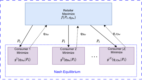
Figure 2: Game-theoretical framework for modeling demand response as a single leader-followers problem. Solid arrows indicate information signals from the retailer, while dashed arrows represent inferences on the consumers behavior.

Thus, the MPEC is expressed as follows:

$$\displaystyle\min_{\bf{X}^{MPEC}} -\sum_{\omega\in{\Omega}}\sigma_{\omega}\left(\sum_{t\in{T},j\in{J}}P_{t}q_{jt\omega}-\sum_{t\in{T}}(P_{t\omega}^{S}q_{t\omega}^{S}+Cy_{t\omega})\right)$$ (5a)

subject to

$$((\ref{1.1}))-((\ref{1.3}))$$ (5b)

$$((\ref{second_1}))-((\ref{second_6}))$$ (5c)

where $\bf{X}^{MPEC}$=$\{P_{t},q_{t\omega}^{S},\delta_{t\omega},y_{t\omega},q_{jt\omega},\Delta_{jt\omega}^{c},\nu_{jt\omega}^{C_{max}},\nu_{jt\omega}^{C_{min}},\varepsilon_{jt\omega},\lambda_{j\omega}\}$ is the set of retailer’s decision variables.

The MPEC optimizes the retailer’s profit subject to its constraints and the KKT optimality conditions of the consumers’ problem. However, the MPEC model in ((5)) has two sources of nonlinearities: (1) the bilinear product $P_{t}q_{jt\omega}$ in the objective function, and (2) the complementarity conditions ((4d))-((4f)) in the consumers’ KKT optimality conditions.

The second type of nonlinearities can be linearized using the strategy proposed in Fortuny-Amat and McCarl (1981), which is by applying the big-M technique. However, we still face the nonlinear product $P_{t}q_{jt\omega}$ which, opposed to other problem settings (Ruiz and Conejo, 2009; Sadat and Fan, 2017) cannot be linearized by employing the strong duality theorem. Hence, we tackle the resulting MPEC with off-the-shelf nonlinear solvers.

3.4 The equilibrium model

Considering perfect competition, we tackle the equilibrium model by the joint solution of retailers and consumers KKT optimality conditions. The resulting system of equations can be linearized and cast as a MILP problem (Fortuny-Amat and McCarl, 1981). In addition, this problem can be addressed directly as a NLP with the same resulting market outcomes (this formulation is included in (A)).

3.4.1 KKT formulation of the retailer problem

The Lagrangian function for the retailer’s problem is:

$$\mathcal{L}(q_{t\omega}^{S},q_{jt\omega})=-\sum_{\omega\in{\Omega},t\in{T},j\in{J}}\sigma_{\omega}P_{t}q_{jt\omega}+\sum_{\omega\in{\Omega},t\in{T}}\Bigl{(}\sigma_{\omega}(P_{t\omega}^{S}q_{t\omega}^{S}+Cy_{t\omega})+\mu_{t\omega}(\delta_{t\omega}+$$

$$-\sum_{t\in{T}}q_{jt\omega}+q_{t\omega}^{S})+\alpha_{t\omega}^{+}(-y_{t\omega}+\delta_{t\omega})+\alpha_{t\omega}^{-}(-y_{t\omega}-\delta_{t\omega})-\theta_{t\omega}q_{t\omega}^{S}-\gamma_{t}P_{t}-\beta_{t\omega}y_{t\omega}\Bigr{)}.$$ (6)

To derive the retailer’s KKT optimality conditions and to deal with the equilibrium model, we assume that the market is in perfect competition, where players compete in terms of deciding their optimal quantities. Thus, $q_{jt\omega}$ also becomes a decision variable for the retailer. This implies that tariff $P_{t}$ is considered exogenous for both retailers’ and consumers’ problems, and its equilibrium value will naturally come out as the market clearing price, i.e., the price that satisfies all the players’ (retailer’s and consumers’) optimality conditions.

The KKT optimality conditions derived from ((3.4.1)) are:

$$\frac{\partial\mathcal{L}}{\partial q_{jt\omega}}=\sigma_{\omega}P_{t}+\mu_{t\omega}=0\quad\forall j,\forall t,\forall\omega$$ (7a)

$$\frac{\partial\mathcal{L}}{\partial q_{t\omega}^{S}}=\mu_{t\omega}+\sigma_{\omega}P_{t\omega}^{S}-\theta_{t\omega}=0\quad\forall t,\forall\omega$$ (7b)

$$\frac{\partial\mathcal{L}}{\partial\delta_{t\omega}}=\mu_{t\omega}+\alpha_{t\omega}^{+}-\alpha_{t\omega}^{-}=0\quad\forall t,\forall\omega$$ (7c)

$$\frac{\partial\mathcal{L}}{\partial y_{t\omega}}=\sigma_{\omega}C-\alpha_{t\omega}^{+}-\alpha_{t\omega}^{-}-\beta_{t\omega}=0\quad\forall t,\forall\omega$$ (7d)

$$\sum_{j\in{J}}q_{jt\omega}-q_{t\omega}^{S}=\delta_{t\omega}\quad\forall t,\forall\omega$$ (7e)

$$0\leq y_{t\omega}-\delta_{t\omega}\perp\alpha_{t\omega}^{+}\geq 0\quad\forall t,\forall\omega$$ (7f)

$$0\leq y_{t\omega}+\delta_{t\omega}\perp\alpha_{t\omega}^{-}\geq 0\quad\forall t,\forall\omega$$ (7g)

$$0\leq q_{t\omega}^{S}\perp\theta_{t\omega}\geq 0\quad\forall t,\forall\omega$$ (7h)

$$0\leq y_{t\omega}\perp\beta_{t\omega}\geq 0\quad\forall t,\forall\omega$$ (7i)

$$\alpha_{t\omega}^{+},\alpha_{t\omega}^{-},\beta_{t\omega},\theta_{t\omega}\geq 0\quad\forall t,\forall\omega$$ (7j)

$$\mu_{t\omega}\quad\text{free}\quad\forall t,\forall\omega.$$ (7k)

3.5 MILP formulation

We solve the equilibrium by concatenating the KKT optimality conditions (((4a))-((4h)) and ((7a))-((7k))). The complementarity slackness conditions ((4d))-((4f)) and ((7f))-((7i)) can be linearized by introducing a binary variable for each condition.

Then to exploit the efficient performance of MILP solvers, the resulting system of MIL constraints can be reformulated as a MILP by including an arbitrary constant as the objective function:

$$\displaystyle\min_{\bf{X}^{Comp}}1$$ (8a)

subject to

$$((\ref{second_1}))-((\ref{cs_1}))$$ (8b)

$$((\ref{second_b}))-((\ref{new_1})),((\ref{new}))$$ (8c)

$$((\ref{lin_4}))-((\ref{lin_5})),((\ref{u_1}))-((\ref{U_2}))\quad\text{and}\quad((\ref{U_3}))-((\ref{U_4}))$$ (8d)

$$\mu_{t\omega}\quad\text{free}\quad\forall t,\forall\omega$$ (8e)

where $\bf{X}^{Comp}$=$\{q_{t\omega}^{S},\delta_{t\omega},y_{t\omega},q_{jt\omega},\Delta_{jt\omega}^{C},\nu_{jt\omega}^{C_{min}},\nu_{jt\omega}^{C_{max}},\varepsilon_{jt\omega},\lambda_{j\omega},\mu_{t\omega},\alpha_{t\omega}^{+},\alpha_{t\omega}^{-},\theta_{t\omega},\beta_{t\omega}\}$ is the set of the decision variables. In particular, the complementarity conditions from the consumer’s KKT conditions can be linearized as follows:

$$\Delta_{jt\omega}^{C}+\Delta_{j}^{C_{max}}\geq 0,\quad\forall j,\forall t,\forall\omega$$ (9a)

$$\Delta_{j}^{C_{max}}-\Delta_{jt\omega}^{C}\geq 0,\quad\forall j,\forall t,\forall\omega$$ (9b)

$$q_{jt\omega}+\Delta_{jt\omega}^{C}\geq 0\quad\forall j,\forall t,\forall\omega$$ (9c)

$$\nu_{jt\omega}^{C_{min}}\geq 0\quad\forall j,\forall t,\forall\omega$$ (9d)

$$\nu_{jt\omega}^{C_{max}}\geq 0\quad\forall j,\forall t,\forall\omega$$ (9e)

$$\varepsilon_{jt\omega}\geq 0\quad\forall j,\forall t,\forall\omega$$ (9f)

$$\Delta_{jt\omega}^{C}+\Delta_{j}^{C_{max}}\leq(1-\psi_{jt\omega}^{C_{min}})M^{c},\quad\forall j,\forall t,\forall\omega$$ (9g)

$$\Delta_{j}^{C_{max}}-\Delta_{jt\omega}^{C}\leq(1-\psi_{jt\omega}^{C_{max}})M^{c},\quad\forall j,\forall t,\forall\omega$$ (9h)

$$q_{jt\omega}+\Delta_{jt\omega}^{C}\leq(1-\psi_{jt\omega})M^{c}\quad\forall j,\forall t,\forall\omega$$ (9i)

$$\nu_{jt\omega}^{C_{min}}\leq\psi_{jt\omega}^{C_{min}}M^{P},\quad\forall j,\forall t,\forall\omega$$ (9j)

$$\nu_{jt\omega}^{C_{max}}\leq\psi_{jt\omega}^{C_{max}}M^{P},\quad\forall j,\forall t,\forall\omega$$ (9k)

$$\varepsilon_{jt\omega}\leq\psi_{jt\omega}M^{P},\quad\forall j,\forall t,\forall\omega$$ (9l)

$$\psi_{jt\omega},\psi_{jt\omega}^{C_{min}},\psi_{jt\omega}^{C_{max}}\in\{0,1\}\quad\forall j,\forall t,\forall\omega$$ (9m)

where $M^{c}$ and $M^{P}$ are large enough constants.

((7f)) and ((7g)) are linearized as follows:

$$y_{t\omega}-\delta_{t\omega}\geq 0,\quad\forall t,\forall\omega$$ (10a)

$$y_{t\omega}+\delta_{t\omega}\geq 0,\quad\forall t,\forall\omega$$ (10b)

$$\alpha_{t\omega}^{+}\geq 0,\quad\forall t,\forall\omega$$ (10c)

$$\alpha_{t\omega}^{-}\geq 0,\quad\forall t,\forall\omega$$ (10d)

$$y_{t\omega}-\delta_{t\omega}\leq(1-\tau_{t\omega}^{+})M^{S}\quad\forall t,\forall\omega$$ (10e)

$$y_{t\omega}+\delta_{t\omega}\leq(1-\tau_{t\omega}^{-})M^{S}\quad\forall t,\forall\omega$$ (10f)

$$\alpha_{t\omega}^{+}\leq\tau_{t\omega}^{+}M^{T},\quad\forall t,\forall\omega$$ (10g)

$$\alpha_{t\omega}^{-}\leq\tau_{t\omega}^{-}M^{T},\quad\forall t,\forall\omega$$ (10h)

$$\tau_{t\omega}^{+},\tau_{t\omega}^{-}\in\{0,1\}$$ (10i)

where $M^{S}$ and $M^{T}$ are large enough constants.

Finally, the linearization of ((7h))-((7k)) renders:

$$q_{t\omega}^{S}\geq 0\quad\forall t,\forall\omega$$ (11a)

$$y_{t\omega}\geq 0\quad\forall t,\forall\omega$$ (11b)

$$\theta_{t\omega}\geq 0\quad\forall t,\forall\omega$$ (11c)

$$\beta_{t\omega}\geq 0\quad\forall t,\forall\omega$$ (11d)

$$q_{t\omega}^{S}\leq(1-\tau_{t\omega}^{q})M^{S},\quad\forall t,\forall\omega$$ (11e)

$$y_{t\omega}\leq(1-\tau_{t\omega}^{y})M^{S},\quad\forall t,\forall\omega$$ (11f)

$$\theta_{t\omega}\leq\tau_{t\omega}^{q}M^{T},\quad\forall t,\forall\omega$$ (11g)

$$\beta_{t\omega}\leq\tau_{t\omega}^{y}M^{T},\quad\forall t,\forall\omega$$ (11h)

$$\tau_{t\omega}^{q},\tau_{t\omega}^{y},\tau_{t}^{P}\in\{0,1\}$$ (11i)

where $M^{S}$ and $M^{T}$ are large enough constants.

4 Numerical results and discussion

In this section we provide numerical examples to complement the analytical results in the previous sections.

4.1 Data and scenario generation

We consider scenarios using an arbitrarily chosen day-ahead electricity spot market prices $P_{t\omega}^{S}$ from the European Energy Exchange market (EEX). These electricity prices are available in one-hour intervals, and we arbitrarily consider the prices on the 20/12/2020, which are available at EEX (2020) along with other market data. We avoid the use of more recent data to exclude distorsions due to the electricity price volatility, caused by geopolitical tensions of recent period.

Therefore, Figure 3 depicts hourly spot market electricity prices and quantities observed on the chosen day where the left axis is the spot price, and the right axis is the spot quantity sold for the corresponding hours. As we discuss in the model formulation part, the marginal utility is the price-demand curve where $A_{jt\omega}$ and $B_{jt\omega}$ are price-demand curve intercept and slope, respectively. Given the data in Figure 3, it is possible to calibrate appropriate expected values for the utility parameters ($A_{jt\omega}$ and $B_{jt\omega}$) and include some perturbations afterwards to consider different levels of residential consumers’ flexibility.

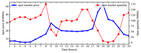
Figure 3: Observed spot price (left axis) and quantity (right axis) sold on EEX with the price on 20 December 2020.

In spite of the fact that there is no theoretical limit on the number of consumers, for simplicity and illustrative purposes, we limit the number of consumers to three. Indeed, this number is sufficient to draw quantitative conclusions on the behavior of the model and the results could be generalized to the average case in reality, at the same time allowing the visualization of relevant variables for each consumer (Zugno et al., 2013). We extend the cases to accommodate different preferences (by varying the demand parameters and demand flexibility) of consumers with respect to consumption shifts. Hence, the expected value of the parameters ($A_{j}$, $B_{j}$ and $\Delta_{j}^{C_{max}}$) are assumed to be slightly different, consumers have different reactions towards the real-time electricity price. For instance, consumer 1 has the lowest slope and the highest flexibility, vice versa for consumer 3, and consumer 2 lies between the two. Since we slightly differentiate demand parameters, consumers act differently in the day-ahead market, which helps us understand the impacts of varying parameters on market outcomes.

Table 1: Parameter mean values considered to represent consumers behavior for different case studies, where $A_{j},B_{j}$ and $\Delta_{j}^{C_{max}}$ are in €/kWh, €/kWh² and kWh, respectively.

	Parameters
Cases	$A_{1}$	$A_{2}$	$A_{3}$	$B_{1}$	$B_{2}$	$B_{3}$	$\Delta_{1}^{C_{max}}$	$\Delta_{2}^{C_{max}}$	$\Delta_{1}^{C_{max}}$
BM	0.0291	0.0302	0.0271	0.0013	0.0015	0.0014	2.50	1.40	2.00
A	0.035	0.0375	0.0341	0.0013	0.0015	0.0014	2.50	1.40	2.00
B	0.0291	0.0302	0.0271	0.0017	0.020	0.0019	2.50	1.40	2.00
Flexibility	0.0291	0.0302	0.0271	0.0013	0.0015	0.0014	5.00	2.40	3.50

We consider a benchmark case (Case BM) and three additional cases obtained by increasing the intercepts $A_{j}$ (Case A), the slopes $B_{j}$ (Case B) and the demand flexibility parameter $\Delta_{j}^{C_{max}}$ (Case flexibility). In other words, the simulation is done by allowing the demand parameters $A_{j}$ to increase while fixing $B_{j}$ and the demand flexibility $\Delta_{j}^{C_{max}}$ at the benchmark and vice versa. In particular, in Case A an increase of 25% with respect to BM for $A_{j}$ is considered, in Case B an increase of 35% for $B_{j}$ and in Case flexibility an increase of 82% from Case BM.

Then, the spot prices for the simulation are randomly generated taking the observed spot market prices as mean values and a coefficient of variation (CV) of 0.015 in a Gaussian process based on the Central Limit Theorem (CLT). The standard deviation is calculated as $CV\times E[P_{t}^{S}]$, which is used to generate $P_{t\omega}^{S}$ with a multivariate normal distribution. Table 1 presents the mean parameter values used for data calibration for the different cases considered in the simulation. The corresponding CVs for $A_{j}$ and $B_{j}$ are 0.013 and 0.0013 so that $A_{jt}\sim N(\mu_{A_{jt}},\sigma_{A_{jt}})$ and $B_{jt}\sim N(\mu_{B_{jt}},\sigma_{B_{jt}})$. Note that we use the same CV (0.013 for $A_{j}$ and 0.0013 for $B_{j}$) for the data calibration in all the cases. The demand flexibility parameter $\Delta_{j}^{C_{max}}$ is arbitrarily allowed to vary from 0 to 5.0kWh, which are reasonable values for individual consumer within DR programs.

The models have been solved using JuMP version 0.21.1 (Dunning et al., 2017) under the open-source Julia programming Language version 1.5.2 (Bezanson et al., 2017). We use Artelys Knitro solver version 12.2 (Artelys Knitro, 2021) for the MPEC and Gurobi version 0.9.12 (Gurobi Optimization, 2021) for the MILP on a CPU E5-1650v2@3.50GHz and 64.00 GB of RAM running workstation. For the MPEC problem we test the case study with $\Omega=30$ equiprobable scenarios and for the competitive market setting $\Omega=300$. It is worth mentioning that increasing the number of scenarios further increases the computational complexity of the MPEC problem, particularly for $\Omega>30$. That is, the number of variables and the number of constraints exponentially increase, which may make the problem computationally intractable. Of course recently, there are possible alternatives to tackle this computational challenge such as by utilizing a supercomputer with parallel computing techniques (we refer the interested reader to Ahmadi-Khatir et al. (2013); Nasri et al. (2015)). In our case, we have employed the option: Knitro multistart in parallel with 12 threads. Moreover, a sensitivity analysis on the number of scenarios shows that, increasing the number of scenarios barely affects the reported market outcomes (Table 2). Note that for the MILP (in the equilibrium), computational burden is not an issue as it could solve for larger sets of scenarios, for example $\Omega=300$ or more. The methods to adjust big Ms are mostly heuristics and problem-dependent, where the trial-and-error procedure has been used in most research works (Motto et al., 2005; Garcés et al., 2009; Jenabi et al., 2013). However, for the particular problem addressed, the tune-up of these constants is achieved without particular numerical trouble. Nevertheless, caution must be exercised in the trial-and-error procedure to ensure that their value is sufficiently large to not impose any additional constraints to the problem, but not too large so that the resulting model is not ill-conditioned (Pineda and Morales, 2019).

Table 2: Sensitivity on number of scenarios in the MPEC model.

	Market outcomes					Market outcomes
$\Omega$	Expected profit	$P_{t}$	$q_{t\omega}^{S}$	$q_{jt\omega}$	$\Omega$	Expected profit	$P_{t}$	$q_{t\omega}^{S}$	$q_{jt\omega}$
10	0.1857	0.0268	14.047	4.682	20	0.1839	0.0267	14.211	4.737
15	0.1850	0.0268	14.074	4.691	30	0.1844	0.02267	14.201	4.733

Table 3: Computational considerations under the two proposed models. Note that MILP is left out of the table because MPEC and NLP are nonlinear models and solved with Knitro while MILP is solved with Gurobi which has a different output summary and not convenient to put together for comparison.

	Number of variables			Number of constraints
Model	bounded below only	free	total	linear equalities	quadratic equalities	linear one-sided inequlities	Total	Number of nonzeros in Jacobian	Number of nonzeros in Hessian	CPU time
MPEC	10,848	5,850	16,698	8,640	6,480	15,864	30,984	118,824	12,984	106.922
NLP	10,848	5,850	16,698	11,520	0	9,360	20,881	120,240	31,680	18.172

Table 3 describes computational performance of the two proposed models and the competitive model performs better (18.172 CPU time) than the model with market power (106.922 CPU time).

4.2 Results of the experiments

In the following, we present simulation results to analyze the market implications of the level of competition and consumers’ flexibility.

4.2.1 Impact on price tariffs

The retailer’s price tariffs in both the MPEC and in the equilibrium models are depicted along with the generated spot market price scenarios for the sake of comparison in Figure 4(a). The four cases considered in the analysis give us the chance to see the impacts of the utility parameters movement and demand flexibility on market outcomes under DR program.

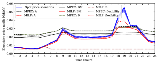
(a) Electricity prices in both models with different cases.

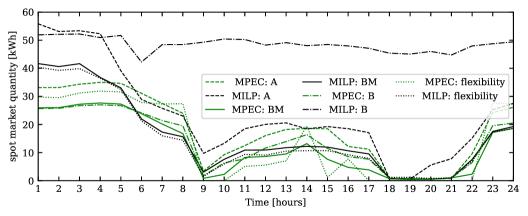
(b) Spot market quantity in both models with different cases.

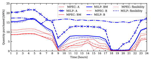
(c) Purchased quantity in both models with different cases.

Figure 4: Electricity price, quantity purchased by the retailer from the spot market and quantity purchased by consumers in the retail market with the two models and with the different cases.

As expected, in the competitive equilibrium model (MILP), price tariffs are apparently lower than the retailer’s tariffs in the MPEC where there is market power. The overall retailer’s price tariffs $P_{t}$ communicated to consumers at time $t$ with the MPEC are proportional and higher than the spot market prices $P_{t\omega}^{S}$, which is economically intuitive. In other words, the retailer tries to decrease its procurement of power at periods $t=9,10,17,18,19,20,21$ where the spot market prices are relatively high, and to increase its purchase at periods $t=1-8,10-17$ where there are lower spot market prices. These price tariff results corroborate with the retailer’s quantities bought in these peak-periods, which are very low, as it can be seen in the spot quantity purchased by retailers (more detail comparison in Figure 10 for the four cases), and higher quantities in the periods where there are lower prices in the wholesale market. Despite the early hours where there are already lower electricity price tariffs, the increase in demand flexibility decreases electricity price tariffs in the MPEC model. However, the increase in both demand parameters ($A$ and $B$) increases price tariffs. Conversely, for the equilibrium model (MILP), only the increase in consumer’s slope $B$ can significantly decrease price tariffs, particularly in peak periods, which is normally expected from consumers’ theory. The overall, price tariff is always below the spot price except the peak periods in the equilibrium model.

The increase in consumers’ flexibility decreases the retailer price tariffs in the MPEC, particularly after 7:00. That means that, if consumers are flexible in their consumption, it is economically meaningful for price to increase and vice versa. However, in the equilibrium, demand flexibility has slightly an opposite impact. Conversely, with the MPEC, the increase in demand flexibility decreases optimal electricity price tariffs. More interestingly, the MPEC model also has the peak-shaving/valley-filling effect; that is, the realized price tariffs at on-peak and off-peak periods are very similar in the case of high flexibility. This is a much-desired result, as a flatter price tariffs curve means that the system is more predictable and reliable.

Figure 4(b) shows electricity procurement in the wholesale market with different cases and models. The retailer buys higher quantities in the perfect competition where there is a lower price, particularly with higher $B$. The retailer’s purchasing trend resembles the observed market trend presented in Figure 3 for all the cases. With the demand flexibility and the BM where there are lower values for $A$ and $\Delta_{j}^{C_{max}}$, the retailer purchases a lower quantity in the equilibrium model. Figure 4(c) shows the aggregate consumers purchase in the retail market with different cases. Since the quantities purchased from the spot market are higher with lower price tariffs, consumers purchase higher quantities in the MILP model irrespective of the case. In the equilibrium model, the increase in $B$ creates higher and stable electricity purchases in the retail market for consumers, which corresponds to the steadily low price-tariffs in this case. With the increase in $A$, for both the MPEC and MILP, consumers buy higher electricity during off-peak periods, otherwise they face higher price tariffs. Because prices in these periods are already low, higher quantities are purchased from the spot market and delivered to the retail market.

From the point of view of a regulator of the market, in case of market power (MPEC), pushing towards flexibility can curb the electricity tariffs especially in the peak hours, even though the quantities purchased are reduced. On the other hand, in case of competitiveness (MILP), high demand elasticity (MILP: B) significantly reduces electricity prices and increases the quantities purchased in both markets.

4.2.2 Impact on retailer’s procurement and consumers’ quantity

As discussed above, Figure 4(b) shows electricity procurement in the wholesale market with different cases and with respect to the two models. The retailer buys higher quantities in the early and late hours of the day-ahead market. With the MILP, and higher $B$, the retailer purchases higher quantities in the spot market, which, in turn, resulted to a lower selling price in the retail market. The higher the competition, the lower is the impact the retailer could have on the market outcomes, which further lowers the selling price back to the consumers. That is why consumers benefit from purchasing their electricity in a competitive equilibrium setting. On the other hand, Figure 4(c) shows the aggregate consumers purchase in the retail market with different cases. As it can be observed, consumers procure much of their electricity consumption in the equilibrium model where there are more quantities and lower price tariffs. Despite the aggregate purchase trend is similar to the individuals purchase, comparing consumers’ purchases in the BM reveals that consumer 1 buys more when electricity price tariffs are low (early morning and late evening see Figure 5). This occurs because in the BM, consumer 1 has the minimum slope (0.0013) and the highest demand flexibility (2.50). Figure 5 shows consumers’ purchase with demand flexibility. Despite that we set $q_{jt\omega}+\Delta_{jt\omega}^{C}\geq 0$ in the model, as it can be seen, Figure 5 depicts negative consumer purchased quantities ($q_{jt\omega}<0$) at some hours, which is realistic in the presence of smart grids where the exchange of energy among prosumers is possible (Li et al., 2011). This implies that, at some hours, using distributed renewable energy, consumers can sell back to the grid their energy surplus.

For example, consumer 3 with the MPEC model and consumer 1 with the MILP model have negative purchase (which implies surplus that can be sold back to the grid) in the high flexibility case.

In addition, since loads are shifted from expensive periods to cheap periods, it can be seen that new peaks and valley periods arise. In other words, if there is a peak period, then the next will be a valley period.

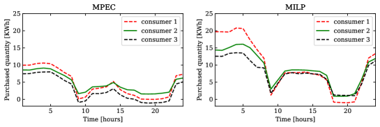
(a) Consumers’ purchase: BM.

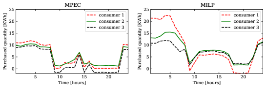
(b) Consumers’ purchase: high flexibility.

Figure 5: Consumers’ purchased quantities in both models with the BM and flexibility cases.

4.2.3 Impact on expected profit

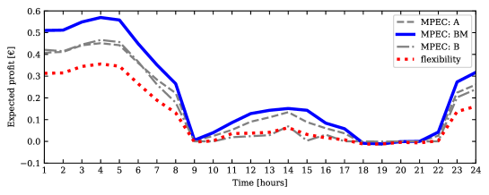
(a) Expected profit for different cases: MPEC.

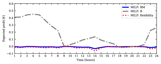
(b) Expected profit for different cases: MILP.

Figure 6: Expected profit comparison between the two models with different cases. Note that MILP: A is not included in this plot as it has negative profits at all time. But we put it in the (B) for comparison purpose.

Looking at the results depicted in Figure 6, which show the expected profit for the retailer in both models, we can observe that the results are directly related to price tariffs and quantities. Since the expected profit for the retailer in the equilibrium model using the increase in $A$ is entirely negative in all periods (not a preferred case for the retailer), we do not include it in the current analysis (see (B)). When market power is exercised (namely in all cases of the MPEC model), the retailer can gain higher expected profits in all time periods. Notice also that in both cases (MPEC and MILP) the retailer may face negative profits in some periods since it maximizes the expected total profit over the entire time horizon (24 hours) and the price tariffs $P_{t}$ at some periods are not necessarily cheaper than the spot market prices $P_{t\omega}^{S}$. However, the retailer faces lower average payoffs with the equilibrium model as the equilibrium price is always below the wholesale market price in all the cases. As opposed to an increase in $A$ where there are monetary losses for the retailer, the increase in parameter $B$ significantly increases the retailer’s profit even with the equilibrium model. With respect to retailer expected profits, we can conclude that in the case of MPEC, higher profits are achieved when $A$ is higher, almost in all time periods, and the expected profits are also higher than the BM. In case of perfect competition, nevertheless, the retailer can achieve higher profits when consumers’ price elasticity is higher.

4.2.4 Consumers’ welfare analysis

(a) Consumers’ welfare for different cases: MPEC.

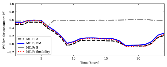
(b) Consumers’ welfare for different cases: MILP.

Figure 7: Consumers’ welfare comparison in the two models with different cases.

In Figure 7 consumer welfare is depicted both for MPEC and MILP models. The welfare results corroborate with other results as consumers obtain higher utility and better welfare in the equilibrium model than the MPEC. For consumers, the equilibrium model provides better welfare as competition decreases price and increases quantity purchases. Therefore, consumers maximize their welfare by shifting their consumption to off-peak periods, which helps to ensure reliable electricity supply during peak periods. This helps to achieve the goal of supply security and reducing price unpredictability, which is the main goal of DR programs.

In addition, since welfare is a direct implication of utility, it increases as demand flexibility increases. This is an insightful result since consumers can increase their welfare by increasing demand flexibility even with the MPEC model where the retailer can obtain higher expected profits. The implication is that the benefits obtained from DR program offsets the cost incurred due to the market power exercised by the retailer.

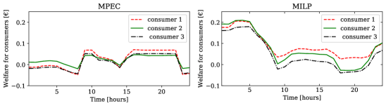
Figure 8: Consumer welfare in both models with respect to the three consumers: BM case where the left plot corresponds to MPEC and the right figure corresponds to the MILP model.

Figure 8 shows individual consumers’ welfare comparison between the two models applying the BM case. All consumers maximize their welfare during off-peak periods in the MILP. For instance, consumer 1 is better off during peak periods as it has higher demand flexibility. On the other hand, consumer 3 has lower welfare in both models due to its lower flexibility. Therefore, it is possible to conclude that welfare is significantly affected by consumers demand flexibility $\Delta_{j}^{C_{max}}$.

Figure 9 shows the pattern of the three consumers’ utility during the 24-hours for the two models. Like their welfare, consumers obtain higher utility during the low-demand periods in the BM case where they incur the least costs. For that reason, consumers shift consumption to off-peak periods because they have lower utility during the peak periods. Overall, the equilibrium provides higher utility, albeit that reverses during peak periods.

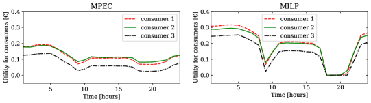
Figure 9: Consumers’ utility in both models: BM case.

4.2.5 DR effectiveness: further comparisons

In this Section we draw some further insight from our analysis by deepening on the comparisons between price tariffs, quantities and demand flexibility.

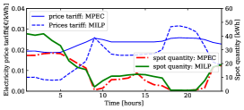
(a) Price-quantity comparison: BM.

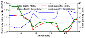
(b) Price-quantity comparison: A.

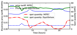
(c) Price-quantity comparison: B.

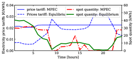
(d) Price-quantity comparison: flexibility.

Figure 10: Price (left axis) and spot quantity (right axis) comparison in both models and for the four cases. Note also the legends for panel (b), (c) and (d) are as expressed in panel (a).

Figure 10 presents price tariffs and quantities purchased by the retailer from the spot market in both models. For the sake of comparison, we plot price tariffs on the left axis and spot market quantity on the right axis so that it is possible to analyze the impact of parameter changes on the spot market purchase and price tariffs. As discussed before, price tariffs, particularly with the MILP, decrease when demand flexibility increases. However, the increase in $A$ increases price tariffs, whereas the increase in $B$ decreases price, which is in line with the economic theory of demand. For that reason, the retailer buys a higher spot quantity from the wholesale market if he expects that $B$ increases.

In general, electricity price tariffs set by the retailer and spot market quantity follow a similar trend to the observed real market trend and the consumers’ procurement, which we discussed before. Thus, the models fully characterize the market participants’ (the retailer’s and consumers’) behaviors so that policy implications can be drawn from the the proposed model. Consumers are better off purchasing their electricity consumption with the equilibrium model as it has a lower price than the MPEC model. However, the retailer benefits from the MPEC model as it gives the retailer a higher expected profit, which is its primary objective. In addition, despite prices are relatively stable in the MPEC model, the quantities purchased in the spot market are highly affected by the variation of demand parameters. In particular, with flexibility is (subplot d) in Figure 10) spot quantities follow a different pattern.

Concerning the MILP model, high elasticity of the demand (case B) increases the quantities purchased in the spot market in all periods due to the lower price. This behavior does not occur in the other cases. The main implication of this analysis, from a regulator point of view is that, depending on the market structure, trying to act on the different parameters can modify the choices on spot market decisions.

Figure 11 depicts results regarding consumers’ flexibility (DR) towards their consumption for the two models with the BM and with higher flexibility. The overall trend for flexible demand is almost similar in both models, though differences in magnitudes. Consumers are more flexible from 9:00-11:00 and from 17:00-22:00 as they shift their consumption to the off-peak periods. In relation to this, the negative values show consumers shift part of their consumption in those hours as they consume higher energy in the off-peak periods. The result also guarantees the constraint $\sum_{t\in{T}}\Delta_{jt\omega}^{C}=0$, and the flexibility boundary values given for each consumers in Table 1. For instance, consumer 1 is with higher flexibility in consumption up to 5kWh compared to the other consumers. For the case where we have more flexibility, the overall electricity price is decreased, and the quantity purchased is increased. As a result, the results on the retailer’s profit and consumers’ welfare are robust. Thus, the DR models effectively characterize the market in both market configurations.

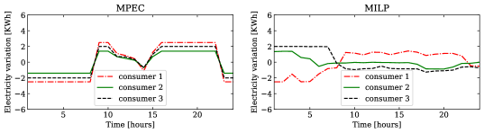
(a) Level of flexibility for consumers: BM.

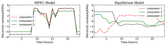
(b) Level of flexibility for consumers: high flexibility.

Figure 11: Variation of demand in both models with respect to the two cases.

4.2.6 Market performance and sensitivity analysis

Table 4: Market performance of retailer and consumers in the simulations (with the benchmark case). Note all the values but price (€/kWh) are averages for the considered scenarios ($\Omega=30$) and expressed in €.

Retailer	Model		Consumers	Model
Performance index	MPEC	Equilibrium	performance index	MPEC	Equilibrium
Expected profit	0.1149	-0.0076	Cost	0.2602	0.2894
Revenue	0.2602	0.2894	Price	0.0230	0.0177
Cost	0.1454	0.2970	Welfare	0.0177	0.0784

Table 4 presents the performance of the two models for the retailer and consumers where values are measured on average under the BM case. As the expected profit reveals, the retailer loses money on average in the equilibrium despite that consumers enjoy better welfare from their consumption with lower prices. Note that cost for the retailer comes of two sources: the spot market purchasing costs if the retailer had perfect information from future consumption and the imbalance penalties, which are the costs of imperfect information. Furthermore, note that the retailer’s revenue is a cost for the consumers.

Table 5: Sensitivity analysis on spot price uncertainty under the MPEC model for the BM case.

Spot price uncertainty	Exp. profit	Max. profit	Min. profit	$q_{t\omega}$	$q_{jt\omega}$	Tariff	Utility	Welfare
0.015	0.1143	0.3555	-0.0128	12.29	4.198	0.0230	0.1046	0.0177
0.030	0.1156	0.3551	-0.0140	12.30	4.101	0.0230	0.1046	0.0177
0.035	0.1156	0.3547	-0.0141	12.31	4.105	0.0230	0.1047	0.0178

In Table 5, we present the market outcomes regarding the uncertainty of the spot market prices $P_{t\omega}^{S}$ under the BM case and the MPEC model. We consider the coefficient of variations for this analysis to be only 0.015, 0.003, and 0.035 for the sake of simplicity. The results show that the uncertainty on the spot market price has no significant impact on market outcomes for both the retailer and end-consumers. Instead, as proved through the simulation, the level of demand flexibility affects the market outcomes significantly. This means that demand flexibility is able to reduce the impact of spot market uncertainties could have on market outcomes.

5 Conclusions

This paper presents two game-theoretical models for a retailer and consumers participating in the electricity market under demand response. Our research complements prior works on demand response by considering the flexibility of consumers under dynamic price tariffs and characterizing their behavior using a utility function. We consider welfare-maximizing consumers that interact in the retail market in a leader-follower or in a perfect competition market configuration. The first case is modeled with a bilevel optimization problem. In the lower level, a dynamic model with responsive demand based on realistic consumers’ preferences is explicitly formulated using a quadratic utility function. This leader-followers game is solved as a nonlinear MPEC where a retailer with market power selects an optimal tariff taking into account the behavior of the consumers, which can react to these selling prices by modifying their consumption profiles. We also explore the equilibrium model with perfect competition which is solved as a MILP problem.

The dynamic pricing DR program has been shown to effectively shift electricity demand if there are incentives for both retailers and consumers to participate in the program. The results allow the retailer to optimize its pricing strategy with market power (MPEC), and the consumers to maximize their welfare in a competitive equilibrium setting. The numerical results further demonstrate that the proposed models are adaptable to any group of consumers with participation in DR programs and can be adjusted for any period according to the preferences given by consumers. For both models, consumers are flexible enough to exercise the DR program. We discuss the impact of demand parameters and demand-side flexibility on market outcomes in detail with different case studies. The results attest that including consumers’ utility function in a DR program explicitly, reveals important features of consumers’ behavior. Finally, through a sensitivity analysis and under spot price uncertainty, it is shown that there is an economic incentive for consumers to increase their flexibility, which, in turn, benefits the retailer as well.

Finally, our proposed procedures are able to give the following managerial and economic insights: (i) they attempt to handle both demand-side and supply-side uncertainties by proposing stochastic programming from a methodological perspective, (ii) they highlight which market configuration is best for each market participant having the options to allow for greater flexibility of price-tariffs/loads negotiations between consumers and retailers, and (iii) they bring a significant effect on cost savings and improved economic efficiency in power systems.

The comparison between the different market structures (market power in MPEC and competition in MILP) as well as the sensitivity analysis in the demand parameters can pursue the regulator of the market to incentivize flexibility or to enhance elasticity of the demand to maximize the social welfare, reduce the price and the volatility of the quantities purchased in the different markets in both market configurations.

The proposed game-theoretical optimization model can be further extended in different directions. First, we can model generating companies and market operators’ problems with a DR program by applying a similar methodology employed in this paper. Second, within the same model and players, we can include RES generation and grid constraints by explicitly modeling consumers’ problems with intelligent appliances so that they can trade their energy each other instead of being net consumers. Third, since only a few works address on environmental effects of DR programs, we can consider pollution in the objective function of the DR optimization problem which could give better policy directions to the integration of technology, market, and innovation in the power system to achieve emission reduction and economic efficiency with a reduced social cost.

Appendix A NLP formulation

The equilibrium problem described in Section (3.4), can also be addressed in terms of a nonlinear optimization problem by minimizing the sum of the complementarity conditions in ((7)) subject to the rest of equality and inequality KKT constraints, as proposed by Leyffer and Munson (2010) applied for similar reformulation of NLP by Abate et al. (2022).

$$\displaystyle\min\sum_{\omega\in{\Omega},t\in{T},j\in{J}}\{\nu_{jt\omega}^{C_{min}}(\Delta_{jt\omega}^{C}+\Delta_{j}^{C_{max}})+\nu_{jt\omega}^{C_{max}}(\Delta_{j}^{C_{max}}-\Delta_{jt\omega}^{C})+\varepsilon_{jt\omega}(q_{jt\omega}+\Delta_{jt\omega}^{C})\}+$$

$$+\sum_{\omega\in{\Omega},t\in{T}}\{\alpha_{t\omega}^{+}(y_{t\omega}-\delta_{t\omega})+\alpha_{t\omega}^{-}(y_{t\omega}+\delta_{t\omega})+y_{t\omega}\beta_{t\omega}+q_{t\omega}^{S}\theta_{t\omega}\}$$ (12a)

subject to

$$((\ref{second_1}))-((\ref{cs_1}))$$ (12b)

$$((\ref{second_b}))-((\ref{new_1}))$$ (12c)

$$\Delta_{jt\omega}^{C}+\Delta_{j}^{C_{max}}\geq 0\quad\forall j,\forall t,\forall\omega$$ (12d)

$$q_{jt\omega}+\Delta_{jt\omega}^{C}\geq 0\quad\forall j,\forall t,\forall\omega$$ (12e)

$$\Delta_{j}^{C_{max}}-\Delta_{jt\omega}^{C}\geq 0\quad\forall j,\forall t,\forall\omega$$ (12f)

$$y_{t\omega}-\delta_{t\omega}\geq 0\quad\forall t,\forall\omega$$ (12g)

$$y_{t\omega}+\delta_{t\omega}\geq 0\quad\forall t,\forall\omega$$ (12h)

$$q_{t\omega}^{S}\geq 0\quad\forall t,\forall\omega$$ (12i)

$$y_{t\omega}\geq 0\quad\forall t,\forall\omega$$ (12j)

$$\alpha_{t\omega}^{+},\alpha_{t\omega}^{-},\beta_{t\omega},\varepsilon_{jt\omega},\theta_{t\omega},\nu_{jt\omega}^{C_{min}},\nu_{jt\omega}^{C_{max}}\geq 0\quad\forall j,\forall t,\forall\omega$$ (12k)

$$\lambda_{j\omega},\mu_{t\omega}\quad\forall j,\forall t,\forall\omega\quad\text{free.}$$ (12l)

Note that, if at the optimal solution the objective function ((12a)) is 0, then each of its (non-negative) terms must be zero too, which guarantees the satisfaction of the original complementarity constraints, together with the rest of KKT conditions. This characterizes a candidate solution of the retailer-consumer equilibrium.

Appendix B Some additional results

For completeness, in Figure 12, we depict the expected profit results using the increase in parameter A for the MILP model. As we can see, the expected profit is entirely negative. That means the retailer may participate in the DR program to avoid a higher penalty in this case. On the other hand, as the increase in parameter A decreases price tariffs, it is unavoidable to have expected negative profits.

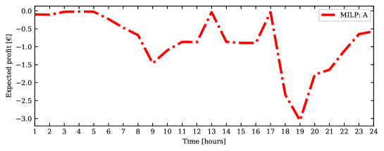
Figure 12: Expected profit in the equilibrium model (MILP: A).

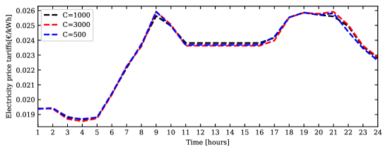
Figure 13: Price tariffs with the MPEC model using the BM for different values of penalty (500, 1000, 3000).

Although it affects the power imbalance at a specific time, penalizing the retailer’s objective function with weight $C$ has no significant effect on the market outcomes. For instance, Figure 13 shows the price tariffs using the BM ($C=500$, $C=1000$ and $C=3000$). The three price tariff curves seem to be indifferent throughout the period. However, a higher imbalance penalty may result in negative expected profits.

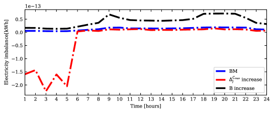
Figure 14: Electricity imbalances for different cases in the MPEC model.

Figure 14 shows the electricity imbalance $\delta_{t\omega}$ with the BM, and by increasing $B$ and $\Delta_{j}^{C_{max}}$. When demand flexibility increases, $\delta_{t\omega}$ becomes negative in the off-peak periods, which economically makes sense as consumers shift their consumption to these periods and that can create negative imbalance from the retailer side. The opposite can happen when $B$ increases.

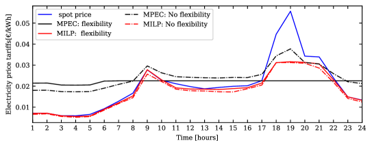
Figure 15: Electricity prices comparison in both models considering non flexible demand and the BM.

To complement the analysis, we compare prices with and without demand flexibility in Figure 15 for the MPEC and the MILP models. Without demand flexibility, price tariffs are higher in the BM under the MPEC model than for the equilibrium model (MILP). Since prices does not significantly change over time in the BM case, we compare them with a higher flexibility, which resulted in higher prices. This is a counterintuitive result that indicates price tariffs increase if consumer demand flexibility increases, which may be due to the nature of the competition since prices are already below the spot market prices under the BM case.

References

- Abate et al. (2021) Abate, A. G., Riccardi, R., and Ruiz, C. (2021). Contracts in electricity markets under eu ets: A stochastic programming approach. Energy Economics, page 105309.
- Abate et al. (2022) Abate, A. G., Riccardi, R., and Ruiz, C. (2022). Contract design in electricity markets with high penetration of renewables: A two-stage approach. Omega, 111:102666.
- Afşar et al. (2016) Afşar, S., Brotcorne, L., Marcotte, P., and Savard, G. (2016). Achieving an optimal trade-off between revenue and energy peak within a smart grid environment. Renewable Energy, 91:293–301.
- Ahmadi-Khatir et al. (2013) Ahmadi-Khatir, A., Conejo, A. J., and Cherkaoui, R. (2013). Multi-area unit scheduling and reserve allocation under wind power uncertainty. IEEE Transactions on power systems, 29(4):1701–1710.
- Ajoulabadi et al. (2020) Ajoulabadi, A., Ravadanegh, S. N., and Mohammadi-Ivatloo, B. (2020). Flexible scheduling of reconfigurable microgrid-based distribution networks considering demand response program. Energy, 196:117024.
- Alipour et al. (2019) Alipour, M., Zare, K., Seyedi, H., and Jalali, M. (2019). Real-time price-based demand response model for combined heat and power systems. Energy, 168:1119–1127.
- Antunes et al. (2020) Antunes, C. H., Alves, M. J., and Ecer, B. (2020). Bilevel optimization to deal with demand response in power grids: models, methods and challenges. TOP, pages 1–29.
- Artelys Knitro (2021) Artelys Knitro, L. (2021). The artelys knitro user’s manual.
- Askeland et al. (2020) Askeland, M., Burandt, T., and Gabriel, S. A. (2020). A stochastic mpec approach for grid tariff design with demand-side flexibility. Energy Systems, pages 1–23.
- Aussel et al. (2020) Aussel, D., Brotcorne, L., Lepaul, S., and von Niederhäusern, L. (2020). A trilevel model for best response in energy demand-side management. European Journal of Operational Research, 281(2):299–315.
- Bezanson et al. (2017) Bezanson, J., Edelman, A., Karpinski, S., and Shah, V. B. (2017). Julia: A fresh approach to numerical computing. SIAM Review, 59(1):65–98.
- Chen et al. (2010) Chen, L., Li, N., Low, S. H., and Doyle, J. C. (2010). Two market models for demand response in power networks. In 2010 First IEEE International Conference on Smart Grid Communications, pages 397–402. IEEE.
- Cicek and Delic (2015) Cicek, N. and Delic, H. (2015). Demand response management for smart grids with wind power. IEEE Transactions on Sustainable Energy, 6(2):625–634.
- Corradi et al. (2012) Corradi, O., Ochsenfeld, H., Madsen, H., and Pinson, P. (2012). Controlling electricity consumption by forecasting its response to varying prices. IEEE Transactions on Power Systems, 28(1):421–429.
- Dagoumas and Polemis (2017) Dagoumas, A. S. and Polemis, M. L. (2017). An integrated model for assessing electricity retailer’s profitability with demand response. Applied Energy, 198:49–64.
- Daraeepour et al. (2015) Daraeepour, A., Kazempour, S. J., Patiño-Echeverri, D., and Conejo, A. J. (2015). Strategic demand-side response to wind power integration. IEEE Transactions on Power Systems, 31(5):3495–3505.
- Dunning et al. (2017) Dunning, I., Huchette, J., and Lubin, M. (2017). Jump: A modeling language for mathematical optimization. SIAM Review, 59(2):295–320.
- Dvorkin (2017) Dvorkin, Y. (2017). Can merchant demand response affect investments in merchant energy storage? IEEE Transactions on Power Systems, 33(3):2671–2683.
- EEX (2020) EEX (2020). Market Data, European Emission Allowances Futures.
- Fan (2012) Fan, Z. (2012). A distributed demand response algorithm and its application to phev charging in smart grids. IEEE Transactions on Smart Grid, 3(3):1280–1290.
- Fortuny-Amat and McCarl (1981) Fortuny-Amat, J. and McCarl, B. (1981). A representation and economic interpretation of a two-level programming problem. Journal of the Operational Research Society, 32(9):783–792.
- Garcés et al. (2009) Garcés, L. P., Conejo, A. J., García-Bertrand, R., and Romero, R. (2009). A bilevel approach to transmission expansion planning within a market environment. IEEE Transactions on Power Systems, 24(3):1513–1522.
- Guo and Weeks (2022) Guo, B. and Weeks, M. (2022). Dynamic tariffs, demand response, and regulation in retail electricity markets. Energy Economics, 106:105774.
- Gurobi Optimization (2021) Gurobi Optimization, L. (2021). Gurobi optimizer reference manual.
- Haghighat and Kennedy (2012) Haghighat, H. and Kennedy, S. W. (2012). A bilevel approach to operational decision making of a distribution company in competitive environments. IEEE Transactions on Power Systems, 27(4):1797–1807.
- Hakimi et al. (2019) Hakimi, S. M., Hasankhani, A., Shafie-khah, M., and Catalão, J. P. (2019). Optimal sizing and siting of smart microgrid components under high renewables penetration considering demand response. IET Renewable power generation, 13(10):1809–1822.
- Halvgaard et al. (2012) Halvgaard, R., Poulsen, N. K., Madsen, H., and Jørgensen, J. B. (2012). Economic model predictive control for building climate control in a smart grid. In 2012 IEEE PES Innovative Smart Grid Technologies (ISGT), pages 1–6. IEEE.
- He et al. (2013) He, X., Keyaerts, N., Azevedo, I., Meeus, L., Hancher, L., and Glachant, J.-M. (2013). How to engage consumers in demand response: A contract perspective. Utilities Policy, 27:108–122.
- Hu et al. (2016) Hu, M.-C., Lu, S.-Y., and Chen, Y.-H. (2016). Stochastic–multiobjective market equilibrium analysis of a demand response program in energy market under uncertainty. Applied Energy, 182:500–506.
- Ilic et al. (2011) Ilic, M. D., Xie, L., and Joo, J.-Y. (2011). Efficient coordination of wind power and price-responsive demand—part i: Theoretical foundations. IEEE Transactions on Power Systems, 26(4):1875–1884.
- Jenabi et al. (2013) Jenabi, M., Ghomi, S. M. T. F., and Smeers, Y. (2013). Bi-level game approaches for coordination of generation and transmission expansion planning within a market environment. IEEE Transactions on Power systems, 28(3):2639–2650.
- Leyffer and Munson (2010) Leyffer, S. and Munson, T. (2010). Solving multi-leader–common-follower games. Optimisation Methods & Software, 25(4):601–623.
- Li et al. (2011) Li, N., Chen, L., and Low, S. H. (2011). Optimal demand response based on utility maximization in power networks. In 2011 IEEE power and energy society general meeting, pages 1–8. IEEE.
- Li et al. (2015) Li, Z., Shahidehpour, M., Alabdulwahab, A., and Abusorrah, A. (2015). Bilevel model for analyzing coordinated cyber-physical attacks on power systems. IEEE Transactions on Smart Grid, 7(5):2260–2272.
- Lu et al. (2018) Lu, R., Hong, S. H., and Zhang, X. (2018). A dynamic pricing demand response algorithm for smart grid: reinforcement learning approach. Applied Energy, 220:220–230.
- Luo et al. (2020) Luo, X., Liu, Y., Liu, J., and Liu, X. (2020). Energy scheduling for a three-level integrated energy system based on energy hub models: A hierarchical stackelberg game approach. Sustainable Cities and Society, 52:101814.
- Luo et al. (1996) Luo, Z.-Q., Pang, J.-S., and Ralph, D. (1996). Mathematical programs with equilibrium constraints. Cambridge University Press.
- Ma et al. (2014) Ma, K., Hu, G., and Spanos, C. J. (2014). Dynamics of electricity markets with unknown utility functions: An extremum seeking control approach. In 11th IEEE International Conference on Control & Automation (ICCA), pages 302–307. IEEE.
- Mohsenian-Rad et al. (2010) Mohsenian-Rad, A.-H., Wong, V. W., Jatskevich, J., Schober, R., and Leon-Garcia, A. (2010). Autonomous demand-side management based on game-theoretic energy consumption scheduling for the future smart grid. IEEE transactions on Smart Grid, 1(3):320–331.
- Momber et al. (2015) Momber, I., Wogrin, S., and San Román, T. G. (2015). Retail pricing: A bilevel program for pev aggregator decisions using indirect load control. IEEE Transactions on Power Systems, 31(1):464–473.
- Morales et al. (2013) Morales, J. M., Conejo, A. J., Madsen, H., Pinson, P., and Zugno, M. (2013). Integrating renewables in electricity markets: operational problems, volume 205. Springer Science & Business Media.
- Morales-España et al. (2021) Morales-España, G., Nycander, E., and Sijm, J. (2021). Reducing co2 emissions by curtailing renewables: Examples from optimal power system operation. Energy Economics, 99:105277.
- Motto et al. (2005) Motto, A. L., Arroyo, J. M., and Galiana, F. D. (2005). A mixed-integer lp procedure for the analysis of electric grid security under disruptive threat. IEEE Transactions on Power Systems, 20(3):1357–1365.
- Nasri et al. (2015) Nasri, A., Kazempour, S. J., Conejo, A. J., and Ghandhari, M. (2015). Network-constrained ac unit commitment under uncertainty: a benders’ decomposition approach. IEEE transactions on power systems, 31(1):412–422.
- Nasrolahpour et al. (2016) Nasrolahpour, E., Kazempour, S. J., Zareipour, H., and Rosehart, W. D. (2016). Strategic sizing of energy storage facilities in electricity markets. IEEE Transactions on Sustainable Energy, 7(4):1462–1472.
- Nejad et al. (2019) Nejad, H. C., Tavakoli, S., Ghadimi, N., Korjani, S., Nojavan, S., and Pashaei-Didani, H. (2019). Reliability based optimal allocation of distributed generations in transmission systems under demand response program. Electric Power Systems Research, 176:105952.
- Nguyen et al. (2016) Nguyen, D. T., Nguyen, H. T., and Le, L. B. (2016). Dynamic pricing design for demand response integration in power distribution networks. IEEE Transactions on Power Systems, 31(5):3457–3472.
- Nilsson et al. (2018) Nilsson, A., Lazarevic, D., Brandt, N., and Kordas, O. (2018). Household responsiveness to residential demand response strategies: Results and policy implications from a swedish field study. Energy policy, 122:273–286.
- Niromandfam et al. (2020) Niromandfam, A., Yazdankhah, A. S., and Kazemzadeh, R. (2020). Modeling demand response based on utility function considering wind profit maximization in the day-ahead market. Journal of Cleaner Production, 251:119317.
- Nolan and O’Malley (2015) Nolan, S. and O’Malley, M. (2015). Challenges and barriers to demand response deployment and evaluation. Applied Energy, 152:1–10.
- Pallonetto et al. (2020) Pallonetto, F., De Rosa, M., D’Ettorre, F., and Finn, D. P. (2020). On the assessment and control optimisation of demand response programs in residential buildings. Renewable and Sustainable Energy Reviews, 127:109861.
- Parvania et al. (2013) Parvania, M., Fotuhi-Firuzabad, M., and Shahidehpour, M. (2013). Optimal demand response aggregation in wholesale electricity markets. IEEE Transactions on Smart Grid, 4(4):1957–1965.
- Pineda and Morales (2019) Pineda, S. and Morales, J. M. (2019). Solving linear bilevel problems using big-ms: not all that glitters is gold. IEEE Transactions on Power Systems, 34(3):2469–2471.
- Rubinstein et al. (2006) Rubinstein, A. et al. (2006). Lecture notes in microeconomic theory. Princeton, NJ: Princeton University.
- Ruiz and Conejo (2009) Ruiz, C. and Conejo, A. J. (2009). Pool strategy of a producer with endogenous formation of locational marginal prices. IEEE Transactions on Power Systems, 24(4):1855–1866.
- Ruiz et al. (2018) Ruiz, C., Nogales, F., and Prieto, F. (2018). Retail equilibrium with switching consumers in electricity markets. Networks and Spatial Economics, 18(1):145–180.
- Sadat and Fan (2017) Sadat, S. A. and Fan, L. (2017). Mixed integer linear programming formulation for chance constrained mathematical programs with equilibrium constraints. In 2017 IEEE Power & Energy Society General Meeting, pages 1–5. IEEE.
- Samadi et al. (2010) Samadi, P., Mohsenian-Rad, A.-H., Schober, R., Wong, V. W., and Jatskevich, J. (2010). Optimal real-time pricing algorithm based on utility maximization for smart grid. In 2010 First IEEE International Conference on Smart Grid Communications, pages 415–420. IEEE.
- Setlhaolo et al. (2014) Setlhaolo, D., Xia, X., and Zhang, J. (2014). Optimal scheduling of household appliances for demand response. Electric Power Systems Research, 116:24–28.
- Sharifi et al. (2017) Sharifi, R., Anvari-Moghaddam, A., Fathi, S. H., Guerrero, J. M., and Vahidinasab, V. (2017). Economic demand response model in liberalised electricity markets with respect to flexibility of consumers. IET Generation, Transmission & Distribution, 11(17):4291–4298.
- Shen et al. (2014) Shen, B., Ghatikar, G., Lei, Z., Li, J., Wikler, G., and Martin, P. (2014). The role of regulatory reforms, market changes, and technology development to make demand response a viable resource in meeting energy challenges. Applied Energy, 130:814–823.
- Soares et al. (2020) Soares, I., Alves, M. J., and Antunes, C. H. (2020). Designing time-of-use tariffs in electricity retail markets using a bi-level model–estimating bounds when the lower level problem cannot be exactly solved. Omega, 93:102027.
- Soares et al. (2019) Soares, I., Alves, M. J., and Henggeler Antunes, C. (2019). A population-based approach to the bi-level multifollower problem: an application to the electricity retail market. International Transactions in Operational Research.
- Vayá and Andersson (2014) Vayá, M. G. and Andersson, G. (2014). Optimal bidding strategy of a plug-in electric vehicle aggregator in day-ahead electricity markets under uncertainty. IEEE Transactions on Power Systems, 30(5):2375–2385.
- Von Stackelberg (2010) Von Stackelberg, H. (2010). Market structure and equilibrium. Springer Science & Business Media.
- Wang et al. (2020a) Wang, F., Xiang, B., Li, K., Ge, X., Lu, H., Lai, J., and Dehghanian, P. (2020a). Smart households’ aggregated capacity forecasting for load aggregators under incentive-based demand response programs. IEEE Transactions on Industry Applications, 56(2):1086–1097.
- Wang et al. (2020b) Wang, Y., Ma, Y., Song, F., Ma, Y., Qi, C., Huang, F., Xing, J., and Zhang, F. (2020b). Economic and efficient multi-objective operation optimization of integrated energy system considering electro-thermal demand response. Energy, 205:118022.
- Wu et al. (2015) Wu, H., Shahidehpour, M., Alabdulwahab, A., and Abusorrah, A. (2015). Demand response exchange in the stochastic day-ahead scheduling with variable renewable generation. IEEE Transactions on Sustainable Energy, 6(2):516–525.
- Zugno et al. (2013) Zugno, M., Morales, J. M., Pinson, P., and Madsen, H. (2013). A bilevel model for electricity retailers’ participation in a demand response market environment. Energy Economics, 36:182–197.