Model-based Multi-agent Policy Optimization
with Adaptive Opponent-wise Rollouts

Abstract

This paper investigates the model-based methods in multi-agent reinforcement learning (MARL). We specify the dynamics sample complexity and the opponent sample complexity in MARL, and conduct a theoretic analysis of return discrepancy upper bound. To reduce the upper bound with the intention of low sample complexity during the whole learning process, we propose a novel decentralized model-based MARL method, named Adaptive Opponent-wise Rollout Policy Optimization (AORPO). In AORPO, each agent builds its multi-agent environment model, consisting of a dynamics model and multiple opponent models, and trains its policy with the adaptive opponent-wise rollout. We further prove the theoretic convergence of AORPO under reasonable assumptions. Empirical experiments on competitive and cooperative tasks demonstrate that AORPO can achieve improved sample efficiency with comparable asymptotic performance over the compared MARL methods.

1 Introduction

Multi-agent reinforcement learning (MARL) has been recently paid much attention and preliminarily applied to various control scenarios including robot system, autonomous driving, resource utilization etc. Du and Ding (2020). One main technical challenge MARL brings over single-agent reinforcement learning (SARL) is that the agents need to interact with other agents, and their returns depend on the behavior of all the agents, which usually requires a considerable amount of samples, i.e., high sample complexity.

In a general MARL setting, one agent can access the actions taken by other agents in any state through some communication protocol, without any knowledge of their specific policies Tian et al. (2020). In such a situation, we claim that the sample complexity in MARL comes from two parts: dynamics sample complexity and opponent sample complexity. To achieve some policy performance, dynamics sample complexity represents the number of interactions made with the environment dynamics while collecting the samples. On the other hand, opponent sample complexity, which is unique in MARL, represents the times of communications to access one opponent’s action. Thus one goal of MARL is to find an effective policy with the two sample complexities being low.

In SARL scenarios, it is well known that model-based reinforcement learning (MBRL) can achieve lower dynamics sample complexity than model-free reinforcement learning (MFRL) empirically Wang et al. (2019) or achieve at least competitive complexity theoretically Jin et al. (2018). Specifically, by building a dynamics model, the agent can also be trained with the model simulation samples and the ones collected from the environment, which can reduce the need for the environment samples Luo et al. (2019). In multi-agent scenarios, however, to utilize the dynamics model for data simulation, we need to ask for the opponents’ actions through a communication protocol, which will count as the opponent sample complexity. Via building opponent models He et al. (2016), we can replace the real opponents in the data simulation stage to reduce the opponent sample complexity.

In this paper, we investigate model-based methods for MARL and propose a novel method called Adaptive Opponent-wise Rollout Policy Optimization (AORPO). Specifically, from the perspective of each ego agent, we build a multi-agent environment model, which consists of a dynamics model and opponent models for each opponent agent. The multi-agent environment model can then be used to perform simulation rollout for MARL training to reduce both sample complexities. To our knowledge, however, in literature, there is no theoretical guidance regarding how to perform the multi-agent simulated rollouts. We provide a theoretical analysis about the upper bound of the return discrepancy w.r.t. policy distribution shift and the generalization errors of the environment dynamics and each opponent model. The upper bound reveals that when the environment dynamics model performs rollout with multiple opponents models, different magnitudes of opponent model errors may lead to different contributions to the compounding error of the multi-step simulated rollouts. Based on the theoretic analysis, we design the adaptive opponent-wise rollout scheme for our policy optimization algorithm, called AORPO, and prove its convergence under reasonable assumptions.

Experiments show that AORPO outperforms several state-of-the-art MARL methods in terms of sample efficiency in both cooperative tasks and competitive tasks.

2 Related Work

There are two important training paradigms in MARL, i.e., centralized training with decentralized execution (CTDE) and fully decentralized training. Typical algorithms using CTDE paradigm are value function decomposition algorithms Whiteson (2018), which deal with the non-stationarity and credit-assignment challenges by a centralized value function. Fully decentralized MARL algorithms include consensus learning over networked agents and communicating agents Zhang et al. (2018); Qu et al. (2019). In decentralized scenarios, where the agents can communicate with each other, Iqbal and Sha Iqbal and Sha (2019) proposed a method that integrates the received messages to learn a value function and a policy. In this paper, we propose a fully decentralized training method with a communication protocol.

Opponent modeling He et al. (2016) is a feasible solution to the non-stationarity problem in MARL, which models others’ policies with interaction experience. Behavior cloning is a straightforward method to learn opponents’ policies Lowe et al. (2017). More advances include recursive reasoning with variational inference Wen et al. (2019), maximum-entropy objective Tian et al. (2019), and modeling the learning process of opponents Foerster et al. (2018) etc.

There are generally two major problems for model-based RL methods, i.e., model learning and model usage. For model learning, the most common solution is supervised learning Nagabandi et al. (2018), or non-parametric methods such as Gaussian processes Kamthe and Deisenroth (2018). For model usage, a policy can be derived by exploiting the model with different algorithms such as Dyna Sutton (1990), shooting methods Chua et al. (2018) and policy search with backpropagation through paths Clavera et al. (2020). We refer to Wang et al. Wang et al. (2019) for details of model-based RL. Theoretical analysis of model-based RL in single-agent scenarios has been investigated in recent literature. To name a few, Luo et al. Luo et al. (2019) provided a monotonic improvement guarantee by enforcing a distance constraint between the learning policy and the data-collecting policy. Janner et al. Janner et al. (2019) derived a return discrepancy bound with the branched rollout, which studies how the model generalization affects the model usage.

For model-based MARL, there are relatively limited works of literature, to our knowledge. Park et al. Park et al. (2019) proposed to use a centralized auxiliary prediction network to model the environment dynamics to alleviate the non-stationary dynamics problem. Kamra et al. Kamra et al. (2020) and Li et al. Li et al. (2020) proposed interaction graph-based trajectory prediction methods, without considering policies. Krupnik et al. Krupnik et al. (2019) built a centralized multi-step generative model with a disentangled variational auto-encoder to predict the environment dynamics and the opponent actions and then performed trajectory planning. Unlike previous work, in our proposed AORPO each agent builds its environment model consisting of a dynamics model and opponent models, then learns its policy using the model rollouts. To our knowledge, AORPO is the first Dyna-style method in MARL. More importantly, AORPO is supported by the theoretical bound of return discrepancy and convergence guarantee, which provides a principle to design further Dyna-style model-based MARL methods.

3 Problem Definition and Sample Complexity

3.1 Problem Definition

We formulate the MARL problem as a stochastic game Shapley (1953). An $n$-agent stochastic game can be defined as a tuple $(\mathcal{S},\mathcal{A}^{1},\ldots,\mathcal{A}^{n},R^{1},\ldots,R^{n},\mathcal{T},\gamma)$, where $\mathcal{S}$ is the state space of the stochastic game, $\mathcal{A}^{i}$ is the action space of agent $i\in\{1,\ldots,n\}$, $\mathcal{A}=\Pi_{i=1}^{n}\mathcal{A}^{i}$ is the joint action space, $R^{i}:\mathcal{S}\times\mathcal{A}\mapsto\mathbb{R}$ is the reward function of agent $i$, and $\gamma$ is the discount factor. State transition proceeds according to the dynamics function $\mathcal{T}:\mathcal{S}\times\mathcal{A}\mapsto\mathcal{S}$. For agent $i$, denote its policy as $\pi^{i}:\mathcal{S}\rightarrow\Delta(\mathcal{A}^{i})$, which is a probability distribution over its action space, and $\pi^{i}(a_{t}|s_{t})$ is the probability of taking action $a_{t}$ at state $s_{t}$. By denoting other agents’ actions as $a^{-i}=\{a^{j}\}_{j\neq i}$, we can formulate the joint policy of other agents’ as $\pi^{-i}(a_{t}^{-i}|s_{t})=\Pi_{j\in\{-i\}}\pi^{j}(a_{t}^{j}|s_{t})$. At each timestep, actions are taken simultaneously. Each agent $i$ aims at finding its optimal policy to maximize the expected return (cumulative reward), defined as

$$\max_{\pi^{i}}\eta_{i}[\pi^{i},\pi^{-i}]=\mathbb{E}_{(s_{t},a_{t}^{i},a_{t}^{-i})\sim\mathcal{T},\pi^{i},\pi^{-i}}\Big{[}\sum_{t=1}^{\infty}\gamma^{t}R^{i}(s_{t},a_{t}^{i},a_{t}^{-i})\Big{]}.$$

We consider a general scenario that each ego agent $i$ has no knowledge of other agents’ policies, but can observe the histories of other agents, i.e., $\{s_{1:t-1},a_{1:t-1}^{-i}\}$ at timestep $t$. This scenario is common in decentralized MARL, such as in Zhang et al. Zhang et al. (2018) and Qu et al. Qu et al. (2019).

3.2 Two Parts of Sample Complexity

From the perspective of the ego agent $i$, the state transition in MARL involves sub-processes, i.e., the action sampling process $\pi^{-i}(a^{-i}|s)$ of opponent agents given the current state $s$, and the transition process to the next state $\mathcal{T}(s^{\prime}|s,a^{i},a^{-i})$ given the current state $s$ and the joint action $(a^{i},a^{-i})$.

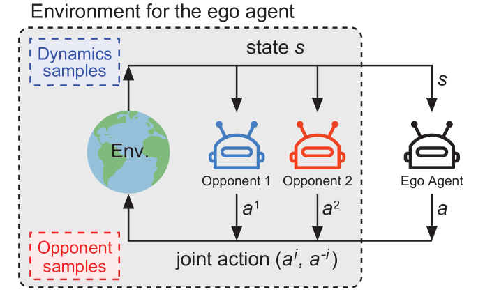
Figure 1: Two parts of the sample complexity in MARL.

As such, for an ego agent to achieve some policy performance in a multi-agent environment, the sample complexity is specified in two parts: (i) dynamics sample complexity, i.e., the number of state transition interactions between the agent group and the dynamics environment, and (ii) opponent sample complexity, i.e., the total number of opponent action sampling given the conditioned state. Figure 1 illustrates such two parts of sample complexity.

We argue that it is necessary to study such two parts of sample complexity explicitly since the two sub-processes’ approximations meet different challenges. Environment dynamics modeling is usually computationally expensive as the state representation and the joint actions are usually of high dimensions. Opponent modeling usually aims at approximating the opponents’ policies and eases MARL training in a decentralized manner Tian et al. (2020).

Opponent Sample Complexity as Communication.

If we leverage model-based techniques derived from SARL in multi-agent cases with decentralized setting, we may need to call real opponents for the action given the current state, which can be formulated as a communication protocol. For example, the agents communicate via calling for the opponent actions Tian et al. (2020): the ego agent sends a state (no matter real or simulated) to an opponent agent and receives the action sampled from the opponent’s policy. As such, we can regard the opponent sample complexity as communication load. To lower the opponent sample complexity, we replace the real opponents with learned opponent models in data simulation, which is analogous to selectively call some (or none) of opponents for useful information to reduce the communication load (or bandwidth) in multi-agent interactions Ryu et al. (2020).

4 Return Discrepancy Bounds

In this section, we conduct theoretical analysis to better understand model-based MARL in the decentralized setting, where each ego agent learns a dynamics model and opponent models based on observed data. For a comprehensive analysis, we also discuss the bound in centralized model-based MARL in Appendix A.

Usually, the dynamics model and opponent models have prediction errors, known as generalization errors. We investigate the influence of the learned models over the agent’s performance. From the perspective of agent $i$, we aim to bound the discrepancy between the expected return $\eta_{i}[\pi^{i},\pi^{-i}]$ of running the agent’s policy $\pi^{i}$ in the real dynamics $\mathcal{T}$ with real opponents $\pi^{-i}$ and the expected return $\hat{\eta}_{i}[\pi^{i},\hat{\pi}^{-i}]$ on a learned dynamics model $\hat{\mathcal{T}}(s^{\prime}|s,a^{i},a^{-i})$ with opponent models $\hat{\pi}^{-i}$. The return discrepancy upper bound $C$ can be expressed as

$$\left|\eta_{i}[\pi^{i},\pi^{-i}]-\hat{\eta}_{i}[\pi^{i},\hat{\pi}^{-i}]\right|\leq C~{}.$$ (1)

Once the upper bound $C$ is derived, it may indicate the key influence from the dynamics model and the opponent models, and thus helps design model-based algorithms accordingly.

In MARL with iterative policy optimization, we denote data-collecting policies in the previous iterations as $(\pi_{D}^{i},\pi_{D}^{-i})$. Then we measure the distribution shift between the current policies and the data-collecting policies with the total variation distance $\epsilon_{\pi}^{i}=\max_{s}D_{TV}(\pi^{i}(\cdot|s)\|\pi_{D}^{i}(\cdot|s))$, and similarly for the opponent agent $j\in\{-i\}$. Besides, interacting with $(\pi_{D}^{i},\pi_{D}^{-i})$, we denote the generalization error of the learned dynamics model $\hat{\mathcal{T}}$ compared to the real environment dynamics $\mathcal{T}$ as $\epsilon_{m}=\max_{t}\mathbb{E}_{(s_{t},a_{t}^{i},a_{t}^{-i})\sim\pi_{D}^{i},\pi_{D}^{-i}}$ $[D_{TV}(\mathcal{T}(\cdot|s_{t},a_{t}^{i},a_{t}^{-i})\|\hat{\mathcal{T}}(\cdot|s_{t},a_{t}^{i},a_{t}^{-i}))]$ and the error of the opponent model for agent $j$ as $\epsilon_{\hat{\pi}}^{j}=\max_{s}D_{TV}(\pi^{j}(\cdot|s)\|$ $\hat{\pi}^{j}(\cdot|s))$. Now we are ready to provide an upper bound.

Theorem 1.

Assume that the error of the learned dynamics model is bounded at each timestep by $\epsilon_{m}$, and the distance of the policies are bounded by $\epsilon_{\pi}^{i}$, $\epsilon_{\pi}^{j}$, and the errors of the opponent models are bounded by $\epsilon_{\hat{\pi}}^{j}$, for $j\in\{-i\}$. The return discrepancy upper bound can be expressed as

$$~{}\big{|}\eta_{i}[\pi^{i},\pi^{-i}]-\hat{\eta}_{i}[\pi^{i},\hat{\pi}^{-i}]\big{|}$$

$$\leq 2r_{\text{max}}\Big{[}\frac{\gamma(\epsilon_{m}+2\epsilon_{\pi}^{i}+2\sum_{j\in\{-i\}}\epsilon_{\pi}^{j}+\sum_{j\in\{-i\}}\epsilon_{\hat{\pi}}^{j})}{1-\gamma}$$ (2)

$$\quad\quad\quad\quad+2\epsilon^{i}_{\pi}+2\sum_{j\in\{-i\}}\epsilon_{\pi}^{j}+\sum_{j\in\{-i\}}\epsilon_{\hat{\pi}}^{j}\Big{]}.$$

Proof.

The proof is provided in Appendix B.2. ∎

This upper bound can be minimized by improving models’ accuracy, which is the standard objective in previous literature. We investigate the model usage instead, and a more instructive and practical upper bound is needed.

Here we first investigate a $k$-step rollout scheme, which is a natural extension of MBPO Janner et al. (2019) to multi-agent scenario. This rollout scheme begins from a state collected by the previous data-collecting policies, and then run the current policy for $k$ steps under the learned dynamics model and the opponent models. Denoting the return of using multi-agent branched rollouts as $\eta_{i}^{\text{branch}}$, and the bound of the generalization error of the learned dynamics model with the current policies $(\pi^{i},\pi^{-i})$ as $\epsilon_{m}^{\prime}=$ $\max_{t}\mathbb{E}_{(s_{t},a_{t}^{i},a_{t}^{-i})\sim\pi^{i},\pi^{-i}}[D_{TV}$ $(\mathcal{T}(\cdot|s_{t},a_{t}^{i},a_{t}^{-i})\|\hat{\mathcal{T}}(\cdot|s_{t},a_{t}^{i},a_{t}^{-i}))]~{},$ we derive the following return discrepancy upper bound.

Theorem 2.

Assume the generalization error is bounded by $\epsilon_{m}^{\prime}$ and the distance of the policies are bounded as $\epsilon_{\pi}^{i}$, $\epsilon_{\pi}^{j}$ and $\epsilon_{\hat{\pi}}^{j}$ for $j\in\{-i\}$. The bound of the discrepancy between the return in real environment $\eta_{i}[\pi^{i},\pi^{-i}]$ and the return using the dynamics model and opponent models with branched rollouts $\eta_{i}^{\text{branch}}[(\pi^{1}_{D},\hat{\pi}^{1}),\ldots,(\pi^{i}_{D},\pi^{i}),\ldots,(\pi^{n}_{D},\hat{\pi}^{n})]$ is

$$\big{|}\eta_{i} [\pi^{i},\pi^{-i}]-\eta_{i}^{\text{branch}}[(\pi^{1}_{D},\hat{\pi}^{1}),\ldots,(\pi^{i}_{D},\pi^{i}),\ldots,(\pi^{n}_{D},\hat{\pi}^{n})]\big{|}$$

$$\leq 2r_{\text{max}}\Big{[}\underbrace{k\epsilon_{m}^{\prime}+(k+1)\sum_{j\in\{-i\}}\epsilon_{\hat{\pi}}^{j}}_{\text{model generalization error}}$$

$$\quad+\underbrace{\gamma^{k+1}\big{(}\epsilon_{\pi}^{i}+\sum_{j\in\{-i\}}\epsilon_{\pi}^{j}\big{)}+\frac{\gamma^{k+1}(\epsilon_{\pi}^{i}+\sum_{j\in\{-i\}}\epsilon_{\pi}^{j})}{1-\gamma}}_{\text{policy distribution shift}}\Big{]}$$

$$=C(\epsilon_{m}^{\prime},\epsilon_{\pi}^{i},\epsilon_{\pi}^{-i},\epsilon_{\hat{\pi}}^{-i},k)~{},$$ (3)

where $\epsilon_{\pi}^{-i}=\sum_{j\in\{-i\}}\epsilon_{\pi}^{j}$, $\epsilon_{\hat{\pi}}^{-i}=\sum_{j\in\{-i\}}\epsilon_{\hat{\pi}}^{j}$ and the pair $(\pi_{D}^{j},\hat{\pi}^{j})$ means that the policy $\pi_{D}^{j}$ and opponent model $\hat{\pi}^{j}$ are used before and after the branch point respectively for agent $j$.

Proof.

The proof is provided in Appendix B.2. ∎

The upper bound $C(\epsilon_{m}^{\prime},\epsilon_{\pi}^{i},\epsilon_{\pi}^{-i},\epsilon_{\hat{\pi}}^{-i},k)$ in Eq. (3) consists of the generalization errors of both dynamics model and opponent models as well as the policy distribution shift. Intuitively, choosing the optimal $k^{*}=\arg\min_{k>0}C(\epsilon_{m}^{\prime},\epsilon_{\pi}^{i},\epsilon_{\pi}^{-i},\epsilon_{\hat{\pi}}^{-i},k)$ with sufficiently low $\epsilon_{m}^{\prime}$ and $\sum_{j\in\{-i\}}\epsilon_{\hat{\pi}}^{j}$ minimizes the discrepancy, which, however, cannot directly achieve a low discrepancy if any opponent model has relatively large error. So we need to reduce the upper bound such that the policy trained with the model rollouts will still perform well in real environment, leading to improved sample efficiency. To be more specific, we can optimize the target $\eta_{i}$ through optimizing $\eta_{i}^{\text{branch}}$ if the bound is tight. And improving $\eta_{i}^{\text{branch}}$ by $C(\epsilon_{m}^{\prime},\epsilon_{\pi}^{i},\epsilon_{\pi}^{-i},\epsilon_{\hat{\pi}}^{-i},k)$ guarantees to improve the target $\eta_{i}$. It means that the policy improved under the environment model and the opponent models will get improved performance in the real environment.

Remark.

As the policy is trained using mainly the samples from the model rollouts, which do not contribute to the sample complexity. A reduced return discrepancy upper bound indicates that the policy will get more improvement in the real environment given that the policy is improved to the same degree using the models. In other words, the policy will obtain the same performance improvement in the real environment with fewer samples with a reduced discrepancy upper bound.

Now the problem becomes how to reduce the bound in order to achieve low sample complexity. Considering that $\epsilon_{\hat{\pi}}^{j}$ may be different across different opponent models, and sometimes the ego agent can call the real opponent agents for real actions, the rollout length $k$ needs not to be the same across different opponents. Thus, in Section 5 we propose a method called Adaptive Opponent-wise Rollout Policy Optimization (AORPO) to reduce the upper bound.

5 The AORPO Method

Based on the bound analysis in Theorem 2, now we present the detailed AORPO algorithm and prove its convergence.

1 Initialize policy $\pi_{\zeta}$, Q value function $Q_{\omega}$, predictive model $\hat{\mathcal{T}}_{\theta}$, opponent models $\pi_{\phi^{j}}$ for $j\in\{-i\}$, environment dataset $\mathcal{D}_{\text{env}}$, model dataset $\mathcal{D}_{\text{model}}$.

2 for $N$ epochs do

3       Train model $\hat{\mathcal{T}}_{\theta}$ on $\mathcal{D}_{\text{env}}$.

4       for $E$ steps do

5             Take actions in environment via $\pi_{\zeta}$ with real opponents, add the transitions to $\mathcal{D}_{\text{env}}$.

6             Train all opponent models $\pi_{\phi^{j}}$.

7             Compute the errors for each opponent model $\epsilon_{\hat{\pi}}^{j}$.

8             For each opponent, compute $n^{j}=\lfloor k\frac{\min_{j^{\prime}}\epsilon_{\hat{\pi}}^{j^{\prime}}}{\epsilon_{\hat{\pi}}^{j}}\rfloor$.

9             for $M$ model rollouts do

10                   Sample $s_{t}$ uniformly from $\mathcal{D}_{\text{env}}$.

11                   Perform $k$-step rollouts from $s_{t}$:

12                   for $p=1,\ldots,k$ do

13                         $a_{t+p-1}^{i}=\pi_{\zeta}(s_{t+p-1})$

14                         For each opponent $j$:

15                         if $p\leq n^{j}$ then

16                               $a_{t+p-1}^{j}=\pi_{\phi^{j}}(s_{t+p-1})$

17                        else

18                               $a_{t+p-1}^{j}$ = Comm ($s_{t+p-1}$, $j$)

19                        $s_{t+p}=\hat{\mathcal{T}}_{\theta}(s_{t+p-1},a_{t+p-1}^{i},a_{t+p-1}^{-i})$

20                   Add the transitions to $\mathcal{D}_{\text{model}}$.

21            Train the Q function and the policy using data from $\mathcal{D}_{\text{model}}$ with the loss in Eq. (5) and Eq. (4).

22      

23 Function Comm ($s$, $j$) :

24       Send state $s$ to agent $j$.

25       return the received $a^{j}$

Algorithm 1 AORPO Algorithm

5.1 Algorithm Details of AORPO

We propose a model-based MARL algorithm named Multi-Agent Branched-Rollout Policy Optimization (AORPO). The overall algorithm of AORPO is shown in Algorithm 1. For simplicity, the detailed algorithm is described in the perspective of agent $i$. AORPO includes some key components, and the implementation of them is based on previous work, which serve as the preliminaries and are described in Appendix E.

In AORPO, the agent $i$ learns a dynamics model and an opponent model for each of other agents and learns a policy based on the data collected from the model rollouts.

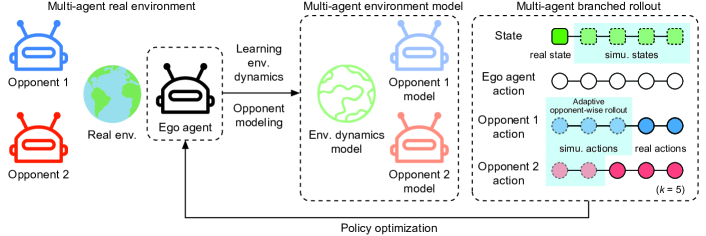
Figure 2: Illustration of the adaptive opponent-wise rollout policy optimization (AORPO) method from the perspective of the ego agent. The ego agent begins the rollouts from the states collected from the real environment interacting with real opponents, then runs $k$ steps under the learned dynamics model. For each opponent agent, the ego agent interacts with it directly or with the opponent model for it in the $k$-step rollout, according to the prediction performance of its opponent model.

5.1.1 Agent Learning

For the dynamics model, in line 1 of Algorithm 1, a bootstrap ensemble of probabilistic dynamics models is trained to predict the environment dynamics as in Chua et al. Chua et al. (2018), and we select one of the models randomly from a uniform distribution when generating a prediction. For the opponent model, in line 1 of Algorithm 1, the policy of one opponent agent $j$ can be modeled as a Gaussian distribution of the action. We further use the opponent models to encourage the coordination behaviors. Agent $i$ makes a decision based on both the current state and the inferred opponent actions $\hat{a}^{-i}$.

For the policy learning, AORPO is implemented based on the Multi-Agent Soft Actor-Critic (MASAC) algorithm, which is a multi-agent version of Soft Actor-Critic algorithm Haarnoja et al. (2018). In line 1 of Algorithm 1, agent $i$ alternates between optimizing its policy and updating the value function. With the reparameterization function $f$ and a Gaussian $\mathcal{N}$, the policy optimization objective is

$$J(\pi)=\mathbb{E}_{s_{t},a_{t}^{-i}\sim\mathcal{D},\epsilon_{t}\sim\mathcal{N}}[ \alpha\log\pi(f(\epsilon_{t};s_{t})|s_{t},\hat{a}_{t}^{-i})$$ (4)

$$-Q(s_{t},f(\epsilon_{t};s_{t}),a^{-i}_{t})]~{},$$

where $\mathcal{D}$ is the replay buffer, $\epsilon_{t}$ is the input noise and $\hat{a}_{t}^{-i}\sim\hat{\pi}^{-i}(\cdot|s_{t})$.

The loss function of the Q function is

$$J(Q)=\mathbb{E}_{s_{t},a_{t}^{i},a_{t}^{-i}\sim\mathcal{D}}\Big{[}\frac{1}{2}\Big{(}Q(s_{t},a_{t}^{i},a_{t}^{-i})$$ (5)

$$-\big{(}r_{t}+\gamma Q(s_{t+1},a_{t+1}^{i},a_{t+1}^{-i})-\alpha\log\pi(a_{t+1}^{i}|s_{t+1})\big{)}\Big{)}^{2}\Big{]}~{},$$

where $\alpha$ is the temperature hyperparameter.

5.1.2 Adaptive Opponent-wise Rollout

In this work, a $k$-step model rollout begins from a real state collected in the real environment. We design the adaptive opponent-wise rollout scheme to reduce the bound. The opponent model generalization error term $(k+1)\sum_{j\in\{-i\}}\epsilon_{\hat{\pi}}^{j}$ of the bound in Eq. (3) reveals that different magnitudes of opponent model errors may lead to different contributions to the compounding error of the multi-step simulated rollouts. Intuitively, if too short rollouts are performed, the relatively accurate opponent models are not fully utilized, leading to low sample efficiency. In contrast, if the rollout is too long, the relatively inaccurate opponent models may cause the rollouts to depart from the real trajectory distribution heavily, leading to degraded performance in the environment and thereby low sample efficiency. Thus our proposed adaptive opponent-wise rollout scheme lowers the rollout length of the relatively inaccurate opponent models but keeps long rollout length for relatively accurate opponent models, as shown in Figure 2.

We can achieve this since the agent $i$ can play with either the learned opponent model $\hat{\pi}^{j}$ or the real policy $\pi^{j}$ of each opponent $j$. In detail, for the opponent $j$, $\hat{\pi}^{j}$ is used for the first $n^{j}=\lfloor k\frac{\min_{j^{\prime}}\epsilon_{\hat{\pi}}^{j^{\prime}}}{\epsilon_{\hat{\pi}}^{j}}\rfloor$ steps, then the agent $i$ interacts with the real opponent $\pi^{j}$ in the rest $k-n^{j}$ steps. The compounding error contribution of each opponent model is thus bounded by $k\min_{j^{\prime}}{\epsilon_{\hat{\pi}}^{j^{\prime}}}$. Note that the adaptive opponent-wise rollout scheme requires the ego agent $i$ can obtain the actions $a_{t}^{j}$ from the real policy in the last $k-n^{j}$ steps. In algorithm 1 of Algorithm 1, the ego agent $i$ sends the simulated states to the opponent $j$ and requires the response, following the predefined communication protocol. One may argue that it will introduce extra opponent sample complexity since we need to communicate with the real opponent in the model rollouts. However, if we only use the opponent models, more errors are exploited, and it will lead to a poor policy and, finally, the sample complexity to achieve some good performance will be high. Our experiments in Section 6 will justify this claim.

With such $n^{j}$’s, the generalization error caused by the opponent models becomes $\sum_{j\in\{-i\}}(n^{j}+1)\epsilon_{\hat{\pi}}^{j}\simeq(n-1)k\min_{j^{\prime}}\epsilon_{\hat{\pi}}^{j^{\prime}}$, which is remarkably reduced and makes a good balance of the contribution to overall generalization error from different opponent models. According to the remark of Theorem 2, improving the surrogate return $\eta_{i}^{\text{branch}}$ with a tighter discrepancy bound will improve the target return $\eta_{i}$ more efficiently. Note that the comparison of different model usage schemes is provided in Appendix G.6, where the above scheme yields the highest asymptotic performance and sample efficiency.

5.2 Convergence Guarantee

According to Wei et al. Wei et al. (2018), the optimal policy learned by MASQL is $\pi^{*}_{\text{MASQL}}=\exp{(\frac{1}{\alpha}Q^{*}(s_{t},\cdot)-V^{*}(s_{t}))}=\exp{(\frac{1}{\alpha}Q^{*}(s_{t},\cdot))}/\exp{\left(V^{*}(s_{t})\right)}$, where $Q^{*}$ and $V^{*}$ are the optimal Q function and state value function respectively. As Haarnoja et al. Haarnoja et al. (2018) showed, the optimal policy learned by MASAC should be $\pi^{*}_{\text{MASAC}}=\exp{(\frac{1}{\alpha}Q^{*}(s_{t},\cdot))}/Z(s_{t})$. Since the partition function is $Z(s_{t})=\exp{\left(V^{*}(s_{t})\right)}$, with given the same optimal $Q^{*}$ and $V^{*}$, MASQL is equivalent to MASAC from the perspective of policy learning. With this fact, we prove that (1) using the learned dynamics model and the opponent models in AORPO still guarantees the convergence of MASQL; (2) MASQL still guarantees the convergence of Nash Q-learning Hu and Wellman (2003). Thus we prove that AORPO achieves the convergence solution of Nash Q-learning. The theorems and proofs can be found in Appendix D, Theorem 6 and Theorem 7.

The theorems guarantee AORPO’s convergence under several assumptions. However, we show that the assumptions are not necessary conditions for the learning algorithm to converges by the following experimental results in Figure 4, in which the convergence is still guaranteed when the assumptions are not strictly satisfied. More empirical findings can be found in Yang et al. Yang et al. (2018).

6 Experiments

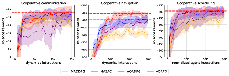
Figure 3: The average episode reward performance of five different random seeds in the cooperative tasks. Dynamics interactions means the episodes in the training stage (the agents interacts with the dynamics environment 25 times in an episode). Normalized agent interactions means the times the agent groups complete a full interaction, which is divided by 25.

We evaluate the performance of AORPO in both competitive and cooperative tasks. We demonstrate that AORPO can converge to the Nash equilibrium and that AORPO is more sample-efficient than a series of baselines in both competitive and cooperative tasks. See Appendix G for task details.

Compared Methods.

We compare our method AORPO with the strong model-free MARL algorithms, MADDPG Lowe et al. (2017) and MASAC. To show that our multi-agent models approach is generally helpful and to have fair comparisons, we also implement AORPO on top of MADDPG, named as AORDPG, for more comprehensive analysis.

Implementation.

As for the practical implementation of AORPO, we first collect real experience data using model-free algorithms and use them to pre-train the dynamics model and the opponent models. Other implementation details, including network architectures and important hyperparameters, are provided in Appendix F.

6.1 Competitive Tasks

Climb is a modified Battle of Sex game. Agent 1 picks a number $a\in[-1,1]$, and agent 2 picks a number $b\in[-1,1]$. Their actions form a position $(a,b)$. There are 2 states and 2 corresponding landmarks located in the lower-left $(-0.5,-0.5)$ and in the upper right $(0.5,0.5)$ respectively. The only Nash equilibrium is that the agents go to the lower-left landmark at state 1 and go to the upper right landmark at state 2.

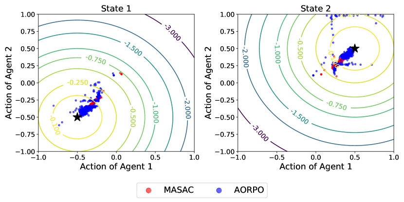
Figure 4: Climb task convergence.

The reward surfaces of converged MASAC and AORPO for the two agents in the two states are shown in Figure 4. The result verifies that AORPO will converge to the Nash equilibrium. In Appendix G.3 and G.4, we further provide more detailed results of comparing model-based and model-free methods conducted in several competitive environments of the Multi-Agent Particle Environment Lowe et al. (2017) and the results of comparing AORPO with another model-based MARL, i.e., MAMSGM Krupnik et al. (2019).

6.2 Cooperative Tasks

Based on a multi-agent particle environment, we evaluate our method in two types of cooperative tasks: CESO tasks for complex environment dynamics and simple opponents, while SECO tasks for simple environment dynamics and complex opponents. CESO tasks include Cooperative communication with two agents and three landmarks and Cooperative navigation with three agents and three landmarks. The studied SECO task is Cooperative scheduling with three agents and three landmarks, as detailed in Appendix G.

The laws of mechanics and the collisions’ stochastic outcomes make difficulties for the dynamics model prediction, so we mainly consider the efficiency of interacting with the environment in the CESO tasks. In the left and middle subfigures of Figure 3, both AORPO and AORDPG can reach the asymptotic performance of the state-of-the-art model-free baselines with fewer interactions with the environment, i.e., achieving lower dynamics sample complexity.

The Cooperative scheduling task is configured as a SECO task, with two kinds of agents and two kinds of action spaces. We consider the efficiency of interacting with the other agents in the SECO tasks. As shown in the right subfigure of Figure 3, our methods AORPO and AORDPG reach the asymptotic performance with fewer agents’ interactions, which means the opponent sample complexity is lower. One may think using opponent models will indeed introduce extra agent interactions when running rollouts, but interestingly, AORPO uses fewer agent interactions to achieve some performance since it helps policy learn faster. More detailed experiments are presented in Appendix G.

6.3 Analysis on Model Usage

We further discuss the effect of the opponent model usage. Although the generalization errors caused by the opponent models in the return discrepancy are hard to estimate, the opponent models affect the performance through the model compounding errors. We investigate the model compounding errors when using adaptive opponent-wise rollout or using the opponent models in a whole rollout. Specifically, for a real trajectory $(s_{0},a_{0},\ldots,s_{h})$, a branched rollout from the start state $s_{0}$ under learned dynamics model and opponent models is denoted as $(s_{0},\hat{a}_{0},\ldots,\hat{s}_{h})$. Following Nagabandi et al. Nagabandi et al. (2018), the model compounding error is defined as $\epsilon_{\text{c}}=\frac{1}{h}\sum_{i=1}^{h}\|s_{i}-\hat{s}_{i}\|^{2}_{2}$.

Using opponent models reduces interactions among agents but causes extra compounding errors compared with real opponents. We show the trade-off between model errors and interaction times in Figure 5, where the left and right y-axes are for the solid lines and the dotted lines, respectively. We observe the adaptive opponent-wise rollout achieves lower model compounding error than rollout with all opponent models while reducing the number of interactions compared to rollout with real opponents.

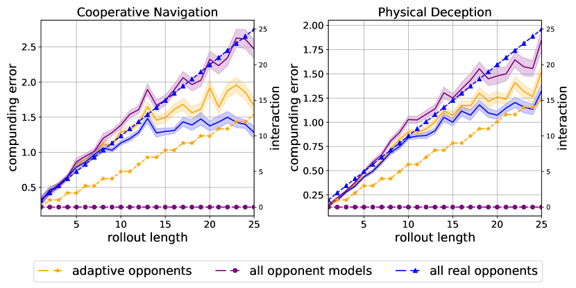
Figure 5: Model compounding errors and interactions numbers of different model usages.

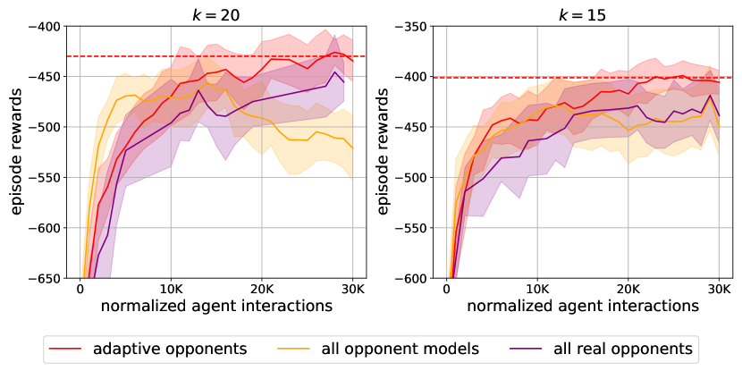
Figure 6: Performance curves of average episode reward of different model usages.

Moreover, we investigate how different rollout schemes affect the sample efficiency. In Figure 6, we compare three kinds of usages in a Cooperative navigation scenario using two settings of rollout length $k$. We notice that using the adaptive opponent-wise rollout achieves the same performance with fewer interactions among the agents than interacting with all real opponents, verifying that although we introduce some sample complexity while simulating data, the reduced discrepancy bound ensures the model-based methods to improve the sample efficiency. It can also avoid performance drop caused by compounding error compared with using all opponent models, which means that the adaptive opponent-wise rollout scheme mitigates some bad opponent models’ negative effect by leveraging different rollout lengths of opponent models.

7 Conclusion

In this paper, we investigated model-based MARL problems with both theoretical and empirical analyses. We specified two parts of sample complexity in MARL and derived an upper bound of the return discrepancy in model-based MARL w.r.t. the policy distribution shift and the generalization errors of the learned dynamics model and opponent models. Inspired by the theoretical analysis, we designed the AORPO algorithm framework, in which the return discrepancy can be reduced by adaptive opponent-wise rollout controlling and the two parts of sample complexity are strategically reduced by the learned dynamics and opponent models. We then proved that AORPO can converge to Nash Q-values with reasonable assumptions. In experiments, AORPO has shown highly comparable asymptotic performance with the model-free MARL baselines while achieving higher sample efficiency. For future work, we plan to look deeper into various adaptive opponent-wise rollout schemes for different settings of model-based MARL. We will also investigate theoretical and empirical results of multi-agent dynamics model learning to further ease model-based MARL and improve its sample efficiency.

Appendix

Appendix A Upper Bounds for Centralized Model-based MARL

In this section, we derive an upper bound of the return discrepancy between the expected return under the real environment and the expected return under a learned dynamics model, both from the perspective of the ego agent, i.e., agent $i$, interacting with the known real opponent agents, which corresponds to centralized MARL settings and will not produce extra opponent sample complexity.

Theorem 3.

Assume that the expected total variation distance between the learned dynamics model $\hat{\mathcal{T}}$ and the real dynamics model $\mathcal{T}$ is bounded at each timestep under the expectation of $\pi_{D}^{i}$ and $\pi_{D}^{-i}$ by $\epsilon_{m}=\max_{t}\mathbb{E}_{(s_{t},a_{t}^{i},a_{t}^{-i})\sim\pi_{D}^{i},\pi_{D}^{-i}}[D_{TV}$ $(\mathcal{T}(\cdot|s_{t},a_{t}^{i},a_{t}^{-i})\|\hat{\mathcal{T}}(\cdot|s_{t},a_{t}^{i},a_{t}^{-i}))]$, and the distance of the policies are bounded as $\epsilon_{\pi}^{i}=\max_{s}D_{TV}(\pi^{i}(\cdot|s)\|\pi_{D}^{i}(\cdot|s))$, $\epsilon_{\pi}^{-i}=\max_{s}D_{TV}($ $\pi^{-i}(\cdot|s)\|\pi_{D}^{-i}(\cdot|s))$, where subscript $D$ means the certain policies are used to collect data. Then the returns under the real dynamics and the learned dynamics model are bounded as:

$$\left|\eta_{i}[\pi^{i},\pi^{-i}]-\hat{\eta}_{i}[\pi^{i},\pi^{-i}]\right|\leq 2r_{\text{max}}\Big{[}\frac{\gamma(\epsilon_{m}+2\epsilon_{\pi}^{i}+2\epsilon_{\pi}^{-i})}{1-\gamma}+2\epsilon^{i}_{\pi}+2\epsilon^{-i}_{\pi}\Big{]}~{},$$

where $\hat{\eta}$ means that the policies are executed under the learned dynamics model.

Proof.

We can use Lemma C.3 to bound the returns, and it requires to bound the error of the learned dynamics model. Thus we need to introduce $\pi^{i}_{D}$ and $\pi^{-i}_{D}$ by adding and subtracting $\eta[\pi^{i}_{D},\pi^{-i}_{D}]$:

$$\left|\eta_{i}[\pi^{i},\pi^{-i}]-\hat{\eta}_{i}[\pi^{i},\pi^{-i}]\right|\leq\underbrace{\left|\eta_{i}[\pi^{i},\pi^{-i}]-\eta_{i}[\pi^{i}_{D},\pi^{-i}_{D}]\right|}_{L_{1}}+\underbrace{\left|\eta_{i}[\pi^{i}_{D},\pi^{-i}_{D}]-\hat{\eta}_{i}[\pi^{i},\pi^{-i}]\right|}_{L_{2}}~{}.$$

We can bound both $L_{1}$ and $L_{2}$ using Lemma C.3.

For $L_{1}$, we apply Lemma C.3 using $M=0$, $\mathcal{P}=\epsilon_{\pi}^{i}$, $O=\epsilon_{\pi}^{-i}$, and obtain

$$L_{1}\leq 2r_{\text{max}}\Big{[}\frac{\gamma(\epsilon_{\pi}^{i}+\epsilon_{\pi}^{-i})}{1-\gamma}+\epsilon^{i}_{\pi}+\epsilon^{-i}_{\pi}\Big{]}~{}.$$

For $L_{2}$, we apply Lemma C.3 using $M=\epsilon_{m}$, $P=\epsilon_{\pi}^{i}$, $O=\epsilon_{\pi}^{-i}$, and obtain

$$L_{2}\leq 2r_{\text{max}}\Big{[}\frac{\gamma(\epsilon_{m}+\epsilon_{\pi}^{i}+\epsilon_{\pi}^{-i})}{1-\gamma}+\epsilon^{i}_{\pi}+\epsilon^{-i}_{\pi}\Big{]}~{}.$$

Adding the two bounds together completes the proof. ∎

Extended Theorem A.1.

Assume that the expected total variation distance between the learned dynamics model and the real dynamics model is bounded at each timestep under the expectation of $\pi_{D}^{i}$ and $\pi_{D}^{-i}$ by $\epsilon_{m}=\max_{t}\mathbb{E}_{(s_{t},a_{t}^{i},a_{t}^{-i})\sim\pi_{D}^{i},\pi_{D}^{-i}}[D_{TV}(\mathcal{T}(\cdot|s_{t},a_{t}^{i},a_{t}^{-i})\|\hat{\mathcal{T}}(\cdot|s_{t},a_{t}^{i},a_{t}^{-i}))]$ , and the distance of the policies are bounded as $\epsilon_{\pi}^{i}=\max_{s}D_{TV}(\pi^{i}(\cdot|s)\|\pi_{D}^{i}(\cdot|s))$, $\epsilon_{\pi}^{j}=\max_{s}D_{TV}(\pi^{j}(\cdot|s)\|\pi_{D}^{j}(\cdot|s))$ for $j\in\{-i\}$. Then the returns under the real dynamics and the learned dynamics model are bounded as:

$$\left|\eta_{i}[\pi^{i},\pi^{-i}]-\hat{\eta}_{i}[\pi^{i},\pi^{-i}]\right| \leq 2r_{\text{max}}\Big{[}\frac{\gamma(\epsilon_{m}+2\epsilon_{\pi}^{i}+2\sum_{j\in\{-i\}}\epsilon_{\pi}^{j})}{1-\gamma}+2\epsilon^{i}_{\pi}+2\sum_{j\in\{-i\}}\epsilon_{\pi}^{j}\Big{]}$$

$$=C(\epsilon_{m},\epsilon_{\pi}^{i},\epsilon_{\pi}^{-i})~{},$$

where $\epsilon_{\pi}^{-i}=\sum_{j\in\{-i\}}\epsilon_{\pi}^{j}$ is the distribution shift caused by the opponent agent policies.

Proof.

Following the similar procedures of proving Theorem 3 while using Extended Lemmas (C.1-C.4) completes the proof. ∎

The discrepancy bound of the returns in A.1 is denoted as $C(\epsilon_{m},\epsilon_{\pi}^{i},\epsilon_{\pi}^{-i})$, in which the generalizatoin error of the dynamics model $\epsilon_{m}$ is the only controllable variable, i.e., can be reduced by improving the performance of the dynamics model. However, in a centralized model-based MARL method, amounts of interactions between the agents are required, which leads to low sample efficiency.

Appendix B Upper Bounds for Model-based Multi-agent Policy Optimization with Adaptive Opponent-wise Rollouts

In this section, we prove the upper bounds presented in the main paper for decentralized model-based MARL, from the perspective of the ego agent, i.e., agent $i$, where opponent modeling is required to infer the actions of opponent agents. Specifically, We first prove the upper bounds for the situations where the ego agent plays with one opponent, and then prove the upper bounds for the situations where the ego agent plays with multiple opponents.

B.1 Single Opponent Case

Theorem 4.

Assume that the expected total variation distance between the learned dynamics model $\hat{\mathcal{T}}$ and the real dynamics model $\mathcal{T}$ is bounded at each timestep under the expectation of $\pi_{D}^{i}$ and $\pi_{D}^{-i}$ by $\epsilon_{m}=\max_{t}\mathbb{E}_{(s_{t},a_{t}^{i},a_{t}^{-i})\sim\pi_{D}^{i},\pi_{D}^{-i}}[D_{TV}(\mathcal{T}(\cdot|s_{t},a_{t}^{i},a_{t}^{-i})\|$ $\hat{\mathcal{T}}(\cdot|s_{t},a_{t}^{i},a_{t}^{-i}))]$, the distribution shift of the policies are bounded as $\epsilon_{\pi}^{i}=\max_{s}D_{TV}(\pi^{i}(\cdot|s)\|\pi_{D}^{i}(\cdot|s))$, $\epsilon_{\pi}^{-i}=\max_{s}D_{TV}(\pi^{-i}(\cdot|s)\|\pi_{D}^{-i}(\cdot|s))$, the generalization error of the opponent model is bounded as $\epsilon_{\hat{\pi}}=\max_{s}D_{TV}(\pi^{-i}(\cdot|s)\|$ $\hat{\pi}^{-i}(\cdot|s))$. Then the discrepancy of returns under the real dynamics and the learned dynamics with opponent models is bounded as

$$\left|\eta_{i}[\pi^{i},\pi^{-i}]-\hat{\eta}_{i}[\pi^{i},\hat{\pi}^{-i}]\right|\leq 2r_{\text{max}}\Big{[}\frac{\gamma(\epsilon_{m}+2\epsilon_{\pi}^{i}+2\epsilon_{\pi}^{-i}+\epsilon_{\hat{\pi}}^{-i})}{1-\gamma}+2\epsilon^{i}_{\pi}+2\epsilon_{\pi}^{-i}+\epsilon_{\hat{\pi}}^{-i}\Big{]}.$$

Proof.

By adding and subtracting a same term $\hat{\eta}_{i}[\pi^{i},\pi^{-i}]$, we have

$$\left|\eta_{i}[\pi^{i},\pi^{-i}]-\hat{\eta}_{i}[\pi^{i},\hat{\pi}^{-i}]\right|\leq\underbrace{|\eta_{i}[\pi^{i},\pi^{-i}]-\hat{\eta}_{i}[\pi^{i},\pi^{-i}]|}_{L_{1}}+\underbrace{|\hat{\eta}_{i}[\pi^{i},\pi^{-i}]-\hat{\eta}_{i}[\pi^{i},\hat{\pi}^{-i}]|}_{L_{2}}~{}.$$

We can bound both $L_{1}$ and $L_{2}$ using Theorem 3 and Lemma C.3.

For $L_{1}$, we apply Theorem 3 and obtain

$$L_{1}\leq 2r_{\text{max}}\Big{[}\frac{\gamma(\epsilon_{m}+2\epsilon_{\pi}^{i}+2\epsilon_{\pi}^{-i})}{1-\gamma}+2\epsilon^{i}_{\pi}+2\epsilon^{-i}_{\pi}\Big{]}~{}.$$

For $L_{2}$, we apply Lemma C.3 using $M=0$, $P=0$, $O=\epsilon_{\hat{\pi}}^{-i}$, and obtain

$$L_{2}\leq 2r_{\text{max}}\Big{[}\frac{\gamma\epsilon_{\hat{\pi}}^{-i}}{1-\gamma}+\epsilon_{\hat{\pi}}^{-i}\Big{]}~{}.$$

Adding together the two bounds completes the proof. ∎

Theorem 5.

Assume that the expected total variation distance between the learned dynamics model and the real dynamics transition is bounded at each timestep under the expectation of $\pi^{i}$ and $\pi^{-i}$ by $\epsilon_{m}^{\prime}=\max_{t}\mathbb{E}_{(s_{t},a_{t}^{i},a_{t}^{-i})\sim\pi^{i},\pi^{-i}}[D_{TV}(\mathcal{T}(\cdot|s_{t},a_{t}^{i},a_{t}^{-i})\|$ $\hat{\mathcal{T}}(\cdot|s_{t},a_{t}^{i},a_{t}^{-i}))]$, the distribution shift of the policies are bounded as $\epsilon_{\pi}^{i}=\max_{s}D_{TV}(\pi^{i}(\cdot|s)\|\pi_{D}^{i}(\cdot|s))$, $\epsilon_{\pi}^{-i}=\max_{s}D_{TV}$ $(\pi^{-i}(\cdot|s)\|\pi_{D}^{-i}(\cdot|s))$, and the generalization error of the opponent model is bounded as $\epsilon_{\hat{\pi}}^{-i}=\max_{s}D_{TV}(\pi^{-i}(\cdot|s)\|\pi_{\phi}^{-i}(\cdot|s))$. Then the upper bound of the return discrepancy is

$$\Big{|}\eta_{i}[\pi^{i},\pi^{-i}]-\eta_{i}^{\text{branch}}[(\pi^{i}_{D},\pi^{i}),(\pi^{-i}_{D},\hat{\pi}^{-i})]\Big{|}$$

$$\leq 2r_{\text{max}}\Big{[}k\epsilon_{m}^{\prime}+\gamma^{k+1}(\epsilon_{\pi}^{i}+\epsilon_{\pi}^{-i})+\frac{\gamma^{k+1}(\epsilon_{\pi}^{i}+\epsilon_{\pi}^{-i})}{1-\gamma}+(k+1)\epsilon_{\hat{\pi}}^{-i}\Big{]}~{}.$$

Proof.

In order to introduce the model generalization error, we select the reference term as the return of a branched rollout $\eta_{i}^{\text{branch}}[(\pi_{D}^{i},\pi^{i}),$ $(\pi_{D}^{-i},\pi^{-i})]$, which executes $\pi_{D}^{i}$ and $\pi_{D}^{-i}$ in the real environment until the branch point and executes $\pi^{i}$ and $\pi^{-i}$ for $k$ steps with the dynamics model after the branch point. As such, we have

$$\big{|}\eta_{i}[\pi^{i},\pi^{-i}]-\eta_{i}^{\text{branch}}[(\pi^{i}_{D},\pi^{i}),(\pi^{-i}_{D},\hat{\pi}^{-i})]\big{|}$$

$$\leq~{}\underbrace{\big{|}\eta_{i}[\pi^{i},\pi^{-i}]-\eta_{i}^{\text{branch}}[(\pi_{D}^{i},\pi^{i}),(\pi_{D}^{-i},\pi^{-i})]\big{|}}_{L_{1}}+\underbrace{\big{|}\eta_{i}^{\text{branch}}[(\pi_{D}^{i},\pi^{i}),(\pi_{D}^{-i},\pi^{-i})]-\eta_{i}^{\text{branch}}[(\pi^{i}_{D},\pi^{i}),(\pi^{-i}_{D},\hat{\pi}^{-i})]\big{|}}_{L_{2}}~{},$$

where we can bound both $L_{1}$ and $L_{2}$ using Lemma C.4.

$L_{1}$ suffers from the policy errors before the branch point and the model generalization error after the branch point. By applying Lemma C.4 with the bounds $P^{\text{pre}}=\epsilon^{i}_{\pi}$, $O^{\text{pre}}=\epsilon_{\pi}^{-i}$, $M^{\text{post}}=\epsilon_{m}^{\prime}$ and setting other errors to $0$, we have

$$L_{1}\leq 2r_{\text{max}}\Big{[}k\epsilon_{m}^{\prime}+\gamma^{k+1}(\epsilon_{\pi}^{i}+\epsilon_{\pi}^{-i})+\frac{\gamma^{k+1}(\epsilon^{i}_{\pi}+\epsilon^{-i}_{\pi})}{1-\gamma}\Big{]}~{}.$$

$L_{2}$ only suffers from the opponent model errors after the branch point, and we can apply Lemma C.4 with the bounds $O^{\text{post}}=\epsilon_{\hat{\pi}}^{-i}$ and set other errors to $0$, which leads to

$$L_{2}\leq 2r_{\text{max}}[(k+1)\epsilon_{\hat{\pi}}^{-i}]~{}.$$

Adding the two bounds completes the proof. ∎

B.2 Multiple Opponents Case

Now we extend the theorems above to the situations where there are $n$ agents. From the perspective of the ego agent, i.e., agent $i$, we assume that the opponent agents $\{-i\}$ are making decisions independently and agent $i$ takes actions depending on the opponent models of other agents $\{-i\}$, which factorizes the joint distribution as

$$p(s,a^{1},\ldots,a^{i},\ldots,a^{n})=p(s)\pi^{i}(a^{i}|s,a^{1},\ldots,a^{i-1},a^{i+1},\ldots,a^{n})\prod_{j\in\{-i\}}\pi^{j}(a^{j}|s)~{}.$$

Extended Theorem B.1.

Assume that the expected total variation distance between the learned dynamics model and the real dynamics model is bounded at each timestep under the expectation of $\pi_{D}^{i}$ and $\pi_{D}^{-i}$ by $\epsilon_{m}=\max_{t}\mathbb{E}_{(s_{t},a_{t}^{i},a_{t}^{-i})\sim(\pi_{D}^{i},\pi_{D}^{-i})}[D_{TV}($ $\mathcal{T}(\cdot|s,a^{i},a^{-i})\|\hat{\mathcal{T}}(\cdot|s,a^{i},a^{-i}))]$, the distribution shift of the policies are bounded as $\epsilon_{\pi}^{i}=\max_{s}D_{TV}(\pi^{i}(\cdot|s)\|\pi_{D}^{i}(\cdot|s))$, $\epsilon_{\pi}^{j}=\max_{s}D_{TV}(\pi^{j}(\cdot|s)\|\pi_{D}^{j}(\cdot|s))$ for $j\in\{-i\}$, and the generalization errors of opponent models are bounded as $\epsilon_{\hat{\pi}}^{j}=\max_{s}D_{TV}(\pi^{j}(\cdot|s)\|\hat{\pi}^{j}(\cdot|s))$ for $j\in\{-i\}$, then the return discrepancy is bounded as

$$\left|\eta_{i}[\pi^{i},\pi^{-i}]-\hat{\eta}_{i}[\pi^{i},\hat{\pi}^{-i}]\right|\leq 2r_{\text{max}}\Big{[}\frac{\gamma(\epsilon_{m}+2\epsilon_{\pi}^{i}+2\sum_{j\in\{-i\}}\epsilon_{\pi}^{j}+\sum_{j\in\{-i\}}\epsilon_{\hat{\pi}}^{j})}{1-\gamma}+2\epsilon^{i}_{\pi}+2\sum_{j\in\{-i\}}\epsilon_{\pi}^{j}+\sum_{j\in\{-i\}}\epsilon_{\hat{\pi}}^{j}\Big{]}.$$

Extended Theorem B.2.

Assume that the expected total variation distance between the learned dynamics model and the real dynamics transition is bounded at each timestep by $\epsilon_{m}^{\prime}=\max_{t}\mathbb{E}_{(s_{t},a_{t}^{i},a_{t}^{-i})\sim\pi^{i},\pi^{-i}}[D_{TV}(\mathcal{T}(\cdot|s_{t},a_{t}^{i},a_{t}^{-i})\|\hat{\mathcal{T}}(\cdot|s_{t},a_{t}^{i},a_{t}^{-i}))]$, and the distribution shift of the policies are bounded as $\epsilon_{\pi}^{i}=\max_{s}D_{TV}(\pi^{i}(\cdot|s)\|\pi_{D}^{i}(\cdot|s))$, $\epsilon_{\pi}^{j}=\max_{s}D_{TV}(\pi^{j}(\cdot|s)\|\pi_{D}^{j}(\cdot|s))$ for $j\in\{-i\}$, and the generalization errors of opponent models are bounded as $\epsilon_{\hat{\pi}}^{j}=\max_{s}D_{TV}(\pi^{j}(\cdot|s)\|\hat{\pi}^{j}(\cdot|s))$ for $j\in\{-i\}$, then the return discrepancy is bounded as

$$\Big{|}\eta_{i}[\pi^{i},\pi^{-i}]-\eta_{i}^{\text{branch}}[(\pi^{1}_{D},\hat{\pi}^{1}),\ldots,(\pi^{i}_{D},\pi^{i}),\ldots,(\pi^{n}_{D},\hat{\pi}^{n})]\Big{|}$$

$$\leq 2r_{\text{max}}\Big{[}\underbrace{k\epsilon_{m}^{\prime}+(k+1)\sum_{j\in\{-i\}}\epsilon_{\hat{\pi}}^{j}}_{\text{model generalization error}}+\underbrace{\gamma^{k+1}\big{(}\epsilon_{\pi}^{i}+\sum_{j\in\{-i\}}\epsilon_{\pi}^{j}\big{)}+\frac{\gamma^{k+1}(\epsilon_{\pi}^{i}+\sum_{j\in\{-i\}}\epsilon_{\pi}^{j})}{1-\gamma}}_{\text{distribution shift}}\Big{]}$$

$$=C(\epsilon_{m}^{\prime},\epsilon_{\pi}^{i},\epsilon_{\pi}^{-i},\epsilon_{\hat{\pi}}^{-i},k)~{}.$$

We can prove B.1 and B.1 following the similar procedures of proving Theorem B.1 and Theorem B.2 while using the extended lemmas and theorems.

Appendix C Useful Lemmas

In this section, we prove the lemmas used throughout the paper. Specifically, we will first present 4 lemmas and then extend these lemmas into the situations where there are arbitrary number of variables.

Lemma C.1.

Assume that we have two joint distributions, i.e., $p_{1}(x,y,z)=p_{1}(x)p_{1}(y|x)p_{1}(z|x)$ and $p_{2}(x,y,z)=p_{2}(x)p_{2}(y|x)p_{2}(z|x)$. We can bound the total variation distance between the two joint distributions as

$$D_{TV}(p_{1}(x,y,z)\|p_{2}(x,y,z))-D_{TV}(p_{1}(x)\|p_{2}(x))$$

$$\leq\max_{x}D_{TV}(p_{1}^{y}(\cdot|x)\|p_{2}^{y}(\cdot|x))+\max_{x}D_{TV}(p_{1}^{z}(\cdot|x)\|p_{2}^{z}(\cdot|x))~{}.$$

Proof.

Firstly, from Lemma B.1 of Janner et al. Janner et al. [2019] we have the following inequality

$$D_{TV}(p_{1}(x,y)\|p_{2}(x,y))\leq D_{TV}(p_{1}(x)\|p_{2}(x))+\max_{x}D_{TV}(p_{1}^{y}(\cdot|x)\|p_{2}^{y}(\cdot|x))~{},$$ (6)

where $p_{1}(x,y)=p_{1}(x)p_{1}(y|x)$ and $p_{2}(x,y)=p_{2}(x)p_{2}(y|x)$.

Apply the Eq. (6) twice and we can get

$$D_{TV}(p_{1}(x,y,z)\|p_{2}(x,y,z))$$

$$\leq D_{TV}(p_{1}(x)\|p_{2}(x))+\max_{x}D_{TV}(p_{1}^{y,z}(\cdot|x)\|p_{2}^{y,z}(\cdot|x))$$

$$\leq D_{TV}(p_{1}(x)\|p_{2}(x))+\max_{x}\big{[}D_{TV}(p_{1}^{y}(\cdot|x)\|p_{2}^{y}(\cdot|x))+\max_{y}D_{TV}(p_{1}^{z}(\cdot|x,y)\|p_{2}^{z}(\cdot|x,y))\big{]}$$

$$=D_{TV}(p_{1}(x)\|p_{2}(x))+\max_{x}\big{[}D_{TV}(p_{1}^{y}(\cdot|x)\|p_{2}^{y}(\cdot|x))+D_{TV}(p_{1}^{z}(\cdot|x)\|p_{2}^{z}(\cdot|x))\big{]}$$

$$\leq D_{TV}(p_{1}(x)\|p_{2}(x))+\max_{x}D_{TV}(p_{1}^{y}(\cdot|x)\|p_{2}^{y}(\cdot|x))+\max_{x}D_{TV}(p_{1}^{z}(\cdot|x)\|p_{2}^{z}(\cdot|x))~{},$$

which completes the proof. ∎

Lemma C.2.

Assume that the initial state distributions of two dynamics are the same $p_{1}(s_{t=0})=p_{2}(s_{t=0})$. Suppose the distance between the two dynamics transitions is bounded as $M=\max_{t}\mathbb{E}_{(s_{t},a_{t}^{i},a_{t}^{-i})\sim p_{2}}D_{TV}(p_{1}(\cdot|s_{t},a_{t}^{i},a_{t}^{-i})\|p_{2}(\cdot|s_{t},a_{t}^{i},a_{t}^{-i}))$, the distance between two policies for agent $i$ is bounded as $P=\max_{s}D_{TV}(p_{1}(\cdot|s)\|p_{2}(\cdot|s))$, and the distance between two policies for agents $-i$ is bounded as $O=\max_{s}D_{TV}(p_{1}(\cdot|s)\|p_{2}(\cdot|s))$. Then the distance in the state marginal at step $t$ is bounded as

$$D_{TV}(p_{1}(s_{t})\|p_{2}(s_{t}))\leq t(M+P+O)~{}.$$

Proof.

Denote $\delta_{t}=D_{TV}(p_{1}(s_{t})\|p_{2}(s_{t}))$, and we will prove the inequality in a recursive form.

$$\delta_{t} = D_{TV}(p_{1}(s_{t})\|p_{2}(s_{t}))$$

$$= \frac{1}{2}\sum_{s_{t}}\big{|}p_{1}(s_{t})-p_{2}(s_{t})\big{|}$$

$$= \frac{1}{2}\sum_{s_{t}}\Big{|}\sum_{s_{t-1},a_{t-1}^{i},a_{t-1}^{-i}}p_{1}(s_{t}|s_{t-1},a_{t-1}^{i},a_{t-1}^{-i})p_{1}(s_{t-1},a_{t-1}^{i},a_{t-1}^{-i})-p_{2}(s_{t}|s_{t-1},a_{t-1}^{i},a_{t-1}^{-i})p_{2}(s_{t-1},a_{t-1}^{i},a_{t-1}^{-i})\Big{|}$$

$$= \frac{1}{2}\sum_{s_{t}}\Big{|}\sum_{s_{t-1},a_{t-1}^{i},a_{t-1}^{-i}}p_{1}(s_{t}|s_{t-1},a_{t-1}^{i},a_{t-1}^{-i})p_{1}(s_{t-1},a_{t-1}^{i},a_{t-1}^{-i})-p_{1}(s_{t}|s_{t-1},a_{t-1}^{i},a_{t-1}^{-i})p_{2}(s_{t-1},a_{t-1}^{i},a_{t-1}^{-i})$$

$$+p_{1}(s_{t}|s_{t-1},a_{t-1}^{i},a_{t-1}^{-i})p_{2}(s_{t-1},a_{t-1}^{i},a_{t-1}^{-i})-p_{2}(s_{t}|s_{t-1},a_{t-1}^{i},a_{t-1}^{-i})p_{2}(s_{t-1},a_{t-1}^{i},a_{t-1}^{-i})\Big{|}$$

$$\leq \frac{1}{2}\sum_{s_{t}}\sum_{s_{t-1},a_{t-1}^{i},a_{t-1}^{-i}}\Big{[}\big{|}p_{1}(s_{t}|s_{t-1},a_{t-1}^{i},a_{t-1}^{-i})(p_{1}(s_{t-1},a_{t-1}^{i},a_{t-1}^{-i})-p_{2}(s_{t-1},a_{t-1}^{i},a_{t-1}^{-i}))\big{|}$$

$$+\big{|}p_{2}(s_{t-1},a_{t-1}^{i},a_{t-1}^{-i})(p_{1}(s_{t}|s_{t-1},a_{t-1}^{i},a_{t-1}^{-i})-p_{2}(s_{t}|s_{t-1},a_{t-1}^{i},a_{t-1}^{-i}))\big{|}\Big{]}$$

$$= \frac{1}{2}\sum_{s_{t-1},a_{t-1}^{i},a_{t-1}^{-i}}\big{|}p_{1}(s_{t-1},a_{t-1}^{i},a_{t-1}^{-i})-p_{2}(s_{t-1},a_{t-1}^{i},a_{t-1}^{-i})\big{|}$$

$$+\mathbb{E}_{(s_{t-1},a_{t-1}^{i},a_{t-1}^{-i})\sim p_{2}}\big{[}D_{TV}(p_{1}(\cdot|s_{t-1},a_{t-1}^{i},a_{t-1}^{-i})\|p_{2}(\cdot|s_{t-1},a_{t-1}^{i},a_{t-1}^{-i}))\big{]}$$

$$= D_{TV}(p_{1}(s_{t-1},a_{t-1}^{i},a_{t-1}^{-i})\|p_{2}(s_{t-1},a_{t-1}^{i},a_{t-1}^{-i}))$$

$$+\mathbb{E}_{(s_{t-1},a_{t-1}^{i},a_{t-1}^{-i})\sim p_{2}}\big{[}D_{TV}(p_{1}(\cdot|s_{t-1},a_{t-1}^{i},a_{t-1}^{-i})\|p_{2}(\cdot|s_{t-1},a_{t-1}^{i},a_{t-1}^{-i}))\big{]}$$

$$\leq D_{TV}(p_{1}(s_{t-1})\|p_{2}(s_{t-1}))+\max_{s_{t-1}}D_{TV}(p_{1}^{a^{-i}_{t-1}}(\cdot|s_{t-1})\|p_{2}^{a^{-i}_{t-1}}(\cdot|s_{t-1}))$$ (Lemma C.1)

$$+\max_{s_{t-1}}D_{TV}(p_{1}^{a^{i}_{t-1}}(\cdot|s_{t-1})\|p_{2}^{a^{i}_{t-1}}(\cdot|s_{t-1}))+M$$

$$= \delta_{t-1}+M+P+O~{}.$$

Note that $\delta_{0}=0$ since $p_{1}(s_{t=0})=p_{2}(s_{t=0})$, so we have

$$\delta_{t}\leq t(M+P+O)~{},$$

which completes the proof. ∎

In the following lemma, we prove a general discrepancy bound of returns using different policies under different dynamics and with different opponents from the perspective of the ego agent, i.e., agent $i$.

Lemma C.3.

Assume that the reward of agent $i$ is bounded as $r_{\max}=\max_{s,a^{i},a^{-i}}r(s,a^{i},a^{-i})$, the expected total variation distance between two dynamics distributions is bounded as $M=\max_{t}\mathbb{E}_{(s_{t-1},a_{t-1}^{i},a_{t-1}^{-i})\sim p_{2}}[D_{TV}(p_{1}(\cdot|s_{t-1},a_{t-1}^{i},a_{t-1}^{-i})\|$ $p_{2}(\cdot|s_{t-1},a_{t-1}^{i},a_{t-1}^{-i}))]$, and the total variation distance among the policies are $P=\max_{s}D_{TV}(p_{1}(\cdot|s)\|p_{2}(\cdot|s))$, and $O=\max_{s}D_{TV}(p_{1}(\cdot|s)\|$ $p_{2}(\cdot|s))$. Then the returns can be bounded as

$$\big{|}\eta_{i}[\pi_{1}^{i},\pi_{1}^{-i}]-\eta_{i}[\pi_{2}^{i},\pi_{2}^{-i}]\big{|}\leq 2r_{\text{max}}\Big{[}\frac{\gamma(M+P+O)}{1-\gamma}+P+O\Big{]}~{},$$

where the terms $\eta_{i}[\pi_{k}^{i},\pi_{k}^{-i}]$ for $k=1,2$ are the returns of running $\pi_{k}^{i}$ and $\pi_{k}^{-i}$ under dynamics transition $p_{k}(\cdot|s,a^{i},a^{-i})$.

Proof.

For policies $\pi^{i}$ and $\pi^{-i}$, the normalized occupancy measure in MARL is defined as

$$\rho(s,a^{i},a^{-i}) =(1-\gamma)\pi^{i}(a^{i}|s)\pi^{-i}(a^{-i}|s)\sum_{t=0}^{\infty}\gamma^{t}p(s_{t}=s|\pi^{i},\pi^{-i})$$

$$=(1-\gamma)\sum_{t=0}^{\infty}\gamma^{t}p(s_{t}=s,a_{t}^{i}=a^{i},a_{t}^{-i}=a^{-i})~{}.$$

Using this definition, we can equivalently express the MARL objective (expected return) as $\eta_{i}[\pi^{i},\pi^{-i}]=\sum_{s,a^{i},a^{-i}}\rho_{\pi^{i},\pi^{-i}}(s,a^{i},$ $a^{-i})r(s,a^{i},a^{-i})$.

Then we have

$$\big{|}\eta_{i}[\pi_{1}^{i},\pi_{1}^{-i}]-\eta_{i}[\pi_{2}^{i},\pi_{2}^{-i}]\big{|}$$

$$= \Big{|}\sum_{s,a^{i},a^{-i}}(\rho_{1}(s_{t}=s,a_{t}^{i}=a^{i},a_{t}^{-i}=a^{-i})-\rho_{2}(s_{t}=s,a_{t}^{i}=a^{i},a_{t}^{-i}=a^{-i}))r(s_{t}=s,a_{t}^{i}=a^{i},a_{t}^{-i}=a^{-i})\Big{|}$$

$$= \Big{|}\sum_{s,a^{i},a^{-i}}(1-\gamma)\sum_{t}\gamma^{t}(p_{1}(s_{t}=s,a_{t}^{i}=a^{i},a_{t}^{-i}=a^{-i})-p_{2}(s_{t}=s,a_{t}^{i}=a^{i},a_{t}^{-i}=a^{-i}))$$

$$r(s_{t}=s,a_{t}^{i}=a^{i},a_{t}^{-i}=a^{-i})\Big{|}$$

$$\leq (1-\gamma)r_{\max}\sum_{t}\gamma^{t}\sum_{s,a^{i},a^{-i}}\big{|}p_{1}(s_{t}=s,a_{t}^{i}=a^{i},a_{t}^{-i}=a^{-i})-p_{2}(s_{t}=s,a_{t}^{i}=a^{i},a_{t}^{-i}=a^{-i})\big{|}$$

$$= 2(1-\gamma)r_{\max}\sum_{t}\gamma^{t}D_{TV}(p_{1}(s_{t},a_{t}^{i},a_{t}^{-i})\|p_{2}(s_{t},a_{t}^{i},a_{t}^{-i}))$$

$$\leq 2(1-\gamma)r_{\max}\sum_{t}\gamma^{t}(D_{TV}(p_{1}(s_{t})\|p_{2}(s_{t}))+P+O)$$ (Lemma C.1)

$$\leq 2(1-\gamma)r_{\max}\sum_{t}\gamma^{t}(t(M+P+O)+P+O)$$ (Lemma C.2)

$$= 2(1-\gamma)r_{\max}\Big{[}\frac{\gamma(M+P+O)}{(1-\gamma)^{2}}+\frac{P+O}{1-\gamma}\Big{]}$$

$$= 2r_{\max}\Big{[}\frac{\gamma(M+P+O)}{1-\gamma}+P+O\Big{]}~{}.$$

∎

Lemma C.4.

Suppose we consider situations with branched rollouts of length $k$. Assume that before the branch point the expected distance between the dynamics distributions is bounded as $M^{\text{pre}}=\max_{t}\mathbb{E}_{(s_{t-1},a_{t-1}^{i},a_{t-1}^{-i})\sim p_{2}}D_{TV}(p_{1}^{\text{pre}}(\cdot|s_{t-1},a_{t-1}^{i},a_{t-1}^{-i})\|$ $p_{2}^{\text{pre}}(\cdot|s_{t-1},a_{t-1}^{i},a_{t-1}^{-i}))$, and after the branch point the expected distance between dynamics distributions is bounded as $M^{\text{post}}=\max_{t}\mathbb{E}_{(s_{t-1},a_{t-1}^{i},a_{t-1}^{-i})\sim p_{2}}D_{TV}(p_{1}^{\text{post}}(\cdot|s_{t-1},a_{t-1}^{i},a_{t-1}^{-i})\|p_{2}^{\text{post}}(\cdot|s_{t-1},a_{t-1}^{i},a_{t-1}^{-i}))$. Likewise, the policy distribution shifts are bounded as $P^{\text{pre}}$, $P^{\text{post}}$ and the generalization errors are bounded as $O^{\text{pre}}$, $O^{\text{post}}$. The discrepancy between the return in real environment $\eta_{i}[\pi_{1}^{i},\pi_{1}^{-i}]$ and the return in dynamics model with branched rollouts $\eta_{i}^{\text{branch}}[(\pi_{2,\text{pre}}^{i},\pi_{2,\text{post}}^{i}),(\pi_{2,\text{pre}}^{-i},\hat{\pi}_{2,\text{post}}^{-i})]$ are bounded as

$$\big{|}\eta_{i}[\pi_{1}^{i},\pi_{1}^{-i}]-\eta_{i}^{\text{branch}}[(\pi_{2,\text{pre}}^{i},\pi_{2,\text{post}}^{i}),(\pi_{2,\text{pre}}^{-i},\hat{\pi}_{2,\text{post}}^{-i})]\big{|}$$

$$\leq 2r_{\text{max}}\Big{[}\frac{\gamma^{k+1}(M^{\text{pre}}+P^{\text{pre}}+O^{\text{pre}})}{1-\gamma}+\gamma^{k+1}(P^{\text{pre}}+O^{\text{pre}})+k(M^{\text{post}}+P^{\text{post}}+O^{\text{post}})+P^{\text{post}}+O^{\text{post}}\Big{]}~{},$$

where $\eta_{i}^{\text{branch}}[(\pi_{2,\text{pre}}^{i},\pi_{2,\text{post}}^{i}),(\pi_{2,\text{pre}}^{-i},\pi_{2,\text{post}}^{-i})]$ denotes the expected return of running $\pi_{2,\text{pre}}^{i}$ and $\pi_{2,\text{pre}}^{-i}$ in real environment for several steps, and then running $\pi_{2,\text{post}}^{i}$ and $\hat{\pi}_{2,\text{post}}^{-i}$ on the dynamics model for $k$ steps.

Proof.

Using Lemma C.1 and Lemma C.2, we can bound the state-action marginal error before and after the branch point respectively similar to the proof in MBPO Janner et al. [2019].

For $t\leq k$:

$$D_{TV}(p_{1}(s_{t},a_{t}^{i},a_{t}^{-i})\|p_{2}(s_{t},a_{t}^{i},a_{t}^{-i})) \leq t(M^{\text{post}}+P^{\text{post}}+O^{\text{post}})+P^{\text{post}}+O^{\text{post}}$$

$$\leq k(M^{\text{post}}+P^{\text{post}}+O^{\text{post}})+P^{\text{post}}+O^{\text{post}}~{}.$$

For $t>k$:

$$D_{TV}(p_{1}(s_{t},a_{t}^{i},a_{t}^{-i})\|p_{2}(s_{t},a_{t}^{i},a_{t}^{-i})) \leq(t-k)(M^{\text{pre}}+P^{\text{pre}}+O^{\text{pre}})+P^{\text{pre}}+O^{\text{pre}}$$

$$\quad+k(M^{\text{post}}+P^{\text{post}}+O^{\text{post}})+P^{\text{post}}+O^{\text{post}}~{}.$$

Then we can bound the difference in occupancy measures $\rho_{1}(s,a^{i},a^{-i})$ and $\rho_{2}(s,a^{i},a^{-i})$ as

$$D_{TV}(\rho_{1}\|\rho_{2}) \leq(1-\gamma)\sum_{t=0}^{\infty}\gamma^{t}D_{TV}(p_{1}(s_{t},a_{t}^{i},a_{t}^{-i})\|p_{2}(s_{t},a_{t}^{i},a_{t}^{-i}))$$

$$\leq(1-\gamma)\sum_{t=0}^{k}\gamma^{t}\big{(}k(M^{\text{post}}+P^{\text{post}}+O^{\text{post}})+P^{\text{post}}+O^{\text{post}}\big{)}$$

$$\quad+(1-\gamma)\sum_{t=k+1}^{\infty}\gamma^{t}\big{(}(t-k)(M^{\text{pre}}+P^{\text{pre}}+O^{\text{pre}})+P^{\text{pre}}+O^{\text{pre}}$$

$$\quad+k(M^{\text{post}}+P^{\text{post}}+O^{\text{post}})+P^{\text{post}}+O^{\text{post}}\big{)}$$

$$\leq\gamma^{k+1}(P^{\text{pre}}+O^{\text{pre}})+\frac{\gamma^{k+1}(M^{\text{pre}}+P^{\text{pre}}+O^{\text{pre}})}{1-\gamma}$$

$$\quad+k(M^{\text{post}}+P^{\text{post}}+O^{\text{post}})+P^{\text{post}}+O^{\text{post}}~{}.$$

As such, we can drive the result of this lemma via

$$\big{|}\eta_{i}[\pi_{1}^{i},\pi_{1}^{-i}]-\eta_{i}^{\text{branch}}[(\pi_{2,\text{pre}}^{i},\pi_{2,\text{post}}^{i}),(\pi_{2,\text{pre}}^{-i},\hat{\pi}_{2,\text{post}}^{-i})]\big{|}$$

$$=\Big{|}\sum_{s,a^{i},a^{-i}}(\rho_{1}(s,a^{i},a^{-i})-\rho_{2}(s,a^{i},a^{-i}))r(s,a^{i},a^{-i})\Big{|}$$

$$\leq 2r_{\text{max}}D_{TV}(\rho_{1}\|\rho_{2})$$

$$\leq 2r_{\text{max}}\Big{[}\frac{\gamma^{k+1}(M^{\text{pre}}+P^{\text{pre}}+O^{\text{pre}})}{1-\gamma}+\gamma^{k+1}(P^{\text{pre}}+O^{\text{pre}})+k(M^{\text{post}}+P^{\text{post}}+O^{\text{post}})+P^{\text{post}}+O^{\text{post}}\Big{]}~{}.$$

∎

Extended Lemma C.1.

Assume that we have two joint distributions $p_{1}(x,y_{1},\ldots,y_{n-1},z)=p_{1}(x)p_{1}(y_{1}|x)\cdots$ $p_{1}(y_{n-1}|x)p_{1}(z|x)$ and $p_{2}(x,y_{1},\ldots,y_{n-1},z)=p_{2}(x)p_{2}(y_{1}|x)\cdots p_{2}(y_{n-1}|x)p_{2}(z|x)$, where $y_{j}$ and $y_{k}$ are conditionally independent given $x$, for $j,k\in\{1,\ldots,n-1\}$. We can bound the total variation distance between the joint distributions as

$$D_{TV}(p_{1}(x,y_{1},\ldots,y_{n-1},z)\|p_{2}(x,y_{1},\ldots,y_{n-1},z))$$

$$\leq D_{TV}(p_{1}(x)\|p_{2}(x))+\sum_{j=1}^{n-1}\max_{x}D_{TV}(p_{1}^{y_{j}}(\cdot|x)\|p_{2}^{y_{j}}(\cdot|x))+\max_{x}D_{TV}(p_{1}^{z}(\cdot|x)\|p_{2}^{z}(\cdot|x))~{}.$$

Proof.

Because $y_{i}$ and $y_{j}$ are conditionally independent given $x$, for $i,j\in\{1,\ldots,n-1\}$, we have

$$D_{TV}(p_{1}(y_{1},\ldots,y_{n-1}|x)\|p_{2}(y_{1},\ldots,y_{n-1}|x))=\sum_{j=1}^{n-1}\max_{x}D_{TV}(p_{1}^{y_{j}}(\cdot|x)\|p_{2}^{y_{j}}(\cdot|x))~{}.$$

Using Lemma C.1, we have

$$D_{TV}(p_{1}(x,y_{1},\ldots,y_{n-1},z)\|p_{2}(x,y_{1},\ldots,y_{n-1},z))$$

$$\leq D_{TV}(p_{1}(x)\|p_{2}(x))+\max_{x}D_{TV}(p_{1}^{y_{1},\ldots,y_{n-1}}(\cdot|x)\|p_{2}^{y_{1},\ldots,y_{n-1}}(\cdot|x))+\max_{x}D_{TV}(p_{1}^{z}(\cdot|x)\|p_{2}^{z}(\cdot|x))$$

$$=D_{TV}(p_{1}(x)\|p_{2}(x))+\sum_{j=1}^{n-1}\max_{x}D_{TV}(p_{1}^{y_{j}}(\cdot|x)\|p_{2}^{y_{j}}(\cdot|x))+\max_{x}D_{TV}(p_{1}^{z}(\cdot|x)\|p_{2}^{z}(\cdot|x))~{}.$$

∎

Assume an $n$-agent stochastic game, we extend the Lemma C.2, Lemma C.3, and Lemma C.4 by using C.1 in the proofs. Specifically, let $x=s$, $z=a^{i}$ and $\{y_{1},\ldots,y_{n-1}\}=a^{-i}$, then we have the following conclusions.

Extended Lemma C.2.

Assume that in the $n$-agent stochastic game, the initial state distributions of the two dynamics are the same, i.e., $p_{1}(s_{t=0})=p_{2}(s_{t=0})$. Let the dynamics distance be bounded as $M=\max_{t}\mathbb{E}_{(s_{t-1},a_{t-1}^{i},a_{t-1}^{-i})\sim p_{2}^{t-1}}[$ $D_{TV}(p_{1}(\cdot|s_{t-1},a_{t-1}^{i}a_{t-1}^{-i})\|p_{2}(\cdot|s_{t-1},a_{t-1}^{i},a_{t-1}^{-i}))]$, the ego-agent policy distribution shift be bounded as $P=\max_{s}D_{TV}($ $p_{1}(\cdot|s)\|p_{2}(\cdot|s))$, and the opponent model generalization errors be bounded as $O_{j}=\max_{s}D_{TV}(p_{1}(\cdot|s)\|p_{2}(\cdot|s))$ for $j\in\{-i\}$, then the total variation distance in the state marginal is bounded as

$$D_{TV}(p_{1}(s_{t})\|p_{2}(s_{t}))\leq t\Big{(}M+P+\sum_{j\in\{-i\}}O_{j}\Big{)}~{}.$$

Extended Lemma C.3.

Assume that in the $n$-agent stochastic game, the scale of the immediate reward is bounded as $r_{\max}=\max_{s,a^{i},a^{-i}}r(s,a^{i},a^{-i})$, the dynamics distance is bounded as $M=\max_{t}\mathbb{E}_{(s_{t-1},a_{t-1}^{i},a_{t-1}^{-i})\sim p_{2}}[D_{TV}(p_{1}(\cdot|s_{t-1},a_{t-1}^{i},a_{t-1}^{-i})\|$ $p_{2}(\cdot|s_{t-1},a_{t-1}^{i},a_{t-1}^{-i}))]$, the ego-agent policy distribution shift is bounded as $P=\max_{s}D_{TV}(p_{1}(\cdot|s)\|p_{2}(\cdot|s))$, and the opponent model generalization errors are bounded as $O_{j}=\max_{s}D_{TV}(p_{1}(\cdot|s)\|p_{2}(\cdot|s))$ for $j\in\{-i\}$. Then the returns discrepancy can be bounded as

$$\big{|}\eta_{i}[\pi^{i}_{1},\pi^{-i}_{1}]-\eta_{i}[\pi^{i}_{2},\pi^{-i}_{2}]\big{|}\leq 2r_{\text{max}}\Big{[}\frac{\gamma(M+P+\sum_{j\in\{-i\}}O_{j})}{1-\gamma}+P+\sum_{j\in\{-i\}}O_{j}\Big{]}~{}.$$

Extended Lemma C.4.

Suppose we consider situations with branched rollouts of length $k$ in the $n$-agent stochastic game. Assume that before the branch point the expected distance between the dynamics is bounded as

$$\max_{t}\mathbb{E}_{(s_{t-1},a_{t-1}^{i},a_{t-1}^{-i})\sim p_{2}}[D_{TV}(p_{1}^{\text{pre}}(\cdot|s_{t-1},a_{t-1}^{i},a_{t-1}^{-i})\|p_{2}^{\text{pre}}(\cdot|s_{t-1},a_{t-1}^{i},a_{t-1}^{-i}))]\leq M^{\text{pre}}~{},$$

and after the branch point the expected distance between dynamics distributions is bounded as

$$\max_{t}\mathbb{E}_{(s_{t-1},a_{t-1}^{i},a_{t-1}^{-i})\sim p_{2}}[D_{TV}(p_{1}^{\text{post}}(\cdot|s_{t-1},a_{t-1}^{i},a_{t-1}^{-i})\|p_{2}^{\text{post}}(\cdot|s_{t-1},a_{t-1}^{i},a_{t-1}^{-i}))]\leq M^{\text{post}}~{}.$$

Likewise, the ego-agent policy distribution shifts are bounded as $P^{\text{pre}}$, $P^{\text{post}}$, $O^{\text{pre}}_{j}$ and the generalization errors of opponent models are bounded by $O^{\text{post}}_{j}$, for $j\in\{-i\}$. The discrepancy between the return in real environment $\eta_{i}[\pi_{1}^{i},\pi_{1}^{-i}]$ and the return in the dynamics model with branched rollouts $\eta_{i}^{\text{branch}}[(\pi_{2}^{i,\text{pre}},\pi_{2}^{i,\text{post}}),(\pi_{2}^{-i,\text{pre}},\hat{\pi}_{2}^{-i,\text{post}})]$ are bounded as

$$\big{|}\eta_{i}[\pi^{i}_{1},\pi^{-i}_{1}]-\eta_{i}^{\text{branch}}[(\pi_{2}^{i,\text{pre}},\pi_{2}^{i,\text{post}}),(\pi_{2}^{-i,\text{pre}},\hat{\pi}_{2}^{-i,\text{post}})]\big{|}$$

$$\leq 2r_{\text{max}}\Big{[}\frac{\gamma^{k+1}(M^{\text{pre}}+P^{\text{pre}}+\sum_{j\in\{-i\}}O^{\text{pre}})}{1-\gamma}+\gamma^{k+1}(P^{\text{pre}}+\sum_{j\in\{-i\}}O^{\text{pre}})$$

$$+k(M^{\text{post}}+P^{\text{post}}+\sum_{j\in\{-i\}}O^{\text{post}})+P^{\text{post}}+\sum_{j\in\{-i\}}O^{\text{post}}\Big{]}~{}.$$

Appendix D Proof of Convergence

Theorem 6.

Let $\mathcal{P}$ be the process operator of multi-agent soft Q-learning algorithm and $\boldsymbol{Q}^{\text{soft}}_{*}$ be its optimal value. Let $\{\mathcal{P}_{t}\}$ be the process operator of our algorithm at iteration $t$, which consists of a dynamics model, i.e., the transition model $\mathcal{T}_{t}(\cdot|s,\boldsymbol{a})$ and the reward model $\boldsymbol{r}_{t}(s,\boldsymbol{}{a})$ and opponent models, denoted as $\boldsymbol{\phi}_{t}(\cdot|s)$, for simplicity. Define $\boldsymbol{Q}_{t+1}=\mathcal{P}_{t}(\boldsymbol{Q}_{t})$.

Define the operators $\oplus_{t}^{\boldsymbol{\phi}_{t}}$ and $\oplus^{\boldsymbol{\phi}_{t}}$ as following:

$$\oplus_{t}^{\boldsymbol{\phi}_{t}}\boldsymbol{f}(\cdot) =\mathbb{E}_{s^{\prime}\sim\mathcal{T}_{t}}\Big{[}\alpha\log\int_{\boldsymbol{A}^{-i}}\boldsymbol{\phi}_{t}(\boldsymbol{a}^{-i}|s^{\prime})\int_{\boldsymbol{A}^{i}}\exp(\boldsymbol{f}(\cdot)/\alpha)d\boldsymbol{a}^{i}d\boldsymbol{a}^{-i}\Big{]}~{};$$

$$\oplus^{\boldsymbol{\phi}_{t}}\boldsymbol{f}(\cdot) =\mathbb{E}_{s^{\prime}\sim\mathcal{T}_{s}}\Big{[}\alpha\log\int_{\boldsymbol{A}^{-i}}\boldsymbol{\phi}_{t}(\boldsymbol{a}^{-i}|s^{\prime})\int_{\boldsymbol{A}^{i}}\exp(\boldsymbol{f}(\cdot)/\alpha)d\boldsymbol{a}^{i}d\boldsymbol{a}^{-i}\Big{]}~{},$$

where $\mathcal{T}_{s}(\cdot)$ means the real transition of the environment.

The operator $\mathcal{P}$ can be expressed as

$$\mathcal{P}(\boldsymbol{Q}_{t},\boldsymbol{Q})=\begin{cases}\boldsymbol{r}_{t}(s,\boldsymbol{a})+\beta\gamma\oplus^{\boldsymbol{\phi}_{t}}\boldsymbol{Q}+(1-\beta)\gamma\oplus_{t}^{\boldsymbol{\phi}_{t}}\boldsymbol{Q}&(s,\boldsymbol{a})\in\tau_{t}\\ \boldsymbol{Q}_{t}&\text{otherwise}\end{cases}~{},$$

where $\tau_{t}$ is the trajectory sample at iteration $t$.

Then $\boldsymbol{Q}_{t}$ values computed using $\mathcal{P}_{t}$ will converge to $\boldsymbol{Q}^{\text{soft}}_{*}$ if the conditions below are satisfied:

1. $\oplus^{\boldsymbol{\phi}}_{t}\rightarrow\oplus^{\boldsymbol{\phi}}$, which means that

   $$\lim_{t\rightarrow\infty}\max_{(s,\boldsymbol{a})\in\mathcal{S}\times A}|\oplus_{t}^{\boldsymbol{\phi}}\boldsymbol{f}(\cdot)-\oplus^{\boldsymbol{\phi}}\boldsymbol{f}(\cdot)|=\boldsymbol{0}~{},$$

   for all functions $\boldsymbol{f}$.

2. $\boldsymbol{r}_{t}$ converges to $\boldsymbol{r}$ for all $(s,\boldsymbol{a})$, $\boldsymbol{r}$ is the real reward function, and $\boldsymbol{r}_{t}$ is continuous for all $t$.

   $$\lim_{t\rightarrow\infty}\max_{s,\boldsymbol{a}}|\boldsymbol{r}_{t}-\boldsymbol{r}|=\boldsymbol{0}~{},$$

3. $\boldsymbol{\phi}_{t}$ converges to $\boldsymbol{\phi}$ for all $s$, $\boldsymbol{\phi}$ is the real joint opponent policy.

   $$\lim_{t\rightarrow\infty}\max_{s}|\boldsymbol{\phi}_{t}-\boldsymbol{\phi}|=\boldsymbol{0}~{},$$

4. Discount factor $\gamma\in[0,1)$.

5. Each state-action pair is visited infinitely often.

Proof.

We will use Lemma D.5 to prove this theorem. Since $(s,\boldsymbol{a})$ are always in $\tau_{t}$, we use $\mathcal{P}(\boldsymbol{Q})=\boldsymbol{r}_{t}(s,\boldsymbol{a})+\beta\gamma\oplus^{\boldsymbol{\phi}_{t}}\boldsymbol{Q}+(1-\beta)\gamma\oplus_{t}^{\boldsymbol{\phi}_{t}}\boldsymbol{Q}$ in the proof below.

First, we prove that $\mathcal{P}_{t}$ approximates $\mathcal{P}$ at arbitrary Q value. Let $\boldsymbol{D}_{t}=|\mathcal{P}_{t}(\boldsymbol{Q})-\mathcal{P}(\boldsymbol{Q})|$, we show that $\boldsymbol{D}_{t}$ converges to $\boldsymbol{0}$ when $t\rightarrow\infty$. Define $\boldsymbol{b}$ as the opponent action matrix, i.e., predicted opponent actions for each agent.

$$\boldsymbol{D}_{t} =|\mathcal{P}_{t}(\boldsymbol{Q})-\mathcal{P}(\boldsymbol{Q})|$$

$$=\Big{|}\boldsymbol{r}_{t}(s,[\boldsymbol{a}^{i}\;\boldsymbol{b}])+\beta\gamma\oplus^{\boldsymbol{\phi}_{t}}\boldsymbol{Q}+(1-\beta)\gamma\oplus_{t}^{\boldsymbol{\phi}_{t}}\boldsymbol{Q}-\boldsymbol{r}_{t}(s,\boldsymbol{a})-\mathbb{E}_{s^{\prime}\sim\mathcal{T}_{s}}\Big{[}\alpha\log\int_{\boldsymbol{A}}\exp(\boldsymbol{Q}/\alpha)d\boldsymbol{a}\Big{]}\Big{|}$$

$$\leq|\boldsymbol{r}_{t}(s,[\boldsymbol{a}^{i}\;\boldsymbol{b}])-\boldsymbol{r}_{t}(s,\boldsymbol{a})|$$

$$\quad+\beta\gamma\Big{|}\mathbb{E}_{s^{\prime}\sim\mathcal{T}_{s}}\Big{[}\alpha\log\int_{\boldsymbol{A}^{-i}}\boldsymbol{\phi}_{t}(\boldsymbol{a}^{-i}|s^{\prime})\int_{\boldsymbol{A}^{i}}\exp(\boldsymbol{Q}/\alpha)d\boldsymbol{a}^{i}d\boldsymbol{a}^{-i}-\alpha\log\int_{\boldsymbol{A}}\exp(\boldsymbol{Q}/\alpha)d\boldsymbol{a}\Big{]}\Big{|}$$

$$\quad+(1-\beta)\gamma\Big{|}\mathbb{E}_{s^{\prime}\sim\mathcal{T}_{t}}\Big{[}\alpha\log\int_{\boldsymbol{A}^{-i}}\boldsymbol{\phi}_{t}(\boldsymbol{a}^{-i}|s^{\prime})\int_{\boldsymbol{A}^{i}}\exp(\boldsymbol{Q}/\alpha)d\boldsymbol{a}^{i}d\boldsymbol{a}^{-i}\Big{]}$$

$$\quad\quad\quad\quad\quad\quad-\mathbb{E}_{s^{\prime}\sim\mathcal{T}_{s}}\Big{[}\alpha\log\int_{\boldsymbol{A}}\exp(\boldsymbol{Q}/\alpha)d\boldsymbol{a}\Big{]}\Big{|}$$

$$=\boldsymbol{D}_{1}+\beta\gamma\boldsymbol{D}_{2}+(1-\beta)\gamma\boldsymbol{D}_{3}~{}.$$

For $\boldsymbol{D}_{1}$, $\boldsymbol{\phi}_{t}$ converges to $\boldsymbol{\phi}$, thus $[\boldsymbol{a}^{i}\;\boldsymbol{b}]$ converges to $\boldsymbol{a}$. Given $\boldsymbol{r}_{t}$ is continuous, $\boldsymbol{D}_{1}$ converges to $\boldsymbol{0}$ when $t\rightarrow\infty$.

For $\boldsymbol{D}_{2}$, we show that with the fourth condition, $\boldsymbol{D}_{2}$ will converges to $\boldsymbol{0}$.

$$\boldsymbol{D}_{2} =\Big{|}\mathbb{E}_{s^{\prime}\sim\mathcal{T}_{s}}\Big{[}\alpha\log\int_{\boldsymbol{A}^{-i}}\boldsymbol{\phi}_{t}(\boldsymbol{a}^{-i}|s^{\prime})\int_{\boldsymbol{A}^{i}}\exp(\boldsymbol{Q}/\alpha)d\boldsymbol{a}^{i}d\boldsymbol{a}^{-i}-\alpha\log\int_{\boldsymbol{A}}\exp(\boldsymbol{Q}/\alpha)d\boldsymbol{a}\Big{]}\Big{|}$$

$$=\Big{|}\mathbb{E}_{s^{\prime}\sim\mathcal{T}_{s}}\Big{[}\alpha\log\frac{\int_{\boldsymbol{A}^{-i}}\boldsymbol{\phi}_{t}(\boldsymbol{a}^{-i}|s^{\prime})\int_{\boldsymbol{A}^{i}}\exp(\boldsymbol{Q}/\alpha)d\boldsymbol{a}^{i}d\boldsymbol{a}^{-i}}{\int_{\boldsymbol{A}^{-i}}\int_{\boldsymbol{A}^{i}}\exp(\boldsymbol{Q}/\alpha)d\boldsymbol{a}^{i}d\boldsymbol{a}^{-i}}\Big{]}\Big{|}$$

$$=\Big{|}\mathbb{E}_{s^{\prime}\sim\mathcal{T}_{s}}\Big{[}\alpha\log\frac{\int_{\boldsymbol{A}^{-i}}(\boldsymbol{\phi}(\boldsymbol{a}^{-i}|s^{\prime})+\boldsymbol{\phi}_{t}(\boldsymbol{a}^{-i}|s^{\prime})-\boldsymbol{\phi}(\boldsymbol{a}^{-i}|s^{\prime}))\int_{\boldsymbol{A}^{i}}\exp(\boldsymbol{Q}/\alpha)d\boldsymbol{a}^{i}d\boldsymbol{a}^{-i}}{\int_{\boldsymbol{A}^{-i}}\int_{\boldsymbol{A}^{i}}\exp(\boldsymbol{Q}/\alpha)d\boldsymbol{a}^{i}d\boldsymbol{a}^{-i}}\Big{]}\Big{|}$$

$$=\Big{|}\mathbb{E}_{s^{\prime}\sim\mathcal{T}_{s}}\Big{[}\alpha\log\frac{\int_{\boldsymbol{A}^{-i}}\boldsymbol{\phi}(\boldsymbol{a}^{-i}|s^{\prime})\int_{\boldsymbol{A}^{i}}\exp(\boldsymbol{Q}/\alpha)d\boldsymbol{a}^{i}d\boldsymbol{a}^{-i}}{\int_{\boldsymbol{A}^{-i}}\int_{\boldsymbol{A}^{i}}\exp(\boldsymbol{Q}/\alpha)d\boldsymbol{a}^{i}d\boldsymbol{a}^{-i}}$$

$$\quad\quad\quad\quad\quad+\frac{\int_{\boldsymbol{A}^{-i}}(\boldsymbol{\phi}_{t}(\boldsymbol{a}^{-i}|s^{\prime})-\boldsymbol{\phi}(\boldsymbol{a}^{-i}|s^{\prime}))\int_{\boldsymbol{A}^{i}}\exp(\boldsymbol{Q}/\alpha)d\boldsymbol{a}^{i}d\boldsymbol{a}^{-i}}{\int_{\boldsymbol{A}^{-i}}\int_{\boldsymbol{A}^{i}}\exp(\boldsymbol{Q}/\alpha)d\boldsymbol{a}^{i}d\boldsymbol{a}^{-i}}\Big{]}\Big{|}$$

$$\leq\Big{|}\mathbb{E}_{s^{\prime}\sim\mathcal{T}_{s}}\Big{[}\alpha\log\frac{\int_{\boldsymbol{A}^{-i}}\int_{\boldsymbol{A}^{i}}\exp(\boldsymbol{Q}/\alpha)d\boldsymbol{a}^{i}d\boldsymbol{a}^{-i}}{\int_{\boldsymbol{A}^{-i}}\int_{\boldsymbol{A}^{i}}\exp(\boldsymbol{Q}/\alpha)d\boldsymbol{a}^{i}d\boldsymbol{a}^{-i}}$$

$$\quad\quad\quad\quad\quad+\frac{\int_{\boldsymbol{A}^{-i}}(\boldsymbol{\phi}_{t}(\boldsymbol{a}^{-i}|s^{\prime})-\boldsymbol{\phi}(\boldsymbol{a}^{-i}|s^{\prime}))\int_{\boldsymbol{A}^{i}}\exp(\boldsymbol{Q}/\alpha)d\boldsymbol{a}^{i}d\boldsymbol{a}^{-i}}{\int_{\boldsymbol{A}^{-i}}\int_{\boldsymbol{A}^{i}}\exp(\boldsymbol{Q}/\alpha)d\boldsymbol{a}^{i}d\boldsymbol{a}^{-i}}\Big{]}\Big{|}$$

$$\leq\mathbb{E}_{s^{\prime}\sim\mathcal{T}_{s}}\Big{[}\alpha\log\Big{(}1+\frac{\int_{\boldsymbol{A}^{-i}}\max_{s^{\prime},\boldsymbol{a}^{-i}}|\boldsymbol{\phi}_{t}(\boldsymbol{a}^{-i}|s^{\prime})-\boldsymbol{\phi}(\boldsymbol{a}^{-i}|s^{\prime})|\int_{\boldsymbol{A}^{i}}\exp(\boldsymbol{Q}/\alpha)d\boldsymbol{a}^{i}d\boldsymbol{a}^{-i}}{\int_{\boldsymbol{A}^{-i}}\int_{\boldsymbol{A}^{i}}\exp(\boldsymbol{Q}/\alpha)d\boldsymbol{a}^{i}d\boldsymbol{a}^{-i}}\Big{)}\Big{]}$$

Given $t\rightarrow\infty$, the upper bound of $\boldsymbol{D}_{2}$ will converge to $\mathbb{E}_{s^{\prime}\sim\mathcal{T}_{s}}[\alpha\log(\boldsymbol{1})]=\boldsymbol{0}$.

For $\boldsymbol{D}_{3}$, we split it into two parts:

$$\boldsymbol{D}_{3} =\Big{|}\mathbb{E}_{s^{\prime}\sim\mathcal{T}_{t}}\Big{[}\alpha\log\int_{\boldsymbol{A}^{-i}}\boldsymbol{\phi}_{t}(\boldsymbol{a}^{-i}|s^{\prime})\int_{\boldsymbol{A}^{i}}\exp(\boldsymbol{Q}/\alpha)d\boldsymbol{a}^{i}d\boldsymbol{a}^{-i}\Big{]}-\mathbb{E}_{s^{\prime}\sim\mathcal{T}_{s}}[\alpha\log\int_{\boldsymbol{A}}\exp(\boldsymbol{Q}/\alpha)d\boldsymbol{a}]\Big{|}$$

$$\leq\Big{|}\mathbb{E}_{s^{\prime}\sim\mathcal{T}_{s}}\Big{[}\alpha\log\int_{\boldsymbol{A}^{-i}}\boldsymbol{\phi}_{t}(\boldsymbol{a}^{-i}|s^{\prime})\int_{\boldsymbol{A}^{i}}\exp(\boldsymbol{Q}/\alpha)d\boldsymbol{a}^{i}d\boldsymbol{a}^{-i}-\alpha\log\int_{\boldsymbol{A}}\exp(\boldsymbol{Q}/\alpha)d\boldsymbol{a}\Big{]}\Big{|}$$

$$\quad+\Big{|}\mathbb{E}_{s^{\prime}\sim\mathcal{T}_{t}}\Big{[}\alpha\log\int_{\boldsymbol{A}}\exp(\boldsymbol{Q}/\alpha)d\boldsymbol{a}-\mathbb{E}_{s^{\prime}\sim\mathcal{T}_{s}}\Big{[}\alpha\log\int_{\boldsymbol{A}}\exp(\boldsymbol{Q}/\alpha)d\boldsymbol{a}\Big{]}\Big{]}\Big{|}$$

$$=\boldsymbol{D}_{2}+\boldsymbol{D}_{4}~{}.$$

We have already shown that $\boldsymbol{D}_{2}$ converges to $\boldsymbol{0}$ when $t\rightarrow\infty$. From condition 1, we have $\lim_{t\rightarrow\infty}\max_{s,\boldsymbol{a}}\boldsymbol{D}_{4}=\boldsymbol{0}$.

Now we prove that $\mathcal{P}_{t}$ approximates $\mathcal{P}$ with arbitrary Q value function. To apply Lemma D.5, we check the 4 conditions in Lemma D.5. From Lemma D.6, we get $\oplus_{t}^{\boldsymbol{\phi}}$ is a non-expansion operator, for all opponent model $\boldsymbol{\phi}$. Since $\oplus_{t}^{\boldsymbol{\phi}_{t}}$ is a non-expansion operator, we get $\|\mathcal{P}_{t}(\boldsymbol{Q}_{t},\boldsymbol{Q_{*}})-\mathcal{P}_{t}(\boldsymbol{Q}_{t},\boldsymbol{Q})\|\leq\gamma\|\boldsymbol{Q_{*}}-\boldsymbol{Q}\|$. Then select

$$G_{t}(x)=\begin{cases}{0,}&{\text{ if }x\in\tau_{t}}\\ {1,}&{\text{ otherwise }}\end{cases}~{},$$

and

$$F_{t}(x)=\begin{cases}{\gamma,}&{\text{ if }x\in\tau_{t}}\\ {0,}&{\text{ otherwise }}\end{cases}~{}.$$

With condition 4 and condition 5, all three conditions in Lemma D.5 are satisfied. As such, the proof is completed. ∎

Theorem 7.

In a finite state $n$-agent stochastic game, the Q value sequence ${\boldsymbol{Q}_{0},\boldsymbol{Q}_{1},\ldots,\boldsymbol{Q}_{n}}$, as computed by the update rule of Multi-agent Soft Q learning algorithm

$$\boldsymbol{Q}_{t+1}=(1-\alpha_{t})\boldsymbol{Q}_{t}+\alpha_{t}(\boldsymbol{r}_{t}+\gamma\mathbb{E}_{s^{\prime}\sim\mathcal{T}_{s}}[\boldsymbol{V}_{t}^{\text{soft}}\left(s^{\prime}\right)])~{},$$ (7)

will converge to the Nash Q-value $\boldsymbol{Q}_{*}=\left[Q_{*}^{1},\ldots,Q_{*}^{N_{o}}\right]$ if the following conditions are satisfied:

1. $0\leq\alpha_{t}(x)\leq 1,\sum_{t}\alpha_{t}(x)=\infty,\sum_{t}\alpha_{t}^{2}(x)<\infty$, where $\alpha_{t}$ is the learning rate.

2. Every state-action pair $(s,\boldsymbol{a})$ is visited infinitely often.

3. For each stage game, the Nash equilibrium is recognized either as the global optimum or as a saddle point. All the global optimum or saddle points share the same Nash value in each stage game.

Proof.

We prove this theorem using Lemma D.1. Substracting $\boldsymbol{Q}_{*}$ on both sides of Eq. (7), we obtain

$$\boldsymbol{\Delta}_{t}(x) =\boldsymbol{Q}_{t}(s,\boldsymbol{a})-\boldsymbol{Q}_{*}(s,\boldsymbol{a})$$

$$\boldsymbol{F}_{t}(x) =\boldsymbol{r}_{t}+\gamma\mathbb{E}_{s^{\prime}\sim\mathcal{T}_{s}}[\boldsymbol{V}_{t}^{\text{soft}}(s^{\prime})]-\boldsymbol{Q}_{*}(s,\boldsymbol{a})~{},$$

where $x\triangleq\left(s,\boldsymbol{a}\right)$, $\boldsymbol{V}_{t}^{\text{soft}}\left(s\right)=[V_{t}^{\text{soft},1},\ldots,V_{t}^{\text{soft},n}]$ and $V_{t}^{\text{soft},i}(s)=\alpha\log\int\exp(\boldsymbol{Q}_{t}^{i}(s,\boldsymbol{a})/\alpha)d\boldsymbol{a}$. Let $\mathcal{F}_{t}$ denote the $\sigma$ field generated at time $t$ by the process. Since $\boldsymbol{Q}_{t}$ is derived from previous trajectory up to time $t$, both $\boldsymbol{\Delta}_{t}$ and $\boldsymbol{F}_{t}$ are $\mathcal{F}_{t}$-measurable. The condition 1 and condition 2 of Lemma D.1 are satisfied because of the Condition 1 of this theorem and the finite state space assumption.

To apply Lemma D.1, we now show that $\boldsymbol{F}_{t}$ satisfies the Condition 3 and Condition 4 in Lemma D.1.

$$\boldsymbol{F}_{t}(x) =\boldsymbol{r}_{t}+\gamma\mathbb{E}_{s^{\prime}\sim\mathcal{T}_{s}}\left[\boldsymbol{V}_{t}^{\text{soft}}\left(s^{\prime}\right)\right]-\boldsymbol{Q}_{*}(s,\boldsymbol{a})$$

$$=\boldsymbol{r}_{t}+\gamma\boldsymbol{v}_{t}^{\text{Nash}}(s^{\prime})-\boldsymbol{Q}_{*}(s,\boldsymbol{a})+\gamma(\mathbb{E}_{s^{\prime}\sim\mathcal{T}_{s}}\left[\boldsymbol{V}_{t}^{\text{soft}}\left(s^{\prime}\right)\right]-\boldsymbol{v}_{t}^{\text{Nash}}(s^{\prime}))$$

$$=\boldsymbol{F}_{t}^{\mathrm{Nash}}\left(s,\boldsymbol{a}\right)+\boldsymbol{c}_{t}\left(s,\boldsymbol{a}\right)~{},$$

where $\boldsymbol{v}_{t}^{\text{Nash}}(s)=[v_{t}^{\text{Nash},1},\ldots,v_{t}^{\text{Nash},n}]$ and $v_{t}^{i}(s)=\mathbb{E}[Q_{t}^{i}(s,\boldsymbol{a})]$.

From Lemma D.2, $\boldsymbol{F}_{t}^{\mathrm{Nash}}$ forms a contraction mapping with norm $\|\cdot\|$ as the maximum norm on $\boldsymbol{a}$. Thus we have $\|\mathbb{E}[\boldsymbol{F}_{t}^{\mathrm{Nash}}\left(s,\boldsymbol{a}\right)|\mathcal{F}_{t}]\|\leq\gamma\left\|\boldsymbol{Q}_{t}-\boldsymbol{Q}_{*}\right\|=\gamma\left\|\boldsymbol{\Delta}_{t}\right\|$. Here we are left to prove that $\boldsymbol{c}_{t}$ converges to $0$ with $t$ increasing.

From Lemma D.3 and Lemma D.4, the update operator $\mathcal{P}$ in multi-agent soft q learning algorithm is a contraction mapping and $\boldsymbol{Q}_{t}$ is monotonously improved. The policy, which is based on $\boldsymbol{Q}_{t}$ according to the algorithm, will converge. With the monotonously increased $\boldsymbol{Q}_{t}$, the policy will converge to a global optimum or a saddle point. Given that the global optimums and the saddle points share the same Nash value in each stage game, $\boldsymbol{V}_{t}$ will asymptotically converge to $\boldsymbol{v}^{\text{Nash}}$, the Condition 3 of Lemma D.1 is thus satisfied.

For the Condition 4 of Lemma D.1, we firstly show that

$$\mathbb{E}\left[\boldsymbol{F}_{t}\left(s,\boldsymbol{a}\right)|\mathcal{F}_{t}\right] =\mathbb{E}_{s^{\prime}\sim\mathcal{T}_{s}}[\boldsymbol{r}_{t}(s,\boldsymbol{a},s^{\prime})+\gamma\mathbb{E}_{s^{\prime}\sim\mathcal{T}_{s}}\left[\boldsymbol{V}_{t}^{\text{soft}}\left(s^{\prime}\right)\right]-\boldsymbol{Q}_{*}(s,\boldsymbol{a})]$$

$$=\mathbb{E}_{s^{\prime}\sim\mathcal{T}_{s}}[\boldsymbol{r}_{t}(s,\boldsymbol{a},s^{\prime})]+\gamma\mathbb{E}_{s^{\prime}\sim\mathcal{T}_{s}}\left[\boldsymbol{V}_{t}^{\text{soft}}\left(s^{\prime}\right)\right]-\boldsymbol{Q}_{*}(s,\boldsymbol{a})~{}.$$

So the variance of $\boldsymbol{F}_{t}$ can be computed as

$$\operatorname{var}\left[\boldsymbol{F}_{t}\left(s,\boldsymbol{a}\right)|\mathcal{F}_{t}\right] =\mathbb{E}_{s^{\prime}}[((\boldsymbol{r}_{t}(s,\boldsymbol{a},s^{\prime})+\gamma\mathbb{E}_{s^{\prime}\sim\mathcal{T}_{s}}\left[\boldsymbol{V}_{t}^{\text{soft}}\left(s^{\prime}\right)\right]-\boldsymbol{Q}_{*}(s,\boldsymbol{a}))$$

$$\quad-(\mathbb{E}_{s^{\prime}\sim\mathcal{T}_{s}}[\boldsymbol{r}_{t}(s,\boldsymbol{a},s^{\prime})]+\gamma\mathbb{E}_{s^{\prime}\sim\mathcal{T}_{s}}\left[\boldsymbol{V}_{t}^{\text{soft}}\left(s^{\prime}\right)\right]-\boldsymbol{Q}_{*}(s,\boldsymbol{a})))^{2}]$$

$$=\boldsymbol{0}~{}.$$

Therefore the Condition 4 of Lemma D.1 is satisfied. Finally, we apply Lemma D.1 to show that $\boldsymbol{\Delta}_{t}$ converges to 0 w.p.1, i.e., $\boldsymbol{Q}_{t}$ converges to $\boldsymbol{Q}_{*}$ w.p.1. ∎

Lemma D.1.

A random process $\{\Delta_{t}\}$ defined as

$$\Delta_{t+1}(x)=\left(1-\alpha_{t}(x)\right)\Delta_{t}(x)+\alpha_{t}(x)F_{t}(x)$$

will converges to 0 w.p.1 if the following conditions are satisfied:

1. $0\leq\alpha_{t}(x)\leq 1,\sum_{t}\alpha_{t}(x)=\infty,\sum_{t}\alpha_{t}^{2}(x)<\infty$.

2. $x\in\mathcal{X}$, the set of possible states, and $|\mathcal{X}|<\infty$.

3. $\left\|\mathbb{E}\left[F_{t}(x)|\mathcal{F}_{t}\right]\right\|_{W}\leq\gamma\left\|\Delta_{t}\right\|_{W}+c_{t},$ where $\gamma\in[0,1)$ and $c_{t}$ converges to 0 w.p.1.

4. $\operatorname{var}\left[F_{t}(x)|\mathcal{F}_{t}\right]\leq K(1+\left\|\Delta_{t}\right\|_{W}^{2})$ with constant $K>0$.

$\mathcal{F}_{t}$ is an increasing sequence of $\sigma$-fields including the history of processes; $\alpha_{t},\Delta_{t},F_{t}\in\mathcal{F}_{t}$ and $\|\cdot\|_{w}$ is a weighted maximum norm Bertsekas [2012].

Proof.

See Proposition 1 in Jaakkola et al. Jaakkola et al. [1994]. ∎

Lemma D.2.

Under the conditions of Proposition C.1, the update operator $\mathcal{P}^{\text{Nash}}$ of Nash Q-learning algorithm forms a contraction mapping from $\mathcal{Q}$ to $\mathcal{Q}$. The fixed point of this algorithm is the Nash Q-value of the entire game. The update rule is

$$\mathcal{P}^{\mathrm{Nash}}\boldsymbol{Q}(s,\boldsymbol{a})=\mathbb{E}_{s^{\prime}\sim\mathcal{T}_{s}}\left[\boldsymbol{r}(s,\boldsymbol{a})+\gamma\boldsymbol{v}^{\mathrm{Nash}}\left(s^{\prime}\right)\right]~{}.$$

Proof.

See Theorem 17 in Hu and Wellman Hu and Wellman [2003]. ∎

Lemma D.3.

Let $\mathcal{P}$ be the operator that is used in multi agent soft q learning:

$$\boldsymbol{Q}_{t+1}=\boldsymbol{r}_{t}+\gamma\mathbb{E}_{s^{\prime}\sim\mathcal{T}_{t}}[V_{\text{soft}}(s^{\prime})]=\boldsymbol{r}_{t}+\gamma\mathbb{E}_{s^{\prime}\sim\mathcal{T}_{t}}\Big{[}\alpha\log\int\exp(\boldsymbol{Q}_{t}/\alpha)d\boldsymbol{a}\Big{]}~{}.$$

Then $\mathcal{P}$ forms a contraction mapping: $\|\mathcal{P}(\boldsymbol{Q}_{1})-\mathcal{P}(\boldsymbol{Q}_{2})\|_{\infty}\leq\gamma\|\boldsymbol{Q}_{1}-\boldsymbol{Q}_{2}\|_{\infty}$, where the norm $\|\cdot\|_{\infty}$ as $\|\boldsymbol{Q}_{1}-\boldsymbol{Q}_{2}\|_{\infty}=\max_{s,\boldsymbol{a}}|\boldsymbol{Q}_{1}-\boldsymbol{Q}_{2}|$.

Proof.

Suppose $\boldsymbol{\xi}=\|\boldsymbol{Q}_{1}-\boldsymbol{Q}_{2}\|_{\infty}$, then

$$\alpha\log\int\exp(\boldsymbol{Q}_{1}/\alpha)d\boldsymbol{a} \leq\alpha\log\int\exp(\boldsymbol{Q}_{2}/\alpha+\boldsymbol{\xi}/\alpha)d\boldsymbol{a}$$

$$=\alpha\log\Big{(}\exp(\boldsymbol{\xi}/\alpha)\int\exp(\boldsymbol{Q}_{2}/\alpha)d\boldsymbol{a}\Big{)}$$

$$=\boldsymbol{\xi}+\alpha\log\int\exp(\boldsymbol{Q}_{2}/\alpha)d\boldsymbol{a}~{}.$$

Thus, we have

$$\|\mathcal{P}(\boldsymbol{Q}_{1})-\mathcal{P}(\boldsymbol{Q}_{2})\|_{\infty} =\|\gamma\mathbb{E}_{s^{\prime}\sim\mathcal{T}_{s}}[\alpha\log\int\exp(\boldsymbol{Q}_{1}/\alpha)d\boldsymbol{a}-\alpha\log\int\exp(\boldsymbol{Q}_{2}/\alpha)d\boldsymbol{a}]\|_{\infty}$$

$$\leq\gamma\mathbb{E}_{s^{\prime}\sim\mathcal{T}_{s}}[\boldsymbol{\xi}]$$

$$=\gamma\|\boldsymbol{Q}_{1}-\boldsymbol{Q}_{2}\|_{\infty}~{},$$

where $\mathcal{P}$ is a contraction mapping on Q values. ∎

Lemma D.4.

For a certain agent, given a policy $\pi$, define a new policy $\tilde{\pi}$ as

$$\tilde{\pi}(\cdot|s)\propto\exp(Q_{\text{soft}}^{\pi}(s,\cdot)),\qquad\forall{s}~{}.$$

Assume that throughout our computation, $Q$ is bounded and $\int\exp(Q)d\boldsymbol{a}$ is bounded for any $s$ (for both $\pi$ and $\tilde{\pi}$). Then $Q^{\tilde{\pi}}_{\text{soft}}\geq Q^{\pi}_{\text{soft}}\quad\forall{s,\boldsymbol{a}}$.

Proof.

The proof of this lemma is based on the observation that when update $\pi$ to $\tilde{\pi}$:

$$\mathcal{H}(\pi(\cdot|s))+\mathbb{E}_{\boldsymbol{a}\sim\pi}\left[Q_{\text{soft}}^{\pi}(s,\boldsymbol{a})\right]\leq\mathcal{H}(\tilde{\pi}(\cdot|s))+\mathbb{E}_{\boldsymbol{a}\sim\tilde{\pi}}\left[Q_{\text{soft}}^{\pi}(s,\boldsymbol{a})\right]~{}.$$

We can show that:

$$Q_{\mathrm{soft}}^{\pi}(\mathbf{s},\mathbf{a}) =\mathbb{E}_{\mathbf{s}_{1}}\left[r_{0}+\gamma\left(\mathcal{H}\left(\pi\left(\cdot|\mathbf{s}_{1}\right)\right)+\mathbb{E}_{\mathbf{a}_{1}\sim\pi}\left[Q_{\mathrm{soft}}^{\pi}\left(\mathbf{s}_{1},\mathbf{a}_{1}\right)\right]\right)\right]$$

$$\leq\mathbb{E}_{\mathbf{s}_{1}}\left[r_{0}+\gamma\left(\mathcal{H}\left(\tilde{\pi}\left(\cdot|\mathbf{s}_{1}\right)\right)+\mathbb{E}_{\mathbf{a}_{1}\sim\tilde{\pi}}\left[Q_{\mathrm{soft}}^{\pi}\left(\mathbf{s}_{1},\mathbf{a}_{1}\right)\right]\right)\right]$$

$$=\mathbb{E}_{\mathbf{s}_{1}}\left[r_{0}+\gamma\left(\mathcal{H}\left(\pi\left(\cdot|\mathbf{s}_{1}\right)\right)+r_{1}\right)\right]+\gamma^{2}\mathbb{E}_{s_{2}}\left[\mathcal{H}(\pi(\cdot|s_{2}))+\mathbb{E}_{\mathbf{a}_{2}\sim\pi}\left[Q_{\mathrm{soft}}^{\pi}\left(\mathbf{s}_{2},\mathbf{a}_{2}\right)\right]\right]$$

$$\leq\mathbb{E}_{\mathbf{s}_{1}}\left[r_{0}+\gamma\left(\mathcal{H}\left(\tilde{\pi}\left(\cdot|\mathbf{s}_{1}\right)\right)+r_{1}\right)\right]+\gamma^{2}\mathbb{E}_{s_{2}}\left[\mathcal{H}(\tilde{\pi}(\cdot|s_{2}))+\mathbb{E}_{\mathbf{a}_{2}\sim\tilde{\pi}}\left[Q_{\mathrm{soft}}^{\tilde{\pi}}\left(\mathbf{s}_{2},\mathbf{a}_{2}\right)\right]\right]$$

$$=\mathbb{E}_{s_{1},a_{2}\sim\tilde{\pi},s_{2}}[r_{0}+\gamma\left(\mathcal{H}\left(\tilde{\pi}\left(\cdot|\mathbf{s}_{1}\right)\right)+r_{1}\right)+\gamma^{2}(\mathcal{H}(\tilde{\pi}(\cdot|s_{2}))+r_{2})]$$

$$\quad+\gamma^{3}\mathbb{E}_{\mathbf{a}_{3}\sim\tilde{\pi}}\left[\mathcal{H}(\tilde{\pi}(\cdot|s_{3}))+Q_{\mathrm{soft}}^{\tilde{\pi}}\left(\mathbf{s}_{3},\mathbf{a}_{3}\right)\right]$$

$$\quad\vdots$$

$$\leq\mathbb{E}_{\tau\sim\tilde{\pi}}\Big{[}r_{0}+\sum_{t=1}^{\infty}\gamma^{t}(\mathcal{H}(\tilde{\pi}(\cdot|s_{t}))+r_{t})\Big{]}$$

$$=Q^{\tilde{\pi}}_{\text{soft}}~{}.$$

Thus for a certain agent, its Q value function increases monotonously. ∎

Lemma D.5.

Let $\mathcal{X}$ be an arbitrary set and assume that $\mathcal{B}$ is the space of bounded functions over $\mathcal{X}$. Denote $\mathcal{P}$ as an operator, i.e., $\mathcal{P}:\mathcal{B(X)}\to\mathcal{B(X)}$. Let $Q_{*}$ be a fixed point of $\mathcal{P}$ and let ${\mathcal{P}_{0},\mathcal{P}_{1},\ldots}$ approximate $\mathcal{P}$ at $Q_{*}$. Define $\mathcal{F}_{t}$ as the $\sigma$-field including the historical trajectories. Let $Q_{0}\in\mathcal{F}_{0}$, and define $Q_{t+1}=\mathcal{P}(Q_{t},Q_{t})$. If there exist random functions $0\leq F_{t}(x)\leq 1$ and $0\leq G_{t}(x)\leq 1$ satisfying the conditions below w.p.1, then $Q_{t}$ converges to $Q_{*}$ w.p.1:

1. For all $x\in\mathcal{X},Q_{1},Q_{2}\in\mathcal{F}_{1}$,

   $$\left|T_{t}\left(Q_{1},Q^{*}\right)(x)-T_{t}(Q_{2},Q^{*})(x)\right|\leq G_{t}(x)|Q_{1}(x)-Q_{2}(x)|~{};$$

2. For all $x\in\mathcal{X},Q_{1},Q_{2}\in\mathcal{F}_{t}$,

   $$\left|T_{t}\left(Q_{1},Q^{*}\right)(x)-T_{t}(Q_{1},Q_{2})(x)\right|\leq F_{t}(x)\left(\left\|Q^{*}-Q_{2}\right\|_{\infty}+\lambda_{t}\right)~{},$$

   where $\lambda_{t}\to 0$ w.p.1 as $t\to\infty$.

3. For all $k>0,\Pi_{t=k}^{n}G_{t}(x)$ converges to $0$ uniformly in $x$ as $n\to\infty$.

4. There exists $0\leq\gamma\leq 1$ such that for all $x\in\mathcal{X}$ and large enough $t$, we have

   $$F_{t}(x)\leq\gamma\left(1-G_{t}(x)\right)~{}.$$

Proof.

See Proposition 3 in Szepesvári and Littman Szepesvári and Littman [1999]. ∎

Lemma D.6.

For any opponent model $\boldsymbol{\phi}$, operator $\oplus_{t}^{\boldsymbol{\phi}}$ forms a contraction mapping with the norm $\|\cdot\|_{\infty}$ as defined in Lemma D.3.

$$\|\oplus_{t}^{\boldsymbol{\phi}}\boldsymbol{f}(\cdot)-\oplus_{t}^{\boldsymbol{\phi}}\boldsymbol{g}(\cdot)\|_{\infty} =\Big{\|}\mathbb{E}_{s^{\prime}\sim\mathcal{T}_{t}}\Big{[}\alpha\log\int_{\boldsymbol{A}^{-i}}\boldsymbol{\phi}(\boldsymbol{a}^{-i}|s^{\prime})\int_{\boldsymbol{A}^{i}}\exp(\boldsymbol{f}(\cdot)/\alpha)d\boldsymbol{a}^{i}d\boldsymbol{a}^{-i}$$

$$\quad\quad\quad\quad\quad-\alpha\log\int_{\boldsymbol{A}^{-i}}\boldsymbol{\phi}(\boldsymbol{a}^{-i}|s^{\prime})\int_{\boldsymbol{A}^{i}}\exp(\boldsymbol{g}(\cdot)/\alpha)d\boldsymbol{a}^{i}d\boldsymbol{a}^{-i}\Big{]}\Big{\|}_{\infty}$$

$$\leq\|\boldsymbol{f}-\boldsymbol{g}\|_{\infty}~{}.$$

Proof.

This lemma can be proved using the same method that is used in Lemma D.3. Let $\boldsymbol{\xi}=\|\boldsymbol{f}-\boldsymbol{g}\|_{\infty}$, we have

$$\alpha\log\int_{\boldsymbol{A}^{-i}} \boldsymbol{\phi}(\boldsymbol{a}^{-i}|s^{\prime})\int_{\boldsymbol{A}^{i}}\exp(\boldsymbol{f}(\cdot)/\alpha)d\boldsymbol{a}^{i}d\boldsymbol{a}^{-i}$$

$$\leq\alpha\log\int_{\boldsymbol{A}^{-i}}\boldsymbol{\phi}(\boldsymbol{a}^{-i}|s^{\prime})\int_{\boldsymbol{A}^{i}}\exp(\boldsymbol{g}(\cdot)/\alpha+\boldsymbol{\xi}/\alpha)d\boldsymbol{a}^{i}d\boldsymbol{a}^{-i}$$

$$=\alpha\log\int_{\boldsymbol{A}^{-i}}\boldsymbol{\phi}(\boldsymbol{a}^{-i}|s^{\prime})\int_{\boldsymbol{A}^{i}}\exp(\boldsymbol{g}(\cdot)/\alpha)d\boldsymbol{a}^{i}d\boldsymbol{a}^{-i}+\boldsymbol{\xi}~{}.$$

Then we can show that

$$\begin{aligned} \|\oplus_{t}^{\boldsymbol{\phi}}\boldsymbol{f}(\cdot)-\oplus_{t}^{\boldsymbol{\phi}}\boldsymbol{g}(\cdot)\|_{\infty}\leq\|\mathbb{E}_{s^{\prime}\sim\mathcal{T}_{t}}[\boldsymbol{\xi}]\|_{\infty}=\|\boldsymbol{f}-\boldsymbol{g}\|_{\infty}\end{aligned}~{}.$$

∎

Appendix E The AORPO Method Building Blocks

This section introduces the details of key components of our solution as briefly mentioned in Section 5.1, including the methods of the dynamics model learning, and the opponent modeling. The implementation of these key components is based on previous work, which serves as the preliminaries.

Learning the Dynamics Model.

A bootstrap ensemble of probabilistic dynamics models $\{\hat{\mathcal{T}}_{\theta^{1}},\ldots,\hat{\mathcal{T}}_{\theta^{B}}\}$ is used to predict the environment dynamics in Chua et al. Chua et al. [2018]. In detail, each $\theta^{b}$-parameterized dynamics model outputs a Gaussian distribution of the next state as $\hat{\mathcal{T}}_{\theta^{b}}(s^{\prime}|s,a^{i},a^{-i})=\mathcal{N}({\mu}_{\theta^{b}}({s},a^{i},a^{-i}),$ $\Sigma_{\theta^{b}}({s},a^{i},a^{-i}))$. Individual probabilistic dynamics model can capture the aleatoric uncertainty arisen from inherent stochasticity of a system and the bootstrap ensemble is used to capture the epistemic uncertainty, due to a lack of sufficient data Chua et al. [2018]. Previous works have demonstrated that this kind of model leads to better asymptotic performance than single deterministic model, even when the ground-truth dynamic is deterministic Lakshminarayanan et al. [2017]. We train the models with all the data obtained from real environment via maximum likelihood estimation. The loss for each dynamics model is

$$J_{\hat{\mathcal{T}}}({\theta^{b}})=\mathbb{E}_{s_{t},a_{t}^{i},a_{t}^{-i},s_{t+1}\sim\mathcal{D}}\Big{[} \log\operatorname{det}{\Sigma}_{\theta^{b}}({s}_{t},a_{t}^{i},a_{t}^{-i})+e^{\top}{\Sigma}_{\theta^{b}}^{-1}({s}_{t},a_{t}^{i},a_{t}^{-i})e\Big{]}~{},$$

where $e=\mu_{\theta^{b}}({s}_{t},a_{t}^{i},a_{t}^{-i})-{s}_{t+1}~{}.$

When generating a prediction from the probabilistic ensemble dynamics model, we select one of the models randomly from a uniform distribution, which means that the transitions along one rollout can be sampled from different individual dynamics model. For simplicity, we denote the ensemble model by $\hat{\mathcal{T}}_{\theta}(s^{\prime}|s,a^{i},a^{-i})$.

Learning the Opponent Models.

For agent $i$, the policy of one opponent agent $j$ can be modeled as a Gaussian distribution of the action: $\hat{\pi}^{j}(a^{j}|s)=\pi_{\phi^{j}}(a^{j}|s)=\mathcal{N}({\mu}_{\phi^{j}}(s),{\Sigma}_{\phi^{j}}(s))$, where $\phi_{j}$ is the parameter of the opponent model for the agent $j$. We use maximum likelihood estimation of the opponent $j$’s actions with an entropy regularizer $H(\pi_{\phi^{j}}(\cdot|s_{t}))$ to learn the opponent’s policy. The loss for each opponent model as

$$J_{\pi}({\phi^{j}}) =-\mathbb{E}_{s_{t},a_{t}^{j}\sim\mathcal{D}}\left[\log(\pi_{\phi^{j}}(a_{t}^{j}|s_{t}))\right]+\alpha H(\pi_{\phi^{j}}(\cdot|s_{t}))$$

$$=\sum_{t=1}^{N}\big{[}\mu_{\phi^{j}}({s}_{t})-a_{t}^{j}\big{]}^{\top}{\Sigma}_{\phi^{j}}^{-1}({s}_{t})\big{[}\mu_{\phi^{j}}\left({s}_{t}\right)-a_{t}^{j}\big{]}+\log\operatorname{det}{\Sigma}_{\phi^{j}}\left({s}_{t}\right)+\alpha H(\pi_{\phi^{j}}(\cdot|s_{t}))~{},$$

where $\mathcal{D}$ is the training set of the latest collected samples.

In line 1 of Algorithm 1, the opponent model error $\epsilon_{\hat{\pi}}^{j}$ is computed for each opponent model. For the continuous action space, we define $\epsilon_{\hat{\pi}}^{j}=\mathbb{E}_{s_{t},a_{t}^{j}\sim\mathcal{D}^{v},\hat{a}_{t}^{j}\sim\pi_{\phi^{j}}(\cdot|s_{t})}[\|a_{t}^{j}-\hat{a}_{t}^{j}\|_{2}]$; for the discrete action space, we define $\epsilon_{\hat{\pi}}^{j}=\mathbb{E}_{s_{t},a_{t}^{j}\sim\mathcal{D}^{v},\hat{a}_{t}^{j}\sim\pi_{\phi^{j}}(\cdot|s_{t})}[1-\mathds{1}(a_{t}^{j}=\hat{a}_{t}^{j})]$, where $\mathcal{D}^{v}$ is the the evaluation set of the latest collected samples.

Appendix F Implementation Details and Hyperparameter Settings

We implement all our experiments using PyTorch. The action spaces in all our experiments except Climb are discrete. Unless otherwise specified, our policies and opponent models are parameterized by a three-layer MLP with ReLU as activation function, and each layer has 64 units, and our dynamics models consist of four MLP with swish Ramachandran et al. [2017] as activation function, where each layer has 256 units. To support discrete action space, we use the Gumbel-Softmax estimator Jang et al. [2016] to get discrete actions. We use Adam optimizer to update the parameters. The reward discount factor is set to 0.95, the size of the replay buffer to 500,000 and the batch size to 1,024. Soft updates with target networks use ratio as 0.01. The learning rate used in updating dynamics model is halved every 5,000 episodes. The number of timesteps for each episode is set to 25. We use accuracy for discrete action space and mean square error for continuous action space, to measure the prediction performance of the opponent models. More details of the important hyperparameters settings of AORPO are listed in Table 1 for cooperative tasks and in Table 2 for competitive tasks, respectively.

The results are obtained by running 10 random seeds. In the definition of normalized agent interactions, a full interaction among an agent group means every agent takes an action.

In this paper, the computing resources we use to conduct experiments are several CPUs and GPUs. In detail, the CPUs are Intel Xeon E5-2686 v4 @ 2.30GHz and the GPUs are NVIDIA GeForce RTX 2080 Ti.

Parameter	Description	Cooperative communication	Cooperative navigation	Cooperative scheduling
$N$	Epochs	200
$E$	Environment steps between model updates	200	300
$M$	Model rollout batch size	1024
$k$	Branched rollout length	1$\to$10 over epochs 15$\to$100	1$\to$6 over epochs 15$\to$100	1$\to$8 over epochs 40$\to$100
$B$	Dynamics model ensemble size	10		8
$G$	Policy update steps per environment step	10	20
-	Policy learning rate	0.002	0.01	0.01
-	Opponent models learning rate	0.001	0.0003	0.0005
-	Dynamics models learning rate	0.003	0.001	0.0025

Note: $x\to y$ over epochs $a\to b$ denotes a thresholded linear function, i.e., at the $e$th epoch , $f(e)=\min(\max(x+\frac{e-a}{b-a}\cdot(y-x),x),y)$.

Table 1: The hyperparameters used in the experiments of the cooperative tasks.

Parameter	Description	Keep-away	Physical deception	Predator prey
$N$	Epochs	200
$E$	Environment steps between model updates	50	200
$M$	Model rollout batch size	1024
$k$	Branched rollout length	1$\to$10 over epochs 30$\to$120	1$\to$8 over epochs 20$\to$100	1$\to$5 over epochs 20$\to$100
$B$	Dynamics model ensemble size	8		10
$G$	Policy update steps per environment step	20
-	Policy learning rate	0.01	0.0004	0.0001
-	Opponent models learning rate	0.0005	0.005	0.002
-	Dynamics models learning rate	0.001	0.0005	0.0005

Table 2: The hyperparameters used in the experiments of the competitive tasks.

Appendix G More Experiment Results

G.1 Task Descriptions

Cooperative communication.

scenario with two agents and three landmarks. One of the agents is a speaker that knows the target landmark but cannot move, and the other is a listener that can move to the target landmark via communication with the speaker.

Cooperative navigation.

scenario with three agents and three landmarks. Agents are collectively rewarded based on the proximity of any agent to each landmark while avoiding collision.

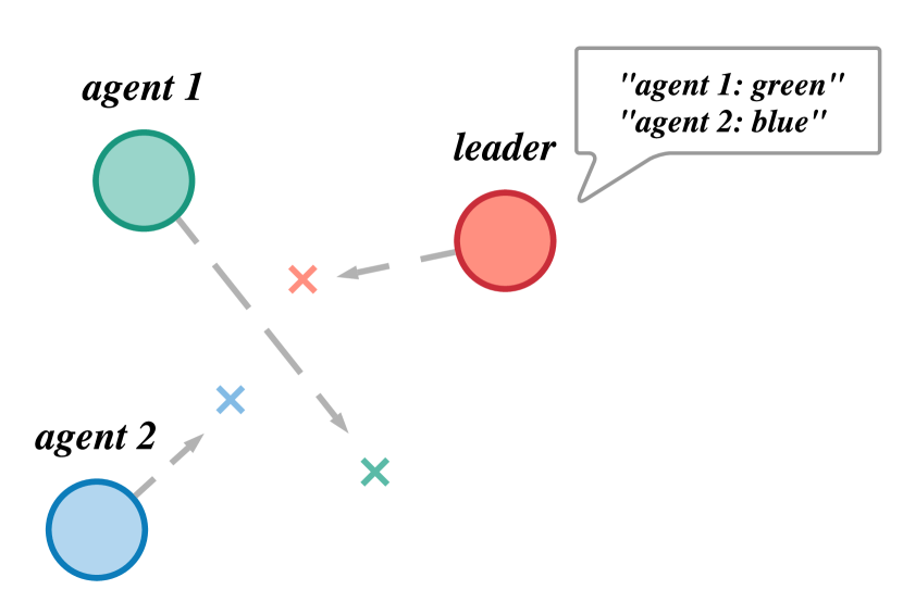
Figure 7: Cooperative scheduling task.

Cooperative scheduling.

scenario is described in Section 6, as shown in Figure 7. Agents are collectively rewarded based on the proximity of each agent to its corresponding landmark. There is one leader that knows the correspondence between agents and landmarks, the other two agents that need to know their corresponding landmarks via communication with the leader. The agents do not collide in this task. We implement the model-free algorithms with opponent modeling in this task.

Climb.

The agents have different preferences in two states. At state 1, agent 1 maximizes the reward by moving to the lower left landmark. By contrast, agent 2 can get different rewards by moving to both landmarks, computed as $\max(-2(a+0.5)^{2}-2(b+0.5)^{2},-(a-0.5)^{2}-(b-0.5)^{2})$. At state 2, the agents’ preferences change, agent 1 maximizes the reward by moving to the upper right landmark. By contrast, agent 2 can get different rewards by moving to both landmarks, computed as $\max(-(a+0.5)^{2}-(b+0.5)^{2},-2(a-0.5)^{2}-2(b-0.5)^{2})$.

Keep-away.

scenario with one agent, one adversary and two landmarks. The agent knows the target landmark and is rewarded based on the distance to the target landmark. The adversary is rewarded for preventing the agent from reaching the target landmark. The adversary does not know the correct landmark and must infer it from the movement of the agents.

Physical deception.

scenario with two agents, one adversary and two landmarks. The agents know the target landmark and are rewarded based on the minimum distance of any agent to the target landmark. The adversary does not know the target landmark and needs to reach the target landmark by following the agents. The agents are also rewarded by how well they deceive the adversary.

Predator-prey.

scenario with one prey (agent) and three predators (adversaries). The prey moves faster and is rewarded for running away from the three predators. The predators move slower and need to catch the prey through cooperation.

G.2 Cooperative Task Results

The Cooperative scheduling is set as a SECO task: (i) the agents do not collide, which makes the dynamics models prediction easier; (ii) the agents have heterogeneous action spaces, which make it more challenging for the opponent models to predict the opponents’ actions accurately. In the right subfigure of Figure 3, the sample efficiency refers to the amount of the interactions between the agents. For fair comparison, we implement the model-free baselines with opponent models in this experiment. Our methods AORPO and AORDPG reach the asymptotic performance with less agents’ interactions, which indicates high sample efficiency. Similar to the results for CESO tasks, our methods contribute to the more stable training process.

G.3 Competitive Task Results

We evaluate the sample efficiency of our method in the competitive environments on the Multi-Agent Particle Environment Lowe et al. [2017]. Three scenarios are included, i.e., 1) Keep-away scenario with an agent, an adversary and two landmarks, 2) Physical deception scenario with two agents, an adversary, and two landmarks, and 3) Predator-prey scenario with a prey (agent) and three predators (adversaries).

In these competitive tasks, we focus on the coordination within a team: the ego agent does not communicate with agents from other teams. While conducting the model rollouts, the ego agent $i$ communicates with only the agents of its own team, and samples actions of agents in the other teams with the opponent models.

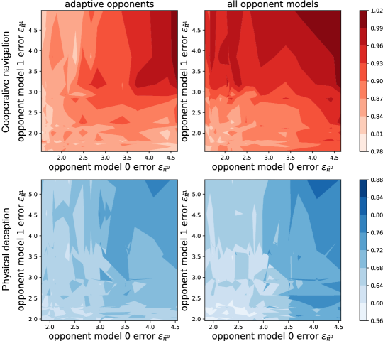
Figure 8: Model compounding errors in Cooperative navigation and Physical deception. The figures show the compounding errors (the dark color, the higher error) using different opponent model usages with opponent models that have different errors.

Experiment Protocol.

Each bar in Figure 9 shows the $[0,1]$ normalized agent reward score ($\textit{agent~{}reward}-\textit{adversary~{}reward}$). The higher score, the better for the agent. All the results are produced by evaluating every task 30 times with different random seeds.

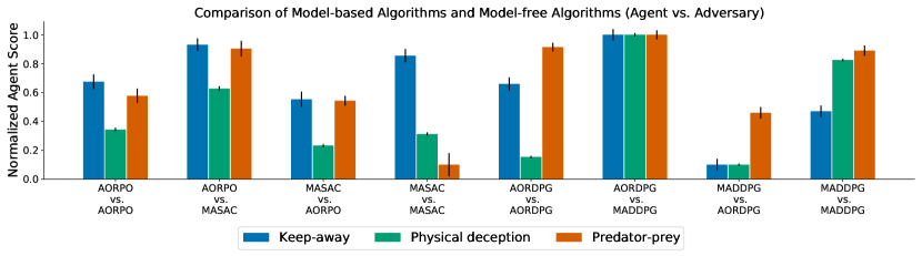
Figure 9: Performance comparison on the competition environments in Multi-Agent Particle Environment. Each bar shows the $[0,1]$ normalized agent score (agent reward minus adversary reward).

Since the choice of the base model-free algorithms affects the final performance in the competitive tasks, we compare AORPO and AORDPG with MASAC and MADDPG, respectively, following the evaluation protocol in Lowe et al. Lowe et al. [2017]. The comparison results are shown in Figure 9. We find that AORPO gets higher agent scores (agent reward minus adversary reward) than MASAC does when competing with the same rivals and that AORDPG outperforms MADDPG similarly.

More Detailed Performance.

The rows are the algorithms that used by the adversaries, and the columns are the ones used by the agents, i.e., the score of each entry corresponds to the performance of the column algorithm. Results are in Table 3 and 4.

(a) Results of Keep-away.

Algorithms	MASAC	AORPO
MASAC	-6.68	-6.28
AORPO	-8.31	-7.65

(b) Results of Physical deception.

Algorithms	MASAC	AORPO
MASAC	19.64	32.49
AORPO	16.36	20.89

(c) Results of Predator prey.

Algorithms	MASAC	AORPO
MASAC	-74.93	-25.69
AORPO	-47.79	-45.70

Table 3: Results of AORPO vs.MASAC.

(a) Results of Keep-away.

Algorithms	MADDPG	AORDPG
MADDPG	40.60	47.72
AORDPG	10.93	13.12

(b) Results of Physical deception.

Algorithms	MADDPG	AORDPG
MADDPG	-8.75	-5.91
AORDPG	-10.75	-7.73

(c) Results of Predator prey.

Algorithms	MADDPG	AORDPG
MADDPG	-26.53	-19.83
AORDPG	-52.89	-25.04

Table 4: Results of AORDPG vs. MADDPG.

G.4 Comparison with Other Model-based Algorithms

We compare our algorithm AORPO with the method called multi-agent RL with multi-step generative models (MAMSGM) as proposed by Krupnik et al. [2019]. We implement MAMSGM in the online form, which means that the method updates the models and collects data by planning the trajectories using the models. The experiments are conducted in the Predator prey scenario. The results are shown in Table 5, the meanings of the tables are the same as the ones in Appendix G.3, i.e., the score of each entry corresponds to the performance of the column algorithm.

(a) Results in Keep-away.

Algorithms	MAMSGM	AORPO
MAMSGM	-61.31	44.1
AORPO	-107.9	-7.65

(b) Results in Physical deception.

Algorithms	MAMSGM	AORPO
MAMSGM	134.3	221.44
AORPO	2.65	20.89

(c) Results in Predator prey.

Algorithms	MAMSGM	AORPO
MAMSGM	-69.03	-3.26
AORPO	-357.9	-45.69

Table 5: Comparison between AORPO and MAMSGM.

G.5 Model Error Analysis

In Figure 5, we have shown the relationship between the model compounding error and the interactions numbers of different rollout schemes. Further, we investigate that the adaptive opponent-wise rollout method can reduce the model compounding error with diverse opponent models. As shown in Figure 8, using opponent models with different performance, the adaptive opponent model selection reduces the model compounding errors generally.

G.6 More Analysis on Adaptive Opponent-wise Rollout

There are at least two feasible implementations of adaptive opponent-wise rollout schemes, namely simu-to-real rollout and real-to-simu rollout, as illustrated in Figure 10. The one shown in Figure 2 is the simu-to-real rollout. In this section, we discuss the pros and cons of these two schemes.

Figure 10: Two feasible adaptive opponent-wise rollout schemes. (a) simu-to-real rollout: first use opponent models to simulate the actions, then call the opponent agents for real actions; (b) real-to-simu rollout: first call the opponent agents for real actions, then use opponent models to simulate more actions.

We first analyze the difference of the state distance between these two alternatives. For simplicity, we consider the situation that there are only two opponents, and without loss of generality we assume the total branched rollout length using the opponent model $\hat{\pi}^{1}$ with small error is $k$ and the length of the other opponent model $\hat{\pi}^{2}$ performed rollout is $l$. We now briefly derive the state distance in the $k$ steps between the adaptive opponent-wise rollout and the scheme of using both real opponents in the dynamics model according to Extended Lemma C.2. For simu-to-real rollout, the state distance of the $k$ steps is bounded by $\sum_{t=1}^{k}t(\epsilon^{1}_{\hat{\pi}}+\epsilon^{2}_{\hat{\pi}})+l(k-l)(\epsilon^{1}_{\hat{\pi}}+\epsilon^{2}_{\hat{\pi}})+\sum_{t=l+1}^{k}(t-l)\epsilon^{1}_{\hat{\pi}}$ (the discount factor $\gamma$ is omitted for simplicity). And for real-to-simu rollout, the state distance of the $k$ steps is bounded by $\sum_{t=1}^{k-l}t\epsilon^{1}_{\hat{\pi}}+l(k-l)\epsilon^{1}_{\hat{\pi}}+\sum_{t=k-l+1}^{k}(t-k+l)(\epsilon^{1}_{\hat{\pi}}+\epsilon^{2}_{\hat{\pi}})$. By comparison, we find that the state distance in the $k$ steps of simu-to-real is larger than that of real-to-simu by $l(k-l)\epsilon^{2}_{\hat{\pi}}$, which means simu-to-real will compound more errors. This is easy to understand since in real-to-simu at first no error of the opponent model $\hat{\pi}^{2}$ is induced and thus will not be compound later.

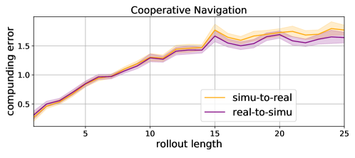
Figure 11: Model compounding errors and ratios for two rollout schemes.

Figure 11 shows the results in Cooperative communication scenario. We can see that the real-to-simu rollout scheme achieves lower compounding error than simu-to-real scheme for long rollout (when $k>15$) but the model compounding errors are almost the same for short rollout (when $k<15$). When $k=10$, the compounding errors are almost the same, while the contribution ratio of compounding error from opponent models from simu-to-real scheme is smaller than that from real-to-simu scheme. Furthermore, as shown in Figure 12 and Figure 13, the simu-to-real scheme actually achieves higher sample efficiency than real-to-simu scheme, for both $k=10$ and $k=20$, which looks counter-intuitive.

Figure 12: Effectiveness w.r.t. interactions, using fixed learned dynamics model and $k=20$.

Figure 13: The average episode reward performance for two rollout schemes, using $k=10$.

It may be counter-intuitive in the single-agent setting, while the situation is different in the multi-agent setting. We now provide the following detailed explanations for above observations. Although real-to-simu achieves less compounding error theoretically and empirically, yet the simulated rollouts generated by simu-to-real are more useful for policy training. If adopting the real-to-simu scheme, opponent models are exploited at the end when the error has been large already. In this situation, the dynamics model transits to useless states, and the opponent models provide unrealistic actions, which is of no use for ego policy training. Differently, if adopting the simu-to-real scheme, opponent models are exploited at the begging when the error is not large, and even if the error may be larger than in real-to-simu at the end, real opponents are used at this time, which at least guides the ego agent how to interact with others at these new states.

We think such an analysis requires a deeper investigation about the tigher compounding error bound w.r.t. the generalization error of the dynamics model and the opponent models, which deserves a thorough research work in the future.

References

• Bertsekas [2012] Dimitri P Bertsekas. Weighted sup-norm contractions in dynamic programming: A review and some new applications. Dept. Elect. Eng. Comput. Sci., Massachusetts Inst. Technol., Cambridge, MA, USA, Tech. Rep. LIDS-P-2884, 2012.
• Chua et al. [2018] Kurtland Chua, Roberto Calandra, Rowan McAllister, and Sergey Levine. Deep reinforcement learning in a handful of trials using probabilistic dynamics models. In NeurIPS, 2018.
• Clavera et al. [2020] Ignasi Clavera, Yao Fu, and Pieter Abbeel. Model-augmented actor-critic: Backpropagating through paths. In ICLR, 2020.
• Du and Ding [2020] Wei Du and Shifei Ding. A survey on multi-agent deep reinforcement learning: from the perspective of challenges and applications. Artificial Intelligence Review, 2020.
• Foerster et al. [2018] Jakob Foerster, Richard Y Chen, Maruan Al-Shedivat, Shimon Whiteson, Pieter Abbeel, and Igor Mordatch. Learning with opponent-learning awareness. In AAMAS. AAMAS, 2018.
• Haarnoja et al. [2018] Tuomas Haarnoja, Aurick Zhou, Kristian Hartikainen, George Tucker, Sehoon Ha, Jie Tan, Vikash Kumar, Henry Zhu, Abhishek Gupta, Pieter Abbeel, et al. Soft actor-critic algorithms and applications. arXiv preprint arXiv:1812.05905, 2018.
• He et al. [2016] He He, Jordan Boyd-Graber, Kevin Kwok, and Hal Daumé III. Opponent modeling in deep reinforcement learning. In ICML, 2016.
• Hu and Wellman [2003] Junling Hu and Michael P Wellman. Nash q-learning for general-sum stochastic games. JMLR, (Nov), 2003.
• Iqbal and Sha [2019] Shariq Iqbal and Fei Sha. Actor-attention-critic for multi-agent reinforcement learning. In ICML. PMLR, 2019.
• Jaakkola et al. [1994] Tommi Jaakkola, Michael I Jordan, and Satinder P Singh. Convergence of stochastic iterative dynamic programming algorithms. 1994.
• Jang et al. [2016] Eric Jang, Shixiang Gu, and Ben Poole. Categorical reparameterization with gumbel-softmax. arXiv preprint arXiv:1611.01144, 2016.
• Janner et al. [2019] Michael Janner, Justin Fu, Marvin Zhang, and Sergey Levine. When to trust your model: Model-based policy optimization. arXiv preprint arXiv:1906.08253, 2019.
• Jin et al. [2018] Chi Jin, Zeyuan Allen-Zhu, Sebastien Bubeck, and Michael I Jordan. Is q-learning provably efficient? In NeurIPS, 2018.
• Kamra et al. [2020] Nitin Kamra, Hao Zhu, Dweep Trivedi, Ming Zhang, and Yan Liu. Multi-agent trajectory prediction with fuzzy query attention. arXiv preprint arXiv:2010.15891, 2020.
• Kamthe and Deisenroth [2018] Sanket Kamthe and Marc Deisenroth. Data-efficient reinforcement learning with probabilistic model predictive control. In AISTATS, 2018.
• Krupnik et al. [2019] Orr Krupnik, Igor Mordatch, and Aviv Tamar. Multi agent reinforcement learning with multi-step generative models. arXiv preprint arXiv:1901.10251, 2019.
• Lakshminarayanan et al. [2017] Balaji Lakshminarayanan, Alexander Pritzel, and Charles Blundell. Simple and scalable predictive uncertainty estimation using deep ensembles. In NeurIPS, 2017.
• Li et al. [2020] Jiachen Li, Fan Yang, Masayoshi Tomizuka, and Chiho Choi. Evolvegraph: Multi-agent trajectory prediction with dynamic relational reasoning. NeurIPS, 2020.
• Lowe et al. [2017] Ryan Lowe, Yi Wu, Aviv Tamar, Jean Harb, OpenAI Pieter Abbeel, and Igor Mordatch. Multi-agent actor-critic for mixed cooperative-competitive environments. In NeurIPS, 2017.
• Luo et al. [2019] Yuping Luo, Huazhe Xu, Yuanzhi Li, Yuandong Tian, Trevor Darrell, and Tengyu Ma. Algorithmic framework for model-based deep reinforcement learning with theoretical guarantees. In ICLR, 2019.
• Nagabandi et al. [2018] Anusha Nagabandi, Gregory Kahn, Ronald S Fearing, and Sergey Levine. Neural network dynamics for model-based deep reinforcement learning with model-free fine-tuning. In ICRA. IEEE, 2018.
• Park et al. [2019] Young Joon Park, Yoon Sang Cho, and Seoung Bum Kim. Multi-agent reinforcement learning with approximate model learning for competitive games. PloS one, (9), 2019.
• Qu et al. [2019] Chao Qu, Shie Mannor, Huan Xu, Yuan Qi, Le Song, and Junwu Xiong. Value propagation for decentralized networked deep multi-agent reinforcement learning. In NeurIPS, 2019.
• Ramachandran et al. [2017] Prajit Ramachandran, Barret Zoph, and Quoc V Le. Searching for activation functions. arXiv preprint arXiv:1710.05941, 2017.
• Ryu et al. [2020] Heechang Ryu, Hayong Shin, and Jinkyoo Park. Multi-agent actor-critic with hierarchical graph attention network. In AAAI, 2020.
• Shapley [1953] Lloyd S Shapley. Stochastic games. PNAS, (10), 1953.
• Sutton [1990] Richard S Sutton. Integrated architectures for learning, planning, and reacting based on approximating dynamic programming. In Machine learning proceedings 1990. Elsevier, 1990.
• Szepesvári and Littman [1999] Csaba Szepesvári and Michael L Littman. A unified analysis of value-function-based reinforcement-learning algorithms. Neural computation, (8), 1999.
• Tian et al. [2019] Zheng Tian, Ying Wen, Zhichen Gong, Faiz Punakkath, Shihao Zou, and Jun Wang. A regularized opponent model with maximum entropy objective. IJCAI, 2019.
• Tian et al. [2020] Zheng Tian, Shihao Zou, Ian Davies, Tim Warr, Lisheng Wu, Haitham Bou-Ammar, and Jun Wang. Learning to communicate implicitly by actions. In AAAI, 2020.
• Wang et al. [2019] Tingwu Wang, Xuchan Bao, Ignasi Clavera, Jerrick Hoang, Yeming Wen, Eric Langlois, Shunshi Zhang, Guodong Zhang, Pieter Abbeel, and Jimmy Ba. Benchmarking model-based reinforcement learning. arXiv preprint arXiv:1907.02057, 2019.
• Wei et al. [2018] Ermo Wei, Drew Wicke, David Freelan, and Sean Luke. Multiagent soft q-learning. In AAAI, 2018.
• Wen et al. [2019] Ying Wen, Yaodong Yang, Rui Luo, Jun Wang, and W Pan. Probabilistic recursive reasoning for multi-agent reinforcement learning. In ICLR, 2019.
• Whiteson [2018] Shimon Whiteson. Qmix: Monotonic value function factorisation for deep multi- agent reinforcement learning. ICML, 2018.
• Yang et al. [2018] Yaodong Yang, Rui Luo, Minne Li, Ming Zhou, Weinan Zhang, and Jun Wang. Mean field multi-agent reinforcement learning. arXiv preprint arXiv:1802.05438, 2018.
• Zhang et al. [2018] Kaiqing Zhang, Zhuoran Yang, Han Liu, Tong Zhang, et al. Fully decentralized multi-agent reinforcement learning with networked agents. PMLR, 2018.