Dalitz plot studies of $D^{0}\to K^{0}_{S}K^{+}K^{-}$ decays in a factorization approach

Abstract

The BABAR Collaboration data of the $D^{0}\to K^{0}_{S}K^{+}K^{-}$ process are analyzed within a quasi-two-body factorization framework. Starting from the weak effective Hamiltonian, one has to evaluate matrix elements of $D^{0}$ transitions to two kaons for the tree amplitudes and the transitions between one kaon and two kaons for the annihilation ones ($W$-exchange). In earlier studies, assuming these transitions to proceed through the dominant intermediate resonances, we approximated them as being proportional to the kaon form factors. Here, to obtain a good fit, one has to multiply the scalar-kaon form factors, derived from unitary relativistic coupled-channel models or in a dispersion relation approach, by phenomenological energy-dependent functions. The final state kaon-kaon interactions in the $S$-, $P$- and $D$- waves are taken into account. All $S$-wave channels are treated in a unitary way. In other respects, it is shown in a model-independent manner that the $K^{+}K^{-}$ and $\bar{K}^{0}K^{+}$ $S$-wave effective mass squared distributions, corrected for phase space, are significantly different. At variance with the BABAR analysis, it means that the $f_{0}(980)$ resonance must be included in the phenomenological analysis of the $D^{0}\to K^{0}_{S}K^{+}K^{-}$ data. The best fit described in the main text has 19 free parameters and indicates i) the dominance of annihilation amplitudes, ii) a large dominance of the $f_{0}(980)$ meson in the near threshold $K^{+}K^{-}$ invariant mass distribution, and iii) a sizable branching fraction to the $[\rho(770)^{+}+\rho(1450)^{+}+\rho(1700)^{+}]K_{S}^{0}$ final states. A first appendix provides an update of the determination of the isoscalar-scalar meson-meson amplitudes based on an enlarged set of data embodying new precise low energy $\pi\pi$ data. A second appendix proposes two alternative fits using the scalar-kaon form factors calculated from the Muskhelishvili-Omnès dispersion relation approach. These fits have $\chi^{2}$ quite close to that of the best fit but they show important contributions from both the $f_{0}$ and $a_{0}^{0}$ mesons and a weaker role of the $\rho^{+}$ mesons.

I Introduction

Measurements of the $D^{0}$-$\overline{D}^{0}$ mixing parameters, through Dalitz-plot time dependent amplitude analyses of the weak process $D^{0}\to K^{0}_{S}K^{+}K^{-}$, have been performed by the Belle Zupanc2009 and BABAR collaborations B10 . Such studies could help in the understanding of the origin of mixing and may indicate the presence of new physics contribution. As predicted by the standard model in the charm sector, the violation of the CP symmetry should be small for these $D^{0}$ decays. In Refs. Zupanc2009 ; B10 the description of the $D^{0}\to K^{0}_{S}K^{+}K^{-}$ decay amplitude has been performed using the isobar model developed in B5 , extended in Aubert2008 and B10 ; supmaPRL105 . The isobar model has also been applied in the experimental analysis based on the data taken from the BESIII experiment Weidenkaff ; Ablikim2006.02800 .

The Cabibbo-Kobayashi-Maskawa (CKM) angle $\gamma$ (or $\phi_{3}$) has been evaluated from the analyses of the $B^{\pm}\to D^{0}K^{\pm}$, with $D^{0}\to K^{0}_{S}\pi^{+}\pi^{-}$ and $D^{0}\to K^{0}_{S}K^{+}K^{-}$decays SanchezPRL105121801 ; Poluektov2010 ; J.P.Lees_PRD87_052015_BABAR ; LHCbNP2014 . This angle can be also measured using some knowledge on the strong-phase difference between $D^{0}$ and $\bar{D}^{0}\to K^{0}_{S}K^{+}K^{-}$ decay amplitudes obtained by the CLEO Collaboration J.Libby_PRD82_CLEO . This method has been used by the Belle H.Aihara_Belle2012 , LHCb R.Aaij_JHEP2018 and BESIII BES2007 collaborations.

A good knowledge of the final state meson interactions in the $D^{0}\to K^{0}_{S}K^{+}K^{-}$ decays is important to reduce the uncertainties in the determination of the $D^{0}$-$\overline{D}^{0}$ mixing parameters and of the CKM angle $\gamma$. The structures seen in the Dalitz plot spectra point out to the complexity of these final state strong interactions. Their studies can provide a better understanding of the strange meson interactions and of the $D^{0}$ decay mechanism into $K^{0}_{S}K^{+}K^{-}$.

The experimental analyses like that of Ref. B10 rely mainly upon the use of the isobar model. For a given reaction, this model has basically two fitted parameters for each part of the decay amplitude. In this approach one can take into account many existing resonances coupled to the interacting pairs of mesons. In Refs. B10 ; supmaPRL105 , the authors introduce explicitly eight resonances $a_{0}(980)^{0}$ , $a_{0}(980)^{+}$ , $a_{0}(980)^{-}$ , $\phi(1020)$ , $f_{2}(1270)$ , $f_{0}(1370)$ , $a_{0}(1450)^{0}$ , $a_{0}(1450)^{+}$ . Their analysis rely on 17 free parameters. However, the decay amplitudes are not unitary and unitarity is not preserved in the three-body decay channels; it is also violated in the two-body subchannels. Furthermore, it is difficult to differentiate the $S$-wave amplitudes from the nonresonant background terms. Their interferences are noteworthy and then some two-body branching fractions, extracted from the data, could be unreliable. One of the difficulty in the experimental analyses based on the isobar model is the choice of the resonances needed to reach a good agreement with the Dalitz plot data. In Ref. Aubert2008 the BABAR collaboration authors have added the scalar $a_{0}(1450)$ to their model developed in 2005 B5 . In the recent BESIII analysis Ablikim2006.02800 the Dalitz plot is described with six resonances: $a_{0}(980)^{0}$ , $a_{0}(980)^{+}$ , $\phi(1020)$ , $a_{2}(1320)^{+}$ , $a_{2}(1320)^{-}$ , $a_{0}(1450)^{-}$.

Extending our previous work on the $D^{0}\to K^{0}_{S}\pi^{+}\pi^{-}$ decays JPD_PRD89 , we analyze, in the quasi-two-body factorization framework, the $D^{0}\to K^{0}_{S}K^{+}K^{-}$ data provided by the BABAR collaboration B10 . As in our earlier studies, we assume that two of the three final-state mesons form a single state which originates from a quark-antiquark, $q\bar{q}$, pair and then apply the factorization procedure to these quasi-two-body final states. Starting from the weak effective Hamiltonian, we derive tree and annihilation ($W$-meson exchange) amplitudes both being either Cabibbo favored (CF) with $c\to s\bar{d}u$ transition or doubly Cabibbo suppressed (DCS) with $c\to du\bar{s}$ transition.

In the factorization approach, the CF and DCS amplitudes are expressed as superpositions of appropriate effective coefficients and two products of two transition matrix elements. The kaon form factors do not appear explicitly except the isovector ones that enter in only one term of the CF tree amplitude. In all other terms of our amplitudes, one has to evaluate either, for the tree ones, the matrix elements of $D^{0}$ transitions to two-kaon states or, for the annihilation ones, the transitions between one kaon and two kaon-states. Similarly to previous studies Boito , assuming these transitions to proceed through the dominant intermediate resonances, we have approximated them as being proportional to the isoscalar or isovector kaon form factors.

Taking advantage of the coupling between the $\pi\pi$ and the $K\overline{K}$ channels and extending the derivation of the unitary isoscalar-scalar pion form factor DedonderPol to that of the kaon one, two of the present authors (L. L. and R. K.) together with two collaborators, have recently studied, in the quasi-two-body QCD factorization approach, the $B^{\pm}\to K^{+}K^{-}K^{\pm}$ decays PLB699_102 ; KKK . These $S$-wave form factors are derived using a unitary relativistic three coupled-channel model including $\pi\pi$, $K\bar{K}$ and effective $(2\pi)(2\pi)$ interactions together with chiral symmetry constraints. They include the contributions of the $f_{0}(980)$ and $f_{0}(1400)$ resonances and require the knowledge of the isoscalar-scalar meson-meson amplitudes from the two kaon threshold to energies above the $D^{0}$ mass. The parameters of these amplitudes derived in the late nineties by three of us (R. K., L. L. and B. L.) KLL ; EPJ have been updated using new precise low energy $\pi\pi$ data together with an enlarged set of data as is shown in Appendix A.

The calculation requires also the knowledge of a contribution proportional to the isovector-scalar form factor; it is represented by a function calculated from a unitary model with relativistic two-coupled channel $\pi\eta$ and $K\bar{K}$ equations based on the two-channel model of the $a_{0}(980)$ and $a_{0}(1450)$ resonances built in AFLL ; AFLL2 .

The vector form factors have been calculated using vector dominance, quark model assumptions and isospin symmetry in Ref. Bruch2005 . They receive contributions from the vector mesons: $\rho(770)$, $\rho(1450)$, $\rho(1700)$, $\omega(782)$, $\omega(1420)$, $\omega(1850)$, $\phi(1020)$ and $\phi(1680)$. The isoscalar-tensor amplitude, saturated by the $f_{2}(1270)$, is described by a relativistic Breit-Wigner term. The isovector-tensor resonance $a_{2}(1320)$ has a mass close to that of the $f_{2}(1270)$. If the contribution of these tensor mesons are described by relativistic Breit-Wigner components, it is difficult to disentangle them because of the degeneracy in their masses, widths and partial decay widths into $K\overline{K}$ PDG2020 . Consequently, as in Ref. B10 , we consider only the $f_{2}(1270)$ to represent the $D$ wave. It is an “effective” $f_{2}(1270)$ which takes into account both tensor mesons.

In the present approach, a best fit is achieved in which the data are reproduced with amplitudes that are optimized notably by adjusting the isoscalar- and isovector-scalar form factors. It is interesting then to see what could be the outcome of a model based, for instance, on the scalar form factors calculated from the Muskhelishvili-Omnès dispersion relation approach MO ; Moussallam_2000 ; Moussallam_2019 ; Bachir2015 . As in our best fit model ($\chi^{2}/ndf=1.25$), we have to introduce energy dependent phenomenological functions multiplying the scalar form factors to obtain two fits with almost as good $\chi^{2}/ndf$. Branching fractions of these two alternative models are compared to those of our best fit model.

The paper is organized as follows. A full derivation of the $D^{0}\to K^{0}_{S}K^{+}K^{-}$ decay amplitude, in the framework of the quasi-two-body factorization approach is given in Sec. II. Based only on the experimental data of the BABAR Collaboration B10 and without any model assumptions, we show in Sec. III that the $f_{0}(980)$ contribution, at variance with the BABAR analysis, has to be included in the decay amplitude. Section IV presents the result of our best fit to the Dalitz plot data sample of Ref. B10 . Some discussion and concluding remarks can be found in Sec. V. Appendix A presents the update of the description of the $\pi\pi$, $\bar{K}K$ and effective $(2\pi)(2\pi)$ S-wave isospin zero scattering amplitudes. Two alternative models for the $D^{0}\to K^{0}_{S}K^{+}K^{-}$ decay amplitude, using kaon scalar-form factors derived from the dispersion relation approach, are presented in Appendix B.

II The $D^{0}\to K^{0}_{S}K^{+}K^{-}$ decay amplitudes in a factorization framework

The decay amplitudes for the $D^{0}\to K^{0}_{S}K^{+}K^{-}$ process can be evaluated as matrix elements of the effective weak Hamiltonian Buchalla1996

$$H_{eff}=\frac{G_{F}}{\sqrt{2}}V_{CKM}\Big{[}C_{1}(\mu)O_{1}(\mu)+C_{2}(\mu)O_{2}(\mu)\Big{]}+h.c.,$$ (1)

where the coefficients $V_{CKM}$ are given in terms of Cabibbo-Kobayashi-Maskawa quark-mixing matrix elements and $G_{F}$ denotes the Fermi coupling constant. The $C_{i}(\mu)$ are the Wilson coefficients of the four-quark operators $O_{i}(\mu)$ at a renormalization scale $\mu$, chosen to be equal to the $c$-quark mass $m_{c}$. The left-handed current-current operators $O_{1,2}(\mu)$ arise from $W$-boson exchange.

The transition matrix elements that occur in the present work require two specific values of the $V_{CKM}$ coupling matrix elements JPD_PRD89 :

$$\Lambda_{1}\equiv V^{*}_{cs}V_{ud}=1-\lambda^{2}\hskip 28.45274pt{\rm and}\hskip 28.45274pt\Lambda_{2}\equiv V^{*}_{cd}V_{us}=-\lambda^{2},$$ (2)

where $\lambda$ is the sine of the Cabibbo angle and where $\Lambda_{1}$ is associated to Cabibbo favored (CF) transitions while $\Lambda_{2}$ is associated to doubly Cabibbo suppressed (DCS) amplitudes. The amplitudes are functions of the Mandelstam invariants

$$s_{\pm}=m_{\pm}^{2}=(p_{0}+p_{\pm})^{2},\hskip 56.9055pts_{0}=m_{0}^{2}=(p_{+}+p_{-})^{2},$$ (3)

where $p_{0}$, $p_{+}$ and $p_{-}$ are the four-momenta of the $K_{S}^{0}$, $K^{+}$ and $K^{-}$ mesons, respectively. Energy-momentum conservation implies

$$p_{D^{0}}=p_{0}+p_{+}+p_{-}\hskip 28.45274pt{\rm and}\hskip 28.45274pts_{0}+s_{+}+s_{-}=m_{D^{0}}^{2}+m_{K^{0}}^{2}+2m_{K}^{2},$$ (4)

where $p_{D^{0}}$ is the $D^{0}$ four-momentum and $m_{D^{0}}=1864.83$ MeV, $m_{K^{0}}=497.611$ MeV and $m_{K}=493.677$ MeV denote the $D^{0}$, $K^{0}$ and charged kaon masses (Ref. PDG2020 ).

II.1 Tree and annihilation CF and DCS amplitudes

The full amplitude is the superposition of two tree CF and DCS amplitudes, $T^{CF}(s_{0},s_{-},s_{+})$ and $T^{DCS}(s_{0},s_{-},s_{+})$ and of two annihilation (i.e., exchange of W meson between the $c$ and $\overline{u}$ quarks of the $D^{0}$) CF and DCS amplitudes, $A^{CF}(s_{0},s_{-},s_{+})$ and $A^{DCS}(s_{0},s_{-},s_{+})$. Thus, one writes the full amplitude as

$$\mathcal{M}(s_{0},s_{-},s_{+}) = \left\langle K^{0}_{S}(p_{0})\ K^{+}(p_{+}){K^{-}}(p_{-})|H_{eff}|D^{0}(p_{D^{0}})\right\rangle$$ (5)

$$= T^{CF}(s_{0},s_{-},s_{+})+T^{DCS}(s_{0},s_{-},s_{+})+A^{CF}(s_{0},s_{-},s_{+})+A^{DCS}(s_{0},s_{-},s_{+}).$$

Although the three variables $s_{0},s_{-},s_{+}$ appear as arguments of the amplitudes, all amplitudes depend only on two of them because of the relation (4).

Figure 1: Tree diagrams for Cabibbo favored amplitudes proportional to $\Lambda_{1}\ a_{1}$ with $K^{-}\left[\overline{K}^{0}\ K^{+}\right]$ final states

Assuming that the factorization approach Beneke2003 ; BurasNPB434_606 ; Buchalla1996 ; AliPRD58 holds, the diagram illustrated in Fig. 1 is proportional to $\Lambda_{1}a_{1}(m_{c})$ with quasi-two-body $K^{-}[\overline{K}^{0}K^{+}]_{L}^{I=1}$ final states and the diagram in Fig. 2, proportional to $\Lambda_{1}a_{2}(m_{c})$ with quasi-two-body $\overline{K}^{0}[K^{+}K^{-}]_{L}^{I}$ with angular momentum $L=S,P,D$ and isospin $I=0,1$ states, yield the tree CF amplitude $T^{CF}(s_{0},s_{-},s_{+})$ which reads, with $|0\rangle$ denoting the vacuum state,

$$T^{CF}(s_{0},s_{-},s_{+})\! \simeq \frac{G_{F}}{2}\Lambda_{1}\!\sum_{L={S,P,D}}\left\{a_{1}(m_{c})\langle\left[\overline{K}^{0}(p_{0})\ K^{+}(p_{+})\right]_{L}^{I=1}|(\overline{u}\ d)_{V-A}|0\rangle\langle K^{-}(p_{-})|(\overline{s}\ c)_{V-A}|D^{0}(p_{D^{0}})\right.\rangle$$ (6)

$$+ \left.a_{2}(m_{c})\sum_{I={0,1}}\ \langle\overline{K}^{0}(p_{0})|(\overline{s}\ d)_{V-A}|0\rangle\langle[K^{+}(p_{+}){K^{-}}(p_{-})]_{L,u}^{I}|(\overline{u}\ c)_{V-A}|D^{0}(p_{D^{0}})\rangle\right\}$$

$$= \sum_{L={S,P,D}}\!\!\left[T^{CF}_{[\overline{K}^{0}K^{+}]_{L}^{1}K^{-}}(s_{0},s_{-},s_{+})+T^{CF}_{\overline{K}^{0}[K^{+}K^{-}]_{L,u}^{0}}(s_{0},s_{-},s_{+})+T^{CF}_{\overline{K}^{0}[K^{+}K^{-}]_{L,u}^{1}}(s_{0},s_{-},s_{+})\right]$$

$$= T^{CF}_{[\overline{K}^{0}K^{+}]^{1}K^{-}}(s_{0},s_{-},s_{+})+\sum_{I=0,1}T^{CF}_{\overline{K}^{0}[K^{+}K^{-}]_{u}^{I}}(s_{0},s_{-},s_{+}).$$

The short hand notation of the last line of Eq. (6) implies the L summation. It will be used wherever necessary. In the case of the creation of a $K^{+}K^{-}$ pair we indicate by a subscript $q$ the $q\overline{q}$ pair from which it originates (here a $u\overline{u}$ one, as seen in Fig. 2). We shall therefore use the notation $[K^{+}K^{-}]_{L,q}^{I}$ and/or $[K^{+}K^{-}]_{q}^{I}$ whenever necessary. We have also introduced the short-hand notation

$$(\overline{q}\ q)_{V-A}=\overline{q}\gamma\ (1-\gamma_{5})\ q$$ (7)

which will be used throughout the text ($\gamma$ and $\gamma_{5}$ are Dirac’s matrices). In deriving Eq. (6) small $CP$ violation effects in $K^{0}_{S}$ decays are neglected and we use

$$|K^{0}_{S}\rangle\approx\frac{1}{\sqrt{2}}\ \left(|K^{0}\rangle+|\overline{K}^{0}\rangle\right).$$ (8)

At leading order in the strong coupling constant $\alpha_{S}$, the effective QCD factorization coefficients $a_{1}(m_{c})$ and $a_{2}(m_{c})$ are expressed as

$$a_{1}(m_{c})=C_{1}(m_{c})+\frac{C_{2}(m_{c})}{N_{C}},\hskip 28.45274pta_{2}(m_{c})=C_{2}(m_{c})+\frac{C_{1}(m_{c})}{N_{C}},$$ (9)

where $N_{C}=3$ is the number of colors. Higher order vertex and hard scattering corrections are not discussed in the present work and we introduce effective values for these coefficients. From now on, the simplified notation $a_{1}\equiv a_{1}(m_{c})$ and $a_{2}\equiv a_{2}(m_{c})$ will be used. As in Ref. JPD_PRD89 , we take $a_{1}=1.1$ and $a_{2}=-0.5$.

Figure 2: Tree diagram for Cabibbo favored amplitudes proportional to $\Lambda_{1}a_{2}$ with $\overline{K}^{0}\ \left[K^{+}K^{-}\right]_{u}^{I=0,1}$ final states

Similarly, the DCS tree amplitudes illustrated in Figs. 3 and 4, yield the amplitude $T^{DCS}(s_{0},s_{-},s_{+})$

$$T^{DCS}(s_{0},s_{-},s_{+})\! \simeq \!\frac{G_{F}}{2}\ \Lambda_{2}\sum_{L={S,P,D}}\!\Big{\{}a_{1}\langle K^{+}(p_{+})|(\overline{u}\ s)_{V-A}|0\rangle\ \langle[K^{0}(p_{0})\ K^{-}(p_{-})]_{L}^{1}|(\overline{d}\ c)_{V-A}|D^{0}(p_{D^{0}})\rangle$$ (10)

$$+ a_{2}\sum_{I=0,1}\langle K^{0}(p_{0})|(\overline{d}\ s)_{V-A}|0\rangle\ \langle[K^{+}(p_{+})\ K^{-}(p_{-})]_{L,u}^{I}|(\overline{u}\ c)_{V-A}|D^{0}(p_{D^{0}})\rangle\Big{\}}$$

$$= \!\sum_{L={S,P,D}}\!\left[T^{DCS}_{K^{+}[{K}^{0}K^{-}]_{L}^{1}}(s_{0},s_{-},s_{+})+T^{DCS}_{{K}^{0}[K^{+}K^{-}]_{L,u}^{0}}(s_{0},s_{-},s_{+})+T^{DCS}_{{K}^{0}[K^{+}K^{-}]_{L,u}^{1}}(s_{0},s_{-},s_{+})\right]$$

$$= \!T^{DCS}_{K^{+}[{K}^{0}K^{-}]^{1}}(s_{0},s_{-},s_{+})\!+\sum_{I=0,1}T^{DCS}_{{K}^{0}[K^{+}K^{-}]_{u}^{I}}(s_{0},s_{-},s_{+}).$$

Figure 3: Tree diagram for doubly Cabibbo suppressed amplitudes for $K^{+}\left[{K}^{0}K^{-}\right]^{I=1}$ final states

Figure 4: Tree diagram for doubly Cabibbo suppressed amplitudes for ${K}^{0}\left[K^{+}\ K^{-}\right]_{u}^{I=0,1}$ final states

A similar derivation goes for the CF annihilation amplitudes illustrated by the diagram of Fig. 5, $A^{CF}(s_{0},s_{-},s_{+})$, so that one has

$$A^{CF}(s_{0},s_{-},s_{+}) \simeq \frac{G_{F}}{2}\ \Lambda_{1}\ a_{2}\sum_{L={S,P,D}}\Big{\{}\sum_{I={0,1}}\langle\overline{K}^{0}(p_{0})[K^{-}(p_{-})K^{+}(p_{+})]_{L,s}^{I}|(\overline{s}\ d)_{V-A}|0\rangle$$ (11)

$$+ \langle K^{-}(p_{+})[\overline{K}^{0}(p_{0})K^{+}(p_{-})]_{L}^{1}|(\overline{s}\ d)_{V-A}|0\rangle\Big{\}}\ \langle 0|(\overline{c}\ u)_{V-A}|D^{0}(p_{D^{0}})\rangle$$

$$= \sum_{L={S,P,D}}\Big{[}A^{CF}_{K^{-}[\overline{K}^{0}K^{+}]_{L}^{1}}(s_{0},s_{-},s_{+})+A^{CF}_{\overline{K}^{0}[K^{+}K^{-}]_{L,s}^{0}}(s_{0},s_{-},s_{+})\Big{]}$$

$$= A^{CF}_{K^{-}[\overline{K}^{0}K^{+}]^{1}}(s_{0},s_{-},s_{+})+A^{CF}_{\overline{K}^{0}[K^{+}K^{-}]_{s}^{0}}(s_{0},s_{-},s_{+}).$$

Figure 5: Diagram for CF annihilation ($W$-exchange) amplitudes with $\overline{K}^{0}\ \left[K^{+}\ K^{-}\right]_{s}^{I=0}$ or $K^{-}[K^{+}\overline{K}^{0}]^{I=1}$ final states.

Figure 6: Diagram for DCS annihilation ($W$-exchange) amplitudes with ${K}^{0}\ \left[K^{+}\ K^{-}\right]_{s}^{I=0}$ or $K^{+}\left[K^{0}K^{-}\right]^{I=1}$ final states.

The corresponding DCS annihilation amplitudes, $A^{DCS}(s_{0},s_{-},s_{+})$, (see Fig. 6), are easily obtained from the CF amplitudes in Eq. (11)

$$A^{DCS}(s_{0},s_{-},s_{+}) \approx \frac{G_{F}}{2}\ \Lambda_{2}\ a_{2}\ \sum_{L={S,P,D}}\sum_{I=0,1}\Big{[}\langle[K^{-}(p_{-})K^{+}(p_{+})]_{L,s}^{I}{K}^{0}(p_{0})|(\overline{d}\ s)_{V-A}|0\rangle$$ (12)

$$+ \langle K^{+}(p_{+})[K^{0}(p_{0})K^{-}(p_{-})]_{L}^{1}|(\overline{d}\ s)_{V-A}|0\rangle\Big{]}\langle 0|(\overline{c}\ u)_{V-A}|D^{0}(p_{D^{0}})\rangle$$

$$= \sum_{L={S,P,D}}\Big{[}A^{DCS}_{K^{+}[K^{0}K^{-}]_{L}^{1}}(s_{0},s_{-},s_{+})+A^{DCS}_{K^{0}[K^{+}K^{-}]_{L,s}^{0}}(s_{0},s_{-},s_{+})\Big{]}$$

$$= A^{DCS}_{K^{+}[K^{0}K^{-}]^{1}}(s_{0},s_{-},s_{+})+A^{DCS}_{K^{0}[K^{+}K^{-}]_{s}^{0}}(s_{0},s_{-},s_{+}).$$

Let us now review in detail all the amplitudes that will have to be evaluated. We will follow closely the construction detailed in Ref. JPD_PRD89 .

II.2 Explicit tree amplitudes

In the following, starting from the expressions given in Eqs. (6) for the CF amplitudes and in (10) for the DCS ones, we will express the different three-body matrix elements entering in the amplitudes in terms of vertex functions noted $G_{R_{S,P,D}[\overline{K}^{0}K^{+}]^{1}}(s)$ in the case of a $[\overline{K}^{0}K^{+}]^{1}$ final state, $G_{R_{S,P,D}[{K}^{0}K^{-}]^{1}}(s)$ in the case of a $[{K}^{0}K^{-}]^{1}$ final state, and $G_{R_{S,P,D}[{K}^{+}K^{-}]_{q}^{0,1}}(s)$ in the case of a $[{K}^{+}K^{-}]_{q}^{0,1}$ final state. The vertex functions describe the decays into $K\overline{K}$ of the possibly present intermediate resonances $R_{S,P,D}$ which contribute to the process.

Further on, we will need to introduce transition form factors for which, as in Ref. JPD_PRD89 , we will assume isospin and charge conjugation symmetry so that the following equations arise:

$$F_{0}^{D^{0}a_{0}^{-}}(s) = \sqrt{2}\ F_{0}^{D^{0}a_{0}^{0}}(s),$$

$$F_{0}^{[{\overline{K}^{0}K^{+}}]^{1}}(s) = F_{0}^{[{{K}^{0}K^{-}}]^{1}}(s),$$

$$F_{1}^{\overline{K}^{0}K^{+}}(s) = -F_{1}^{{K}^{0}K^{-}}(s),$$

$$F_{0}^{K^{-}a_{0}^{+}}(m_{D^{0}}^{2}) = \sqrt{2}\ F_{0}^{K^{0}a_{0}^{0}}(m_{D^{0}}^{2}),$$

$$A_{0}^{D^{0}\rho^{-}}(s) = \sqrt{2}\ A_{0}^{D^{0}\rho^{0}}(s),$$

$$A_{0}^{\overline{K}^{0}\phi}(m_{D^{0}}^{2}) = A_{0}^{K^{0}\phi}(m_{D^{0}}^{2}).$$ (13)

In the above equations $F_{0}$ and $F_{1}$ denote scalar and vector transition form factors of two pseudoscalar mesons while $A_{0}$’s are transition form factors of pseudoscalar and vector mesons.

II.2.1 Scalar amplitudes

Following a derivation similar to that developped in Ref. JPD_PRD89 , the isoscalar-scalar CF amplitude associated to the $\overline{K}^{0}\ [K^{+}K^{-}]_{S,u}^{I}$ final states can be described by (see Fig. 2)

$$T^{CF}_{\overline{K}^{0}\ [K^{+}K^{-}]_{S,u}^{0}}(s_{0},s_{-},s_{+}) = -\frac{G_{F}}{2}\ \Lambda_{1}\ a_{2}\ \frac{f_{K^{0}}}{\sqrt{2}}\ (m_{D^{0}}^{2}-s_{0})\ \sum_{R_{S}}F_{0}^{D^{0}R_{S}[K^{+}K^{-}]_{u}^{0}}(m_{K^{0}}^{2})$$ (14)

$$\times \ G_{R_{S}[K^{+}K^{-}]_{u}^{0}}(s_{0})\ \langle R_{S}[K^{+}K^{-}]_{u}^{0}|u\overline{u}\rangle,$$

where $f_{K^{0}}$ is the $K^{0}$ decay constant and the sum over $R_{S}$ runs over the possibly contributing resonances in the isoscalar-scalar channel. It can be seen here that we have approximated the three-body matrix element $\langle[K^{+}(p_{+}){K^{-}}(p_{-})]_{S,u}^{0}|(\overline{u}\ c)_{V-A}|D^{0}(p_{D^{0}})\rangle$ entering Eq. (6) by the above sum over $R_{S}$. It thus includes the contributions of the $f_{0}(500)$, $f_{0}(980)$ and of the $f_{0}(1370)$ and $f_{0}(1500)$ resonances. The $D^{0}$ to $R_{S}$ transition form factor entering Eq. (14) could have a different value for each resonance $R_{S}$; here we can assume that its variation from one resonance to the other is small and we can choose for its value that of the transition to $f_{0}(980)$. Unless otherwise specified, by $f_{0}$ in $F_{0}^{D^{0}f_{0}}(m_{K^{0}}^{2})$ we mean $f_{0}(980)$. We may parametrize the sum over $R_{S}$ by introducing the isoscalar-scalar form factor, $\Gamma_{2}^{n*}(s_{0})$, where $n$ denotes a nonstrange quark pair and which can be built following the method discussed in Ref. DedonderPol . We then apply the following approximation

$$\sum_{R_{S}}F_{0}^{D^{0}R_{S}[K^{+}K^{-}]_{u}^{0}}(m_{K^{0}}^{2})\ G_{R_{S}[K^{+}K^{-}]_{u}^{0}}(s_{0})\ \langle R_{S}[K^{+}K^{-}]_{u}^{0}|u\overline{u}\rangle=\chi^{n}\ \frac{\Gamma_{2}^{n*}(s_{0})}{\sqrt{2}}\ F_{0}^{D^{0}f_{0}}(m_{K^{0}}^{2}),$$ (15)

where $\chi^{n}$ is a constant complex factor. Hence

$$T^{CF}_{\overline{K}^{0}\ [K^{+}K^{-}]_{S,u}^{0}}(s_{0},s_{-},s_{+})=-\frac{G_{F}}{2}\ \Lambda_{1}\ a_{2}\ \ f_{K^{0}}\ (m_{D^{0}}^{2}-s_{0})\ F_{0}^{D^{0}f_{0}}(m_{K^{0}}^{2})\ \frac{\chi^{n}}{2}\Gamma_{2}^{n*}(s_{0}).$$ (16)

The real transition form factor, $F_{0}^{D^{0}f_{0}}(m_{K^{0}}^{2})$, can be obtained from Ref. El-Bennich_PRD79 . This amplitude has to be associated with the corresponding isoscalar-scalar $K^{0}[K^{+}K^{-}]_{S,u}^{0}$ DCS amplitude (see Fig. 4) approximated by

$$T_{K^{0}[K^{+}K^{-}]_{S,u}^{0}}^{DCS}(s_{0},s_{-},s_{+})=\frac{\Lambda_{2}}{\Lambda_{1}}~{}T^{CF}_{\overline{K}^{0}\ [K^{+}K^{-}]_{S,u}^{0}}(s_{0},s_{-},s_{+})$$ (17)

Recombining the two amplitudes (16) and (17), we have

$$T_{1} = T_{K^{0}[K^{+}K^{-}]_{S,u}^{0}}^{CF}(s_{0},s_{-},s_{+})+T_{K^{0}[K^{+}K^{-}]_{S,u}^{0}}^{DCS}(s_{0},s_{-},s_{+})$$ (18)

$$= -\frac{G_{F}}{2}\ (\Lambda_{1}+\Lambda_{2})\ a_{2}\ f_{K^{0}}\ (m_{D^{0}}^{2}-s_{0})\ F_{0}^{D^{0}f_{0}}(m_{K^{0}}^{2})\ \frac{\chi^{n}}{2}\ \Gamma_{2}^{n*}(s_{0}).$$

We now turn to the three isovector-scalar tree amplitudes. The isovector-scalar $K^{+}[{K}^{0}K^{-}]_{S}$ DCS amplitude, associated to the $a_{0}(980)^{-}$ and $a_{0}(1450)^{-}$ resonances can be written as (see Fig. 3)

$$T^{DCS}_{K^{+}[{K}^{0}K^{-}]_{S}^{1}}(s_{0},s_{-},s_{+}) = -\frac{G_{F}}{2}\ \Lambda_{2}\ a_{1}\ f_{K^{+}}\ (m_{D^{0}}^{2}-s_{-})\ \sum_{R_{S}}F_{0}^{D^{0}R_{S}[K^{0}K^{-}]^{1}}(m_{K}^{2})$$ (19)

$$G_{R_{S}[K^{0}K^{-}]^{1}}(s_{-})\ \langle R_{S}[K^{0}K^{-}]^{1}|d\overline{u}\rangle,$$

the $a_{0}^{-}$ resonances being built from $\overline{u}d$ pairs and $\langle R_{S}[K^{0}K^{-}]^{1}|d\overline{u}\rangle=1$. In Eq. (19) $f_{K^{+}}$ denotes the charged kaon decay constant. Parametrizing, as above, the sum over $R_{S}$ as

$$\sum_{R_{S}}F_{0}^{D^{0}R_{S}[K^{0}K^{-}]_{u}^{1}}(m_{K}^{2})\ G_{R_{S}[K^{0}K^{-}]^{1}}(s_{-})\ \langle R_{S}[K^{0}K^{-}]^{1}|d\overline{u}\rangle=G_{1}(s_{-})\ F_{0}^{D^{0}a_{0}^{-}}(m_{K}^{2}),\\$$ (20)

we get

$$T_{2}=T^{DCS}_{K^{+}[{K}^{0}K^{-}]_{S}^{1}}(s_{0},s_{-},s_{+})=-\frac{G_{F}}{2}\ \Lambda_{2}\ a_{1}\ f_{K^{+}}\ (m_{D^{0}}^{2}-s_{-})\ F_{0}^{D^{0}a_{0}^{-}}(m_{K}^{2})\ G_{1}(s_{-}).$$ (21)

The function $G_{1}(s)$ can be built using the isospin 1 coupled $K\overline{K}$ and $\pi\eta$ channel description of the $a_{0}(980)$ and $a_{0}(1450)$ performed in Ref. AFLL . As previously for the isoscalar-scalar case, we have assumed here that the variation of the $D^{0}\to R_{S}$ transition form factor from one resonance to the other is small and we choose it to be that of the lowest resonance, i.e., $R_{S}\equiv a_{0}(980)^{-}$, denoted simply $a_{0}^{-}$.

In the case ot the isovector-scalar $[\overline{K}^{0}K^{+}]_{S}^{1}\ K^{-}$  CF amplitude ($a_{1}$ term of Eq. (6), related to the $a_{0}(980)^{+}$ and $a_{0}(1450)^{+}$ resonances, one has

$$T^{CF}_{K^{-}[\overline{K}^{0}K^{+}]_{S}^{1}}(s_{0},s_{-},s_{+}) = -\frac{G_{F}}{2}\ \Lambda_{1}\ a_{1}\ (m_{D^{0}}^{2}-m_{K}^{2})\ \frac{m_{K}^{2}-m_{K^{0}}^{2}}{s_{+}}$$ (22)

$$\times F_{0}^{D^{0}K^{-}}(s_{+})\ F_{0}^{[\overline{K}^{0}K^{+}]^{1}}(s_{+}),$$

where $F_{0}^{[\overline{K}^{0}K^{+}]^{1}}(s_{+})$ is the kaon isovector-scalar form factor and denoted also as $F_{0}^{[\overline{K}^{0}K^{+}]^{1}}(s)$ in the second relation of the Eqs. (II.2). For the transition form factor $F_{0}^{D^{0}K^{-}}(s_{+})$, following Ref. Melichow , we use the parameterization:

$$F_{0}^{D^{0}K^{-}}(s_{+})=\frac{0.78}{1-0.38~{}s_{+}/M_{V}^{2}+0.46~{}s_{+}^{2}/M_{V}^{4}},$$ (23)

where $M_{V}=2.11$ GeV. We have then

$$T_{3}=T^{CF}_{[\overline{K}^{0}K^{+}]_{S}^{1}K^{-}}(s_{0},s_{-},s_{+})=-\frac{G_{F}}{2}\ \Lambda_{1}\ a_{1}\ (m_{D^{0}}^{2}-m_{K}^{2})\ \frac{m_{K}^{2}-m_{K^{0}}^{2}}{s_{+}}\ F_{0}^{[\overline{K}^{0}K^{+}]^{1}}(s_{+})\ F_{0}^{D^{0}K^{-}}(s_{+})$$ (24)

We proceed similarly for the isovector-scalar CF $\overline{K}^{0}\ [K^{+}K^{-}]_{S,u}^{1}$ and DCS ${K}^{0}\ [K^{+}K^{-}]_{S,u}^{1}$ amplitudes (see Figs. 2 and 4). It is given by

$$T^{CF}_{\overline{K}^{0}\ [K^{+}K^{-}]_{S}^{1}}(s_{0},s_{-},s_{+}) = -\frac{G_{F}}{2}\ \Lambda_{1}\ a_{2}\ f_{K^{0}}\ (m_{D^{0}}^{2}-s_{0})\sum_{R_{S}}F_{0}^{D^{0}R_{S}[K^{+}K^{-}]_{u}^{1}}(m_{K^{0}}^{2})$$ (25)

$$\times G_{R_{S}[K^{+}K^{-}]_{u}^{1}}(s_{0})\ \langle R_{S}[K^{+}K^{-}]_{u}^{1}|u\overline{u}\rangle,$$

where the sum over $R_{S}$ runs over the contributing resonances in that channel, i.e., $a_{0}(980)^{0}$ and $a_{0}(1450)^{0}$ for which $\langle R_{S}[K^{+}K^{-}]_{u}^{1}|u\overline{u}\rangle=\frac{1}{\sqrt{2}}$. Then, we get

$$\sum_{R_{S}}F_{0}^{D^{0}R_{S}[K^{+}K^{-}]_{u}^{1}}(m_{K^{0}}^{2})\ G_{R_{S}[K^{+}K^{-}]_{u}^{I=1}}(s_{0})\ \langle R_{S}[K^{+}K^{-}]_{u}^{1}|u\overline{u}\rangle=\frac{1}{2}G_{1}(s_{0})\ F_{0}^{D^{0}a_{0}^{0}}(m_{K^{0}}^{2}),$$ (26)

where we assume (isospin invariance) that, to describe the $u\bar{u}$ transition to the isovector-scalar $K^{+}K^{-}$ state, it is the same function $G_{1}(s)$ as that introduced in Eqs. (20) for the $d\bar{u}$ transitions to the isovector-scalar $K^{0}K^{-}$ state. In Eq. (26) $a_{0}^{0}$ means $a_{0}(980)^{0}$. We may now rewrite

$$T^{CF}_{\overline{K}^{0}\ [K^{+}K^{-}]_{S}^{1}}(s_{0},s_{-},s_{+})=-\frac{G_{F}}{2}\ \Lambda_{1}\ a_{2}\ f_{K^{0}}\ (m_{D^{0}}^{2}-s_{0})\ \frac{1}{2}G_{1}(s_{0})\ F_{0}^{D^{0}a_{0}^{0}}(m_{K^{0}}^{2}).$$ (27)

In a similar way, the related isovector-scalar DCS amplitude reads

$$T^{DCS}_{K^{0}[K^{+}K^{-}]_{S}^{1}}(s_{0},s_{-},s_{+})=\frac{\Lambda_{2}}{\Lambda_{1}}~{}T^{CF}_{\overline{K}^{0}\ [K^{+}K^{-}]_{S}^{1}}(s_{0},s_{-},s_{+}).$$ (28)

Recombining Eqs. (27) and (28) we get

$$T_{4} = T^{CF}_{\overline{K}^{0}[K^{+}K^{-}]_{S}^{1}}(s_{0},s_{-},s_{+})+T^{DCS}_{K^{0}[K^{+}K^{-}]_{S}^{1}}(s_{0},s_{-},s_{+})$$ (29)

$$= -\frac{G_{F}}{2}\ (\Lambda_{1}+\Lambda_{2})\ a_{2}\ f_{K^{0}}\ (m_{D^{0}}^{2}-s_{0})\ \frac{1}{2}G_{1}(s_{0})\ F_{0}^{D^{0}a_{0}^{0}}(m_{K^{0}}^{2}).$$

II.2.2 Vector amplitudes

Let us now study the vector tree amplitudes associated to the $\overline{K}^{0}\ [K^{+}K^{-}]_{P,u}^{I}$ channel. The isoscalar-vector CF amplitude can be built from the $\omega$ and $\phi$ resonances (see Fig. 2). It reads

$$T^{CF}_{\overline{K}^{0}\ [K^{+}K^{-}]_{P}^{0}}(s_{0},s_{-},s_{+}) = \frac{G_{F}}{2}\ \Lambda_{1}\ a_{2}\ f_{K^{0}}\ (s_{-}-s_{+})\ \sum_{R_{P}}A_{0}^{D^{0}R_{P}[K^{+}K^{-}]_{u}^{0}}(m_{K^{0}}^{2})$$ (30)

$$\times m_{R_{P}[K^{+}K^{-}]}\ G_{R_{P}[K^{+}K^{-}]_{u}^{0}}(s_{0})\ \langle R_{P}[K^{+}K^{-}]_{u}^{0}|u\overline{u}\rangle,$$

where $m_{R_{P}[K^{+}K^{-}]}$ denotes the mass of the contributing resonances. Now we introduce the following parametrization in terms of the kaon vector form factor $F_{1}^{[K^{+}K^{-}]_{u}^{0}}(s_{0})$ and, for the same reasons as introduced in the scalar case [Eqs. (14) and (21)]

$$\sum_{R_{P}}m_{R_{P}[K^{+}K^{-}]}\ A_{0}^{D^{0}R_{P}[K^{+}K^{-}]_{u}^{0}}(m_{K^{0}}^{2}) G_{R_{P}[K^{+}K^{-}]_{u}^{0}}(s_{0})\ \langle R_{P}[K^{+}K^{-}]_{u}^{0}|u\overline{u}\rangle$$ (31)

$$= \frac{1}{f_{\omega}}\ A_{0}^{D^{0}\omega}(m_{K^{0}}^{2})\ F_{1}^{[K^{+}K^{-}]_{u}^{0}}(s_{0}).$$

This approximation relies on the fact that the mixing angle of the vector meson nonet is very close to the ideal mixing angle, $\theta_{V}=35.3^{\circ}$, so that the $\phi$ resonance amplitude gives an almost nul contribution. Note that $f_{\omega}$ denotes the decay constant for the $\omega(782)$ meson. We have then

$$T^{CF}_{\overline{K}^{0}\ [K^{+}K^{-}]_{P}^{0}}(s_{0},s_{-},s_{+})=\frac{G_{F}}{2}\ \Lambda_{1}\ {a_{2}}\ (s_{-}-s_{+})\frac{f_{K^{0}}}{f_{\omega}}\ A_{0}^{D^{0}\omega}(m_{K^{0}}^{2})\ F_{1}^{[K^{+}K^{-}]_{u}^{0}}(s_{0}).$$ (32)

The associated isoscalar-vector $K^{0}[K^{+}K^{-}]_{P,u}^{0}$ DCS amplitude is given by

$$T_{K^{0}[K^{+}K^{-}]_{P}^{0}}^{DCS}(s_{0},s_{-},s_{+})=\frac{\Lambda_{2}}{\Lambda_{1}}~{}T^{CF}_{\overline{K}^{0}\ [K^{+}K^{-}]_{P}^{0}}(s_{0},s_{-},s_{+}).$$ (33)

Thus, from Eqs. (32) and (33), the isoscalar-vector amplitude reads

$$T_{5} = T^{CF}_{\overline{K}^{0}\ [K^{+}K^{-}]_{P}^{0}}(s_{0},s_{-},s_{+})+T_{K^{0}[K^{+}K^{-}]_{P}^{0}}^{DCS}(s_{0},s_{-},s_{+})$$ (34)

$$= \frac{G_{F}}{2}\ (\Lambda_{1}+\Lambda_{2})\ a_{2}\ (s_{-}-s_{+})\frac{f_{K^{0}}}{f_{\omega}}\ A_{0}^{D^{0}\omega}(m_{K^{0}}^{2})\ F_{1}^{[K^{+}K^{-}]_{u}^{0}}(s_{0}).$$

The isovector-vector $T^{CF}_{\overline{K}^{0}\ [K^{+}K^{-}]_{P}^{1}}$ amplitude related to the $\rho^{0}$ resonances is given by a similar expression to Eq. (30) (see Fig. 2)

$$T^{CF}_{\overline{K}^{0}\ [K^{+}K^{-}]_{P}^{1}}(s_{0},s_{-},s_{+}) = \frac{G_{F}}{2}\ \Lambda_{1}\ a_{2}\ f_{K^{0}}\ (s_{-}-s_{+})\ \sum_{R_{P}}A_{0}^{D^{0}R_{P}[K^{+}K^{-}]_{u}^{1}}(m_{K^{0}}^{2})$$ (35)

$$\times m_{R_{P}[K^{+}K^{-}]}\ G_{R_{P}[K^{+}K^{-}]_{u}^{1}}(s_{0})\ \langle R_{P}[K^{+}K^{-}]^{1}|u\overline{u}\rangle,$$

where $\langle R_{P}[K^{+}K^{-}]^{1}|u\overline{u}\rangle=1/{\sqrt{2}}$. Again, parametrizing the sum over the vertex functions by

$$\sum_{R_{P}}A_{0}^{D^{0}R_{P}[K^{+}K^{-}]_{u}^{1}}(m_{K^{0}}^{2})m_{R_{P}[K^{+}K^{-}]}\ f_{R_{P}[K^{+}K^{-}]^{1}} G_{R_{P}[K^{+}K^{-}]_{u}^{1}}(s_{0})\ \langle R_{P}[K^{+}K^{-}]^{1}|u\overline{u}\rangle$$ (36)

$$= \frac{1}{f_{\rho}}\ A_{0}^{D^{0}\rho^{0}}(m_{K^{0}}^{2})\ F_{1}^{[K^{+}K^{-}]_{u}^{1}}(s_{0}),$$

where $f_{\rho}$ is the charged $\rho(770)$ decay constant,

$$T^{CF}_{\overline{K}^{0}\ [K^{+}K^{-}]_{P}^{1}}(s_{0},s_{-},s_{+})=\frac{G_{F}}{2}\ \Lambda_{1}\ {a_{2}}\ (s_{-}-s_{+})\ \frac{f_{K^{0}}}{f_{\rho}}\ A_{0}^{D^{0}\rho^{0}}(m_{K^{0}}^{2})\ F_{1}^{[K^{+}K^{-}]_{u}^{1}}(s_{0}).$$ (37)

Then comes the contribution of the isovector-vector $K^{0}[K^{+}K^{-}]_{P}^{1}$ DCS amplitude (see Fig. 4). It goes as

$$T_{K^{0}[K^{+}K^{-}]_{P}^{1}}^{DCS}(s_{0},s_{-},s_{+})=\frac{\Lambda_{2}}{\Lambda_{1}}~{}T^{CF}_{\overline{K}^{0}\ [K^{+}K^{-}]_{P}^{1}}(s_{0},s_{-},s_{+}),$$ (38)

so that the total isovector-vector amplitude is

$$T_{6} = T^{CF}_{\overline{K}^{0}\ [K^{+}K^{-}]_{P}^{1}}(s_{0},s_{-},s_{+})+T_{K^{0}[K^{+}K^{-}]_{P}^{1}}^{DCS}(s_{0},s_{-},s_{+})$$ (39)

$$= \frac{G_{F}}{2}\ (\Lambda_{1}+\Lambda_{2})\ a_{2}\ (s_{-}-s_{+})A_{0}^{D^{0}\rho^{0}}(m_{K^{0}}^{2})\frac{f_{K^{0}}}{f_{\rho}}\ F_{1}^{[K^{+}K^{-}]_{u}^{1}}(s_{0}).$$

The isovector-vector $[\overline{K}^{0}K^{+}]_{P}^{1}\ K^{-}$ CF amplitude has the expression (see Fig. 1)

$$T^{CF}_{[\overline{K}^{0}K^{+}]_{P}^{1}K^{-}}(s_{0},s_{-},s_{+}) = -\frac{G_{F}}{2}\ \Lambda_{1}\ a_{1}\ \left[s_{0}-s_{-}+(m_{D^{0}}^{2}-m_{K}^{2})\ \frac{m_{K^{0}}^{2}-m_{K}^{2}}{s_{+}}\right]$$ (40)

$$\times \sum_{R_{P}}F_{1}^{D^{0}K^{-}}(s_{+})\ G_{R_{P}[\overline{K}^{0}K^{+}]^{1}}(s_{+})\ \langle R_{P}[\overline{K}^{0}K^{+}]^{1}|u\overline{d}\rangle$$

where $\langle R_{P}[\overline{K}^{0}K^{+}]^{1}|u\overline{d}\rangle=1$ since it is associated to the $\rho(770)^{+}$, $\rho(1450)^{+}$ and $\rho(1700)^{+}$ resonances. The sum over the vertex functions $G_{R_{P}[\overline{K}^{0}K^{+}]^{I=1}}(s_{+})$ is expressed in terms of the isovector-vector form factor $F_{1}^{\overline{K}^{0}K^{+}}(s_{+})$

$$\sum_{R_{P}}F_{1}^{D^{0}K^{-}}(s_{+})\ G_{R_{P}[\overline{K}^{0}K^{+}]^{1}}(s_{+})\ \langle R_{P}[\overline{K}^{0}K^{+}]^{1}|u\overline{d}\rangle=F_{1}^{D^{0}K^{-}}(s_{+})\ F_{1}^{\overline{K}^{0}K^{+}}(s_{+}),$$ (41)

$$T_{7} = T^{CF}_{[\overline{K}^{0}K^{+}]_{P}^{1}K^{-}}(s_{0},s_{-},s_{+})=-\frac{G_{F}}{2}\ \Lambda_{1}\ a_{1}\$$ (42)

$$\times \left[s_{0}-s_{-}+(m_{D^{0}}^{2}-m_{K}^{2})\ \frac{m_{K^{0}}^{2}-m_{K}^{2}}{s_{+}}\right]\ F_{1}^{D^{0}K^{-}}(s_{+})\ F_{1}^{[\overline{K}^{0}K^{+}]^{1}}(s_{+}).$$

As in Ref. Melichow we parametrize $F_{1}^{D^{0}K^{-}}(s_{+})$ as follows

$$F_{1}^{D^{0}K^{-}}(s_{+})=\frac{0.78}{(1-s_{+}/M_{V}^{2})(1-0.24~{}s_{+}/M_{V}^{2})}$$ (43)

with, as before in Eq. (23), $M_{V}=2.11$ GeV.

The isovector-vector $K^{+}[{K}^{0}K^{-}]_{P}$ DCS amplitude is given by (see Fig. 3)

$$T_{K^{+}[{K}^{0}K^{-}]_{P}^{1}}^{DCS}(s_{0},s_{-},s_{+}) = \frac{G_{F}}{2}\ \Lambda_{2}\ a_{1}\ \left[s_{0}-s_{+}+(m_{D^{0}}^{2}-m_{K}^{2})\ \frac{m_{K^{0}}^{2}-m_{K}^{2}}{s_{-}}\right]\ f_{K^{+}}\$$ (44)

$$\times \sum_{R_{P}}A_{0}^{D^{0}R_{P}[K^{0}K^{-}]^{1}}(m_{K}^{2})\ m_{R_{P}}\ G_{R_{P}[K^{0}K^{-}]^{1}}(s_{-})\ \langle R_{P}[K^{0}K^{-}]|d\overline{u}\rangle.$$

It is linked to the $\rho(770)^{-}$, $\rho(1450)^{-}$ and $\rho(1700)^{-}$ resonances and can be reexpressed as

$$T_{8} = T_{K^{+}[{K}^{0}K^{-}]_{P}^{1}}^{DCS}(s_{0},s_{-},s_{+})=\frac{G_{F}}{2}\ \Lambda_{2}\ a_{1}\ \frac{f_{K^{+}}}{f_{\rho}}$$ (45)

$$\times \left[s_{0}-s_{+}+(m_{D^{0}}^{2}-m_{K}^{2})\frac{m_{K^{0}}^{2}-m_{K}^{2}}{s_{-}}\right]\ A_{0}^{D^{0}\rho^{-}}(m_{K}^{2})\ F_{1}^{[K^{0}K^{-}]^{1}}(s_{-}).$$

where we have introduced the isovector-vector form factor $F_{1}^{[K^{0}K^{-}]^{1}}(s_{-})$ related to the sum over the vertex functions $G_{R_{P}[K^{0}K^{-}]^{1}}(s_{-})$ by

$$\sum_{R_{P}}A_{0}^{D^{0}R_{P}[K^{0}K^{-}]^{1}}(m_{K}^{2})\ m_{R_{P}}\ G_{R_{P}[K^{0}K^{-}]^{1}}(s_{-})\ \langle R_{P}[K^{0}K^{-}]_{u}|d\overline{u}\rangle=\frac{1}{f_{\rho}}\ F_{1}^{K^{0}K^{-}}(s_{-})\ A_{0}^{D^{0}\rho^{-}}(m_{K}^{2})$$ (46)

with $\langle R_{P}[K^{0}K^{-}]_{u}|d\overline{u}\rangle=1$, and $\rho$ refers to $\rho(770)$.

II.2.3 Tensor amplitudes

For the isoscalar-tensor amplitude $\overline{K}^{0}\ [K^{+}K^{-}]_{D,u}^{0}$ amplitude, one can write (see Fig. 2)

$$T^{CF}_{\overline{K}^{0}\ [K^{+}K^{-}]_{D}^{0}}(s_{0},s_{-},s_{+}) = -\frac{G_{F}}{2}\ \Lambda_{1}\ a_{2}\ f_{K^{0}}\ \sum_{R_{D}}F^{D^{0}R_{D}[K^{+}K^{-}]_{u}^{0}}(m_{K^{0}}^{2})$$ (47)

$$\times G_{R_{D}[K^{+}K^{-}]_{u}^{0}}(s_{0},s_{-},s_{+})\langle R_{D}[K^{+}K^{-}]_{u}^{0}|u\overline{u}\rangle$$

but it will be dominated by the $f_{2}(1270)$ resonance with mass $m_{f_{2}}$; it will be described by a Breit-Wigner representation. Linking the vertex function to the form factor and using

$$\langle R_{D}[K^{+}K^{-}]_{u}^{0}|u\overline{u}\rangle\approx\langle f_{2}(1270)|u\overline{u}\rangle=\frac{1}{\sqrt{2}},$$ (48)

we have

$$T^{CF}_{\overline{K}^{0}\ [K^{+}K^{-}]_{D}^{0}}(s_{0},s_{-},s_{+}) = -\frac{G_{F}}{2}\ \Lambda_{1}\ a_{2}\ f_{K^{0}}\ \frac{1}{\sqrt{2}}$$ (49)

$$\times F^{D^{0}f_{2}}(m_{K^{0}}^{2})\ g_{f_{2}K^{+}K^{-}}\ \frac{D({\bf p_{2}},{\bf p_{0}})}{m_{f_{2}}^{2}-s_{0}-im_{f_{2}}\ \Gamma_{f_{2}}(s_{0})},$$

where $g_{f_{2}K^{+}K^{-}}$ is the coupling constant of the $f_{2}\to K^{+}K^{-}$ transition and the function ${D({\bf p_{2}},{\bf p_{0}})}$ is defined by

$${D({\bf p_{2}},{\bf p_{0}})}=\frac{1}{3}\ {(|{\bf p_{2}}|\ |{\bf p_{0}}|)^{2}-({\bf p_{2}}\cdot{\bf p_{0}})^{2}}.$$ (50)

The three-momenta ${\bf p_{2}},{\bf p_{0}}$ are defined in the $[K^{+}K^{-}]$ center-of-mass (c.m.) system. One has

$${{\bf p_{2}}={\bf p_{+}}=-\bf{p_{-}}},\hskip 56.9055pt\hskip 56.9055pt{|{\bf p_{2}}|}={\frac{1}{2}}\ \sqrt{s_{0}-4m_{K}^{2}}$$ (51)

and

$$|{\bf p_{0}}|=\frac{\sqrt{[m_{D^{0}}^{2}-(\sqrt{s_{0}}+m_{K^{0}})^{2}]\ [m_{D^{0}}^{2}-(\sqrt{s_{0}}-m_{K^{0}})^{2}]}}{2\ \sqrt{s_{0}}}.$$ (52)

The scalar product ${\bf p_{2}}\cdot{\bf p_{0}}$ which enters the function ${D({\bf p_{2}},{\bf p_{0}})}$ is given by the relation

$$4\ {\bf p_{2}}\cdot{\bf p_{0}}=s_{-}-s_{+}.$$ (53)

One has

$$g_{f_{2}K^{+}K^{-}}=m_{f_{2}}\ \sqrt{\frac{60\pi\ \Gamma_{f_{2}K^{+}K^{-}}}{q_{f_{2}}^{5}}},$$ (54)

where $\Gamma_{f_{2}K^{+}K^{-}}$ is the $f_{2}(1270)$ decay constant into $K^{+}K^{-}$ and the momentum $q_{f_{2}}=\frac{1}{2}\ \sqrt{m_{f_{2}}^{2}-4m_{K}^{2}}$. In Eq. (49), because of the large width of the $f_{2}$ meson, an energy dependent total width $\Gamma_{f_{2}}(s_{0})$ has been introduced (see Eqs. (121) and (122) in Ref. JPD_PRD89 ) such that

$$\Gamma_{f_{2}}(s_{0})=\left(\frac{q}{q_{f_{2}}}\right)^{5}\ \frac{m_{f_{2}}}{\sqrt{s_{0}}}\ \frac{(q_{f_{2}}r)^{4}+3(q_{f_{2}}r)^{2}+9}{(qr)^{4}+3(qr)^{2}+9}\ \Gamma_{f_{2}},$$ (55)

where $r=4.0$ GeV^-1 and $q\equiv{|{\bf p_{2}}|}$. In Eq. (49) the $D^{0}\to f_{2}$ effective transition form factor $F^{D^{0}f_{2}}(m_{K^{0}}^{2})$ will be treated as a free complex parameter.

To this amplitude one has to add the isoscalar-tensor $K^{0}[K^{+}K^{-}]_{D}^{0}$ DCS amplitude given by (see Fig. 4)

$$T_{K^{0}[K^{+}K^{-}]_{D}^{0}}^{DCS}(s_{0},s_{-},s_{+})=\frac{\Lambda_{2}}{\Lambda_{1}}~{}T^{CF}_{\overline{K}^{0}\ [K^{+}K^{-}]_{D}^{0}}(s_{0},s_{-},s_{+}).$$ (56)

The total isoscalar-tensor amplitude then reads

$$T_{9} = T^{CF}_{\overline{K}^{0}\ [K^{+}K^{-}]_{D}^{0}}(s_{0},s_{-},s_{+})+T_{K^{0}[K^{+}K^{-}]_{D}^{0}}^{DCS}(s_{0},s_{-},s_{+})$$ (57)

$$= -\frac{G_{F}}{2}\ (\Lambda_{1}+\Lambda_{2})\ a_{2}\ f_{K^{0}}\ \frac{1}{\sqrt{2}}\ F^{D^{0}f_{2}}(m_{K^{0}}^{2})\ g_{f_{2}K^{+}K^{-}}\ \frac{D({\bf p_{2}},{\bf p_{0}})}{m_{f_{2}}^{2}-s_{0}-im_{f_{2}}\ \Gamma_{f_{2}}(s_{0})}.$$

II.3 Annihilation amplitudes

II.3.1 Scalar amplitudes

The isoscalar-scalar CF annihilation amplitude corresponding to $\overline{K}^{0}[K^{+}K^{-}]_{S,s}^{0}$ final states (Fig. 5) is given by

$$A_{\overline{K}^{0}[K^{+}K^{-}]_{S}^{0}}^{CF}(s_{0},s_{-},s_{+}) = -\frac{G_{F}}{2}\ \Lambda_{1}\ a_{2}\ f_{D^{0}}\ (m_{K^{0}}^{2}-s_{0})\ \sum_{R_{S}}F_{0}^{\overline{K}^{0}R_{S}[K^{+}K^{-}]_{s}^{0}}(m_{D^{0}}^{2})\$$ (58)

$$\times G_{R_{S}[K^{+}K^{-}]_{s}^{0}}(s_{0})\ \langle R_{S}[K^{+}K^{-}]|\overline{s}s\rangle$$

while the isoscalar-scalar DCS amplitude corresponding to ${K}^{0}[K^{+}K^{-}]_{S,s}^{0}$ final states (Fig. 6) is

$$A_{K^{0}[K^{+}K^{-}]_{S}^{0}}^{DCS}(s_{0},s_{-},s_{+})=\frac{\Lambda_{2}}{\Lambda_{1}}~{}A_{\overline{K}^{0}[K^{+}K^{-}]_{S}^{0}}^{CF}(s_{0},s_{-},s_{+}),$$ (59)

where we have used the equality

$$F_{0}^{{K}^{0}R_{S}[K^{+}K^{-}]_{s}^{0}}(m_{D^{0}}^{2})=F_{0}^{\overline{K}^{0}R_{S}[K^{+}K^{-}]_{s}^{0}}(m_{D^{0}}^{2}).$$ (60)

Thus the total isoscalar-scalar annihilation amplitude reads

$$A_{1} = A_{\overline{K}^{0}[K^{+}K^{-}]_{S}^{0}}^{CF}(s_{0},s_{-},s_{+})+A_{K^{0}[K^{+}K^{-}]_{S}^{0}}^{DCS}(s_{0},s_{-},s_{+})$$ (61)

$$= -\frac{G_{F}}{2}\ (\Lambda_{1}+\Lambda_{2})\ a_{2}\ f_{D^{0}}\ (m_{K^{0}}^{2}-s_{0})$$

$$\times \sum_{R_{S}}F_{0}^{{K}^{0}R_{S}[K^{+}K^{-}]_{s}^{0}}(m_{D^{0}}^{2})\ G_{R_{S}[K^{+}K^{-}]}(s_{0})\ \langle R_{S}[K^{+}K^{-}]|\overline{s}s\rangle.$$

Following the steps in Sec.II.2 it leads to

$$A_{1}=-\frac{G_{F}}{2}\ (\Lambda_{1}+\Lambda_{2})\ a_{2}\ f_{D^{0}}\ (m_{K^{0}}^{2}-s_{0})\ F_{0}^{K^{0}f_{0}}(m_{D^{0}}^{2})\ \frac{1}{\sqrt{2}}\chi^{s}\ \Gamma_{2}^{s*}(s_{0}),$$ (62)

where $\chi^{s}$ is a complex constant and $\Gamma_{2}^{s*}(s_{0})$ is the kaon strange scalar form factor.

The isovector-scalar annihilation DCS amplitude, associated to the $K^{+}[K^{0}K^{-}]_{S}^{1}$ final states containing the $a_{0}(980)^{-}$ and $a_{0}(1450)^{-}$, is given by

$$A_{2}=A_{K^{+}[K^{0}K^{-}]_{S}^{1}}^{DCS}(s_{0},s_{-},s_{+}) = -\frac{G_{F}}{2}\ \Lambda_{2}\ a_{2}\ f_{D^{0}}\ (m_{K}^{2}-s_{-})\sum_{R_{S}}F_{0}^{K^{+}R_{S}[{K}^{0}K^{-}]^{1}}(m_{D^{0}}^{2})\$$ (63)

$$\times G_{R_{S}[{K}^{0}K^{-}]^{1}}(s_{-})\ \langle R_{S}[{K}^{0}K^{-}]^{1}|d\overline{u}\rangle$$

and hence with,

$$\sum_{R_{S}}F_{0}^{K^{+}R_{S}[{K}^{0}K^{-}]^{1}}(m_{D^{0}}^{2})\ G_{R_{S}[{K}^{0}K^{-}]^{1}}(s_{-})\ \langle R_{S}[{K}^{0}K^{-}]^{1}|d\overline{u}\rangle=F_{0}^{K^{+}a_{0}^{-}}(m_{D^{0}}^{2})\ G_{1}(s_{-}),$$ (64)

reads

$$A_{2}=-\frac{G_{F}}{2}\ \Lambda_{2}\ a_{2}\ f_{D^{0}}\ (m_{K}^{2}-s_{-})\ F_{0}^{K^{+}a_{0}^{-}}(m_{D^{0}}^{2})\ G_{1}(s_{-}).$$ (65)

The corresponding isovector-scalar annihilation CF amplitude associated to the $K^{-}[\overline{K}^{0}K^{+}]_{S}^{1}$ reads

$$A_{3}=A_{K^{-}[\overline{K}^{0}K^{+}]_{S}^{1}}^{CF}(s_{0},s_{-},s_{+}) = -\frac{G_{F}}{2}\ \Lambda_{1}\ a_{2}\ f_{D^{0}}\ (m_{K}^{2}-s_{+})\sum_{R_{S}}F_{0}^{K^{-}R_{S}[\overline{K}^{0}K^{+}]^{1}}(m_{D^{0}}^{2})\$$ (66)

$$\times G_{R_{S}[\overline{K}^{0}K^{+}]^{1}}(s_{+})\ \langle R_{S}[\overline{K}^{0}K^{+}]^{1}|\overline{d}u\rangle$$

and contains the $a_{0}(980)^{+}$ and $a_{0}(1450)^{+}$. With the approximation

$$\sum_{R_{S}}F_{0}^{K^{-}R_{S}[\overline{K}^{0}K^{+}]^{1}}(m_{D^{0}}^{2})\ G_{R_{S}[\overline{K}^{0}K^{+}]^{1}}(s_{+})\ \langle R_{S}[\overline{K}^{0}K^{+}]^{1}|\overline{d}u\rangle=F_{0}^{K^{-}a_{0}^{+}}(m_{D^{0}}^{2})\ G_{1}(s_{+})$$ (67)

we reach

$$A_{3}=-\frac{G_{F}}{2}\ \Lambda_{1}\ a_{2}\ f_{D^{0}}\ (m_{K}^{2}-s_{+})\ F_{0}^{K^{-}a_{0}^{+}}(m_{D^{0}}^{2})\ G_{1}(s_{+}).$$ (68)

The $[K^{+}K^{-}]_{S}^{1}$ final states which would contain the $a_{0}(980)^{0}$ and $a_{0}(1450)^{0}$ mesons cannot be formed from a $s\overline{s}$ pair and thus the corresponding ${K}^{0}[K^{+}K^{-}]_{S}^{1}$ isovector-scalar DCS amplitude is zero.

II.3.2 Vector amplitudes

We now turn to the vector-annihilation amplitudes. The isoscalar-vector CF amplitude corresponding to $\overline{K}^{0}[K^{+}K^{-}]_{P,s}^{0}$ final states read (see Fig. 5)

$$A_{\overline{K}^{0}[K^{+}K^{-}]_{P}^{0}}^{CF}(s_{0},s_{-},s_{+}) = \frac{G_{F}}{2}\ \Lambda_{1}\ a_{2}\ f_{D^{0}}\ (s_{-}-s_{+})\sum_{R_{P}}A_{0}^{\overline{K}^{0}R_{P}[K^{+}K^{-}]_{s}^{0}}(m_{D^{0}}^{2})\ m_{R_{P}}$$ (69)

$$\times G_{R_{P}[K^{+}K^{-}]_{s}^{0}}(s_{0})\ \langle R_{P}[K^{+}K^{-}]|\overline{s}s\rangle,$$

and is associated to the $\phi$ mesons. It may be reexpressed as

$$A_{\overline{K}^{0}[K^{+}K^{-}]_{P}^{0}}^{CF}(s_{0},s_{-},s_{+})=\frac{G_{F}}{2}\ \Lambda_{1}\ a_{2}\ \frac{f_{D^{0}}}{f_{\phi}}\ (s_{-}-s_{+})\ A_{0}^{\overline{K}^{0}\phi}(m_{D^{0}}^{2})\ F_{1}^{[K^{+}K^{-}]_{s}^{0}}(s_{0}).$$ (70)

One has to add the associated DCS amplitude corresponding to ${K}^{0}[K^{+}K^{-}]_{P,s}^{0}$ final states (see Fig. 6); since $A_{0}^{\overline{K}^{0}\phi}(m_{D^{0}}^{2})=A_{0}^{K^{0}\phi}(m_{D^{0}}^{2})$ we have

$$A_{4}=\frac{G_{F}}{2}\ (\Lambda_{1}+\Lambda_{2})\ a_{2}\ \frac{f_{D^{0}}}{f_{\phi}}\ (s_{-}-s_{+})\ A_{0}^{{K}^{0}\phi}(m_{D^{0}}^{2})\ F_{1}^{[K^{+}K^{-}]_{s}^{0}}(s_{0}).$$ (71)

The isovector amplitude corresponding to ${K}^{-}[\overline{K}^{0}K^{+}]_{P}^{1}$ final states, which contains the $\rho(770)^{+}$, $\rho(1450)^{+}$ and $\rho(1700)^{+}$ mesons,

$$A_{5} = -\frac{G_{F}}{2}\ \Lambda_{1}\ a_{2}\ \frac{f_{D^{0}}}{f_{\rho}}\ \left[s_{0}-s_{-}+\frac{(m_{D^{0}}^{2}-m_{K}^{2})(m_{K^{0}}^{2}-m_{K}^{2})}{s_{+}}\right]$$ (72)

$$\times \sum_{R_{P}}A_{0}^{K^{-}R_{P}[\overline{K}^{0}K^{+}]^{1}}(m_{D^{0}}^{2})\ m_{R_{P}}\ G_{R_{P}[\overline{K}^{0}K^{+}]^{1}}(s_{+})\ \langle R_{P}[\overline{K}^{0}K^{+}]|\overline{d}u\rangle$$

may be written as

$$A_{5}=-\frac{G_{F}}{2}\ \Lambda_{1}\ a_{2}\ \frac{f_{D^{0}}}{f_{\rho}}\ \left[s_{0}-s_{-}+\frac{(m_{D^{0}}^{2}-m_{K}^{2})(m_{K^{0}}^{2}-m_{K}^{2})}{s_{+}}\right]\ A_{0}^{K^{-}\rho^{+}}(m_{D^{0}}^{2})\ F_{1}^{[\overline{K}^{0}K^{+}]^{1}}(s_{+}).$$ (73)

Similarly, the isovector-DCS amplitude corresponding to ${K}^{+}[K^{0}K^{-}]_{P}^{1}$ final states reads

$$A_{6}=-\frac{G_{F}}{2}\ \Lambda_{2}\ a_{2}\ \frac{f_{D^{0}}}{f_{\rho}}\ \left[s_{0}-s_{+}+\frac{(m_{D^{0}}^{2}-m_{K}^{2})(m_{K^{0}}^{2}-m_{K}^{2})}{s_{-}}\right]\ A_{0}^{K^{+}\rho^{-}}(m_{D^{0}}^{2})\ F_{1}^{[K^{0}K^{-}]^{1}}(s_{-}).$$ (74)

It contains the $\rho(770)^{-}$, $\rho(1450)^{-}$ and $\rho(1700)^{-}$ mesons.

II.3.3 Tensor amplitudes

Finally we present the tensor amplitudes. The two isoscalar CF and DCS amplitudes associated to the $\overline{K}^{0}[K^{+}K^{-}]_{D,s}^{0}$ and $K^{0}[K^{+}K^{-}]_{D,s}^{0}$ final states read respectively

$$A_{\overline{K}^{0}[K^{+}K^{-}]_{D}^{0}}^{CF}(s_{0},s_{-},s_{+}) = \frac{G_{F}}{2}\ \Lambda_{1}\ a_{2}\ f_{D^{0}}\ {D({\bf p_{2}},{\bf p_{0}})}\sum_{R_{D}}F^{\overline{K}^{0}R_{D}[K^{+}K^{-}]_{s}^{0}}(m_{D^{0}}^{2})$$ (75)

$$\times G_{R_{D}[K^{+}K^{-}]_{s}^{0}}(s_{0})\ \langle R_{D}[K^{+}K^{-}]|\overline{s}s\rangle$$

and

$$A_{K^{0}[K^{+}K^{-}]_{D}^{0}}^{DCS}(s_{0},s_{-},s_{+})=\frac{\Lambda_{2}}{\Lambda_{1}}~{}A_{\overline{K}^{0}[K^{+}K^{-}]_{D}^{0}}^{CF}(s_{0},s_{-},s_{+})$$ (76)

They contain the $f_{2}(1270)$ meson. In the last equation we have used the relation

$$F^{\overline{K}^{0}R_{D}[K^{+}K^{-}]_{s}^{0}}(m_{D^{0}}^{2})=F^{{K}^{0}R_{D}[K^{+}K^{-}]_{s}^{0}}(m_{D^{0}}^{2}).$$ (77)

Hence the total isoscalar-tensor amplitude reads

$$A_{7} = A_{\overline{K}^{0}[K^{+}K^{-}]_{D}^{0}}^{CF}(s_{0},s_{-},s_{+})+A_{K^{0}[K^{+}K^{-}]_{D}^{0}}^{DCS}(s_{0},s_{-},s_{+})$$ (78)

$$= \frac{G_{F}}{2}\ (\Lambda_{1}+\Lambda_{2})\ a_{2}\ f_{D^{0}}\frac{1}{\sqrt{2}}F^{K^{0}f_{2}}(m_{D^{0}}^{2})~{}g_{f_{2}K^{+}K^{-}}\ \frac{D({\bf p_{2}},{\bf p_{0}})}{m_{f_{2}}^{2}-s_{0}-im_{f_{2}}\ \Gamma_{f_{2}}(s_{0})}.$$

II.4 Combination of amplitudes

The full scalar amplitude ${\cal M}_{1}(s_{0})$ is built up by the isoscalar and isovector amplitudes associated to the channel $[K^{+}K^{-}]_{S}K^{0}_{S}$ with the $f_{0}$ and $a_{0}^{0}$ resonances [Eqs. (18), (29) and (62)]

$${\cal M}_{1}(s_{0})=T_{1}+A_{1}+T_{4}={\cal M}_{1}^{n,I=0}(s_{0})+{\cal M}_{1}^{s,I=0}(s_{0})+{\cal M}_{1}^{I=1}(s_{0}),$$ (79)

In Eq. (79) the ${\cal M}_{1}^{n,I=0}(s_{0})$ and ${\cal M}_{1}^{s,I=0}(s_{0})$ amplitudes are associated with the isoscalars $f_{0}$,

$${\cal M}_{1}^{n,I=0}(s_{0})=-\frac{G_{F}}{2}\ (\Lambda_{1}+\Lambda_{2})\ a_{2}\ f_{K^{0}}\ (m_{D^{0}}^{2}-s_{0})\ F_{0}^{D^{0}f_{0}}(m_{K^{0}}^{2})\ \frac{\chi^{n}}{2}\Gamma_{2}^{n*}(s_{0}),$$ (80)

$${\cal M}_{1}^{s,I=0}(s_{0})=-\frac{G_{F}}{2}\ (\Lambda_{1}+\Lambda_{2})\ a_{2}\ f_{D^{0}}\ (m_{K^{0}}^{2}-s_{0})\ F_{0}^{K^{0}f_{0}}(m_{D^{0}}^{2})\frac{\chi^{s}}{\sqrt{2}}\Gamma_{2}^{s*}(s_{0}),$$ (81)

while the ${\cal M}_{1}^{I=1}(s_{0})$ amplitude is associated with the isovectors $a_{0}^{0}$

$${\cal M}_{1}^{I=1}(s_{0})=-\frac{G_{F}}{2}\ (\Lambda_{1}+\Lambda_{2})\ a_{2}\ f_{K^{0}}\ (m_{D^{0}}^{2}-s_{0})\ F_{0}^{D^{0}a_{0}^{0}}(m_{K^{0}}^{2})\ \frac{1}{2}G_{1}(s_{0}).$$ (82)

The isoscalar amplitudes corresponding to the $\omega$ mesons [Eqs. (34) and (71)] can be recombined with the isovector amplitudes [Eq. (39)] related to the $\rho^{0}$ mesons

$${\cal M}_{2} = T_{5}+T_{6}+A_{4}$$ (83)

$$= \frac{G_{F}}{2}\ (\Lambda_{1}+\Lambda_{2})\ a_{2}\ (s_{-}-s_{+})\left[\frac{f_{K^{0}}}{f_{\rho}}\ A_{0}^{D^{0}\rho}(m_{K^{0}}^{2})\ F_{u}^{[K^{+}K^{-}]}(s_{0})\right.$$

$$\left.\hskip 142.26378pt+\frac{f_{D^{0}}}{f_{\phi}}\ A_{0}^{K^{0}\phi}(m_{D^{0}}^{2})\ F_{1}^{[K^{+}K^{-}]^{0}_{s}}(s_{0})\right].$$

Here we have used $A_{0}^{D^{0}\omega}(m_{K^{0}}^{2})/f_{\omega}\approx A_{0}^{D^{0}\rho}(m_{K^{0}}^{2})/f_{\rho}$ and defined

$$F_{u}^{K^{+}K^{-}}(s_{0})=F_{1}^{[K^{+}K^{-}]^{0}_{u}}+F_{1}^{[K^{+}K^{-}]^{1}_{u}}.$$ (84)

The form factors $F_{1}^{[K^{+}K^{-}]^{0}_{s}}(s_{0})\equiv F_{s}^{K^{+}K^{-}}(s_{+})$ (in Eq. 83) and $F_{u}^{K^{+}K^{-}}(s_{0})$ have been written in the forms given by Eqs. (23) and (25) of Ref. PLB699_102 , respectively. The first form factor takes contributions from the $\phi(1020)$ and $\phi(1680)$ resonances while the second one from eight vector meson resonances $\rho(770)$, $\rho(1450)$, $\rho(1700)$ for the isovector part and $\omega(782)$, $\omega(1420)$, $\omega(1680)$ for the isoscalar part, as determined in Ref. Bruch2005 for the constrained fit to kaon form factors.

Since the isovector-scalar form factor $F_{0}^{[\overline{K}^{0}K^{+}]^{1}}(s_{+})$ is related to the function $G_{1}(s_{+})$ by the relation

$$F_{0}^{[\overline{K}^{0}K^{+}]^{1}}(s_{+})=\frac{G_{1}(s_{+})}{G_{1}(0)},$$ (85)

the isovector amplitude associated to the $a_{0}^{+}$ resonances in the channel $[K^{0}_{S}K^{+}]_{S}K^{-}$ [Eqs. (24) and (68)] can be expressed as

$${\cal M}_{3}(s_{+})=T_{3}+A_{3}=\frac{G_{F}}{2}\ \Lambda_{1} \left[a_{1}\ (m_{D^{0}}^{2}-m_{K}^{2})\ \frac{m_{K}^{2}-m_{K^{0}}^{2}}{s_{+}}\ F_{0}^{D^{0}K^{-}}(s_{+})\ \frac{1}{G_{1}(0)}\right.$$ (86)

$$\left.+a_{2}\ f_{D^{0}}\ (m_{K}^{2}-s_{+})F_{0}^{K^{-}a_{0}^{+}}(m_{D^{0}}^{2})\right]G_{1}(s_{+}).$$

The amplitude associated to the $\rho^{+}$ resonances [Eqs. (42) and (72)] reads

$${\cal M}_{4} = T_{7}+A_{5}=-\frac{G_{F}}{2}\ \Lambda_{1}\ \left[s_{0}-s_{-}+(m_{D^{0}}^{2}-m_{K}^{2})\ \frac{(m_{K^{0}}^{2}-m_{K}^{2})}{s_{+}}\right]$$ (87)

$$\hskip 85.35826pt\left\{a_{1}\ F_{1}^{D^{0}K^{-}}(s_{+})+a_{2}\ \frac{f_{D^{0}}}{f_{\rho}}A_{0}^{K^{-}\rho^{+}}(m_{D^{0}}^{2})\right\}\ F_{1}^{[\overline{K}^{0}K^{+}]^{1}}(s_{+}).$$

The form factor $F_{1}^{[\overline{K}^{0}K^{+}]^{1}}(s_{+})=2~{}F_{1}^{[K^{+}K^{-}]^{1}_{u}}(s_{+})$ gets contributions from the three $\rho$ resonances as explained below Eq. (84).

The isovector amplitude associated to the $a_{0}^{-}$ resonances in the channel $[K^{0}_{S}K^{-}]_{S}K^{+}$ [Eqs. (21) and (65)] is

$${\cal M}_{5}(s_{-}) = T_{2}+A_{2}=-\frac{G_{F}}{2}\ \Lambda_{2}\left[a_{1}\ f_{K^{+}}\ (m_{D^{0}}^{2}-s_{-})\ F_{0}^{D^{0}a_{0}^{-}}(m_{K}^{2})\right.$$ (88)

$$\hskip 113.81102pt\left.+a_{2}\ f_{D^{0}}\ (m_{K}^{2}-s_{-})\ F_{0}^{K^{+}a_{0}^{-}}(m_{D^{0}}^{2})\right]G_{1}(s_{-}).$$

The isovector amplitude associated to the $\rho^{-}$ resonances is given by Eqs. (45) and (74)

$${\cal M}_{6}=T_{8}+A_{6} = \frac{G_{F}}{2}\ \Lambda_{2}\ \left[s_{0}-s_{+}+(m_{D^{0}}^{2}-m_{K}^{2})\ \frac{(m_{K^{0}}^{2}-m_{K}^{2}}{s_{-}})\right]$$ (89)

$$\times \ \left\{\ a_{1}\frac{f_{K^{+}}}{f_{\rho}}A_{0}^{D^{0}\rho^{-}}(m_{K}^{2})-a_{2}\frac{f_{D^{0}}}{f_{\rho}}\ A_{0}^{K^{+}\rho^{-}}(m_{D^{0}}^{2})\right\}F_{1}^{[\overline{K}^{0}K^{+}]^{1}}(s_{-}),$$

where we have applied the relation $F_{1}^{[K^{0}K^{-}]^{1}}(s_{-})=F_{1}^{[\overline{K}^{0}K^{+}]^{1}}(s_{-})$.

Finally, the isoscalar-tensor amplitudes related to the $f_{2}$ [Eqs. (57) and (78)] can be recombined to give

$${\cal M}_{7} = T_{9}+A_{7}$$ (90)

$$= -\frac{G_{F}}{2}\ (\Lambda_{1}+\Lambda_{2})\ a_{2}\frac{1}{\sqrt{2}}f_{K^{0}}P_{D}~{}g_{f_{2}K^{+}K^{-}}\ \frac{D({\bf p_{2}},{\bf p_{0}})}{m_{f_{2}}^{2}-s_{0}-im_{f_{2}}\ \Gamma_{f_{2}}(s_{0})},$$

where

$$P_{D}=F^{D^{0}f_{2}}(m_{K^{0}}^{2})-\frac{f_{D^{0}}}{f_{K^{0}}}F^{K^{0}f_{2}}(m_{D^{0}}^{2})$$ (91)

can be treated as a complex constant parameter fitted to data.

III Near threshold comparison of the $S$-wave $K^{+}K^{-}$ and $K^{0}_{S}K^{+}$ effective mass projections

Our study can provide information on the $S$-wave content of the $\overline{K}K$ effective mass densities. In the region of low effective masses, near the $\overline{K}K$ thresholds, one expects dominant contributions of the $S$- and $P$-wave amplitudes which simplifies the partial wave analysis of the experimental Dalitz plot distribution. This analysis has been performed by the BABAR Collaboration for the following three decay reactions: $D^{0}\to\overline{K}^{0}K^{+}K^{-}$B5 , $D^{0}\to K^{-}K^{+}\pi^{0}$ B7 and $D_{s}^{+}\to K^{+}K^{-}\pi^{+}$ B11 . In the $K^{+}K^{-}$ $S$-wave effective mass distributions both scalar resonances $f_{0}(980)$ and $a_{0}(980)$ contribute while in the $\overline{K}^{0}K^{+}$ case only the $a_{0}(980)^{+}$ resonance is present.

In the analyses of Refs. B10 and B5 the $f_{0}(980)$ contribution has not been introduced. A possible argument in favor of this choice has been formulated in Ref. B5 , namely the authors have expected that the presence of the $f_{0}(980)$ resonance would lead to an excess in the $K^{+}K^{-}$ mass spectrum with respect to $\overline{K}^{0}K^{+}$. However, based on the limited statistics of 12540 events they have observed that both $\overline{K}K$ spectra are approximately equal. Below, using a much larger sample of about 80000 signal events B10 , we show that the $K^{+}K^{-}$ and $\overline{K}K$ spectra in $D^{0}$ decays into $K^{0}_{S}K^{+}K^{-}$ are significantly different for low $\overline{K}K$ effective masses. Thus, the contribution of the $f_{0}(980)$ resonance is required to obtain a good description of the data of Ref. B10 .

To proceed further, the definitions of the $\overline{K}K$ effective $S$-wave mass distributions corrected for phase space are needed. If we denote by $N(s_{0},s_{+})$ the number of events of the $D^{0}~{}\to~{}\overline{K}^{0}K^{+}K^{-}$ reaction, the corresponding Dalitz-plot density distribution is given by $d^{2}N(s_{0},s_{+})/ds_{0}ds_{+}$. The $K^{0}_{S}K^{+}$ effective mass squared distribution corrected for phase space can be then defined as

$$\frac{dn_{K^{0}_{S}K^{+}}(s_{+})}{ds_{+}}=\frac{1}{s_{0max}-s_{0min}}\int_{s_{0min}}^{s_{0max}}\frac{d^{2}N(s_{0},s_{+})}{ds_{0}ds_{+}}ds_{0},$$ (92)

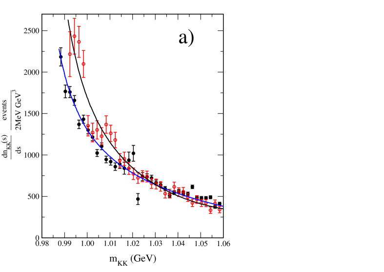
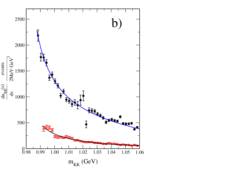
Figure 7: Comparison of $K^{+}K^{-}$ and $\overline{K}^{0}K^{+}$ $S$-wave effective mass squared distributions corrected for phase space as functions of the variable $m_{KK}$ in bins of 2 MeV [see Eqs. (92) and (96)]. The variable $m_{KK}$ is equal to $m_{K^{0}_{S}K^{+}}$ for the $\overline{K}^{0}K^{+}$ data points (open red circles) or equal to $m_{0}$ for the $K^{+}K^{-}$ data points (filled black circles). In the left panel a) the $\overline{K}^{0}K^{+}$ distribution is normalized to the number of events of the $K^{+}K^{-}$ distribution when integrated over $m_{KK}$ from the $K^{+}K^{-}$ threshold up to 1.05 GeV. In the right panel b) the $\overline{K}^{0}K^{+}$ distribution has not been renormalized. The curves correspond to the theoretical model calculations (see Sec. IV).

where $s_{0max}$ and $s_{0min}$ are the maximum and minimum $s_{0}$ values at fixed $s_{+}$. If we limit ourselves to the low $s_{+}$ values (for example, up to about 1.05 GeV²) then to a good accuracy the above distribution corresponds to the $S$-wave part of the total decay amplitude related to the isovector-scalar$a_{0}(980)^{+}$ resonance. The reason is that the dominant $P$-wave contribution, related to the $\phi(1020)$ resonance, is only present in the $K^{+}K^{-}$ decay channel. Moreover, the low-mass $K^{0}_{S}K^{+}$ and $K^{+}K^{-}$ distributions are very well separated on the Dalitz plot B10 .

For the low effective $K^{+}K^{-}$ masses one has to subtract the $P$-wave contribution. Following Ref. B5 , this can be done by calculating the spherical harmonic moments

$$\sqrt{4\pi}\langle Y^{0}_{0}(s_{0})\rangle=\int_{s_{+min}}^{s_{+max}}\frac{d^{2}N}{ds_{0}ds_{+}}ds_{+}$$ (93)

and

$$\sqrt{4\pi}\langle Y^{2}_{0}(s_{0})\rangle=\sqrt{5}\int_{s_{+min}}^{s_{+max}}P_{2}(cos\theta)\frac{d^{2}N}{ds_{0}ds_{+}}ds_{+},$$ (94)

with

$$P_{2}(cos\theta)=\frac{1}{2}(3~{}cos^{2}\theta-1),$$ (95)

and where $\theta$ is the helicity angle of the $K_{S}^{0}$ meson defined with respect to the $K^{+}$ direction in the $K^{+}K^{-}$ center-of-mass frame, $s_{+max}$ and $s_{+min}$ being the maximum and minimum $s_{+}$ values at fixed $s_{0}$. The $S$-wave $K^{+}K^{-}$ effective mass squared distribution corrected for phase space is then defined as

$$\frac{dn_{K^{+}K^{-}}(s_{0})}{ds_{0}}=\frac{\sqrt{4\pi}}{s_{+max}-s_{+min}}[\langle Y^{0}_{0}(s_{0})\rangle-\frac{\sqrt{5}}{2}\langle Y^{2}_{0}(s_{0})\rangle].$$ (96)

For completeness we give below the kinematical relation for the cosine of the helicity angle

$$cos\ \theta=\frac{s_{-}-s_{+}}{s_{+max}-s_{+min}},\hskip 28.45274pt{\rm where}\hskip 28.45274pts_{+max}-s_{+min}=4\lvert{\bf p}_{+}\rvert\lvert{\bf p}_{0}\rvert,$$ (97)

with $|{\bf p}_{+}|$ and $|{\bf p}_{0}|$ defined by Eqs. (51) and (52), respectively.

We have performed a simplified partial wave analysis of the BABAR data published in Ref. B10 . As described above, only the $S$- and $P$-waves have been included and the effective $K^{0}_{S}K^{+}$ and $K^{+}K^{-}$ masses were smaller than 1.05 GeV². The number of signal events of the $D^{0}\to\bar{K}^{0}K^{+}K^{-}$ decays was 79900$\pm$300. Based on the Dalitz plot density distributions corrected for reconstruction efficiency and background, the $S$-wave $K^{0}_{S}K^{+}$ and $K^{+}K^{-}$ effective mass distribution corrected for phase space are calculated using Eqs. (92) and (96).

The comparison of the calculated $S$-wave $K^{+}K^{-}$ and $\overline{K}^{0}K^{+}$ distributions is shown in Fig. 7. In the left panel a) a clear surplus of the $\bar{K}^{0}K^{+}$ distribution over the $K^{+}K^{-}$ one is seen below 1.02 GeV. Above $m_{KK}=1.02$ GeV the open circles corresponding to $\overline{K}^{0}K^{+}$ spectrum are in majority located below the closed circles ($K^{+}K^{-}$ events), so we observe a crossing of the two distributions. This effect is statistically significant. It was not so clear in 2005 when the first set of the BABAR data was published. But even then, in Fig. 8 of Ref. B5 , one can see the same cross-over tendency as in Fig. 7 although the statistics was lower by a factor larger than 6. In the right panel b), one sees that unrenormalized $\overline{K}^{0}K^{+}$ distribution is lower than the $K^{+}K^{-}$ distribution by a factor of about 4. The lines show the corresponding theoretical distributions based on the best fit to the Dalitz plot density distributions described in the next section.

In conclusion, the shape of the $K^{+}K^{-}$ and $\overline{K}^{0}K^{+}$ $S$-wave effective mass squared distributions, corrected for phase space, is significantly different, so in the phenomenological analysis of the $D^{0}\to\overline{K}^{0}K^{+}K^{-}$ data one cannot neglect the $f_{0}(980)$ contribution in the decay amplitude.

IV Results and discussion

The differential branching fraction or the Dalitz plot density distribution is defined as

$$\frac{d^{2}{\rm Br}}{ds_{+}ds_{0}}=\frac{|{\cal M}|^{2}}{32(2\pi)^{3}m_{D^{0}}^{3}\Gamma_{D^{0}}},$$ (98)

where ${\cal M}=\sum_{i=1}^{7}{\cal M}_{i}$ is the decay amplitude for the process studied and $\Gamma_{D^{0}}$ is the $D^{0}$ width. The decay amplitudes ${\cal M}_{i}$ have been derived in Sec. II. In Table 1 one can find some constant parameters which appear in these amplitudes.

Table 1: Values of coupling constants (in GeV) and the fixed form factors.

Parameter	Value	Reference
$f_{K^{0}}$=$f_{K^{+}}$	0.1561	JPD_PRD89
$f_{\rho}$	0.209	Beneke2003
$f_{\phi}$	0.22	Ball2007
$f_{D^{0}}$	0.2067	JPD_PRD89
$F_{0}^{D^{0}f_{0}}(m_{K^{0}}^{2})$=$F_{0}^{D^{0}a_{0}^{0}}(m_{K^{0}}^{2})$	0.18	El-Bennich_PRD79
$A_{0}^{D^{0}\rho^{0}}(m_{K^{0}}^{2})$	$0.7$	JPD_PRD89

To make a comparison of experimental data with model predictions the Dalitz diagram has been divided into five regions as shown in Fig. 8. The dimensions in different regions have been adjusted to the density of experimental events. This has been done in two steps. In the first step the units $u_{0}=8.94\times 10^{-4}$ GeV² and $u_{+}=8.97\times 10^{-4}$ GeV² corresponding to the one thousand of the full kinematic range of the variables $s_{0}$ and $s_{+}$ have been chosen. A small difference between $u_{0}$ and $u_{+}$ comes form the difference between the $K^{0}_{S}$ and $K^{+}$ masses. The cells in the ranges I, III and IV have the dimensions $11u_{0}\times 11u_{+}$ while in the range II the cells are larger having the dimensions $41u_{0}\times 41u_{+}$. Because of the high density of experimental events around the position of the $\phi(1020)$ resonance, the cells in the narrow range V have the dimensions $1u_{0}\times 35u_{+}$. In the second step we have checked whether the experimental number of events in a given cell was higher than ten. When this was not the case the adjacent cells have been combined together to group a sufficient number of events in an enlarged cell. Altogether the total number of cells was equal to $N_{cells}=1196$ (including 164 enlarged cells). The cell numbers in the regions I, II, III, IV and V were equal to 135, 282, 242, 187 and 350, respectively.

The fit of the model parameters to the experimental data has been performed using the $\chi^{2}_{tot}$ function defined as a sum of two components:

$$\chi^{2}_{tot}=\sum_{i=1}^{N_{cells}}\chi^{2}_{i}+\chi^{2}_{{\rm Br}}.$$ (99)

The value of $\chi^{2}_{i}$ for each cell $i$ has been defined as in Ref. chi2 :

$$\chi^{2}_{i}=2\Big{[}N^{exp}_{i}-N^{th}_{i}+N^{th}_{i}ln(\frac{N^{th}_{i}}{N^{exp}_{i}})\Big{]},$$ (100)

where $N^{exp}_{i}$ is a number of experimental signal events in the cell $i$ corrected for the reconstruction efficiency and $N^{th}_{i}$ is the theoretical number of events in the same cell. Including the above corrections one gets the total number of experimental events equal to $N^{exp}=80379$. The total number of theoretical events is then taken equal to $N^{exp}$.

The second component of the $\chi^{2}$ function is given by

$$\chi^{2}_{{\rm Br}}=w~{}\Big{(}\frac{{\rm Br}^{exp}-{\rm Br}^{th}}{\Delta{\rm Br}^{exp}}\Big{)}^{2}.$$ (101)

In our fit the experimental branching ratio for the decay $D^{0}\to K_{S}^{0}K^{+}K^{-}$ has been taken equal to ${\rm Br}^{exp}=4.45\times 10^{-3}$ and its error $\Delta{\rm Br}^{exp}=0.34\times 10^{-3}$. These values agree well with recent values of the Particle Data Group PDG2020 . The theoretical branching fraction ${\rm Br}^{th}$ is obtained from Eq. (98) after integrations of $\frac{d^{2}{\rm Br}}{ds_{+}ds_{0}}$ over the variables $s_{+}$ and $s_{0}$. The weight factor $w$ in our fit has been set to 100 in order to obtain a good agreement of the theoretical branching fraction with its experimental value.

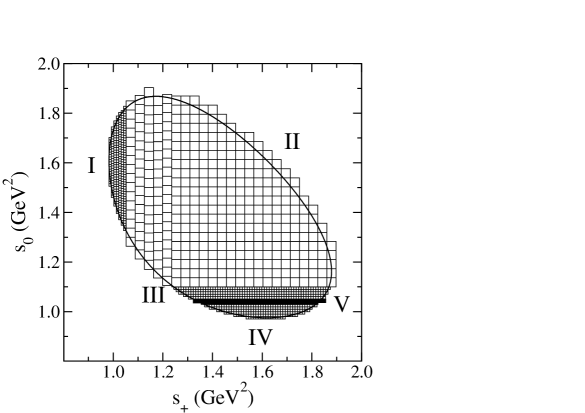
Figure 8: Partition of the Dalitz contour into five regions. Different sizes of the ($s_{+},s_{0}$) cells are shown.

We have performed many fits with our model using different parameter sets. The best fit $\chi^{2}~{}=~{}1474.4$ has been obtained with the nineteen free parameters which are displayed in Table 2. Since the number of degrees of freedom is $ndf=1196-19=1177$, the $\chi^{2}$ per degree of freedom is $\chi^{2}/ndf=1.25$.

Table 2: Parameters of our model amplitudes and their errors. Phases are given in radians.

Parameter	modulus	phase
$\chi_{n}$	22.5 GeV-1 fixed	$2.22^{+0.82}_{-0.98}$
$F_{0}^{K^{0}f_{0}}(m_{D^{0}}^{2})$	$2.22^{+0.26}_{-0.17}$	$2.21\pm 0.10$
$r_{2}$	$(5634^{+509}_{-560})$ GeV3/2
$r_{1}/r_{2}$	0.88 $\pm 0.01$
$s^{\prime}$	$(1.558^{+0.016}_{-0.014})$ GeV2
$p_{1}$	(-1.84 $\pm 0.01)$ GeV-2
$p_{2}$	(1.09 $\pm 0.01)$ GeV-4
$p_{3}$	-(0.212 $\pm 0.004)$ GeV-6
$F_{0}^{K^{-}a_{0}^{+}}(m_{D^{0}}^{2})$	$0.25^{+0.02}_{-0.03}$	$5.33^{+0.12}_{-0.08}$
$A_{0}^{K^{0}\phi}(m_{D^{0}}^{2})$	0.985 $\pm 0.007$	$3.67^{+0.12}_{-0.09}$
$M_{\phi}$	(1019.58 $\pm 0.02$) MeV
$\Gamma_{\phi}$	(4.72 $\pm 0.04$) MeV
$A_{0}^{K^{-}\rho^{+}}(m_{D^{0}}^{2})$	$9.38^{+0.63}_{-0.58}$	$5.01^{+0.06}_{-0.05}$
$P_{D}$	$5.52^{+1.25}_{-1.24}$	$3.97^{+0.23}_{-0.25}$

The value of the constant $|\chi^{n}|$ has been estimated using a relation derived similarly as Eq. (18) in Ref. AF in which the coupling constants of the $f_{0}(980)$ resonance to the $K^{+}K^{-}$ pair are taken into account instead of the $f_{0}(980)$ coupling to the $\pi\pi$ system. However, in the present case one has to include two close $f_{0}(980)$ poles sitting on the sheets (-+-) and (-++) (for their complex energy positions, $E_{R_{1}}$ and $E_{R_{2}}$, see Table 9 in Appendix A). One can generalize Eq.(18) from Ref. AF , valid for the pole position of a single resonance, to the case of two close resonances:

$$|\chi^{n}|\approx\frac{1}{|\Gamma_{2}^{n}(s_{0})|}\Big{|}\frac{g_{R_{1}K^{+}K^{-}}}{E_{R_{1}}^{2}-s_{0}}+\frac{g_{R_{2}K^{+}K^{-}}}{E_{R_{2}}^{2}-s_{0}}\Big{|},$$ (102)

where $g_{R_{1}K^{+}K^{-}}$ and $g_{R_{2}K^{+}K^{-}}$ are the coupling constants of the two $f_{0}$ resonances to $K^{+}K^{-}$. If one takes the effective $K^{+}K^{-}$ mass in the range between 960 MeV and 990 MeV then using Eq. (102) the averaged value of $|\chi^{n}|$ calculated in this range is 22.5 GeV^-1.

The magnitude of the $\chi^{s}$ parameter is taken equal to that of $|\chi^{n}|$ and its phase is set to zero. The reason for this choice is the presence of the undetermined complex value of the form factor $F_{0}^{K^{0}f_{0}}(m^{2}_{D^{0}})$ which is multiplied by $\chi^{s}$ in the ${\cal M}_{1}$ amplitude. The $F_{0}^{K^{0}f_{0}}(m^{2}_{D^{0}})$ value results from the fit to data.

The form factors $\Gamma_{2}^{n}(s_{0})$ and $\Gamma_{2}^{s}(s_{0})$ have been calculated in a three-channel model of meson-meson interactions ($\pi\pi$, $K\bar{K}$ and an effective $2\pi\ 2\pi$), introduced in Ref. DedonderPol . These form factors depend not only on the values of the meson-meson parameters listed in Table 8 in Appendix A but also on two other parameters $\kappa$ and $c$ defined by Eqs. (28) and (39) in Ref. DedonderPol , respectively. Their values $\kappa=2807.3$ MeV and $c=0.109$ GeV^-4 have been fitted to the $B^{\pm}\to K^{\pm}K^{+}K^{-}$ decay data analyzed in Ref. KKK .

In Fig. 9 we show the effective energy dependence $E$ of moduli and phases of the $K\overline{K}$ isoscalar-scalar nonstrange $\Gamma_{2}^{n}(E)$ and strange $\Gamma_{2}^{s}(E)$ form factors. The energy $E$ is equal to the square root of $s$.

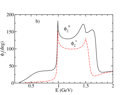
Figure 9: a) moduli of the isoscalar-scalar kaon nonstrange $\Gamma_{2}^{n}(E)$ (solid line) and strange $\Gamma_{2}^{s}(E)$ (dashed line) form factors; b) the corresponding phases.

In the above model the kaon threshold energy was set equal to the sum of the charged and neutral kaon masses. However, the ${\cal M}_{1}$ amplitude corresponds to the isoscalar $K^{+}K^{-}$ $S$-wave state with a threshold lower by about 3.9 MeV in comparison with the $K^{+}K^{0}_{S}$ threshold energy. In order to take this effect into account in an approximate way, we introduce the variable

$$\bar{s}_{0}=s_{0}\ \frac{s_{av}}{s_{th}}$$

with $s_{th}=4m_{K}^{2}$ and the correction factor is $s_{av}/s_{th}=1.008172$. The kaon form factors have to be evaluated at this argument, i.e., $\Gamma_{2}^{n}(\bar{s}_{0})$ and $\Gamma_{2}^{s}(\bar{s}_{0})$. To improve the quality of the data fit the form factors $\Gamma_{2}^{n}(\bar{s}_{0})$ and $\Gamma_{2}^{s}(\bar{s}_{0})$ have been multiplied by the function

$$P(s_{0})=\frac{1-\frac{s_{0}-s_{th}}{s^{\prime}-s_{th}}}{1+bs_{0}^{3}},$$ (103)

where $s^{\prime}$ is a new parameter which is fitted to the data (see Table 2). It corresponds to a zero of $P(s_{0})$. The third order polynomial in the denominator, with the constant $b$ fixed to 0.0154 GeV^-6, is introduced in order to control asymptotically the high energy behavior of the ${\cal M}_{1}$ amplitude. This denominator replaces the denominator $(1+cE^{4})$ with $E=\sqrt{s_{0}}$ in Eq. (39) of  DedonderPol . A plot of the function (103) used in our fit is shown as the continuous black line denoted R_BF in Fig. 16 (a) where it is compared to the corresponding functions used in the two alternative fits MO_P1(P2) described in Appendix B. This function reduces the moduli of the amplitudes which depend on the isoscalar-scalar form factors.

The masses and widths of the isovector-scalar resonances $a_{0}(980)$ and $a_{0}(1450)$ are presented in Table LABEL:Table_a0. They have been fixed during the minimization of the $\chi^{2}$ function. The parameters of the $a_{0}(1450)$ on sheet $(-~{}-)$ were taken from Ref. PDG2020 . However, we have studied the influence of the position of the $a_{0}(980)$ pole on sheet $(-~{}+)$ in the complex energy domain on the $\chi^{2}$ minimum curve. In this way the $a_{0}(980)$ mass and width on sheet $(-~{}+)$ have been determined together with an estimation of their errors. The masses and widths of other two associated $a_{0}$ poles are also given in Table LABEL:Table_a0.

Table 3: Parameters of resonances $a_{0}(980)$ and $a_{0}(1450)$.

	mass (MeV)	width (MeV)	Riemann sheet
$a_{0}(980)$	$979^{+3}_{-2}$	$25^{+8}_{-6}$	$-~{}~{}+$
$a_{0}(980)$	$959$	$34$	$-~{}~{}-$
$a_{0}(1450)$	$1474$	$132$	$-~{}~{}-$
$a_{0}(1450)$	$1470$	$91$	$-~{}~{}+$

Table 4: Potential parameters of the $K\overline{K}$ $S$-wave isospin one interaction.

$\beta_{1}$	21.662 GeV
$\beta_{2}$	21.831 GeV
$\lambda_{1}$	$-2.9850\times 10^{-2}$
$\lambda_{2}$	$-6.7977\times 10^{-2}$
$\lambda_{12}^{2}$	$2.2142\times 10^{-7}$

The coupled channel model of the $a_{0}(980)$ and $a_{0}(1450)$ resonances described in Ref. AFLL has been implemented. There, the separable $\pi\eta$ and $K\overline{K}$ interactions have been used in the calculation of the $S$-wave isospin one scattering amplitudes. Altogether the model has five parameters: two range parameters $\beta_{1}$ and $\beta_{2}$, two channel coupling constants $\lambda_{1}$ and $\lambda_{2}$, and the interchannel coupling constant $\lambda_{12}$ (here the channel $\pi\eta$ is labeled by $1$ and the channel $K\overline{K}$ by $2$). The potential parameters are given in Table LABEL:pot_param. There exist direct numerical relations between the four parameters describing the positions of the $a_{0}(980)$ and $a_{0}(1450)$ resonances in the complex energy plane (Table LABEL:Table_a0) and the four potential parameters $\beta_{1}$, $\lambda_{1}$, $\lambda_{2}$ and $\lambda_{12}$ at fixed value of the fifth parameter $\beta_{2}$. These relations are given in Ref. LL .

The function $G_{1}(s)$ is introduced to describe a transition from the $u\bar{u}$ pair to the $K\overline{K}$ spin zero isospin one state. Two isovector-scalar resonances $a_{0}(980)$ and $a_{0}(1450)$ can be formed during that transition. Both resonances are also coupled to the $\pi\eta$ state. Therefore it is natural to consider three cases for the transition from the $u\bar{u}$ pair to the $K\overline{K}$ state. In the first case the $K\overline{K}$ pair is directly formed from the $u\bar{u}$ pair. In the second case the $K\overline{K}$ pair undergoes the elastic rescattering in the final state. In the third case the intermediate $\pi\eta$ pair is formed and then the inelastic transition to the $K\overline{K}$ state takes place. The interaction between the meson-meson pairs is treated in the framework of the separable potential model fully described in Ref. LL and used to study the properties of the $a_{0}$ resonances (Refs. AFLL , AFLL2 ).

Below we briefly derive the dependence of the $G_{1}(s)$ function on the meson-meson transition amplitudes. Labelling by 1 the $\pi\eta$ channel and by 2 the $K\overline{K}$ channel, one can express $G_{1}(s)$ as a superposition of three terms:

$$G_{1}(s)=R_{2}(s)+I_{22}(s)+I_{12}(s),$$ (104)

where

$$R_{2}(s) = r_{2}\ W(s)\ g_{2}(k_{2}),$$ (105)

$$I_{22}(s) = r_{2}\ W(s)\ \frac{T_{22}(s)}{g_{2}(k_{2})}\ C_{2}(s),$$ (106)

$$I_{12}(s) = r_{1}\ W(s)\ \frac{T_{12}(s)}{g_{1}(k_{1})}\ C_{1}(s).$$ (107)

Here $r_{1}$ and $r_{2}$ are the coupling constants corresponding to the $u\bar{u}$ transitions to the $\pi\eta$ and $K\overline{K}$ states, respectively. The function $W(s)$ is the third-degree polynomial

$$W(s)=1+p_{1}s+p_{2}s^{2}+p_{3}s^{3}.$$ (108)

where $p_{1}$, $p_{2}$ and $p_{3}$ are the real parameters included in the list of the model free parameters (see Table 2). We keep the same $p_{j},j=1,2,3$, parameters for both channels. The fitted polynomial $W(s_{0})$ is plotted as the continuous black line in Fig. 16(b) where it is compared to the polynomial $P_{F}(s_{0})$ defined by Eq. (113) and used in the alternative MO_P1(P2) fits discussed in Appendix B. The introduction of these polynomials improves the quality of the $\chi^{2}$ fit, in particular in the region II where the density of events is small. The functions $g_{i}(k_{i}),i=1,2$, are the vertex functions

$$g_{i}(k_{i})=\sqrt{\frac{2\pi}{m_{i}}}\frac{1}{k_{i}^{2}+\beta_{i}^{2}},$$ (109)

where $m_{i}$ are the channel reduced masses, $k_{i}$ are the channel momenta and $\beta_{i}$ are the range parameters. In the $\pi\eta$ channel $m_{1}=m_{\pi}m_{\eta}/(m_{\pi}+m_{\eta})$, in the $K\overline{K}$ channel $m_{2}=m_{K}/2$. We take the neutral $\pi$ mass $m_{\pi}=134.977$ MeV and $m_{\eta}=547.862$ MeV. The function $T_{22}(s)$ in Eq. (106) is the elastic $K\overline{K}$scattering amplitude and $T_{12}(s)$ in Eq. (107) denotes the transition amplitude from the $\pi\eta$ channel to the $K\overline{K}$ channel. In Eq. (106) one finds the integral

$$C_{2}(s)=\int\frac{d^{3}p}{(2\pi)^{3}}\frac{g_{2}^{2}(p)}{E+i\epsilon-2E_{K}(p)}$$ (110)

and in Eq. (107) we have

$$C_{1}(s)=\int\frac{d^{3}p}{(2\pi)^{3}}\frac{g_{1}^{2}(p)}{E+i\epsilon-E_{\pi}(p)-E_{\eta}(p)},$$ (111)

where the energies are defined as $E=\sqrt{s}$, $E_{K}(p)=\sqrt{p^{2}+m_{K}^{2}}$, $E_{\pi}(p)=\sqrt{p^{2}+m_{\pi}^{2}}$ and $E_{\eta}(p)=\sqrt{p^{2}+m_{\eta}^{2}}$. The modulus and the phase of the resulting $G_{1}(s)$ function are plotted in Figs. 10 (a) and 10 (b), respectively.

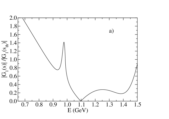
Figure 10: a) modulus of the $G_{1}(s)$ function normalized to 1 at the $K^{+}K^{-}$ threshold; b) phase of the $G_{1}(s)$ function ($E={\sqrt{s}}$). At threshold $G_{1}(s_{th})$ = 304.69 GeV^-1.

The importance of the annihilation diagrams in the description of the experimental data should be here underlined. The annihilation terms, proportional to $f_{D^{0}}$, are present in all the decay amplitudes ${\cal M}_{i}$ and their magnitudes strongly dominate over other amplitudes which contribute to the total decay amplitude. The annihilation amplitudes depend on the appropriate form factors calculated for the momentum transfer squared $m_{D^{0}}^{2}$. These fitted form factors are given in the second, ninth, tenth and thirteenth rows of Table 2.

The mass and the width of the $\phi(1020)$ resonance seen in Table 2 are in agreement with the corresponding BABAR values of ($1019.55\pm 0.02$) MeV and ($4.60\pm 0.04$) MeV, respectively B10 . The obtained width is higher, by about 0.5 MeV, than the averaged value of ($4.249\pm 0.013$) MeV given by the Particle Data Group in Ref. PDG2020 . This can be explained by a finite experimental energy resolution.

The branching fraction distributions $\frac{d^{2}{\rm Br}_{i}}{ds_{+}ds_{0}}$ corresponding to the amplitudes ${\cal M}_{i}$, $i=1,...,7$ are obtained if in Eq. (98) the amplitude ${\cal M}$ is replaced by ${\cal M}_{i}$. One can also define the off-diagonal elements $\frac{d^{2}{\rm Br}_{ij}}{ds_{+}ds_{0}}$, $i\neq j$,

$$\frac{d^{2}{\rm Br}_{ij}}{ds_{+}ds_{0}}=\frac{Re[{\cal M}_{i}^{*}{\cal M}_{j}]}{32(2\pi)^{3}m_{D^{0}}^{3}\Gamma_{D^{0}}}.$$ (112)

If we integrate over $s_{+}$ and $s_{0}$ the differential branching fractions $\frac{d^{2}{\rm Br}}{ds_{+}ds_{0}}$, $\frac{d^{2}{\rm Br}_{i}}{ds_{+}ds_{0}}$ and $\frac{d^{2}{\rm Br}_{ij}}{ds_{+}ds_{0}}$ then we get the corresponding branching fractions ${\rm Br}$, ${\rm Br}_{i}$, $i=1$ to 7 or the off-diagonal elements ${\rm Br}_{ij}$, where $i\neq j$. The matrix ${\rm Br}_{ij}$ is symmetric: ${\rm Br}_{ij}={\rm Br}_{ji}$.

Table 5: Branching fractions (Br) for different quasi-two-body channels in the best fit to the BABAR data B10 .

Amplitude	channel	Bri ($\%$)
${\cal{M}}_{1}$	$[K^{+}\,K^{-}]_{S}\,K^{0}_{S}$	$60.9^{+24.4}_{-10.6}$
${\cal{M}}_{2}$	$[K^{+}\,K^{-}]_{P}\,K^{0}_{S}$	$45.5\pm{0.7}$
${\cal{M}}_{3}$	$[K^{0}_{S}\,K^{+}]_{S}\,K^{-}$	$20.7^{+9.4}_{-6.0}$
${\cal{M}}_{4}$	$[K^{0}_{S}\,K^{+}]_{P}\,K^{-}$	$21.5^{+3.1}_{-2.8}$
${\cal{M}}_{5}$	$[K^{0}_{S}\,K^{-}]_{S}\,K^{+}$	$0.76^{+0.18}_{-0.15}$
${\cal{M}}_{6}$	$[K^{0}_{S}\,K^{-}]_{P}\,K^{+}$	$0.08\pm 0.01$
${\cal{M}}_{7}$	$[K^{+}\,K^{-}]_{D}\,K^{0}_{S}$	$0.05\pm 0.02$
$\sum_{i=1,7}$ Bri		$149.5^{+26.9}_{-12.3}$

In Table 5 we give uncertainties of the branching fractions. They have been obtained by choosing 10 000 different combinations of the 19 model parameters. The parameters values have been generated from the Gaussian distributions taking into account the parameter uncertainties written in Table 2 and some correlations between the parameters in the amplitudes ${\cal{M}}_{1}$ and ${\cal{M}}_{3}$. Then the branching fraction uncertainties have been obtained from the distributions of the 10 000 values of each branching fraction and of their sum.

Let us notice the particularly large uncertainties of the branching fraction ${\rm Br}_{1}=60.9^{+24.4}_{-10.6}\%$. This is due to the fact that the amplitude ${\cal{M}}_{1}$ consists of three components and contains 9 free parameters.

As seen in Table 5 the largest contribution (near 61 $\%$) to the summed branching fraction ${\rm Br}~{}=~{}\sum_{i=1}^{7}{\rm Br}_{i}$ comes from the first amplitude ${\cal M}_{1}$. It corresponds to the quasi-two body channel consisting of $K^{0}_{S}$ and the $K^{+}K^{-}$ pair in the $S$-wave. The second contribution (near 46 $\%$) to the integrated branching fraction ${\rm Br}$ is due to the amplitude ${\cal M}_{2}$. In this case the $K^{+}K^{-}$ pair is in the $P$-wave and its major part is related to the $\phi(1020)$ resonance. This resonance largely dominates in the region V of the Dalitz diagram.

There are two almost equal contributions of about 21$\%$ from the channels $[K^{0}_{S}\,K^{+}]_{S}\,K^{-}$ and $[K^{0}_{S}\,K^{+}]_{P}\,K^{-}$ (amplitudes ${\cal M}_{3}$ and ${\cal M}_{4}$, respectively). The ${\cal M}_{3}$ amplitude can be related to a presence of the two isovector-scalar resonances $a_{0}(980)$ and $a_{0}(1450)$. As seen in Table LABEL:Table_a0 the mass of the resonance $a_{0}(980)$ equal to $979^{+3}_{-2}$ on sheet $-+$ is lower than the $K^{0}_{S}K^{+}$ threshold mass of about 991.3 MeV. However, due its finite width of $25^{+8}_{-6}$ MeV, this resonance, together with the second $a_{0}(980)$ resonance on sheet $--$ at ($959-i~{}34$) MeV, can strongly influence the near threshold $s_{+}$ range of the Dalitz plot density distribution. On the other hand, the mass of the $a_{0}(1450)$ resonance lies above the upper range of the $K^{0}_{S}K^{+}$ effective mass close to 1371 MeV. However, the $a_{0}(1450)$ resonances are wide and they can also affect the distribution of the $D^{0}\to K^{+}K^{-}K^{0}_{S}$ events on the Dalitz plot.

The contribution of the quasi-two body channel $[K^{0}_{S}\,K^{+}]_{P}\,K^{-}$ is related to nonzero couplings of the $P$-wave resonances $\rho(770)^{+}$, $\rho(1450)^{+}$ and $\rho(1700)^{+}$ to $K^{0}_{S}K^{+}$. Although the $\rho(770)^{+}$ mass lies below the $K^{0}_{S}\,K^{+}$ threshold its width is sufficiently large to influence the differential density distribution of the Dalitz plot for $s_{+}$ values above the threshold. The $\rho(1450)^{+}$ width is even larger than that of $\rho(770)^{+}$, so the whole $s_{+}$ range on the Dalitz plot is sensitive to the strength of its coupling to $K^{0}_{S}\,K^{+}$. The above three $\rho$ resonances, being wide, cannot create a clear structure or a well distinguished band on the Dalitz plot. This could be a reason why they have not been included in the isobar model analyses B10 and  B5 .

These results can be compared to the results of the experimental analysis which finds a summed branching fraction of 163.4 %, mainly with 71.1 % coming from the $a_{0}(980)^{0}$ and $a_{0}(1450)^{0}$, 44.1 % from the $\phi(1020)$ resonance and 45.1 % from the $a_{0}(980)^{+}$ and $a_{0}(1450)^{+}$.

Table 6: Matrix of the branching fractions components Br_ij (Eq. (112)) for the best fit to the BABAR data B10 . All numbers are in per cent.

	${\cal{M}}_{1}$	${\cal{M}}_{2}$	${\cal{M}}_{3}$	${\cal{M}}_{4}$	${\cal{M}}_{5}$	${\cal{M}}_{6}$	${\cal{M}}_{7}$
${\cal{M}}_{1}$	60.92	0.00	2.99	-20.76	-2.49	-0.69	0.00
${\cal{M}}_{2}$		45.52	-3.37	-1.29	-0.66	-0.06	0.00
${\cal{M}}_{3}$			20.73	0.00	-0.21	0.52	0.13
${\cal{M}}_{4}$				21.47	0.61	0.58	-0.06
${\cal{M}}_{5}$					0.76	0.00	0.01
${\cal{M}}_{6}$						0.08	0.00
${\cal{M}}_{7}$							0.05

In Table 6 the diagonal branching fraction terms already shown in Table 5 are given together with the off-diagonal terms ${\rm Br}_{ij}$. The sum of the off-diagonal terms equals to -$49.53~{}\%$. One should remark here that some off-diagonal terms are exactly equal to zero. This is due to the orthogonality of certain wave functions. For example, the interference term ${\rm Br}_{12}$ vanishes since the wave functions of the $S$- and $P$-states of the $K^{+}K^{-}$ system are orthogonal. Due to the matrix symmetry the elements of the branching fractions below the diagonal are not written.

The amplitude ${\cal M}_{1}$ is a sum of three terms [see Eqs. (79)-(82)]. The first isoscalar term is proportional to the conjugated kaon nonstrange scalar form factor $\Gamma_{2}^{*n}(s_{0})$ and the second one to the conjugated kaon strange scalar form factor $\Gamma_{2}^{*s}(s_{0})$. The third term is proportional to the function $G_{1}(s_{0})$ describing the transition from the $u\bar{u}$ pair of quarks into the $K^{+}K^{-}$ pair of mesons in the isospin one and spin zero state.

Table 7: Matrix of the branching fraction components Br of the ${\cal{M}}_{1}$ amplitude calculated for the best fit to the BABAR data B10 . All numbers are in per cent.

	${\cal{M}}^{n,I=0}_{1}$	${\cal{M}}^{s,I=0}_{1}$	${\cal{M}}^{I=1}_{1}$
${\cal{M}}^{n,I=0}_{1}$	1.19	-7.32	-0.36
${\cal{M}}^{s,I=0}_{1}$		59.82	5.40
${\cal{M}}^{I=1}_{1}$			4.48

In Table LABEL:TabBr123 the diagonal and the off-diagonal components of the branching fraction related to the ${\cal M}_{1}$ amplitude are given. They are defined in a similar way as the ${\rm Br}_{ij}$ components in Eq. (112). From this Table we see that the major contribution close to 60% is related to the strange scalar isospin zero component of the annihilation ($W$-exchange) amplitude ${\cal M}_{1}^{s,I=0}$. Here the isoscalar-scalar resonances like $f_{0}(980)$ are formed from the strange-antistrange pair of quarks. Following the result of the fit shown in the above Table the formation of the isoscalar-scalar resonances from the $u\bar{u}$ quarks is suppressed (the diagonal ${\cal M}_{1}^{n,I=0}$ branching fraction is equal only to 1.19 %). Also the branching fraction equal to 4.48%, corresponding to the isovector-scalar amplitude ${\cal M}_{1}^{I=1}$, is much smaller than that related to the ${\cal M}_{1}^{s,I=0}$ amplitude. The sum of all the off-diagonal components equals to -4.57 %. A comparison of the results for this best fit model with those for the alternative MO_P1(P2) ones can be found in the Appendix B.

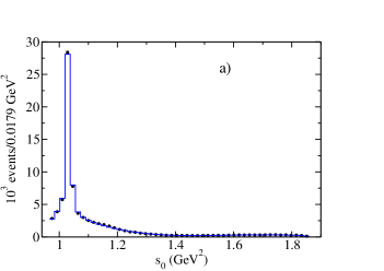
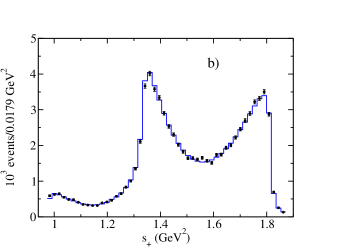
Figure 11: Dalitz plot projections for $D^{0}~{}\to K^{0}_{S}K^{+}K^{-}$. The points indicate the BABAR data B10 together with their statistical errors. Histograms represent the best fit theoretical distributions.

Dalitz plot projections or one-dimensional effective mass squared distributions of events are calculated by a proper integration of the two-dimensional density distributions. They are shown in Fig. 11. The errors of the experimental signal weighted event number distributions are the statistical ones. The histograms correspond to the theoretical distributions normalized to the same total number of events.

The distribution in Fig. 11(a) is strongly dominated by the maximum corresponding to the $\phi(1020)$ resonance decaying to the $K^{+}K^{-}$ pair. This decay is in the $P$-wave and leads to a characteristic two-maximum shape of the Dalitz plot distribution as a function of $s_{+}$ - the square of the $K^{+}K^{-}$ effective mass. Since the branching fraction for the channel $[K^{+}\,K^{-}]_{P}\,K^{0}_{S}$ is large (45.5 %) the two Dalitz projections in Figs. 11(b) and(c) have a two-maximum character. There are also two other important contributions related to the amplitudes ${\cal M}_{1}$ and ${\cal M}_{3}$. However, they do not produce any pronounced structures on the Dalitz plot since both are due to the $S$-wave in the $K^{+}K^{-}$ or in the $K^{0}_{S}\,K^{+}$ configuration.

Finally let us discuss the low effective mass parts of the $K^{+}K^{-}$ and $K^{0}_{S}\,K^{+}$ distributions ($m_{KK}<1.06$ GeV). Since the differential branching fraction [Eq. (98)] is proportional to the Dalitz plot density distribution of events $\frac{d^{2}N}{ds_{+}ds_{0}}$, one can calculate the theoretical one-dimensional distributions of the event numbers using Eqs. (92)-(94) of Sec. III. They are displayed in Fig. 11 as solid histograms. One can see that the BABAR data agree well with the corresponding lines. This agreement enforces the statement about the significant difference between the $K^{+}K^{-}$ and $K^{0}_{S}\,K^{+}$ effective mass distributions which is due to the dominant $f_{0}(980)$ resonance contribution to the $K\bar{K}$ final state interaction amplitude.

V CONCLUSIONS

A theoretical model of the $D^{0}\to K_{S}^{0}K^{+}K^{-}$ decay amplitude has been constructed within a quasi-two-body QCD factorization approach introducing scalar kaon form factors to describe the $S$-wave kaon-kaon final  state interaction. In doing so, the contribution of isoscalar-scalar $f_{0}$ resonance family, viz. $f_{0}(980),f_{0}(1370)$ and  that of the isovector-scalar $a_{0}$ one, viz. $a_{0}^{0}(980),a_{0}^{\pm}(980),a_{0}^{0}(1450),a_{0}^{\pm}(1450)$ are taken into account. The isospin zero and one kaon-kaon $S$-wave interactions have been treated in a unitary way using either coupled channel relativistic equations, or a dispersion relation framework. The $P$- and $D$- waves of the final state kaon-kaon interactions have also been taken into account.

Independently of any model assumptions, we have shown that the $K^{+}K^{-}$ and $\bar{K}^{0}K^{+}$ $S$-wave effective mass squared distributions, corrected for phase space, are significantly different. This means that, in the analyses of the $D^{0}\to\bar{K}^{0}K^{+}K^{-}$ data, one cannot neglect the contribution of the $f_{0}(980)$ resonance and retain only the $a_{0}(980)$ contribution.

In Appendix A, we have updated the meson-meson $S$-wave isospin zero scattering amplitudes. These include the three coupled, $\pi\pi$, $\bar{K}K$ and an effective $2\pi\ 2\pi$ channels. Using the above amplitudes the new kaon nonstrange and strange form factors $\Gamma_{2}^{n}(s_{0})$ and $\Gamma_{2}^{s}(s_{0})$ have been calculated following Ref. KKK and introduced in the data analysis. As seen Fig. 14, these form factors are quite similar to those derived using the Muskhelishvili-Omnès dispersion relation approach Moussallam_2000 ; Moussallam_2019 .

In the factorization framework, for the $D^{0}\to K^{0}_{S}K^{+}K^{-}$ process one has to evaluate the matrix elements of the $D^{0}$ transitions to two-kaons or the transitions between one kaon and two kaons. The knowledge of these transitions requires that of the three-body strong interaction between the $D^{0},K^{0}_{S}$ and $K^{\pm}$ mesons and that between the $K^{0}_{S},K^{+}$ and $K^{-}$ mesons. Here, to describe these transitions with the two final kaons in $S$-wave state, we had to go beyond the simple multiplication of the scalar kaon form factors by a complex constant. And to obtain good fits we have multiplied the isoscalar-scalar kaon form factor by a one free parameter energy-dependent function and introduced into the isovector-scalar function an energy-dependent phenomenological polynomial involving three free parameters.

The undetermined free parameters of our seven $D^{0}\to K^{0}_{S}K^{+}K^{-}$ amplitudes are then related to the strength of the isoscalar-scalar kaon form factor, to the function proportional to the isovector-scalar kaon form factor and to the unknown meson to meson transition form factors. They are obtained through a $\chi^{2}$ minimization to the BABAR Dalitz plot distribution B10 . It should be pointed out that the low density of events in the central region of this Dalitz plot distributions (see Fig. 8) is difficult to reproduce. Using unitary relativistic equations to built the isoscalar-scalar form factor and a function proportional to the isovector-scalar one, we obtain a best fit (denoted R_BF), with a $\chi^{2}/ndf$ of 1.25 with 19 free parameters to be compared to that of 1.28 for Ref. B10 which uses 17 free parameters.

In Appendix B, we have studied two alternative fits with scalar-kaon form factors derived in the Muskhelishvili-Omnès dispersion relation framework. All other amplitudes are parametrized as in the best fit model. If the scalar form factors are multiplied by energy dependent phenomenological functions, we obtain two good fits, one, denoted MO_P1 with a $\chi^{2}/ndf$ of 1.32 and 16 free parameters and another one, MO_P2, with a $\chi^{2}/ndf$ of 1.31 and 16 free parameters.

Our fits indicate the dominance of the annihilation amplitudes and for the best fit a large dominance of the $[K^{+}K^{-}]_{S}$ isospin 0 $S$-wave contribution and a sizable branching fraction to the $[K^{0}_{S}K^{+}]_{P}K^{-}$ final state with the $[K^{0}_{S}K^{+}]$ pair coupled to $\rho(770)^{+}$, $\rho(1450)^{+}$ and $\rho(1700)^{+}$. The alternative fits show important contributions from both the $f_{0}$ and $a_{0}^{0}$ mesons and a weaker $\rho^{+}$ mesons role. For all our models, the one-dimensional distributions agree well with that of the BABAR data.

One can estimate the strength of the contributions of the different amplitudes by looking at their branching ratio compared to the sum of their branching ratios. As can be seen in Table LABEL:TabBr45Req for the best fit model this sum is 149.5 [126.3, 164.1] % (163.4% in Ref. B10 ), which points to sizable interference contributions. The kaon-kaon S-wave interactions, related to the $f_{0}$ and $a_{0}^{0}$ resonances, gives a large branching of $\sim$61 [45, 63] % with a large value (for BF, MO_P1 and MO_P2, see Table LABEL:TabBr45Reqa) of $\sim$60 [23, 46] %, for the amplitude proportional to the strange isoscalar-scalar form factor ($f_{0}$ contributions) and smaller branching $\sim$5 [16,16] % for the amplitude proportional to the isovector-scalar form factor ($a_{0}^{0}$ contributions). Corresponding figures in the isobar BABAR analysis B10 are $\sim$71 %, dominated by the $a_{0}(980)^{0}$ and $a_{0}(1450)^{0}$ with no $f_{0}(980)$ and a $f_{0}(1370)$ $\sim$ 2% .

The branching fraction of the isospin 0 $P$-wave $\sim$46 [45, 45] %, dominated by the $\phi(1020)$ resonance, is similar to that found, $\sim$44 %, in Ref. B10 . The branching of the isovector amplitude associated to the $a_{0}^{+}$ resonances is $\sim$21 [26, 40] % to be compared to $\sim$ 45 % in Ref. B10 . The branching fraction of the amplitude related to the $[\rho(770)^{+}+\rho(1450)^{+}+\rho(1700)^{+}]K_{S}^{0}$ final state, not introduced in Ref. B10 , has a value of $\sim$22 [8, 13] %. One could say that, this contribution with no bumps in the Dalitz plot distribution, is in Ref.B10 taken into account by a part of that of the $a_{0}^{+}$.

The charmless hadronic $B^{0}\to K^{+}K^{-}K_{S}^{0}$ studied by the Belle Be2010 and BABAR BA2012 Collaborations has the same meson final states as the $D^{0}$ decay we have been studied here. A quasi-two-body QCD factorization analysis of this $B^{0}$ decay process should allow, to constrain, not only the weak interaction observables but also the scalar kaon form factors, the transitions between one kaon and two kaons and to learn about the $B^{0}$ transition to two kaons.

Appendix A Updated $\pi\pi$, $\bar{K}K$ and effective $2\pi\ 2\pi$ $S$-wave amplitudes

Here we present updated results for the meson-meson $S$-wave isospin zero scattering amplitudes. They include the following three coupled channels: $\pi\pi$, channel 1, $\bar{K}K$, channel 2 and effective $2\pi\ 2\pi$, channel 3. Our previous fits to the meson-meson scattering data were obtained in the late nineties KLL ; EPJ . Since, new precise low energy $\pi\pi$ data have appeared NA48 . Moreover, as noticed by Bachir Moussallam Moussallam_Nov2018 , we used an assumption valid only below the opening of the third channel, namely the phase of the $\pi\pi~{}\to~{}\bar{K}K$ transition amplitude was set equal to the sum of the elastic $\pi\pi$ and $\bar{K}K$ phaseshifts. The derivation of the kaon isoscalar-scalar form factors $\Gamma_{2}^{n}(s_{0})$ and $\Gamma_{2}^{s}(s_{0})$, used in the present analysis for $s_{0min}=0.98$ GeV${}^{2}~{}\leq~{}s_{0}~{}\leq~{}s_{0max}=1.87$ GeV², requires the knowledge of the meson-meson amplitudes at energies above $s_{0max}$.

Thus, dropping the above mentioned assumption, we have performed a new analysis based on an enlarged set of data. Using the same three coupled-channel separable potential model as developed in Refs. KLL and EPJ , we fit the following data:

a) for the effective $\pi\pi$ mass $E$ between 286 and 390 MeV, the 10 values of the elastic $\pi\pi$ phase shifts from the NA48 data NA48 ,

b) for $610$ MeV$\leq~{}E~{}\leq 1580$ MeV, the 50 values of the $\pi\pi$ phase shifts $\delta_{\pi\pi}$ and for $1010$ MeV$\leq~{}E~{}\leq 1580$ MeV the 30 values of the $\pi\pi$ inelasticities $\eta_{\pi\pi}$, both quantities obtained in the experimental analysis of Ref. KLRyb ,

c) for $995$ MeV$\leq~{}E~{}\leq 1580$ MeV, the 23 values of the moduli of the transition $\pi\pi\to\overline{K}K$ amplitude $T_{12}$ extracted from Fig. 27 of Ref. Cohen ,

d) for the $\delta_{\pi\pi\to K\overline{K}}$ phases of the $T_{12}$ amplitude, the 21 values extracted in the analysis of Ref. Cohen for $1016$ MeV$\leq~{}E~{}\leq 1530$ MeV,

e) plus the 6 data points for these phases between 1538 and 1741 MeV determined in Ref. Etkin .

The total number of fitted data is then equal to 140. As in Ref. KLL , the fitting method is based on the $\chi^{2}$ function being a sum of five components related to the five data sets enumerated above. The resulting $\chi^{2}$ is equal to 135.04 which, for 14 free model parameters, gives the value $\chi^{2}/ndf=1.07$ when divided by $ndf=140-14=126$ degrees of freedom.

Table 8: Model parameters fitted to data.

Parameter	value
$\Lambda_{11,1}$	-0.14434 $\cdot 10^{-3}$
$\Lambda_{11,2}$	-0.21102
$\Lambda_{22}$	-0.62730
$\Lambda_{33}$	-0.81318$\cdot 10^{-3}$
$\Lambda_{12,1}$	0.25184$\cdot 10^{-4}$
$\Lambda_{12,2}$	0.033294
$\Lambda_{13,1}$	0.25063$\cdot 10^{-4}$
$\Lambda_{13,2}$	-0.34913
$\Lambda_{23}$	-5.4206
$\beta_{1,1}$	3.0366$\cdot 10^{3}$  GeV
$\beta_{1,2}$	1.1019  GeV
$\beta_{2}$	0.98412  GeV
$\beta_{3}$	0.047940  GeV
$m_{3}$	0.75200  GeV

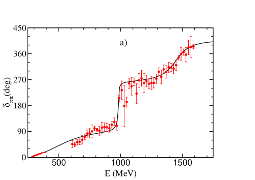
Figure 12: Comparison to the data of our fit (solid line): a) the $\pi\pi$ elastic phase shifts versus the $\pi\pi$ center-of-mass energy $E$, b) the $\pi\pi$ inelasticities and for energies $E$ higher than the $\overline{K}K$ mass threshold. The data below $E$ = 400 MeV are taken from Ref. NA48 and those above 600 MeV from Ref. KLRyb for the “down-flat” solution.

Table 9: Positions of $S$ matrix poles ($E$ in MeV).

		Sign of
Re $E$	Im $E$	Im $k_{1}$ Im $k_{2}$ Im $k_{3}$	n∘
227	0	$-$     $-$     $-$	I
230	0	$-$     $-$     $+$	II
230	0	$+$     $-$     $-$	III
232	0	$+$     $-$     $+$	IV
485	-233	$-$     $+$     $-$	V
485	-233	$-$     $+$     $+$	VI
506	-262	$-$     $-$     $-$	VII
507	-265	$-$     $-$     $+$	VIII
967	-10	$-$     $+$     $-$	IX
982	-8	$-$     $+$     $+$	X
1442	-100	$-$     $+$     $-$	XI
1444	-93	$-$     $+$     $+$	XII
1448	-97	$-$     $-$     $+$	XIII
1465	-98	$-$     $-$     $-$	XIV
1553	-211	$+$     $-$     $-$	XV
1559	-213	$-$     $-$     $-$	XVI
1581	-138	$-$     $-$     $+$	XVII
1584	-134	$+$     $-$     $+$	XVIII

Table 10: Coupling constants $g_{i}$ in GeV for a few representative $S$-matrix poles ($E$ in MeV).

Re $E$	Im $E$	$|g_{1}|^{2}/4\pi$	$|g_{2}|^{2}/4\pi$	$|g_{3}|^{2}/4\pi|$	n∘
506	-262	0.86	0.03	0.00	VII
967	-10	0.08	1.68	0.05	IX
982	-8	0.07	1.27	0.04	X
1448	-97	1.02	0.08	0.16	XIII
1559	-213	0.07	2.24	0.77	XVI

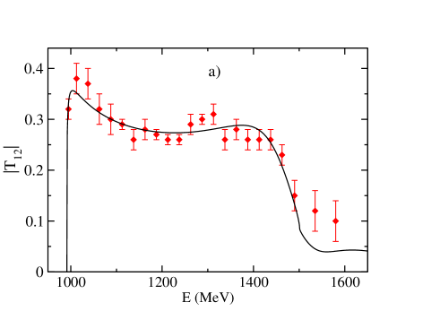
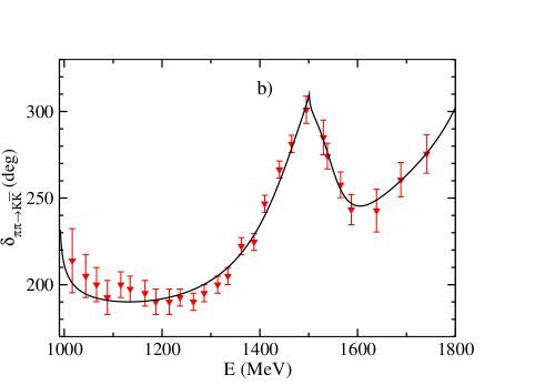
Figure 13: Comparison to the data Cohen of our fit (solid line): a) Modulus of the $\pi\pi\to\bar{K}K$ transition amplitude $T_{12}(E)$ normalized as in Ref. Cohen , b) $T_{12}(E)$ phase.

The quality of our fit for the $\pi\pi$ phase shifts and inelasticities is illustrated in Fig. 12. As seen in Fig. 13 a good fit is achieved for the moduli and the phases of the $T_{12}$ amplitude. All experimental data sets are well reproduced by our phenomenological model. The resulting separable interaction parameters are listed in Table 8, their notation being identical to that of Ref. KLL .

Positions of the $S$-matrix poles in the complex energy $E$ plane are given in Table 9. The signs of the imaginary parts of the channel complex momenta $k_{i}$, i=1,2,3 are indicated in order to mark the corresponding pole position on different Riemann sheets. The total width $\Gamma$ of a given pole equals to twice $\lvert$Im$E\rvert$.

As in the case of solution A (see Table 3 of Ref. EPJ ) one finds 18 poles. The first four (I to IV), lying on the real axis below the $\pi\pi$ threshold, are related to the $S$-matrix poles in the absence of interchannel couplings. The next four (V to VIII), located on different sheets, correspond to the wide resonance $f_{0}(500)$. There are two close poles (IX and X) related to the narrow resonance $f_{0}(980)$ and four poles (XI to XIV) attributed to the wider resonance $f_{0}(1400)$. The four poles (XV to XVIII) located between 1553 and 1584 MeV are responsible for the structure in the phase of the transition $\pi\pi\to K\overline{K}$ amplitude as can be seen in the right panel of Fig. 13 and in Fig. 6 of Ref. Etkin ; there is a maximum near 1500 MeV, close to the opening of the third channel, followed by a dip at about 1600 MeV. These latter poles could be related to the $f_{0}(1370)$ and $f_{0}(1500)$ resonances.

In Table 10 we present values of the moduli of the channel coupling constants calculated for five typical $S$ matrix poles (for their definitions see Eq. (34) of Ref. EPJ ). The $f_{0}(500)$ poles like that with n^∘ VII are mainly coupled to the $\pi\pi$ channel ($i=1$). Also the four poles close to Re $E$ = 1450 MeV have a strong coupling only to the $\pi\pi$ channel. The $f_{0}(980)$ poles n^∘s IX and X are preferentially coupled to the $\bar{K}K$ channel ($i=2$) like the four other poles n^∘s XV to XVIII. This last group of poles has also a substantial coupling to the $(2\pi)(2\pi)$ channel ($i=3$) in addition to the strong coupling to the $\bar{K}K$ (i=3) one. All these poles lie above the opening of the third channel taking place at $2m_{3}=1504$ MeV.

Appendix B Fits using kaon scalar form factors derived from dispersion relation approach

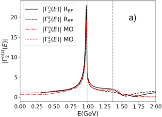
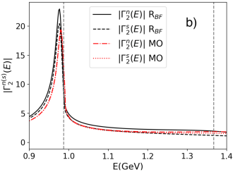
Figure 14: Moduli, a) for 0 GeV $\leqslant E\leqslant 2$ GeV and b) for 0.9 GeV $\leqslant E\leqslant~{}1.4$ GeV, of the isoscalar-scalar kaon form factors calculated using the Muskhelishvili-Omnès dispersion relation approach Moussallam_2019 . They are compared to those (continuous black lines) derived in the best fit in Sec. IV from a unitary relativistic three coupled-channel model. Both approaches use the updated $T_{\pi\pi}$ matrix derived in Appendix A. The physical $E$ region, 0.987 GeV $\lesssim E\lesssim$1.367 GeV, is delimited by the two vertical dashed lines.

In this appendix we complete our study by describing the results of two fits of the BABAR-Collaboration Dalitz-plot distribution B10 taking, in the amplitudes with final kaon-kaon states in $S$ wave and isospin 0, the scalar $K\overline{K}$ form factors derived from the Muskhelishvili-Omnès (MO) approach MO . The same parametrizations as those described in Sec. II are used for all other amplitudes. In the MO dispersion-relation framework the isoscalar-scalar $\Gamma_{2}^{n,s}(s)$ form factors have been calculated by B. Moussallam Moussallam_2000 ; Moussallam_2019 from the MO equation using the updated $\pi\pi$-$T$ matrix of the $\pi\pi$, $K\overline{K}$ and effective $(2\pi)(2\pi)$ coupled-channel model of Ref. EPJ (see Appendix A). In Fig. 14 the moduli of these MO form factors are compared to those derived in Sec. IV from a relativistic coupled-channel model. In Sec. II one has introduced for the form factors $\Gamma_{2}^{n,s}(s)$ complex phenomenological coefficients of proportionality $\chi^{n,s}$ and in Sec. IV, to achieve good fits, notably to reproduce the low density of events in the central region of the Dalitz distribution (see Fig. 8, region II), we have been led to multiply them by the energy-dependent phenomenological functions $P_{i}(s_{0})$ defined below in Eqs. (114) and (115).

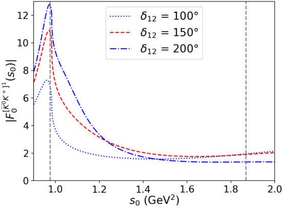
Figure 15: Moduli of the isovector-scalar kaon form factors calculated from MO equations in Ref. Bachir2015 for different $\delta_{12}$ parameters which correspond to the sum of the $\eta\pi\to\eta\pi$ and $K\bar{K}\to K\bar{K}$ phase shifts at $\sqrt{s}=m_{a_{0}(1450)}$. The two vertical dashed lines delimit the physical $s_{0}$ region, 0.975 GeV² $\lesssim s\lesssim$1.87 GeV².

The isovector-scalar $F_{0}^{[\overline{K}^{0}K^{+}]^{1}}(s)$ form factor has been calculated in Ref. Bachir2015 from coupled MO equations for $\pi\eta$ and $K\overline{K}$ channels. Its modulus, for the parameters $\delta_{12}$= 100^∘, 150^∘ and 200^∘ which are equal to the sum of the $\eta\pi\to\eta\pi$ and $K\bar{K}\to K\bar{K}$ phase shifts at $\sqrt{s}=m_{a_{0}(1450)}$ , is plotted in Fig. 15. The isovector amplitudes associated to the isospin-1 $a_{0}^{0}$ and $a_{0}^{+}$ resonances can be expressed in terms of this form factor by using, in the Eqs. (82) and (86), the relation (85) with $G_{1}(0)=\chi^{1}$. The strength $\chi^{1}$ is real and to obtain good fits, it was necessary to multiply it by the phenomenological polynomial

$$P_{F}(s_{+})\equiv 1+c_{1}(s_{+}-s^{\prime\prime})+c_{2}(s_{+}-s^{\prime\prime})^{2}+c_{3}(s_{+}-s^{\prime\prime})^{3},$$ (113)

where the free parameters $c_{i},\ i=1,2,3$ and $s^{\prime\prime}$ are real.

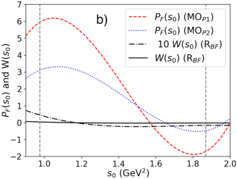
Figure 16: Comparison of: a) the functions $P_{i}(s_{0})$ multiplying, for the three models MO_P1, MO_P2 and R_BF, the isoscalar-scalar form factors $\Gamma_{2}^{n(s)}(s_{0})$; b) the polynomials $P_{F}(s_{0})$ multiplying, for the two models MO_P1(P2), the isovector-scalar form factor $F_{0}^{[\overline{K}^{0}K^{+}]^{1}}(s_{0})$ and $W(s_{0})$ introduced in Eq. (108) for the $G_{1}(s_{0})$ function of the best fit R_BF. Vertical dashed lines as in Fig. 15.

An estimation of the phenomenological strength parameters $\chi^{n,s}$ using Eq. (102) with $|\Gamma_{2}^{n,s}(m^{2}_{f_{0}})|\simeq~{}19$ (see Fig. 14) leads to $|\chi^{n,s}|\simeq 26\ \rm{GeV}^{-1}$. For the kaon isovector-scalar form factor with $\chi^{1}|F_{0}^{[\overline{K}^{0}K^{+}]^{1}}(m^{2}_{a_{0}})|={g_{a_{0}K^{+}K^{-}}}/[{m_{a_{0}}\,\Gamma_{tot}(a_{0})}]=89.66~{}\rm{GeV}^{-1}$, using (see Ref. AFLL ), $\Gamma_{tot}(a_{0})=71\pm 14$ MeV, $|g_{a_{0}K^{+}K^{-}}|^{2}/(4\pi)=0.275$ GeV², $m_{a_{0}}=980$ MeV and for $\delta_{12}=150^{\circ}$ $|F_{0}^{[\overline{K}^{0}K^{+}]^{1}}(m^{2}_{a_{0}})|\simeq 10.89$ (see Fig. 15), one obtains $\chi^{1}\simeq 8.2\rm\ {GeV}^{-1}$. As expected, from our study in Sec. III of the near threshold comparison between the $K^{+}K^{-}$ $S$-wave effective mass projection with that of the $\overline{K}^{0}K^{+}$, a good fit without the contribution associated with the isospin 0 $f_{0}$ resonances ($\chi^{n,s}\equiv 0$) cannot be obtained.

Table 11: Comparison between the MO_P1, MO_P2 parameters from the two fits using kaon scalar-form factors derived from dispersion relations (see the text) and the corresponding R_BF ones, from the best fit with kaon scalar-form factors calculated from unitary relativistic equation (see Table 2). The number of free parameters is denoted by $N_{p}$. Parameters without uncertainties are kept fixed during the minimization procedure. Phases $\varphi$ are in radians and detailed definitions of all parameters are given in the text.

Fit	MOP1	MOP2	RBF
$\chi^{2}(N_{p},\chi^{2}/ndf)$	1559.7(16, 1.32)	1546.9(16, 1.31)	1474.4(19, 1.25)
$|\chi^{n}|$(GeV${}^{-1})$	26.	35.	22.5
$\varphi_{\chi^{n}}$	1.63 ${}^{+0.20}_{-0.18}$	4.19 ${\pm 0.10}$	2.22${}^{+0.82}_{-0.98}$
$\chi^{s}$(GeV${}^{-1})$	26.	26.	22.5
$|F_{0}^{K^{0}f_{0}}(m_{D^{0}}^{2})|$	0.42${}^{+0.03}_{-0.04}$	0.35${\pm 0.03}$	2.22${}^{+0.26}_{-0.17}$
$\varphi_{F_{0}^{K^{0}f_{0}}}$	2.40${}^{+0.05}_{-0.04}$	1.94 ${\pm 0.05}$	2.21${\pm 0.10}$
$s^{\prime}$(GeV-2)	0.	-3.	1.56${}^{+0.02}_{-0.01}$
$s^{\prime\prime}$(GeV2)	1.5	1.5
$\chi^{1}$(GeV${}^{-1})$	8.2	15
$c_{1}$(GeV2)	-15.38 ${}^{+0.41}_{-0.45}$	-7.53 ${\pm 0.14}$
$c_{2}$(GeV-2)	8.16${}^{+0.66}_{-0.65}$	2.88${}^{+0.35}_{-0.34}$
$c_{3}$(GeV-4)	37.20 ${}^{+1.99}_{-1.94}$	18.24${}^{+0.91}_{-0.89}$
$|F_{0}^{K^{-}a^{+}}(m_{D^{0}}^{2})|$	0.23${\pm 0.01}$	0.28${\pm 0.01}$	0.25${}^{+0.02}_{-0.03}$
$\varphi_{F_{0}^{K^{-}a^{+}}}$	5.82${\pm 0.05}$	5.61${}^{+0.05}_{-0.04}$	5.33${}^{+0.12}_{-0.08}$
$|A_{0}^{K^{0}\phi}(m_{D^{0}}^{2})|$	0.99$\pm{0.01}$	0.99${\pm 0.01}$	0.99${\pm 0.01}$
$\varphi_{A_{0}^{K^{0}\phi}}$	-0.89${\pm 0.02}$	-0.97${\pm 0.02}$	3.67${}^{+0.12}_{-0.09}$
$M_{\phi}$(MeV)	1019.55$\pm 0.02$	1019.56$\pm 0.02$	1019.58$\pm 0.02$
$\Gamma_{\phi}$(MeV)	4.69$\pm$0.04	4.70$\pm$0.04	4.72$\pm$0.04
$|A_{0}^{K^{-}\rho^{+}}(m_{D^{0}}^{2})|$	5.78${}^{+0.22}_{-0.25}$	7.94${}^{+0.34}_{-0.37}$	$9.38^{+0.63}_{-0.58}$
$\varphi_{A_{0}^{K^{-}\rho^{+}}}$	1.18 $\pm{0.03}$	1.06${\pm 0.02}$	5.01${}^{+0.06}_{-0.05}$
$|P_{D}|$	15.71${}^{+0.78}_{-0.80}$	14.16${}^{+0.69}_{-0.70}$	$5.52^{+1.25}_{-1.24}$
$\varphi_{P_{D}}$	1.13$\pm{0.09}$	0.97${}^{+0.10}_{-0.09}$	3.97${}^{+0.23}_{-0.25}$

We also find that improved $\chi^{2}$ are obtained with the $\delta_{12}$ parameter of the isovector-scalar $F_{0}^{[\overline{K}^{0}K^{+}]^{1}}$ form factor equal to 150^∘ (see Fig. 15). With the $N_{p}$=16 free parameters displayed in Table LABEL:Tabparam, we obtain a fit, denoted as MO_P1, with a total $\chi^{2}$ of 1559.7 which corresponds to a $\chi^{2}/ndf$=1.32, not as good as that found in the best fit model of Sec. IV. In this fit, the phenomenological function multiplying the $\Gamma_{2}^{n(s)}(s_{0})$ is chosen to be

$$P_{1}(s_{0})\equiv P(s_{0}),$$ (114)

with the zero $s^{\prime}$ of the function $P(s_{0})$ [Eq. (103)] at 0 GeV². Fixing $|\chi^{n}|$ to 35 (GeV${}^{-1})$, $\chi^{1}$ to 15 (GeV${}^{-1})$ a slightly better fit, denoted MO_P2, with $N_{p}=16$ and a total $\chi^{2}$ of 1546.9 ($\chi^{2}/ndf$=1.31) is obtained with

$$P_{2}(s_{0})=1-s^{\prime}(s_{0}-s_{th}).$$ (115)

Table LABEL:Tabparam gives then a comparison of all parameter values with their uncertainties (when these parameters are fitted) for the MO_P1, MO_P2 models together with the corresponding parameters of the best fit R_BF presented in Sec. IV. The variations, in the $s_{0}$ physical region, of the different functions $P_{i}(s_{0})$ for the MO_P1 ($i=1,\ s^{\prime}=0$ GeV²) , MO_P2 ($i=2$,   $s^{\prime}=~{}{-3}$ GeV²) and R_BF ($i=1,\ s^{\prime}=1.56$ GeV^-2) fits are displayed in Fig. 16(a). As already indicated in Sec. IV [see second sentence below Eq. (108)] Fig. 16(b) compares the fitted polynomial $W(s_{0})$ to the phenomenological polynomials $P_{F}(s_{0})$ [see Eq. (113)] multiplying the isovector-scalar form factor $F_{0}^{[\overline{K}^{0}K^{+}]^{1}}(s_{0})$ for the two solutions MO_P1(P2).

Table 12: As in Table LABEL:Tabparam but for the branching fractions in percent of the amplitudes ${\cal{M}}_{i}$, $i=1$ to $7$. For each branching fraction we indicate the dominant resonances (see text) of the quasi-two-body channels of the different amplitudes (see Table 5). For the MO fits, the given uncertainties, $\Delta{\rm Br}_{i},i=1,7$ and of their sum are calculated from Eqs. (116) to (118) using the average positive and negative uncertainties of the free parameters displayed in Table LABEL:Tabparam. See Sec. IV for the calculation of the $\Delta{\rm Br}_{i}$ of the R_BF model. The uncertainties of the sum of the ${\rm Br}_{i}$ are obtained through the formula given in Eq. (118).

Fit	MOP1	MOP2	RBF
$\chi^{2}(N_{p},\chi^{2}/ndf)$	1559.7(16, 1.32)	1546.9(16, 1.31)	1474.4(19, 1.25)
${\rm Br}_{1}$[$f_{0}$’$s$, $a_{0}^{0}$’$s$]	44.9$\pm$8.3	63.0$\pm$ 15.8	$60.9^{+24.4}_{-10.6}$
${\rm Br}_{2}$[$\phi$]	44.9$\pm$0.5	44.8$\pm$ 0.5	45.5$\pm$ 0.7
${\rm Br}_{3}$[$a_{0}^{+}$’$s$]	25.9$\pm$ 0.8	40.1$\pm$1.9	$20.7^{+9.4}_{-6.0}$
${\rm Br}_{4}$[$\rho^{+}$’$s$]	7.7$\pm$ 0.6	13.1 $\pm$1.2	$21.5^{+3.1}_{-2.8}$
${\rm Br}_{5}$[$a_{0}^{-}$’$s$]	2.6$\pm$ 0.1	2.7$\pm$ 0.1	$0.76^{+0.18}_{-0.15}$
${\rm Br}_{6}$[$\rho^{-}$’$s$]	0.03$\pm$0.002	0.06$\pm$ 0.005	0.08$\pm$ 0.01
${\rm Br}_{7}$[$f_{2}(1270)$]	0.37$\pm$ 0.04	0.30$\pm$ 0.03	0.05$\pm$0.02
$\sum_{i=1,7}{\rm Br}_{i}$	126.3$\pm$7.6	164.1$\pm$ 13.7	149.5${}^{+26.9}_{-12.3}$

The different branching fractions Br${}_{i},i=1$ to 7, of these two fits are compared to those of the best fit model in Table LABEL:TabBr45Req. Following Eq. (98) their given uncertainties $\Delta{\rm Br}_{i}$ are calculated as

$$\Delta{\rm Br}_{i}=\frac{1}{32(2\pi)^{3}m_{D^{0}}^{3}\Gamma_{D^{0}}}\left[\sum_{k,l=1,N_{p}}\frac{\partial f_{i}}{\partial r_{k}}\ \frac{\partial f_{i}}{\partial r_{l}}\ \rho_{kl}\ \Delta r_{k}\ \Delta r_{l}\right]^{1/2}$$ (116)

where,

$$\frac{\partial f_{i}}{\partial r_{k}}=\int\int ds_{+}ds_{0}\ 2\left(R_{i}\frac{\partial R_{i}}{\partial r_{k}}+I_{i}\frac{\partial I_{i}}{\partial r_{k}}\right)\ \rm{with}\ f_{i}=\int\int ds_{+}ds_{0}\ |{\cal M}_{i}(s_{0},s_{+})|^{2},$$ (117)

and ${\cal M}_{i}=R_{i}+i\ I_{i}$. In Eqs. (116) and (117) $r_{k(l)}$ are the free parameters entering the amplitude ${\cal M}_{i}$. In Eq. (116), $\Delta r_{k(l)}$ are the $r_{k(l)}$ average uncertainties and $\rho_{kl}$ are the $kl$ correlation coefficients of the MINUIT program. These quantities are given in the minimization output with $\rho_{kl}=\rho_{lk}$ and $\rho_{kl}=1$ if $k=l$. The uncertainty $\Delta$Br of the sum of the Br_i is calculated as

$$\Delta{\rm Br}=\frac{1}{32(2\pi)^{3}m_{D^{0}}^{3}\Gamma_{D^{0}}}\left[\sum_{i,j=1,7}\left(\sum_{k,l=1,N_{p}}\frac{\partial f_{i}}{\partial r_{k}}\ \frac{\partial f_{j}}{\partial r_{l}}\ \rho_{kl}\ \Delta r_{k}\ \Delta r_{l}\right)\right]^{1/2}.$$ (118)

The branching fractions of the three components of the ${\cal{M}}_{1}$ amplitude, viz., ${\cal{M}}^{n,I=0}_{1}$, ${\cal{M}}^{s,I=0}_{1}$, ${\cal{M}}^{I=1}_{1}$ [see Eqs. (79)-(82)], given in Table LABEL:TabBr45Reqa show that the isoscalar $f_{0}$ and isovector $a_{0}^{0}$ resonance contributions can be quite different. However, taking into account the large uncertainties in the Br₁ values of the MO_P1, MO_P2 and R_BF fits (see Table LABEL:TabBr45Req) the total scalar-resonance contribution in the ${\cal{M}}_{1}$ amplitude is similar. The corresponding results can be qualitatively interpreted from, the expressions of the amplitudes given in Sec. II.4, the values of the different parameters given in Tables 2, LABEL:Tabparam and those of the kaon scalar-form factors in use. For the three terms of the ${\cal M}_{1}$ amplitude [see Eqs. (79)-(82)] one can define the renormalized amplitudes,

$${\overline{\cal{M}}}^{n,I=0}_{1}(s_{0})=\frac{{{\cal{M}}}^{n,I=0}_{1}(s_{0})}{F_{W}},\ \ \ {\overline{\cal{M}}}^{s,I=0}_{1}(s_{0})=\frac{{{\cal{M}}}^{s,I=0}_{1}(s_{0})}{F_{W}}\ \ \ {\rm and}\ \ \ {\overline{\cal{M}}}^{I=1}_{1}(s_{0})=\frac{{{\cal{M}}}^{I=1}_{1}(s_{0})}{F_{W}},$$ (119)

where $F_{W}=-G_{F}\ (\Lambda_{1}+\Lambda_{2})\ a_{2}/2$. In the case of the amplitude ${\cal{M}}_{3}(s_{+})$ [see Eq. (86)], with $F^{\prime}_{W}=G_{F}\ \Lambda_{1}\ a_{2}/2$, one define the renormalized amplitude

$${\widetilde{\cal{M}}}_{3}(s_{+})=\frac{{\cal{M}}_{3}(s_{+})}{F^{\prime}_{W}}.$$ (120)

The coupling $\Lambda_{2}$ (=$-0.05)$ is small and $\Lambda_{1}+\Lambda_{2}$ (=0.90) is close to $\Lambda_{1}$ (=0.95) [see Eq. (2)], consequently $F^{\prime}_{W}$ is close to $F_{W}$. One can then compare the amplitudes (119) and (120) because the contribution of the $a_{1}$ term in ${\cal{M}}_{3}(s_{+})$ is negligible since the factor $m_{K}^{2}-m_{K^{0}}^{2}=-0.0039$ GeV² is very small. The moduli of these amplitudes are plotted, for the best fit as the black continuous lines denoted by R_BF, the red dashed curve for the MO_P1 model and the blue dotted one for the MO_P2 one, in Figs. 17(a), (b), (c) and (d).

The comparison, shown in Fig. 17, of the resulting $s_{0}$ behavior of the moduli $|{\overline{\cal{M}}}^{n,I=0}_{1}(s_{0})|$, $|{\overline{\cal{M}}}^{s,I=0}_{1}(s_{0})|$ and $|{\overline{\cal{M}}}^{I=1}_{1}(s_{0})|$ allows furthermore to understand qualitatively the different branching fractions displayed in Table LABEL:TabBr45Reqa. The branching fractions can also be partly compared to the fit fractions of the BABAR isobar-model experimental analysis supmaPRL105 .

The dominance of the branching fraction associated to the isoscalar-scalar amplitude ${\cal M}_{1}^{s,I=0}$ for the best fit and to a less extent for the MO_P1 one, can be understood as their moduli $|{\overline{\cal{M}}}^{s,I=0}_{1}(s_{0})|$ [Fig. 17(b)] are larger than the moduli $|{\overline{\cal{M}}}^{n,I=0}_{1}(s_{0})|$ [Fig. 17(a)] and $|{\overline{\cal{M}}}^{I=1}_{1}(s_{0})|$ [Fig. 17(c)]. Comparison of Fig. 17(a) and Fig. 17(c) can also explain qualitatively, for the best fit, the difference between the ${\cal M}_{1}^{n,I=0}$ (1.19%) and ${\cal M}_{1}^{I=1}$ (4.48%) branching fractions.

Table 13: As in Table LABEL:Tabparam but for the branching fractions in percent of the amplitudes ${\cal{M}}^{n,I=0}_{1}$, ${\cal{M}}^{s,I=0}_{1}$ and ${\cal{M}}^{I=1}_{1}$ [see Eqs. (79-82)]. Lines 8 to 10 give the contribution of the interferences between these amplitudes.

Fit	MOP1	MOP2	RBF
$\chi^{2}(N_{p},\chi^{2}/ndf)$	1559.7(16, 1.32)	1546.9(16, 1.31)	1474.4(19, 1.25)
${\rm Br}_{1}$[$f_{0},a_{0}^{0}$]	44.88	63.01	60.93
${\rm Br}[{\cal{M}}^{n,I=0}_{1}$: $f_{0}$ in $\Gamma^{n}(s)$]	4.75	20.66	1.19
${\rm Br}[{\cal{M}}^{s,I=0}_{1}$: $f_{0}$ in $F_{0}^{K^{0}f_{0}}(m_{D^{0}}^{2})$ $\Gamma^{s}(s)$]	22.69	45.91	59.82
${\rm Br}[{\cal{M}}^{I=1}_{1}$: $a_{0}^{0}$ in $\chi^{1}P_{F}(s)$ $F_{0}^{[\overline{K}^{0}K^{+}]^{1}}(s)\ {\rm or}\ G_{1}(s)$]	16.47	16.47	4.48
${\rm Br}({\cal{M}}^{n,I=0}_{1})+{\rm Br}({\cal{M}}^{s,I=0}_{1})+{\rm Br}({\cal{M}}^{I=1}_{1})$	43.90	83.04	65.49
2 ${\rm Br}_{1112}$	-12.95	-37.98	-14.6
2 ${\rm Br}_{1113}$	1.86	16.44	-0.72
2 ${\rm Br}_{1213}$	12.03	0.43	10.8
$\sum_{i,j=1,3}^{i\neq j}{\rm Br}_{1i1j}$	0.94	-20.02	-4.57

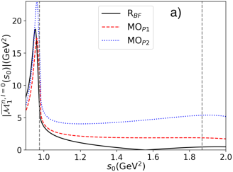
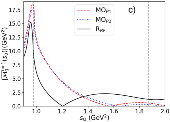
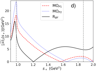
Figure 17: The black continuous line, denoted by R_BF represents in a) $|{\overline{\cal{M}}}^{n,I=0}_{1}(s_{0})|$, in b) $|{\overline{\cal{M}}}^{s,I=0}_{1}(s_{0})|$, and in c) $|{\overline{\cal{M}}}^{I=1}_{1}(s_{0})|$ [see Eqs. (119)] and in d) $|{\widetilde{\cal{M}}}_{3}(s_{+})|$ [see Eq. (120)]. The red dashed curve, the blue dotted one represent the corresponding moduli for the alternative MO_P1, MO_P2 fits, respectively. As in Fig. 15 for the two vertical dashed lines (the $s_{+}$ limits are very close to the $s_{0}$ ones)

.

For the $S$-wave $K\overline{K}$ contributions there are important differences between the models MO_P1, MO_P2 and R_BF. The kaon isoscalar-scalar form factors are similar (see Figs. 9 and 14) but multiplication by the function $P_{i}(s_{0})$ [see Eqs. (103), (114 and (115)] implies different modifications. For the MO fits, the kaon isovector-scalar form factor $F_{0}^{[\overline{K}^{0}K^{+}]^{1}}(s_{0})$ is multiplied by different phenomenological polynomials $P_{F}(s_{0})$ [Eq. (113)] compared, in the Fig. 16(b), to the fitted polynomial $W(s_{0})$ [Eq. (108)] entering the $G_{1}(s_{0})$ function of the best fit.

In the MO_P2 fit (${\rm Br}({\cal{M}}^{n,I=0}_{1})$= 20.66 %) the $f_{0}$ contribution in $\Gamma_{2}^{n}(s)$ is enhanced by a larger $|\chi^{n}|$ (35 GeV^-1) and by the function $P_{1}(s_{0})$ while it is more suppressed in the best fit (1.19 %) than in the MO_P1 one (4.75 %).

A striking difference arises for the modulus of the phenomenological transition form factor $F_{0}^{K^{0}f_{0}}(m_{D^{0}}^{2})$: it is quite large, 2.22, for the best fit solution R_BF as compared to its magnitude for the two other fits where it is smaller than 0.43. This leads to large value of the branching fraction (59.82 %) for the ${\cal{M}}^{s,I=0}_{1}(s_{0})$ amplitude arising from $D^{0}$ annihilation via $W$ exchange in the R_BF best fit solution (see Table LABEL:TabBr45Reqa). The $|\chi^{s}|$ being the same (26 GeV^-1), the difference between the MO_P1 (22.69 %) and MO_P2 (45.91 %) branching fractions arises from smaller $P_{1}(s_{0})$ enhancement (for $s_{0}\gtrsim 1.3$ GeV²) than that of $P_{2}(s_{0})$, as can be seen in Figs. 16(a) and 17(b).

The values of the ${\rm Br}({\cal{M}}^{I=1}_{1})$ in the fith line of Table LABEL:TabBr45Reqa indicate the isospin-1 $a_{0}^{0}$ resonances content in $\chi_{1}P_{F}(s)F_{0}^{[\overline{K}^{0}K^{+}]^{1}}$ or $G_{1}(s)$. This branching fraction small (4.48 %) in the R_BF fit (some suppression because of $W(s_{0})$) is the same (16.47 %) in the MO_P1 and MO_P2, the larger $P_{F}(s_{0})$ [Fig. 16(b)] is conpensated by a smaller $\chi^{1}$ (8.2 versus 15).

The branching fraction Br₃, which indicates the isovector $a_{0}^{+}$ resonances contribution, has values of 25.9, 40.1 and 20.7 % for the MO_P1, MO_P2 and R_BF fits, respectively (see Table LABEL:TabBr45Req). The modulus of the transition form factor $F_{0}^{K^{-}a_{0}^{+}}(m_{D^{0}}^{2})$, entering in Eq. (86) is equal to 0.23, 0.28 and 0.25 for the MO_P1, MO_P2 and best fits, respectively. The branching fractions depend on the $\chi^{1}$ values and $P_{F}(s_{+})$ behavior for the MO fits and on the role of $G_{1}(s_{+})$ in the R_BF solution and their values are in qualitative agreement with the corresponding $|{\widetilde{\cal{M}}}_{3}(s_{+})|$ curves shown in Fig. 17(d).

The role of the $[\rho(770)^{+}+\rho(1450)^{+}+\rho(1700)^{+}]$ resonances is different in our models: the Br₄ of the MO_P1, MO_P2 and R_BF fits are equal to 7.7, 13.1 and 21.5 %, respectively (see Table LABEL:TabBr45Req). The large contribution in the R_BF solution is partly due to the magnitude, 9.38, of the modulus of the transition form factor $|A_{0}^{K^{-}\rho^{+}}(m_{D^{0}}^{2})|$ to be compared to 5.78 and 7.94 for the MO_P1 and MO_P2 fits, respectively. The Br₄ ratio between that of the R_BF and those of the MO_P1 and MO_P2 fits is close to the square of the corresponding $|A_{0}^{K^{-}\rho^{+}}(m_{D^{0}}^{2})|$ ratios. It can be seen that, to improve the $\chi^{2}$ of the fits, it seems necessary to increase the $\rho^{+}$ resonances contributions.

The small isospin-1 $a_{0}^{-}$ and $\rho^{-}$ resonances contents in ${\rm Br_{5(6)}}$ come from the fact that the ${\cal M}_{5(6)}$ amplitudes [see Eqs. (88) and (89)] are proportional to the $V_{CKM}$ coupling $\Lambda_{2}$ with $|\Lambda_{2}/\Lambda_{1}|~{}\simeq~{}5~{}\times~{}10^{-2}$, while all other amplitudes are proportional either to $\Lambda_{1}+\Lambda_{2}$ [${\cal M}_{1}$, Eq. (79) with Eqs. (80), (81), (82), ${\cal M}_{2}$, Eq. (83) and ${\cal M}_{7}$, Eq. (91)] or to $\Lambda_{1}$ [${\cal M}_{3}$ Eq. (86) and ${\cal M}_{4}$, Eq. (87)].

The $f_{2}(1270)$ resonance contributions in Br₇ for our three fits follow the evolution of the square of the $|P_{D}|$ parameter in each fit. They are very small and even smaller than in the BABAR analysis supmaPRL105 .

The negative total interference contributions are equal to -26.3 %, -64.1 % and -49.5 %, for the MO_P1, MO_P2 and R_BF fits, respectively, compared to that of the isobar BABAR model of -63.4 % supmaPRL105 .

The comparison of the off-diagonal elements ${\rm Br}_{ij}$, $i\neq j$ shows large interferences between the amplitudes giving large or sizable branching fractions (see for instance Table 6 of the best fit). This is in particular the case between ${\cal M}_{1}(s_{0})$ and ${\cal M}_{4}(s_{+})$. These values can be qualitatively expected by inspecting the different branching fractions given in Table LABEL:TabBr45Req.

References

- (1) A. Zupanc et al. (Belle Collaboration), Measurement of in meson decays to the final state, Phys. Rev. D 80, 052006 (2009).
- (2) P. del Amo Sanchez et al. (BABAR Collaboration), Measurement of Mixing Parameters Using and Decays, Phys. Rev. Lett. 105, 081803 (2010).
- (3) B. Aubert et al. (BABAR Collaboration), Dalitz plot analysis of , Phys. Rev. D 72, 052008 (2005).
- (4) B. Aubert et al. (BABAR Collaboration), Improved measurement of the CKM angle in decays with a Dalitz plot analysis of D decays to and , Phys. Rev. D 78, 034023 (2008).
- (5) Supplemental Material of P. del Amo Sanchez et al. (BABAR Collaboration), Measurement of Mixing Parameters Using and Decays, Phys. Rev. Lett. 105, 081803 (2010), http://link.aps.org/supplemental/10.1103/PhysRevLett.105.081803) and F. Martinez-Vidal (private communication).
- (6) P. Weidenkaff, Analysis of the decay with the BESIII experiment, Ph.D. thesis, Mainz University, 2016.
- (7) M. Abilikim et al. (BESIII Collaboration), Analysis of the decay , arXiv: 2006.02800.
- (8) P. del Amo Sanchez et al. (BABAR Collaboration), Evidence for Direct CP Violation in the Measurement of the Cabbibo-Kobayashi-Maskawa Angle with Decays, Phys. Rev. Lett. 105, 121801 (2010).
- (9) A. Poluektov et al. (Belle Collaboration), Evidence for direct CP-violation in the decay , and measurement of the CKM phase , Phys. Rev. D 81, 112002 (2010).
- (10) J. P. Lees et al. (BABAR Collaboration), Observation of direct CP violation in the measurement of the Cabibbo-Kobayashi-Maskawa angle with decays, Phys. Rev. D 87, 052015 (2013).
- (11) R. Aaij et al. (LHCb Collaboration), Measurement of CP violation and constraints on the CKM angle in with decays, Nucl. Phys. B888, 169 (2014).
- (12) J. Libby et al. (CLEO Collaboration), Model-independent determination of the strong-phase difference between and and its impact on the measurement of the CKM angle , Phys. Rev. D 82, 112006 (2010).
- (13) H. Aihara et al. (Belle Collaboration), First measurement of with a model-independent Dalitz plot analysis of decay, Phys. Rev. D 85, 112014 (2012).
- (14) R. Aaij et al. (LHCb Collaboration), Measurement of the CKM angle using with , decays, J. High Energy Phys. 08 (2018) 176.
- (15) M. Abilikim et al. (BESIII Collaboration), Improved model-independent determination of the strong-phase difference between and decays, arXiv:2007.07959v1.
- (16) J.-P. Dedonder, R. Kamiński, L. Leśniak and B. Loiseau, Dalitz plot studies of decays in a factorization approach, Phys. Rev. D 89, 094018 (2014).
- (17) D. Boito, J.-P. Dedonder, B. El-Bennich, R. Escribano, R. Kamiński, L. Leśniak, and B. Loiseau, Parametrizations of three-body hadronic - and -decay amplitudes in terms of analytic and unitary meson-meson form factors, Phys. Rev. D 96, 113003 (2017).
- (18) J.-P. Dedonder, A. Furman, R Kamiński, L. Leśniak and B. Loiseau, Final state interactions and CP violation in decays, Acta Phys. Pol. B 42, 2013 (2011).
- (19) A. Furman, R. Kamiński, L. Leśniak, and P. Żenczykowski, Final state interactions in decays, Phys. Lett. B 699, 102 (2011).
- (20) L. Leśniak and P. Żenczykowski, Dalitz-plot dependence of asymmetry in decays, Phys. Lett. B 737, 201 (2014).
- (21) R. Kamiński, L. Leśniak, and B. Loiseau, Three channel model of meson-meson scattering and scalar meson spectroscopy, Phys. Lett. B 413, 130 (1997).
- (22) R. Kamiński, L. Leśniak, and B. Loiseau, Scalar mesons and multichannel amplitudes, Eur. Phys. J. C 9, 141 (1999).
- (23) A. Furman, and L. Leśniak, Coupled channel study of resonances, Phys. Lett. B 538, 266 (2002).
- (24) A. Furman, and L. Leśniak, Properties of the resonances, Nucl. Phys. B (Proc. Suppl.) 121, 127 (2003).
- (25) C. Bruch, A. Khodjamirian, and J. H. Kühn, Modeling the kaon form factors in the timelike region, Eur. Phys. J. C. 39, 41 (2005).
- (26) P. A. Zyla et al. (Particle Data Group), Review of particle physics, Prog. Theor. Exp. Phys. 2020, 083C01 (2020).
- (27) N. I. Muskhelishvili, in Singular integral equations (P. Noordhoff Ltd., Gr^ningen, The Netherlands 1953), Chaps; 18 and 19; R. Omnès, On the solution of certain singular integral equations of quantum field theory, Nuovo Cimento 8, 316 (1958).
- (28) B. Moussallam, dependence of the quark condensate from a chiral sum rule, Eur. Phys. J. C 14, 111 (2000) and private communication.
- (29) B. Moussallam, (private communication).
- (30) M. Albaladejo and B. Moussallam, Form factors of the isoscalar-scalar current and the phase shifts, Eur. Phys. J. C 75, 488 (2015).
- (31) G. Buchalla, A. J. Buras and M. E. Lautenbacher, Weak decays beyond leading logarithms, Rev. Mod. Phys. 68, 1125 (1996).
- (32) A. J. Buras, QCD factors and beyond leading logarithms versus factorization in non leptonic heavy meson decays, Nucl. Phys. B434, 606 (1995).
- (33) A. Ali, G. Kramer, and Cai-Dian Lü, Experimental tests of factorization in charmless nonleptonic two-body B decays, Phys. Rev. D 58, 094009 (1998).
- (34) M. Beneke and M. Neubert, QCD factorization for and decays, Nucl. Phys. B675, 333 (2003).
- (35) B. El-Bennich, O. Leitner, J.-P. Dedonder, and B. Loiseau, Scalar meson in heavy-meson decays, Phys. Rev. D 79, 076004 (2009).
- (36) D. Melikhov, Dispersion approach to quark-binding effects in weak decays of heavy mesons, Eur. Phys. J. direct 4, 1 (2002).
- (37) B. Aubert et al. (BABAR Collaboration), Amplitude analysis of the decay , Phys. Rev. D 76, 011102(R) (2007).
- (38) P. del Amo Sanchez et al. (BABAR Collaboration), Dalitz plot analysis of , Phys. Rev. D 83, 052001 (2011).
- (39) P. Ball and G.W. Jones, Twist-3 distribution amplitudes of K* and phi Mesons, J. High Energy Phys. 03 (2007) 069.
- (40) S. Baker, R.D. Cousins, Clarification of the use of and likelihood functions in fits to histograms, Nucl. Instrum. Methods Phys. Res. 221, 437 (1984).
- (41) A. Furman, R. Kamiński, L. Leśniak, and B. Loiseau, Long-distance effects and final state interactions in and decays, Phys. Lett. B 622, 207 (2005).
- (42) L. Leśniak, Meson spectroscopy and separable potentials, Acta Phys. Pol. B 27, 1835 (1996), https://www.actaphys.uj.edu.pl/R/27/8/1835/pdf.
- (43) Y. Nakahama et al. (Belle Collaboration), Measurement of CP violating asymmetries in decays with a time-dependent Dalitz approach, Phys. Rev. D 82, 073011 (2010).
- (44) J. P. Lees et al. (BABAR Collaboration), Study of CP violation in Dalitz-plot analyses of and , Phys. Rev. D 85, 112010 (2012).
- (45) J.R. Batley et al. (NA48/2 Collaboration), Precise tests of low energy QCD from decay properties, Eur. Phys. J. C 70, 635 (2010).
- (46) B. Moussallam (private communication).
- (47) R. Kamiński, L. Leśniak, K. Rybicki, Separation of the -wave pseudoscalar and pseudovector amplitudes in reaction on polarized target, Z. Phys. C 74, 79 (1997).
- (48) D. Cohen et al., Amplitude analysis of the system produced in the reaction at 6 GeV/c, Phys. Rev. D 22, 2595 (1980).
- (49) A. Etkin et al., Amplitude analysis of the system produced in the reaction at 23 GeV/c, Phys. Rev. D 25, 1786 (1982).