Detecting Security Fixes in Open-Source Repositories
using Static Code Analyzers
[PRE-PRINT]

Therese Fehrer, Rocío Cabrera Lozoya, Antonino Sabetta,

Dario Di Nucci, Damian A. Tamburri

The sources of reliable, code-level information about vulnerabilities that affect open-source software (OSS) are scarce, which hinders a broad adoption of advanced tools that provide code-level detection and assessment of vulnerable OSS dependencies.

In this paper, we study the extent to which the output of off-the-shelf static code analyzers can be used as a source of features to represent commits in Machine Learning (ML) applications. In particular, we investigate how such features can be used to construct embeddings and train ML models to automatically identify source code commits that contain vulnerability fixes.

We analyze such embeddings for security-relevant and non-security-relevant commits, and we show that, although in isolation they are not different in a statistically significant manner, it is possible to use them to construct a ML pipeline that achieves results comparable with the state of the art.

We also found that the combination of our method with commit2vec represents a tangible improvement over the state of the art in the automatic identification of commits that fix vulnerabilities: the ML models we construct and commit2vec are complementary, the former being more generally applicable, albeit not as accurate.  

Citing this paper

Please cite this work as:

@misc{fehrer2021detecting,

  title  = {Detecting Security Fixes in Open-Source Repositories

            using Static Code Analyzers},

  author = {Therese Fehrer and Roc\’io Cabrera Lozoya and Antonino Sabetta

            and Dario Di Nucci and Damian A. Tamburri },

  year   = {2021},

  month  = {March},

}

 

Abstract.

The sources of reliable, code-level information about vulnerabilities that affect open-source software (OSS) are scarce, which hinders a broad adoption of advanced tools that provide code-level detection and assessment of vulnerable OSS dependencies.

In this paper, we study the extent to which the output of off-the-shelf static code analyzers can be used as a source of features to represent commits in Machine Learning (ML) applications. In particular, we investigate how such features can be used to construct embeddings and train ML models to automatically identify source code commits that contain vulnerability fixes.

We analyze such embeddings for security-relevant and non-security-relevant commits, and we show that, although in isolation they are not different in a statistically significant manner, it is possible to use them to construct a ML pipeline that achieves results comparable with the state of the art.

We also found that the combination of our method with commit2vec represents a tangible improvement over the state of the art in the automatic identification of commits that fix vulnerabilities: the ML models we construct and commit2vec are complementary, the former being more generally applicable, albeit not as accurate.

1. Introduction

The adoption of open-source software (OSS) components in commercial products has dramatically increased over the past two decades. The large majority of commercial software products nowadays rely, to some extent, on open-source software (OSS) components (Zaffar et al., 2011). A study by Snyk (Tal, 2019) reports that the large majority of the applications they analyzed contained at least one open-source component; as much as 50% to the entire code-base of those applications is open-source. Whereas traditionally software vendors used to have full control on the entire development process of most of the components that made up their products, nowadays a large part of the codebases of those products come from community-developed free open-source projects, managed by independent parties (Pashchenko et al., 2021). By building upon these free, community-developed building blocks, vendors can focus their efforts on differentiating features bring them to the market faster. When doing so, however, they become responsible for assessing and mitigating the impact that a vulnerability in those open-source components might have on their products.

Advanced state-of-the-art tools such as Eclipse Steady use code-level information about the vulnerable code fragment and its fix; this enables efficient detection of vulnerable dependencies, as well as accurate impact assessment through reachability analysis (Ponta et al., 2020). To do so, Eclipse Steady relies on the availability of accurate data about the code-level changes (commits) that fix each known vulnerability.

Unfortunately, the data about security vulnerabilities is scattered across heterogeneous sources, often not machine readable, and do not provide the necessary level of detail, especially when it comes to code-level details. The NVD would the natural candidate to provide such information, but as shown in previous research (Schryen, 2011) one cannot rely on NVD advisories to find fix commits. Explicit mentions of CVE identifiers in commit messages are not frequent either (in our dataset, only 12.18% of the vulnerabilities have at least one fix commit that can be found by searching for the CVE identifier in the commit messages). Some attempts at curating vulnerability datasets do provide the necessary level of details, but they suffer from scalability issues because they are based on manual effort (Ponta et al., 2019).

This difficulty in obtaining accurate (code-level) vulnerability data hinders further development of new tools that could push the state of the art in vulnerability detection and mitigation. Also, it makes it harder for the research community to learn from real-world vulnerability and their fixes.

In this perspective, the role of automated tools to find vulnerability fixes in code repositories, possibly using machine learning, becomes increasingly important (Sabetta and Bezzi, 2018; Cabrera Lozoya et al., 2021). However, the research that is necessary to come up with such tools requires, in turn, a large amount of training data, which leads to a somewhat circular problem.

In this paper we present an approach to analyze repositories considering the changes introduced by individual commits. Instead of leveraging specialized representations (such as syntax trees, call graphs, data flow graphs, or their combinations) (Ghaffarian and Shahriari, 2017; Cabrera Lozoya et al., 2021), we investigate the use of off-the-shelf tools for code quality analysis to as sources of features to represent code changes as captured in commits. Based on representations build from these features, we train models to predict whether a commit is likely to fix a vulnerability or not. Static code analyzers have been combined with machine learning techniques for a range of other software engineering-related prediction tasks. They have been used in the context of software fault prediction (Malhotra, 2015; Li et al., 2018), defect prediction (Zimmermann and Nagappan, 2008; Premraj and Herzig, 2011; Tosun et al., 2009; Bhattacharya et al., 2012), code smell prediction (Lujan et al., 2020) and for the prediction and prioritization of technical debt (Codabux and Williams, 2016). We propose a model to represent code changes for whole repositories using static code analyzers. Based on this representation, we then use machine learning techniques to identify security-relevant commits and evaluate our model’s performance on an industrial dataset of vulnerabilities and their patches. The analysis of the differences between security-relevant and non-security-relevant commits reveals no statistically significant difference. Machine learning models leveraging the results of static analysis tools achieve results comparable with commit2vec. However, the latter is executable only on compilable code, being based on Abstract Syntax Trees. Overall, a model combining both approaches achieves better performance than those obtained by the approaches independently.

Our contributions are relevant from both an academic and an industrial perspective. In particular, we provide:

• new insights concerning the usage of off-the-shelf static code analyzer as sources of features that can be used to predict security-relevant commits;

• an extensible pipeline on to pre-process and combine the outputs of various static code analyzers to train machine learning models on commits;

• a comprehensive empirical study that compares models trained on such features with alternative, state-of-the-art, methods that use information extracted from abstract syntax trees.

Our approach is relevant to industry as it is applicable to a much broader range of commits than commit2vec (Cabrera Lozoya et al., 2021), the state-of-the-art tool for this task, leveraging on the combination of different static code analyzers. Our method can complement commit2vec yielding a tangible contribution to the goal of automating the identification of security-relevant commits (i.e., commits that fix vulnerabilities).

Outline

The remainder of this paper is structured as follows. Section 2 presents background information on software vulnerabilities and static code analyzers. Section 3 provides the goals of the empirical study and the data preparation steps. Section 4 describes how to extract embedding resulting from the output of the static code analyzer. Then, it analyzes the relationship between the embedding resulting from the output of the static code analyzer and the security-relevant commit. Section 5 introduces the pipeline to train the prediction models and the method adopted to evaluate them. It investigates and contrasts several machine-learning models and ensemble techniques. Finally, it compares the obtained results with those achieved by commit2vec. The threats to the validity of the empirical study are reported in Section 6, while Section 7 discusses the related literature. Finally, Section 8 concludes the paper and outlines the future work.

2. Background

The background of this research concerns software vulnerabilities and static analyzers, which we introduce in this section.

2.1. Software Vulnerabilities

Two of the most important institutions in the security ecosystem are the national vulnerability database (NVD) and Common Vulnerabilities and Exposures (CVE). The former is a U.S. government repository of vulnerability management data based on the CVE list and performs analysis on the vulnerabilities. The latter is a list of known cybersecurity documented vulnerabilities, which include their identification numbers and descriptions. It has become the standard for vulnerability and exposure identifiers.

CVE defines a vulnerability as “a flaw in software, firmware, hardware, or service component resulting from a weakness that can be exploited, causing a negative impact to the confidentiality, integrity, or availability of an impacted component or components”. In practice, different definitions of vulnerabilities are used, depending on the context and use case. This research originated from an industrial context through cooperation with SAP. The definition of vulnerabilities is driven by practical considerations about the availability of relevant data sources. We follow the definition of vulnerability presented in commit2vec (Cabrera Lozoya et al., 2021) since our research is based on the same industrial data set, where the vulnerabilities are implicitly defined through their associated fixes.

Once a vulnerability is identified, a patch is created and made available to the public (Frei et al., 2010). Software users need to install patches timely to minimize the time that they are under the risk of exploitation through the vulnerability. Commits that fix vulnerabilities are categorised as security-relevant commits.

2.2. Static Code Analyzers

Static analyzers read a program and construct its abstract representation without executing it (Louridas, 2006) to analyze its quality. Static analyzers rely on pattern matching, software metrics, and program analysis. In the context of our research, we identified four static analyzers to generate embeddings for the commits in our dataset.

Static Code Analyzed based on Pattern Matching

PMD and Checkstyle are source code analyzers designed to find common programming flaws and help to enforce coding standards. Developers can use the standard rule sets provided or create their own. In this way, the tools can be customized to fit different coding standards. PMD currently supports eight different programming languages, including Java and Apex. The standard ruleset for Java can detect eight bug categories. Checkstyle is focused on Java code only and provides two configuration files, which refer to the Sun Code conventions and the Google Java style, which are available as predefined styleguides. Both PMD and Checkstyle have been used previously used to detect code smells (Lujan et al., 2020). Lujan et al. (Lujan et al., 2020) employs also FindBugs. However, both FindBugs and its successor SpotBugs have the limitation of working with bytecode rather than source code. Therefore, we did not consider them for this research. There does, however, exist an extension for SpotBugs, which is called Find Security Bugs and is focused on security-related warnings. Future research might want to evaluate if these security-related bugs serve as a better feature set for training models to identify security-relevant commits.

Static Code Analyzed based on Software Metrics

CK extracts class- and metric-level code metrics from Java source code. It calculates 30 different types of metrics, including five out of the six CK metrics (Chidamber and Kemerer, 1994). The tool covers all CK metrics except the number of children (NOC), which was excluded due to memory issues. Please consider that the CK metrics have been used for various prediction tasks in software engineering, such as software fault prediction (Malhotra, 2015; Di Nucci et al., 2017; Li et al., 2018).

Static Code Analyzed based on Program Analysis

This category of static analyzers captures the inherent rich structure of source code.Progex ((Program Graph Extractor) extracts various graph representations like abstract syntax trees (ASTs), control flow graphs (CFGs), and program dependency graphs (PDGs) from source code. It is based on the ANTLR parser generator and currently supports only Java.

3. Empirical Study Goals and Data Preparation

The empirical study aims to understand to what extent machine learning classifiers can leverage static code analyzers to automatically identify security-relevant commits. These tools are widely used in the software development process and create numerical representations of source code. However, using such tools to create embeddings for commits has not been sufficiently explored so far.

RQ1. To what extent embedding resulting from static code analyzers can distinguish security-relevant commits?

One of the main challenges to apply machine techniques to detect security-relevant commits is numerically representing them. Embedding commit features means projecting the original feature space of the commits onto another feature space, which should ideally capture the most relevant information of the data points. Therefore, we aim at verifying to what extent static code analyzers can be used to create embeddings for commits, which significantly distinguish security-relevant commits.

RQ2. To what extent machine learning models trained using embeddings resulted from static code analyzers identify security-relevant commits?

This research question analyzes the performance of the classification models based on the previously defined embeddings.

To answer the research questions, we used a dataset of security-relevant commits. We used a previous dataset (Cabrera Lozoya et al., 2021) for several reasons. First, the authors create embeddings for commits on a repository level and use them to predict whether a commit is security-relevant or not. The dataset allows us to benchmark our approach to commit2vec precisely. Second, the dataset captures a representative sample of open-source projects of practical industrial relevance. This aspect is essential as we want to evaluate the usefulness of our approach in practice. Finally, part of the dataset (Ponta et al., 2019) is open-source, allowing future research to replicate our study and assess the generality of our findings.

3.1. Data Collection

We use the vulnerability knowledge base published by SAP in its project “KB” repository and described by Ponta et al. (Ponta et al., 2019). We extended this dataset with additional records that were collected at SAP Security Research after the publication of (Ponta et al., 2019) and that are still not published at the time of writing.

Based on the commits in the dataset thus obtained, we complemented it with negative instances as explained in (Sabetta and Bezzi, 2018): for each positive instance of a repository, we extracted a random commit from the same repository, under the assumption that security-relevant commits are relatively rare. Each commit obtained in this way was then checked by looking for security-related keywords in the commit message and manually inspected to exclude extremely large, empty, and otherwise invalid commits. If these checks did not indicate that the commit is invalid or security-relevant, it was added to the data set as a negative sample. In other words, without explicit indications that a commit was security-relevant, it was assumed that it was not security-relevant.

The resulting dataset contains 1950 commits with an equal number of positive and negative instances.

3.2. Data Pre-Processing

We applied several data pre-processing steps to the dataset (Cabrera Lozoya et al., 2021). We ensured that only reachable commits were included in the data set and added information concerning the vulnerability types; we removed commits no longer reachable because of, for example, the deletion of the respective branch. In particular, we excluded 133 commits (54 positive and 79 negative instances). Furthermore, repositories included in the data set only through unreachable commits were dropped entirely. We aimed to keep the percentage of positive and negative instances as close as possible to the original data set. In the end, the final data set contained 1,821 commits, 129 less than the original dataset.

4. Static Code Analyzers, Embeddings, and Security-relevant Commits

In this section, we answer the first research question which aims at understanding to what extent the embeddings resulting from static code analyzers can distinguish security-relevant commits.

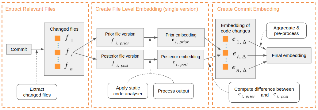
Embedding Pipeline

Figure 1. Embedding Pipeline

4.1. RQ1 Study Design

We extracted the embeddings for all commits in the dataset, as depicted in Figure 1. We analyzed the files contained in the commits of our dataset and their precessors using the static code analyzers introduced in Section 2. The three main phases of the pipeline are (i) extracting the relevant source code files, (ii) creating a numerical representation of these files, and (iii) aggregating them into an embedding for the whole commit. We computed one embedding per tool and applied several pre-processing steps to obtain the final embeddings. Finally, we computed several statistical tests that allowed us to answer RQ1.

4.1.1. Extracting Relevant Source Code Files

First, we identify which files of the repository were changed throughout the commit. We collect the version before the commit (prior version) and the version after the commit (posterior version) for each of these files. For performance reasons, we only select files that are affected by a vulnerability in the commit. Since we are interested in capturing code changes, files without any change are not relevant to us.

4.1.2. Creating File Level Embeddings

Second, we create embeddings for each of the collected files. We apply a static code analyzer to each of the relevant files. Next, we create an embedding for the files by transforming the tool’s output into a numerical representation. The specific transformation steps depend on the type of tool and will be explained in the following. If a file is created or added, all measures for the previous/current version are set to zero.

Static Code Analyzed based on Pattern Matching

We use two different bug finders, PMD and Checkstyle, to create embeddings that quantify bug changes between versions. Both tools return the list of bugs and the lines where they occur. Based on this, we calculate how often each bug occurs in the file. The result is a single version embedding with one column per bug and one line per changed file and version. Each value indicates how often a certain bug occurs in the file for a specific version. Some bug descriptions in the output generated by PMD include information like variable names. These bugs are renamed to more general names without such case-specific information to compare them across different files and repositories. For PMD, we apply all rules from all categories available. For Checkstyle, we used two example configuration files provided by the tool.

Static Code Analyzed based on Software Metrics

CK returns four CSV files: class.csv, field.csv, method.csv, and variable.csv. We only use the class.csv file since it captures the software metrics at the file level. Each line of this file represents one class in the repository and contains the information concerning which file the class is located in, the class type, different software metrics.

Static Code Analyzed based on Program Analysis

To create this embedding, first, we extracted the graphs from the source code files using Progex. Then, we measure their characteristics using several metrics. We limit the analysis to ASTs and CFGs and analyze these graphs using Networkx, a popular Python package for the network analysis. Some measures can be computed if only some condition is fulfilled. In case these conditions are met, the score is set to zero for that instance. For example, assortativity measures can be computed for graphs that contain at least one edge since the similarity of connections can be computed if such connections exist in the first place. Distance measures are meaningful only for connected graphs such as ASTs. The number of components is informative only for disconnected graphs such as CFGs because ASTs are always connected.

4.1.3. Computing Commit Embeddings

We compute the file-level embedding of the commit. For each file, we compute the difference between the measures in the previous and the current version. Next, the file-level numerical representation is aggregated at the commit level. We add two features indicating a positive or negative change for each feature at the file-level embedding: the first to aggregate positive file-level changes and the second to aggregate negative file-level changes. This step allows us to avoid information loss: a simple sum over all the feature values could have balanced positive and negative values. Finally, we drop all duplicate columns and columns with constant values.

4.1.4. Evaluating Embedding based on Static Analyzer to distinguish Security-relevant Commits

We use the Chi-square independence test to assess to what extent static code analyzer can be employed to create embeddings to distinguish security relevant commits (i.e., RQ1). For each feature, the null hypotheses is that the feature is independent (i.e., does not impact) on the security relevance of a commit. We choose Chi-square since it is a non-parametric test and, therefore, it is robust to data distributions (McHugh, 2013). Although most statistical tests assume a random sample, this technique is commonly applied for convenience samples. Chi-square is designed for two variables belonging to mutually exclusive categories like in our case. Based on these variables, a contingency table is created. The smallest number in any of the contingency table cells should be no less than five (McHugh, 2013). To comply with this requirement, if more than 90% of all values for a feature are zero, we convert this feature into a binary variable. Otherwise, we create one class for all not modified instances and bin the remaining values into $k$ different categories, indicating the strength of the change in the variable. We select $k$ as the highest number of possible equally-sized bins per feature to avoid splitting the same values over multiple bins. In particular, we distributed the values of the features resulting from the PMD and Progex over four bins; we composed seven bins for each feature resulting from CK and five bins for each feature resulting from Checkstyle. The remaining assumptions are the following: (i) the data in the cells of the contingency table should be counts, (ii) each subject (in our case: each commit) should only fall into one cell of the table, and (iii) the classes should be independent. For contingency tables with one degree of freedom, we used the recommended Yates’ correction of continuity (Cochran, 1952). Since Chi-square is a test of significance but not strength, we use Cramer’s V when Chi-square rejects the null hypothesis (McHugh, 2013). Results below $0.1$ represent no association, between $0.1$ and $0.3$ low association, between $0.3$ and $0.5$ moderate association, and above $0.5$ high association. We implement Chi-square and Cramer’s tests in Python using the scipy library. We use Yates’ correction and interpret it with $\alpha=0.05$.

4.2. RQ1 Results

We applied two statistical tests to evaluate whether there is a significant difference between security-relevant and non-security-relevant commits for the individual columns of the embeddings. First, we applied Chi-square; then, we evaluated the strength of the association using Cramer’s V.

Chi-Square Test

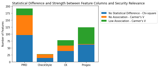
Features with significant code changes and their strength between security-relevant and non-security-relevant commits per embedding.

Figure 2. Features with significant code changes and their strength between security-relevant and non-security-relevant commits per embedding.

As depicted in Figure 2, the embeddings based on PMD and Progex have the highest number of features which show significant differences between security-relevant and non-security-relevant commits with 96 and 62 features, respectively. If these features represent 84% of features resulting from Progex, they represent only 21% of features for PMD. 45% of all features in CK show significant differences between classes, while only 11% of features (i.e., 14 out of 122) resulting from Checkstyle significantly capture differences.

Cramer’s V

For the features that showed a significant association with the target variable, we computed Cramer’s V to assess the strength of this association. Figure 2 shows the results for this test. All features of the four embeddings have a low association or no association at all. Almost all features of the Progex embedding, which showed significant differences between classes, had a low association between the target variable and the respective column. For Checkstyle, on the other hand, all columns except one showed no association in terms of Cramer’s V.

Summary of RQ1. Taken alone, most of the features resulting from the static analysis tools are not significantly different for security-relevant and non-security-relevant commits. If differences are significant, the association strength is low.

5. Levaraging on Static Code Analyzers Embeddings to Detect Security-relevant Commits

In this section, we answer the second research question which aims at understanding to what extent the embeddings resulting from static code analyzers can be used to train machine learning models to classify security-relevant commits.

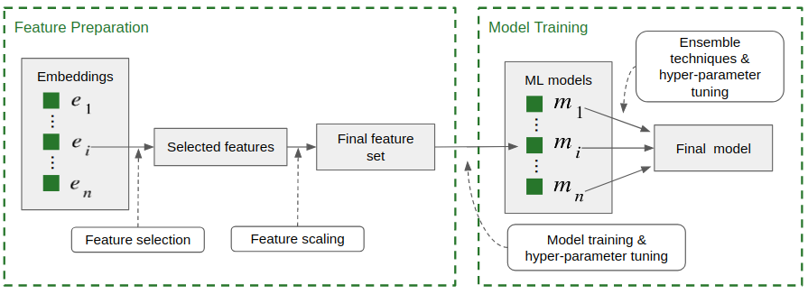
Machine Learning Pipeline

Figure 3. Machine Learning Pipeline

5.1. RQ2 Study Design

We trained multiple prediction models to identify security-relevant commits using the embeddings created in the previous section. Figure 3 depicts an overview of the adopted machine learning pipeline. First, we train models separately for each of the four embeddings. The embeddings are pre-processed using feature selection and feature scaling. We train a model per embedding using seven different machine learning algorithms and tune the hyperparameter values of the feature pre-processing and model training steps through a randomized search.

Dependent Variable

The variable to be predicted is the security relevance of a commit, where one indicates that a commit fixes a vulnerability and zero that it does not. The prediction problem is a binary classification problem.

Independent Variables

The independent features are the previously described embeddings, computed using the four static analysis tools. In the first step, the embeddings are used separately (i.e., one model per embedding). Then, these models are combined using voting and stacking techniques.

Evaluation Metrics

Performance metrics of binary classification problems are inherently tied to the number of correct and incorrect predictions for both classes, which are often visualized in a confusion matrix. The focus of this research is precision, which is interpreted along with recall using precision-recall curves. PR curves are a useful alternative to ROC curves to highlight the performance differences that are lost in ROC curves (Boyd et al., 2013). Furthermore, we also calculate accuracy and F1 scores (Baeza-Yates et al., 1999) to capture the general performance of our models.

Model Validation

Each model is trained and tuned using stratified k-fold cross-validation with $k=5$. $k$-fold cross-validation randomly splits the dataset into $k$ mutually exclusive subsets of equal size. The predictor is then trained $k$ times, each time using one fold for testing and the remaining $k-1$ folds for training. In stratified cross-validation, the folds contain approximately the same proportion of labels as the original dataset (Kohavi et al., 1995). We use the same folds used in commit2vec (Cabrera Lozoya et al., 2021) leveraging on the ”test_fold” variable in the dataset that indicates the fold to which each commit belongs.

5.1.1. Feature Selection

Feature selection helps to reduce computation time, improve prediction performance, and give a better understanding of the data by removing correlated variables, which do not provide extra information about the classes and thus serve as noise for the predictor. We apply three different types of feature selection techniques. First, we remove features whose variance falls below the chosen threshold (Li et al., 2017). This step is especially relevant for the static analyzers based on pattern matching, which are very sparse. Features with low variance contain little information and can, therefore, not discriminate between classes. Since a feature’s variance depends on the scale, we applied a min-max scaler before calculating the features’ variances. We only use scaled features only for the selection: the final feature set consists of the unscaled version of these features. Second, we apply the Pearson correlation coefficient (Pearson, 1895). Third, we perform recursive feature elimination Guyon et al. (Guyon et al., 2002). This technique is an example of backward feature elimination, starting with the full set of features and removing features iteratively. Each iteration consists of three steps: (i) train the classifier, (ii) compute the ranking criterion for all (remaining) features, (iii) remove the feature (or the set of features) with the smallest ranking criterion. We implement RFE using scikit-learn . We use these techniques independently and together, applying random search to find the best combination of techniques and the best hyperparameters. The parameter grid for feature selection can be found in the online appendix.

5.1.2. Feature Scaling

To prepare the predictive variables for model training, we apply scikit-learn’s StandardScaler, which scales and centers features by subtracting the mean and dividing by the standard deviation. We scale the feature set since some machine learning techniques can be negatively impacted by data distribution and scale differences between features.

5.1.3. Base Machine Learning Classifiers

First, we train multiple different models for each of the four embeddings. Specifically, we use seven different algorithms for model training: Decision Trees, Random Forests, AdaBoost, Gradient Boosting, Support Vector Machines, Logistic Regression, and Gaussian Naïve Bayes. These classifiers belong to different families and complement each other in terms of pros and cons, mixing some of the simplest techniques (i.e., Gaussian Naïve Bayes and Logistic Regression), with more complex ones (i.e., Random Forests, AdaBoost, and Gradient Boosting). All of the above techniques were implemented using scikit-learn, a well-known Python framework.

Hyperparameter Tuning

For each embedding, we train the models using the machine learning techniques described before. We evaluate the effect of feature selection by training each model once with and without feature selection. Please consider that we could not apply Recursive Feature Elimination to Gaussian Naïve Bayes and Support Vector Machines since they do not provide feature importances. A random search over the hyperparameter space is applied using scikit-learn’s RandomizedSearchCV. This algorithm randomly samples the hyperparameter from the distributions specified as part of the online appendix, those not specified are kept to their default values provided by scikit-learn. We run the randomized search for 200 iterations per machine learning technique, embedding, and combination of feature pre-processings steps. We selected this method instead of a more refined (i.e., GridSearch) because the base models are optimized on many hyper-parameters. Some are tuned along with numerical scales leading to the high-dimensional optimization problem.

5.1.4. Ensemble Techniques

In a second step, the models trained on the separate embeddings are combined through ensemble techniques, which combine multiple different classifiers to make a final prediction. We select the best performing model for each embedding regarding feature selection, machine learning algorithm, and hyper-parameter values. We use Voting and Stacking to combine these base models. Voting (Kittler et al., 1998) combines several estimators either by taking a majority vote or by averaging the predicted probabilities of the base estimators to make a final prediction. We use the VotingClassifier provided by scikit-learn. In particular, we use the soft vote option, which refers to the second case of averaging the predicted probabilities. Stacking (Wolpert, 1992) stacks the predictions of the individual estimators together and uses them as input to a final estimator to compute the prediction. The final estimator is trained through cross-validation. We use the StackingClassifier provided by scikit-learn.

Hyperparameter Tuning

The hyper-parameter settings of the final classifiers are optimized for precision using GridSearchCV on the same five-folds as in the base models’ case. We adopted this technique because of the smaller number of hyperparameters. Therefore, we want to test all possible combinations in the hyperparameter space. The parameter grid for each ensemble technique can be found in the online appendix. The hyperparameters, which are not featured in the tables, were left at their default values. We set up the weights of the base models for Voting to either fully include or exclude each base model in the prediction. This step allows examining which models complement each other and, following, which combination of models results in the best predictions. When using Stacking, we employed all previously described base models as final estimators.

We analyze the performance of the machine learning models, which were trained on the embeddings. We discuss the quality of the models trained first with base classifiers and then applying stacking and voting. We compare the results for these two different ensemble techniques and discuss whether the ensemble models reach higher predictive performance than the base models. Finally, we compare our best model and commit2vec in terms of predictive performance and training time and discuss the extent to which the two approaches are complementary.

5.2. RQ2 Results

We provide the results for the base machine learning classifiers, the ensemble techniques, and the comparison with commit2vec.

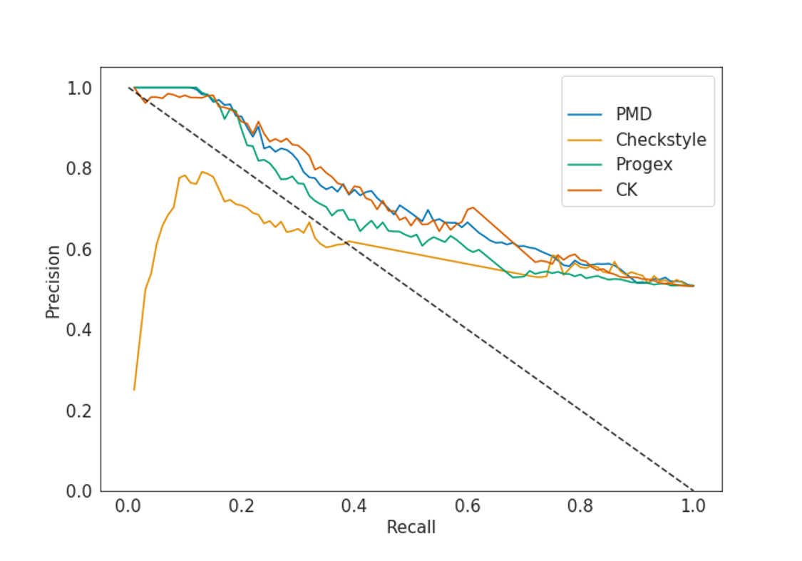
Precision-recall curves of the best model per embedding. The curves have been averaged over the five folds.

Figure 4. Precision-recall curves of the best model per embedding. The curves have been averaged over the five folds.

Table 1. The evaluation metrics of the best performing model per embedding. The table displays the mean and standard deviations of the metrics for each embedding.

Embedding	Precision	Recall	F1-Score	Accuracy
CK	75.62 $\pm$ 5.60	40.07 $\pm$ 1.28	52.34 $\pm$ 2.11	63.05 $\pm$ 2.50
Checkstyle	64.89 $\pm$ 3.69	31.25 $\pm$ 3.36	42.05 $\pm$ 2.78	56.56 $\pm$ 1.44
PMD	75.44 $\pm$ 5.37	35.50 $\pm$ 4.01	48.05 $\pm$ 3.30	61.35 $\pm$ 1.58
Progex	69.27 $\pm$ 4.01	38.25 $\pm$ 4.14	49.23 $\pm$ 4.22	60.18 $\pm$ 3.15

5.2.1. Base Machine Learning Classifiers

Figure 4 presents the precision-recall curves for the best performing model of each embedding. As can be seen, the models based on PMD and CK perform the best. The model trained on the Progex embedding reached a good but lower performance. Although the CK model is close to the other models’ performance for thresholds with high recall and low precision, it does not perform well when the target is high precision.

Table 1 show the performance of the best models for each embedding in terms of precision, recall, accuracy, and F1 score when optimizing the prediction threshold for precision. For the specific thresholds chosen, the CK model performs the best regarding all four evaluation metrics. Similarly, the Checkstyle model reaches the worst performance for all four metrics. The PMD model performs better than the Progex model regarding precision and accuracy but performs worse in terms of recall and F1 score.

Analyzing the best models in details, we can note that the models based on PMD and CK adopt Random Forest, while those leveraging the features extracted from CheckStyle and Progex use Gradient Boosting. For the sake of space, we report the configuration of these models in our online appendix.

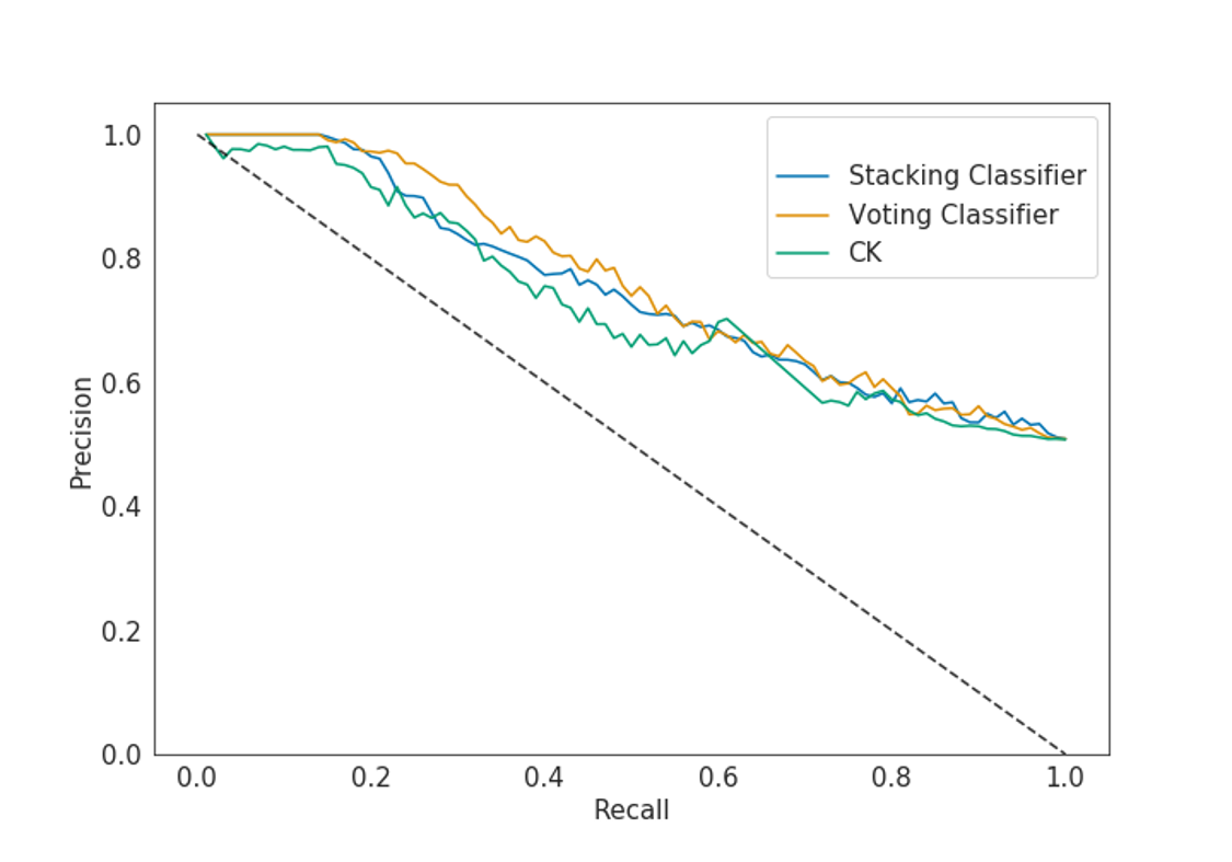
Precision-recall curves of the best model per ensemble. The curves have been averaged over the five folds.

Figure 5. Precision-recall curves of the best model per ensemble. The curves have been averaged over the five folds.

Table 2. The evaluation metrics of the best performing model per ensemble technique. The table displays the mean and standard deviations of the metrics for each ensemble technique.

Embedding	Precision	Recall	F1-Score	Accuracy
Stacking	74.75 $\pm$ 4.87	45.89 $\pm$ 5.02	56.56 $\pm$ 2.94	64.52 $\pm$ 1.60
Voting	77.51 $\pm$ 5.28	48.64 $\pm$ 1.71	59.68 $\pm$ 1.55	66.73 $\pm$ 2.13

5.2.2. Ensemble Techniques

We combined the four models from the previous section using the two different ensemble techniques: stacking and voting. Figure 5 shows the precision-recall curve for both the final models. It can be seen that for thresholds with high recall and lower precision, the two models perform very similarly. For our aim of maximizing precision, however, the voting classifier performs better. We then optimized the prediction thresholds of both models in terms of precision. Table 2 show the values of the evaluation metrics for the chosen thresholds. The voting classifier performs better than the stacking classifier in terms of all four metrics and achieves an average precision of 77.5% and an average recall of 48.64%.

We compared the precision-recall curves of the voting classifier to those of the models based on the individual embeddings. Combining the models leads to significantly better results, indicating that the models are complementary to each other.

5.2.3. Comparison with commit2vec

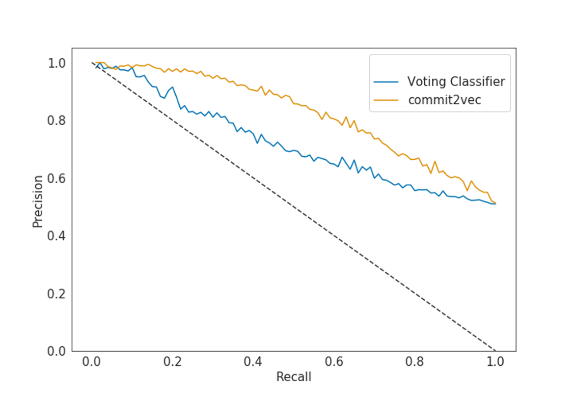
Precision-recall curves of commit2vec and voting classifier on the commits analyzable by commit2vec. The curves have been averaged over the five folds.

Figure 6. Precision-recall curves of commit2vec and voting classifier on the commits analyzable by commit2vec (i.e., $\approx 20\%$ of commits in our dataset). The curves have been averaged over the five folds.

Applying Commit2vec imposes several technical constraints, mostly stemming from implementation limitations, some of which inherited from code2vec (on which commit2vec is based). In particular, code2vec represents methods, and based on this represention, Commit2vec represents commits in terms of method changes. As a consequence, that commits that do not change methods cannot be processed. Furthermore, when analyzing method changes, commit2vec works under the condition that the name of methods is not altered by a commit, which of course is not always the case.

Therefore, commit2vec could process only around 20% of the commits in our dataset. However, as shown in Figure 6, commit2vec performs better than our models on the commits that it could process. For prediction thresholds resulting in high precision and lower recall, the performance of the two models is very similar. However, for thresholds with lower precision, commit2vec performs better.

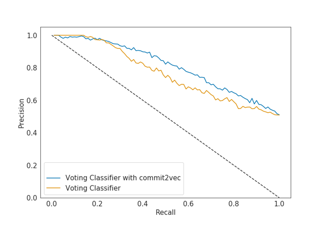
Precision-recall curves of the voting classifier and the combination of the voting classifier and commit2vec. The curves have been averaged over the five folds.

Figure 7. Precision-recall curves of the voting classifier and the combination of the voting classifier and commit2vec. The curves have been averaged over the five folds.

In practice, our method and commit2vec turn out to be complementary: one could use commit2vec when possible, and fall-back to our models in the other cases. Figure 7 visualizes the precision-recall curves of the voting classifier and the model obtained in the previously described way. Combining the two models, we can achieve much better performance than using any of them independently.

An in-depth comparison of the training times for commit2vec and our approach is out of the scope of this research. However, please note that our approach is likely to be much faster. Complex deep learning approaches like commit2vec are typically computationally very expensive. Code2vec, on which commit2vec is based, takes 1.5 days on a single Tesla K80 GPU to thoroughly train a model (Alon et al., 2019). In comparison, our approach takes less than half a day on an ordinary laptop, giving a strong indication that our approach is much less computationally expensive than commit2vec.

Summary of RQ2. Machine learning models constructed from features obtained from static analysis tools yield a slighly lower prediction performance than commit2vec. However, they can work with commits that commit2vec is not capable of representing. Ultimately, the two approaches complement each other and are best used in combination.

6. Threats to Validity

This section describes the threats to validity of our study.

Construct Validity

This research is inherently based on the definition of software vulnerabilities and commits that are likely to fix such vulnerabilities. The classification of commits in our dataset into security-relevant and non-security-relevant commits is not based on a formal definition. The dataset was created based on practical considerations, and vulnerabilities are only implicitly defined through their fix-commits. Therefore, our data could not fully represent vulnerabilities and their fix-commits.

Internal Validity

The results of our study are tied to the specific static code analyzers and pre-processing steps of their outputs, which we used to create the embeddings. Other static code analyzers or other pre-processing approaches may significantly change the results. We mitigated this risk through researching, which static code analyzers and pre-processing steps have been applied in related software engineering prediction tasks and following a similar research design.

External Validity

The dataset we used contains repositories, which are practical relevant to SAP, the company which provided the dataset. Within these repositories, there might be a bias towards easily reachable commits. Since part of the dataset was manually curated, certain types of commits might have been harder to reach and not represented appropriately in the dataset. Furthermore, our data distribution might not reflect the actual distribution of vulnerability types. Due to the reasons above, the generalizability of our findings to other industrial or academic settings might be limited.

Conclusion Validity

The data, which we used for the statistical test to address RQ2 does not fully comply with the assumptions of the chi-square test. First, the data was not obtained through random sampling. Second, not all cells in the contingency table initially had values of five or higher, which might affect the results of the test. We mitigated this risk by binning the initial data into several categories to ensure that all cells in the contingency table have values of at least five. The metrics used to evaluate our defect prediction approach (i.e., precision, recall, F-Measure, and accuracy) are widely used in the evaluation of the performances of defect prediction techniques (Boyd et al., 2013; Baeza-Yates et al., 1999). We used the precision-recall curves, an alternative and more conservative visualization than ROC curves, to evaluate the models’ overall performance.

7. Related Work

This section provides a comprehensive overview of the previous work related to vulnerability prediction and methods levering on features resulting from static analysis tools.

7.1. Vulnerability Prediction

Several surveys exist on the mitigation of software vulnerabilities. Shahriar and Zulkernine (Shahriar and Zulkernine, 2012) present and categorize work on the topic, published between 1994 and 2010. They found that most approaches fall into the following three categories: dynamic analysis, static analysis, and hybrid analysis. A later survey by Ghaffarian and Shahriari (Ghaffarian and Shahriari, 2017) covers the work between 2000 and 2016 and focuses on the application of machine learning and data mining approaches to analyze software vulnerabilities. Common approaches include vulnerability prediction models based on software metrics, anomaly detection approaches, and vulnerable code pattern recognition. The performance of vulnerability analysis models is typically analyzed in terms of false positives and false negatives. Both reviews report that no solution that is satisfactory on both dimensions has been found so far. In practice, the main challenge remains the false positive rate, as it requires large amounts of manual labor to identify vulnerable code instances among an extensive set of positive predictions. Existing research deviates from this work in multiple ways; the most crucial difference is the unit of analysis. In this work, we are not interested in identifying if a software component is vulnerable but instead if a commit is likely to fix a vulnerability. Furthermore, the focus of most existing approaches is a method or file-level analysis. We instead use whole repositories as our unit for analysis.

The closest work to ours is commit2vec (Cabrera Lozoya et al., 2021). Commit2vec represents whole commits on a repository level to identify security-relevant commits. The model is based on code2vec (Alon et al., 2019), which creates continuous embeddings for code snippets relying on abstract syntax trees and neural networks. Because of the former, Commit2vec can detect vulnerability only on compilable classes. Our approach does not exhibit this limitation, as we are using a broader set of features to build our models, which is not restricted to features extracted from the AST. Next to program analysis-related features, we also create features based on pattern matching and software metrics.

Nguyen and Tran (Nguyen and Tran, 2010) compute code metrics based on dependency graphs, obtained by static code analyzers, to predict vulnerable software components. This study computed a set of metrics on the dependency graph of software systems and used them as input for machine learning models. The empirical results were promising and suggested the effectiveness of using dependency graphs for detecting software vulnerabilities. Our work focus on a different unit of analysis, focusing on code changes instead of single versions. Furthermore, our work examines the usefulness of a broader range of static code analyzers for vulnerability prediction.

7.2. On the Use of Static Code Analysers in Software Engineering Prediction Tasks

Static code analyzers have been used to create different feature sets for prediction tasks in software engineering: software metrics, graph-based metrics, and patter-matching-based metrics.

7.2.1. Pattern-Matching Metrics

Lujan et al. (Lujan et al., 2020) recently used the output of bug finders to predict code smells, namely poor implementation choices applied during software evolution that can affect source code maintainability (Fowler, 2018). As more attention has been dedicated to machine learning solutions for identifying code smells (Di Nucci et al., 2018), the authors examine the role of static analysis warnings as features of machine learning models for detecting code smell types. Specifically, Checkstyle, FindBugs, and PMD are used to detect three types of code smells. Based on the output of such tools, a feature set was constructed by providing the number of violations exhibited by the software components for each warning. The evaluation results show that the warning types that contribute the most to the performance of the models depend on the considered code smell. Furthermore, the performance of the models built using the warnings of static analysis tools can drastically improve the capabilities of alternative code smell prediction models.

7.2.2. Software Metrics

Software metrics have also been used as a feature set for a variety of other prediction tasks. Most notably, they have been used in software fault and technical debt prediction.

Software fault prediction aims to detect faulty constructs such as modules or classes in the early phases of the software development life cycle (Malhotra, 2015; Li et al., 2018). Malhotra (Malhotra, 2015) reports that most studies use software metrics as independent variables for the prediction task. The mainly usedsoftware metrics are procedural, object-oriented, or hybrid metrics. CK metrics, defined by by Chidamber and Kemerer (Chidamber and Kemerer, 1994), are the most commonly used software metrics, out of which multiple metrics were found helpful for software fault prediction. The survey results indicate that machine learning techniques perform better than traditional statistical models for software fault prediction. Li et al. (Li et al., 2018) divide software metrics into code and process metrics. Code metrics represent the source code complexity, while process metrics represent the development process complexity. They also found that the CK metrics are among the most representative metrics for object-oriented programs.

Technical debt refers to design decisions that allow software development teams to achieve short-term benefits such as timely code releases. Technical debt needs to be managed carefully to avoid severe consequences in the future. The technical debt items are usually documented, including the required effort to resolve the item. Then, the items are prioritized and addressed accordingly. Codabux and Williams (Codabux and Williams, 2016) propose a framework to prioritize technical debt items using data mining and machine learning models. The authors extract class-level software metrics for defect- and change-prone classes. Then, a prediction model is built based on these metrics to determine the technical debt proneness of each class. The predictions are finally used to categorize the items according to their debt proneness probability.

7.2.3. Graph-Based Metrics

Several papers use dependency graphs to identify program units that are more likely to face defects. Zimmermann and Nagappan (Zimmermann and Nagappan, 2008) propose using network analysis on the dependency graphs to train regression models to predict defects. The results were deemed promising as the graph-based models performed significantly better than the code metrics-based models. Two replication studies were conducted to test the generality of the findings with contrasting results (Premraj and Herzig, 2011; Tosun et al., 2009). Bhattacharya et al. (Bhattacharya et al., 2012) considered a broader scope by using network metrics for bug severity estimation and refactoring efforts prioritization, next to the prediction of defects. Their approach is based on graphs at different levels of granularity. The evaluation of this approach, conducted on multiple programs, indicates that graph metrics can predict bug severity, maintenance effort, and defect-prone releases.

8. Conclusion and Future Work

In recent years, the need for automated identification of security-relevant commits emerged to ensure software security. We address this need by proposing a framework to use static code analyzers combined with machine learning techniques to detect security-relevant commits. We created four different embeddings based on off-the-shelf code analyzers (PMD, Checkstyle, CK, and Progex). We statistically evaluated whether the features of the embeddings differ significantly for security-relevant and non-security-relevant commits. Then, we created machine learning models based on the embeddings to predict the security relevance of commits. Our results indicate no significant difference in the embeddings between security-relevant and non-security-relevant commits when looking at the features individually. However, we show that successful machine learning models based on base classifiers and ensemble techniques can be trained on the combination of the features. Compared to commit2vec, our model has a slightly lower predictive performance, but it can predict a broader range of commits. Finally, a model integrating both approaches achieves better results than those obtained by the approaches independently.

As future work, we aim to extend our empirical study on a different dataset with industrial and academic settings. We also plan to experiment with other code analyzers and different ways of processing their output. Since data about security-relevant commits is scarce, we believe that transfer learning can be a valuable direction to explore, similarly to the work of Cabrera Lozoya et al. (Cabrera Lozoya et al., 2021). Finally, embeddings based on static code analyzers could be used for other prediction tasks on source code such as automatic code repair and defect prediction.

- (1)
- Alon et al. (2019) Uri Alon, Meital Zilberstein, Omer Levy, and Eran Yahav. 2019. Code2vec: Learning Distributed Representations of Code. Proc. ACM Program. Lang. 3, POPL, Article 40 (Jan. 2019), 29 pages. https://doi.org/10.1145/3290353
- Baeza-Yates et al. (1999) Ricardo Baeza-Yates, Berthier Ribeiro-Neto, et al. 1999. Modern information retrieval. Vol. 463. ACM press New York.
- Bhattacharya et al. (2012) Pamela Bhattacharya, Marios Iliofotou, Iulian Neamtiu, and Michalis Faloutsos. 2012. Graph-based analysis and prediction for software evolution. In 2012 34th International Conference on Software Engineering (ICSE). IEEE, 419–429.
- Boyd et al. (2013) Kendrick Boyd, Kevin H Eng, and C David Page. 2013. Area under the precision-recall curve: point estimates and confidence intervals. In Joint European conference on machine learning and knowledge discovery in databases. Springer, 451–466.
- Cabrera Lozoya et al. (2021) Rocío Cabrera Lozoya, Arnaud Baumann, Antonino Sabetta, and Michele Bezzi. 2021. Commit2Vec: Learning Distributed Representations of Code Changes. SN Computer Science 2, 3 (19 Mar 2021), 150. https://doi.org/10.1007/s42979-021-00566-z
- Chidamber and Kemerer (1994) Shyam R Chidamber and Chris F Kemerer. 1994. A metrics suite for object oriented design. IEEE Transactions on software engineering 20, 6 (1994), 476–493.
- Cochran (1952) William G Cochran. 1952. The 2 test of goodness of fit. The Annals of mathematical statistics 23, 3 (1952), 315–345.
- Codabux and Williams (2016) Zadia Codabux and Byron J Williams. 2016. Technical debt prioritization using predictive analytics. In 2016 IEEE/ACM 38th International Conference on Software Engineering Companion (ICSE-C). IEEE, 704–706.
- Di Nucci et al. (2017) Dario Di Nucci, Fabio Palomba, Giuseppe De Rosa, Gabriele Bavota, Rocco Oliveto, and Andrea De Lucia. 2017. A developer centered bug prediction model. IEEE Transactions on Software Engineering 44, 1 (2017), 5–24.
- Di Nucci et al. (2018) Dario Di Nucci, Fabio Palomba, Damian A Tamburri, Alexander Serebrenik, and Andrea De Lucia. 2018. Detecting code smells using machine learning techniques: are we there yet?. In 2018 ieee 25th international conference on software analysis, evolution and reengineering (saner). IEEE, 612–621.
- Fowler (2018) Martin Fowler. 2018. Refactoring: improving the design of existing code. Addison-Wesley Professional.
- Frei et al. (2010) Stefan Frei, Dominik Schatzmann, Bernhard Plattner, and Brian Trammell. 2010. Modeling the security ecosystem-the dynamics of (in) security. In Economics of Information Security and Privacy. Springer, 79–106.
- Ghaffarian and Shahriari (2017) Seyed Mohammad Ghaffarian and Hamid Reza Shahriari. 2017. Software Vulnerability Analysis and Discovery Using Machine-Learning and Data-Mining Techniques: A Survey. ACM Comput. Surv. 50, 4, Article 56 (Aug. 2017), 36 pages. https://doi.org/10.1145/3092566
- Guyon et al. (2002) Isabelle Guyon, Jason Weston, Stephen Barnhill, and Vladimir Vapnik. 2002. Gene selection for cancer classification using support vector machines. Machine learning 46, 1-3 (2002), 389–422.
- Kittler et al. (1998) Josef Kittler, Mohamad Hatef, Robert PW Duin, and Jiri Matas. 1998. On combining classifiers. IEEE transactions on pattern analysis and machine intelligence 20, 3 (1998), 226–239.
- Kohavi et al. (1995) Ron Kohavi et al. 1995. A study of cross-validation and bootstrap for accuracy estimation and model selection. In Ijcai, Vol. 14, no. 2. 1137–1145.
- Li et al. (2017) Jundong Li, Kewei Cheng, Suhang Wang, Fred Morstatter, Robert P. Trevino, Jiliang Tang, and Huan Liu. 2017. Feature Selection: A Data Perspective. ACM Comput. Surv. 50, 6, Article 94 (Dec. 2017), 45 pages. https://doi.org/10.1145/3136625
- Li et al. (2018) Zhiqiang Li, Xiao-Yuan Jing, and Xiaoke Zhu. 2018. Progress on approaches to software defect prediction. IET Software 12, 3 (2018), 161–175.
- Louridas (2006) Panagiotis Louridas. 2006. Static code analysis. Ieee Software 23, 4 (2006), 58–61.
- Lujan et al. (2020) Savanna Lujan, Fabiano Pecorelli, Fabio Palomba, Andrea De Lucia, and Valentina Lenarduzzi. 2020. A Preliminary Study on the Adequacy of Static Analysis Warnings with Respect to Code Smell Prediction. In Proceedings of the 4th ACM SIGSOFT International Workshop on Machine-Learning Techniques for Software-Quality Evaluation. Association for Computing Machinery, New York, NY, USA, 1–6. https://doi.org/10.1145/3416505.3423559
- Malhotra (2015) Ruchika Malhotra. 2015. A systematic review of machine learning techniques for software fault prediction. Applied Soft Computing 27 (2015), 504–518.
- McHugh (2013) Mary L McHugh. 2013. The chi-square test of independence. Biochemia medica: Biochemia medica 23, 2 (2013), 143–149.
- Nguyen and Tran (2010) Viet Hung Nguyen and Le Minh Sang Tran. 2010. Predicting Vulnerable Software Components with Dependency Graphs. In Proceedings of the 6th International Workshop on Security Measurements and Metrics (Bolzano, Italy) (MetriSec ’10). Association for Computing Machinery, New York, NY, USA, Article 3, 8 pages. https://doi.org/10.1145/1853919.1853923
- Pashchenko et al. (2021) Ivan Pashchenko, Riccardo Scandariato, Antonino Sabetta, and Fabio Massacci. 2021. Secure Software Development in the Era of Fluid Multi-party Open Software and Services. In 2021 IEEE/ACM 43rd International Conference on Software Engineering Companion (ICSE-C).
- Pearson (1895) Karl Pearson. 1895. VII. Note on regression and inheritance in the case of two parents. proceedings of the royal society of London 58, 347-352 (1895), 240–242.
- Ponta et al. (2020) Serena Elisa Ponta, Henrik Plate, and Antonino Sabetta. 2020. Detection, assessment and mitigation of vulnerabilities in open source dependencies. Empirical Software Engineering 25, 5 (01 Sep 2020), 3175–3215. https://doi.org/10.1007/s10664-020-09830-x
- Ponta et al. (2019) Serena Elisa Ponta, Henrik Plate, Antonino Sabetta, Michele Bezzi, and Cédric Dangremont. 2019. A manually-curated dataset of fixes to vulnerabilities of open-source software. In 2019 IEEE/ACM 16th International Conference on Mining Software Repositories (MSR). IEEE, 383–387.
- Premraj and Herzig (2011) Rahul Premraj and Kim Herzig. 2011. Network versus code metrics to predict defects: A replication study. In 2011 International Symposium on Empirical Software Engineering and Measurement. IEEE, 215–224.
- Sabetta and Bezzi (2018) Antonino Sabetta and Michele Bezzi. 2018. A Practical Approach to the Automatic Classification of Security-Relevant Commits. In 2018 IEEE International Conference on Software Maintenance and Evolution (ICSME). IEEE, 579–582.
- Schryen (2011) Guido Schryen. 2011. Is open source security a myth? Commun. ACM 54, 5 (May 2011), 130–140. https://doi.org/10.1145/1941487.1941516
- Shahriar and Zulkernine (2012) Hossain Shahriar and Mohammad Zulkernine. 2012. Mitigating program security vulnerabilities: Approaches and challenges. ACM Computing Surveys (CSUR) 44, 3 (2012), 1–46.
- Tal (2019) Liran Tal. 2019. The state of open source security report.
- Tosun et al. (2009) Ayşe Tosun, Burak Turhan, and Ayşe Bener. 2009. Validation of Network Measures as Indicators of Defective Modules in Software Systems. In Proceedings of the 5th International Conference on Predictor Models in Software Engineering (Vancouver, British Columbia, Canada) (PROMISE ’09). Association for Computing Machinery, New York, NY, USA, Article 5, 9 pages. https://doi.org/10.1145/1540438.1540446
- Wolpert (1992) David H Wolpert. 1992. Stacked generalization. Neural networks 5, 2 (1992), 241–259.
- Zaffar et al. (2011) Muhammad Adeel Zaffar, Ram L. Kumar, and Kexin Zhao. 2011. Diffusion dynamics of open source software: An agent-based computational economics (ACE) approach. Decis. Support Syst. 51, 3 (2011), 597–608. http://dblp.uni-trier.de/db/journals/dss/dss51.html#ZaffarKZ11
- Zimmermann and Nagappan (2008) Thomas Zimmermann and Nachiappan Nagappan. 2008. Predicting Defects Using Network Analysis on Dependency Graphs. In Proceedings of the 30th International Conference on Software Engineering (Leipzig, Germany) (ICSE ’08). Association for Computing Machinery, New York, NY, USA, 531–540. https://doi.org/10.1145/1368088.1368161