Adapting by Pruning: A Case Study on BERT

Abstract

Adapting pre-trained neural models to downstream tasks has become the standard practice for obtaining high-quality models. In this work, we propose a novel model adaptation paradigm, adapting by pruning, which prunes neural connections in the pre-trained model to optimise the performance on the target task; all remaining connections have their weights intact. We formulate adapting-by-pruning as an optimisation problem with a differentiable loss and propose an efficient algorithm to prune the model. We prove that the algorithm is near-optimal under standard assumptions and apply the algorithm to adapt BERT to some GLUE tasks. Results suggest that our method can prune up to 50% weights in BERT while yielding similar performance compared to the fine-tuned full model. We also compare our method with other state-of-the-art pruning methods and study the topological differences of their obtained sub-networks.

1 Introduction

From ResNet He et al. (2016) in computer vision to BERT Devlin et al. (2019) in NLP, large pre-trained networks have become the standard starting point for developing neural models to solve downstream tasks. The two predominant paradigms to adjust the pre-trained models to downstream tasks are feature extraction and fine-tuning Gordon et al. (2020). Both paradigms require adding some task-specific layers on top of the pre-trained model, but in feature extraction, the weights of the pre-trained model are “frozen” and only the task-specific layers are trainable, while in fine-tuning, weights in both the pre-trained model and the task-specific layers can be updated. Variants of these two paradigms include updating only selected layers in the original model Zhang et al. (2020), and the Adaptor approach which inserts trainable layers in between original layers Rebuffi et al. (2017); Houlsby et al. (2019). However, all these adaptation paradigms need to add new parameters and hence enlarge the model size. Consequently, running the adapted models, even at inference time, requires considerable resources and time, especially on mobile devices Ganesh et al. (2020); Blalock et al. (2020).

In this paper, we propose a novel model adaptation paradigm that we call adapt by pruning. Given a downstream task, we prune the task-irrelevant neural connections from the pre-trained model to optimise the performance; all remaining connections inherit the corresponding weights from the original pre-trained model. Our paradigm is inspired by the observation that large pre-trained models are highly over-parameterised Frankle and Carbin (2019) and pruning appropriate weights in large (randomly initialised) neural models can yield strong performance even without fine-tuning the weights Zhou et al. (2019); Wortsman et al. (2020). Our paradigm is particularly suitable for the applications on mobile devices Houlsby et al. (2019): the users only need to download the base model once, and as new tasks arrive, they only need to download a task-specific binary masks to adapt the base model to the new tasks. Table 1 compares our method with multiple model adaptation and compression paradigms. Fig. 1 provides a graphical explanation of our method.

	FullPerf	Eff	ReuseStruct	ReusePara
Feat.Ext.			✓	✓
FineTune	✓		✓
Adaptor	✓		✓	✓
Distillation	✓	✓
Pruning	✓	✓	✓
Ours	✓	✓	✓	✓

Table 1: Our method can achieve near full model performance (FullPerf) and has high inference-time efficiency (Eff), while reusing both the structure (ReuseStruct) and weights (ReusePara) of the original pre-trained model.

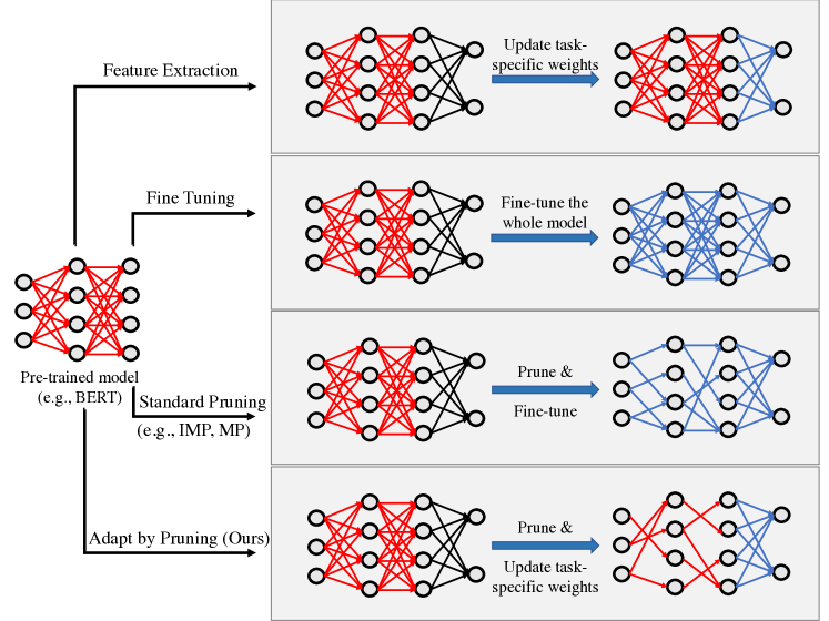
Figure 1: Comparison of different model adaptation paradigms. Red neural connections stand for the weights from the pre-trained model, blue for fine-tuned weights, and black for randomly initialised weights.

We exploit the idea that pruning can be formulated as learning how to mask the pre-trained model Colombo and Gao (2020). Let $f(x;w_{0},p)$ be the neural model for a downstream task, where $x$ is the input, $w_{0}\in\mathbb{R}^{d}$ are the weights of the pre-trained model, and $p\in\mathbb{R}^{k}$ the weights of all task-specific layers. Adapting $f$ by pruning amounts to finding the optimal binary mask $m^{*}\in\{0,1\}^{d}$, such that applying $m^{*}$ to $w_{0}$ maximises the performance of $f$ on the target task. The formal definition of the masking problem is provided in Eq. (3) in §3. This is a high-dimensional combinatorial optimisation problem, a highly challenging task in general.

Contributions

Firstly, we propose an efficient adapting-by-pruning algorithm (§3). We approximate mask searching as a differentiable optimisation problem, prove that, under standard assumptions, the error of the approximation is bounded, and propose an algorithm to efficiently find (near-)optimal masks. Our approach also allows the user to trade off between the performance and the efficiency of the pruned model by penalising the number of ones in $m^{*}$. The theoretical analysis and the proposed algorithm are general and, hence, define a generic model-adaptation paradigm.

Secondly, we test the effectiveness of our adapting-by-pruning algorithm by applying it to BERT Devlin et al. (2019) on multiple GLUE Wang et al. (2019) benchmark tasks. Results (in §4) suggest that our method can achieve the same performance as models adapted through feature-extraction but with (up to) 99.5% fewer parameters. Compared to fine-tuning, our method prunes up to 50% parameters in BERT while achieving comparable performance. We also show that, with the same number of parameters, sub-networks obtained by our method significantly outperforms those obtained by other state-of-the-art pruning techniques.

Finally, we inspect the differences between the masks obtained by ours and existing pruning methods, in particular the lottery ticket pruning methods Frankle and Carbin (2019); Chen et al. (2020). We find that the masks obtained by our method and lottery-ticket approaches have very different topological structures, but they also share some important characteristics, e.g., their performance is highly sensitive to mask-shuffling and weight-reinitialisation Frankle et al. (2020b). Furthermore, with ablation studies, we find that connection recovery, i.e., weights that are pruned in an early stage of the pruning process are reactivated in a later stage, is a key ingredient for the strong performance of our method, especially at high-sparsity levels. As connection recovery is not allowed in many popular pruning methods, this finding sheds light on the limitations of existing techniques. Our codes and the Supplementary Material can be found at https://github.com/yg211/bert_nli.

2 Related Work

Model Compression and Pruning.

Pruning is a widely used method to adapt pre-trained models to downstream tasks while reducing the model size. The lottery ticket hypothesis, which lays the foundation for many pruning works, states that a sub-network can be fine-tuned in place of the full model to reach comparable performance Frankle and Carbin (2019). The optimal sub-network is also known as the winning ticket. Recent experiments have confirmed the existence of winning ticket sub-networks in different pre-trained models, including BERT Frankle et al. (2020a).

Iterative magnitude pruning (IMP) Frankle and Carbin (2019) is the most widely used method for finding winning tickets. IMP involves three steps at each iteration: (i) training the network until convergence, (ii) removing a small percentage of connections (usually 10-20%) whose weights are closest to zero, and (iii) rewinding all remaining weights to their initial values. Such iterations are repeated until the target sparsity is reached. IMP is highly expensive because each iteration requires training the model to convergence and the obtained pruned network needs to be further fine-tuned. Cheaper alternative methods have been proposed Chen et al. (2020); Brix et al. (2020); Savarese et al. (2020), but the quality of their sub-networks are worse than IMP, and the obtained sub-networks also need to be fine-tuned. Compared to these pruning techniques, our method keeps all original weights intact, hence avoids the expensive fine-tuning step and allows for parameter reuse.

Other model compressing methods include weight quantization Shen et al. (2020); Fan et al. (2020), parameter sharing Lan et al. (2020) and attention layer decomposition Cao et al. (2020). Because our method reuses the original neural structure, these methods can be used together with our paradigm to further reduce the model size and the inference time.

Supermask & Neural Architecture Search.

Our work is inspired by works on supermasks such as Zhou et al. (2019). They find that applying appropriate binary masks to randomly initialised neural networks can improve the performance of the original model, even without updating the weights values. These binary masks are known as supermasks. Zhou et al. (2019) formulates the supermask learning problem as the problem of learning a Bernoulli distribution for each weight; at training time, they learn the distribution with standard stochastic gradient descent (SGD); in forward propagation, the activation status of each weight is sampled from the learnt distribution stochastically. However, in this case, users cannot explicitly control the sparsity of the pruned network.

Ramanujan et al. (2020) proposed an improved algorithm, edge-popup, which removes the stochasticity by ranking the importance of neural connections. Edge-popup provides better performance with smaller variance and allows users to specify the target sparsity. However, edge-popup was only tested on models with randomly initialised weights, and no proofs were provided regarding its optimality. Instead of learning a score to rank the neural connections, our method directly learns the $\{0,1\}$ values in the mask; this allows us to prove the optimality guarantees. Also, we apply our method to prune a pre-trained model (BERT) instead of the random-initialised models, and provide the first systematic comparison of the topological structures of supermasks and winning lottery tickets (in §4.2).

3 Our Method

Let $f(x;w_{0},p)$ denote the model for a downstream task, where $w_{0}$ are the weights from the pre-trained base model and $p$ the task-specific parameters. Our target is to find a task-specific optimal binary mask (supermask) for $w_{0}$. More formally, a supermask $m^{*}$ can be defined as

$$m^{*}={\arg\min}_{m\in\{0,1\}^{d}}\min_{p\in\mathbb{R}^{k}}\mathcal{L}(m,p),$$

$$\mathcal{L}(m,p)=|D_{train}|^{-1}\sum_{z\in D_{train}}\ell(z;m,p),$$ (1)

$$\ell(z;m,p)=\mathcal{G}\left(f(x;w_{0}\!\odot\!m,p),y\right),z=(x,y).$$

where $\odot$ is the element-wise product and $\mathcal{G}(\hat{y},y)$ a differentiable loss function, e.g., the least-squares or cross-entropy loss. Because $\mathcal{L}$ is differentiable with respect to its arguments, $p$ can be optimised with standard SGD techniques. However, as $m\in\{0,1\}^{d}$ is a discrete variable, we cannot directly use SGD approaches to optimise $\mathcal{L}$ with respect to $m$. In §3.1, we propose a continuous approximation of $\mathcal{L}$ and in §3.2 we prove that (near-)optimal supermasks can be obtained by optimising such a continuous approximation; in §3.3, we propose an algorithm to obtain supermasks of arbitrary sparsity.

3.1 Continuous Approximation

A natural method to approximate binary masks $m\in\{0,1\}^{d}$ is to use the sigmoid function, i.e., to replace $m$ with

$$m_{t}=\sigma(t\theta)=[1+\exp(-t\theta)]^{-1},\quad t>>1$$

where $\theta\in\mathbb{R}^{d}$ is a real-valued tensor of the same dimension as $m$, and $t$ is a hyper-parameter. With this approximation, the loss in Eq. (3) becomes a continuous function, i.e.,

$${\mathcal{L}}_{t}(\theta)=|D_{train}|^{-1}\!\!\!\sum_{z\in D_{train}}\!\!\!\ell(z;m_{t},p).$$ (2)

Since $m_{t}$ is differentiable with respect to $\theta$, the gradient of (2) is well defined as

$${\nabla}_{\theta} {\mathcal{L}}_{t}(\theta)=$$

$$|D_{train}|^{-1}\!\!\!\!\!\sum_{z\in D_{train}}\!\!\!\!\!\nabla_{m_{t}}\ell(z;m_{t},p)\odot\nabla_{\theta}m_{t}.$$ (3)

When $t\to\infty$, we have $m_{t}\to m$ and ${\mathcal{L}}_{t}\to{\mathcal{L}}$, i.e., the gap between the original objective function and its continuous approximation approaches zero. However, for any $\theta\neq 0$, $t\to\infty$ also implies $\nabla_{\theta}m_{t}=m_{t}\odot(1-m_{t})\to 0$ and hence the gradient in Eq. (3) also vanishes. To trade off between the quality of the approximation (Eq. (2)) and the magnitude of its gradient (Eq. (3)), we propose to use a larger $t$ in the forward propagation and a smaller $t$ in sigmoid gradient computation. More explicitly, we approximate Eq. (3) with

$$\tilde{\nabla}_{\theta}{\mathcal{L}}_{t}(\theta)=|D_{train}|^{-1}\!\!\!\!\!\sum_{z\in D_{train}}\!\!\!\!\!\tilde{\nabla}_{\theta}\ell(z;m_{t_{l}},m_{t_{s}},p)$$

$$\tilde{\nabla}_{\theta}\ell(z;m_{t_{l}},m_{t_{s}},p)=\nabla_{m_{t_{l}}}\ell(z;m_{t_{l}},p)\odot\nabla_{\theta}m_{t_{s}},$$ (4)

where $t_{l}$ and $t_{s}$ stand for the large and small values of $t$, respectively. The approximate SGD updates of $\theta$ and $p$ are

$$\theta_{i+1} :=\theta_{i}-\alpha_{i}\tilde{\nabla}_{\theta}\ell(z;m_{t_{l}},m_{t_{s}},p),$$ (5)

$$p_{i+1} :=p_{i}-\beta_{i}\nabla_{p}\ell(z;m,p),$$ (6)

where $\alpha_{i}$ and $\beta_{i}$ are learning steps, $\tilde{\nabla}_{\theta}\ell$ is defined in Eq. (3.1), $\nabla_{p}\ell$ is the exact gradient of $\ell$ (in Eq. (3)) with respect to $p$, and $z$ is chosen uniformly at random in $D_{train}$. After $T$ steps, a binary mask can be derived from $\theta_{T}$ by forcing all positive values in $\theta_{T}$ to be one and all negative values to be zero i.e., by letting $m_{T}\to\mathbbm{1}[\theta_{T}>0]$, where $\mathbbm{1}$ is the indicator function.

3.2 Convergence analysis

Let $v\in[0,1]^{d}$ denote an approximate mask, i.e., $v=\sigma(t\theta)$ for some $t>0$ and $\theta\in{\mathbb{R}}^{d}$. We assume that $\ell$ is convex in $v$ for all $z$, and that $\nabla_{v}\ell$ is bounded, i.e., that $\ell$ satisfies the assumption below.

Assumption 1.

For all $v,v^{\prime}\in[0,1]^{d}$, any possible input $z$ and any parameters $p\in\mathbb{R}^{k}$, $\ell(v,z)$ is differentiable with respect to $v$ and

$$\max_{z,v,p}\|\nabla_{v}\ell(z;v,p)\|^{2}\leq G^{2},$$

$$\ell(z;v,p)-\ell(z;v^{\prime},p)\geq\nabla_{v^{\prime}}\ell(z;v^{\prime},p)^{\intercal}(v-v^{\prime}),$$

where $G$ is a positive constant.

Under this assumption, we prove that the SGD steps in Eq. (5) produce a near-optimal mask.

Theorem 1.

Let $\ell$ meet Assumption 1 and $\{\theta_{i}\in{\mathbb{R}}^{d}\}_{i=1}^{T}$ be the sequences of stochastic weight updates defined in Eq. (5). For $i=1,\dots,T$, let $z_{i}$ be a sample drawn from $D_{train}$ uniformly at random, and $\alpha_{i}=\frac{c}{\sqrt{i}}$, where $c$ is a positive constant. Then

$$\mathbb{E}[{\cal L}_{t}(\theta_{T})- {\cal L}_{t}(\theta^{*})]\leq$$

$$\frac{1}{c\sqrt{T}}+\frac{cG^{2}(1+C)(1+\log T)}{T},$$

where the expectation is over the distribution generating the data, $\theta^{*}=\arg\min_{\theta\in\mathbb{R}^{d}}{\cal L}_{t_{l}}(\theta)$, $G$ is defined in Assumption 1 (with $v=\sigma(t_{l}\theta)$), and

$$C=t_{l}t_{s}\left(\frac{1}{t_{l}t_{s}}-2g_{max}(t_{l})g_{max}(t_{s})+\frac{t_{l}t_{s}}{16^{2}}\right)$$

$$g_{max}(t)=\sigma(tM)(1-\sigma(tM)),$$

with $M=\max\{|\theta_{i}|,i=1,\dots,T\}$.

Proof of Theorem 1 is provided in the Supplementary Material. Theorem 1 suggests that the expected gap between the loss evaluated at $\theta_{T}$ and the true minimum $\theta^{*}$ is bounded. For simplicity, we consider the convergence of Eq. (5) for fixed $p$, but a full convergence proof can be obtained by combining Theorem 1 with standard results for unconstrained SGD. By combining the Theorem 1 with $\lim_{t_{l}\to\infty}{\mathcal{L}}_{t_{l}}={\mathcal{L}}$, we conclude that a near-optimal supermask can be defined by

$$m^{*}=\lim_{t_{l}\to\infty}\sigma(t_{l}\theta_{T})=\mathbbm{1}[\theta_{T}>0].$$

3.3 Adapt by Pruning Algorithm

We can use SGD with Eq. (5) and (6) to obtain a near-optimal binary mask of undefined sparsity. Note that the number of zeros in the approximated mask $\sigma(t\theta_{T})$ is determined by the number of negative values in $\theta_{T}$. To encourage more negative values in $\theta$, we add a regularisation term in Eq. (5):

$$\theta_{i+1}:=\theta_{i}-\alpha_{i}\tilde{\nabla}_{\theta}\ell(z;m_{t_{l}},m_{t_{s}},p)-\gamma_{i}\mathbf{1},$$ (7)

where $\mathbf{1}$ is a tensor of the same dimension as $\theta$ and its elements are all $1$s, and $\gamma_{i}$ is the weight for the regularisation term. In practice, we can initialise $\theta$ with small positive values; the penalisation term will push the entries of $\theta$ to be negative, so that sparser masks can be obtained. To ensure that the target sparsity can be achieved with a similar number of epochs as regular training (i.e., one-shot pruning), the value of the hyper-parameter $\gamma_{i}$ should be tuned to control the pruning speed. Alg. 1 presents the pseudo code for the our supermask searching algorithm.

Algorithm 1 Adapt by Pruning Algorithm

Inputs: Pre-trained model $f(x;w_{0},\cdot)$, training data $D_{train}$, target sparsity $s$, hyper-parameters $t_{l}$ and $t_{s}$, initial parameters $\theta_{0}$ and $p_{0}$, learning steps $\alpha_{i},\beta_{i}$ and $\gamma_{i}$ for $i=1,\cdots,T$

Pruning:

  for $i=1,\cdots,T$ do

     Obtain $\theta_{i}$ following Eq. (7)

     Obtain $p_{i}$ following Eq. (6)

     break if ratio of negative values in $\theta_{i}$ is larger than $s$

  end for

Output: $p_{i}$ and the binary mask $m^{*}=\mathbbm{1}[\theta_{i}>0]$

4 Experiments

In this section, we test the efficiency of our pruning method by applying it to BERT-base. The BERT model and its weights are from the PyTorch implementation by HuggingFace. All our experiments are performed on a workstation with a single RTX2080 GPU card (8GB memory).

We consider three representative tasks from the GLUE benchmark Wang et al. (2019): STS-B (sentence similarity measurement), SST-2 (sentiment analysis), and MNLI (natural language inference). They cover a wide range of input types (single or pairwise sentences), output types (regression or classification), and data size; see Table 2 for their details. Since the official test set are not publicly available, we report the performance on their official Dev set.

	STS-B	SST-2	MNLI
Train	7k	67k	393k
Dev	1.5k	872	20k
Input	SentPair	SingleSent	Sentpair
Output	Score $\in[0,5]$	2-class label	3-class label
Metric	Spearman’s rho	Accuracy	Accuracy

Table 2: GLUE datasets used in the experiments.

For each task, we learn a weighted average of each layer’s [CLS] vector as the input to the task-specific MLP. The MLP has a ReLU hidden layer of the same dimension of the input (i.e., 768), followed by the output layer. Peters et al. (2019) have shown that using the weighted average of all layers outputs yields better performance than only using the last layer’s [CLS]. Parameters in the added MLP account for around 0.5% of the whole model size, and they are not pruned in our experiments, in line with other BERT pruning methods Chen et al. (2020); Brix et al. (2020).

Baselines

We compare our method with both feature extraction and fine-tuning, the two predominant paradigms of model adaptation. The performance of fine-tuning is widely regarded as the ‘upper-bound’ in model adaptation Houlsby et al. (2019) and model compression Ganesh et al. (2020). We also consider three pruning methods as baselines. Rnd is the random baseline: for a given sparsity level $s$, this method builds a mask such that each element is 0 with probability $s$ and 1 otherwise. IMP is the iterative magnitude pruning method (see §2); it is the most widely used heuristic for obtaining winning tickets, but is also highly expensive as it only prunes 20% remaining weights in each iteration. MP is the magnitude pruning method proposed by Zhu and Gupta (2018); unlike IMP that waits until convergence to prune weights, MP prunes weights every few hundred SGD steps. It is widely regarded as the best one-shot pruning method Gale et al. (2019); Frankle et al. (2020b). Note that our algorithm also falls into the one-shot pruning category as it avoids iterative pruning.

Hyper-parameters

For feature extraction and fine-tuning, we use the same setup as in Peters et al. (2019), including their learning rate scheduling scheme and all hyper-parameters. For the pruning baselines, we use the same setup as in Chen et al. (2020). For our algorithm (Alg. 1), we randomly sample 10% data from the training set of each task as the validation set, and we perform hyper-parameter grid-search to select the ones with best performance on the validation set. To initialise $\theta_{0}$ (Eq. (2)), the entries of $\theta_{0}$ are drawn from a normal distribution with mean $0.01$ and variance $0.001$; other initialisation strategies that assign only positive values (e.g., to use a uniform distribution, or assign the same value to all elements) yield similar performance. When values in $\theta_{0}$ are negative, the corresponding weights in BERT are ‘pruned’ at the beginning, which harms the performance of the final supermask. More details about the hyper-parameter choices and the selection process are presented in the Supplementary Material.

4.1 Main Results

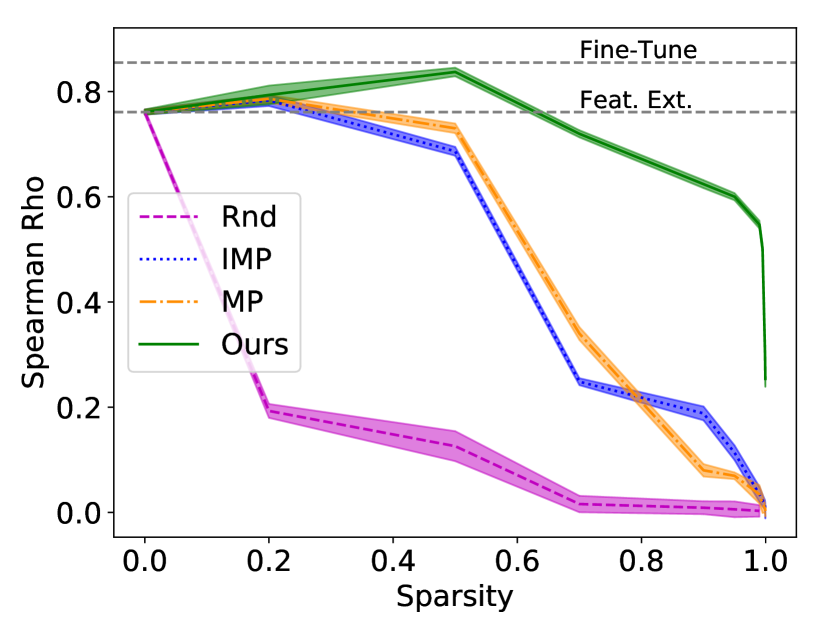
(a) STS-B

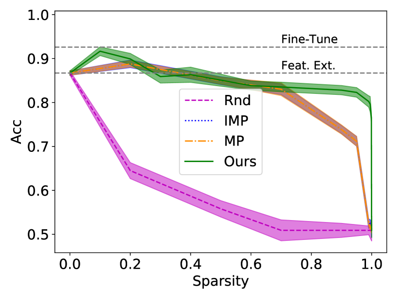
(b) SST-2

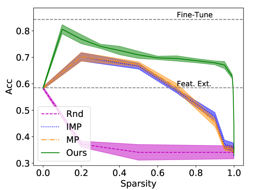
(c) MNLI

Figure 2: Comparison of multiple model adaptation and pruning methods. All results are averaged over five runs with different random seeds; shaded areas represent the corresponding standard deviations. Detailed performance can be found in the Supplementary Material.

Fig. 2 compares the performance of our approach and other model adaptation and pruning methods. Compared to feature-extraction, in all three tasks, our method can obtain sparse networks with significantly better performance; particularly, in MNLI, our method can prune up to 99.5% parameters of BERT while reaching better or comparable performance. Compared to fine-tuning, our method can extract sub-networks with comparable performance, without statistically significant gaps in STS-B and SST-2. These observations suggest that our method shares the advantages of feature extraction and fine-tuning (re-use weights and structures), but can also reduce the model size (see Table 1).

As for the pruning strategies, to ensure fair comparison, we keep all un-pruned weights from BERT with their original values (see the bottom row in Fig. 1). We find that the performance of all pruning methods drops as the sparsity level increases, but our method outputs the best-performing sub-networks across all sparsity levels and tasks, and the performance gap is significant under most conditions. Furthermore, the performance of our method is more robust to the growth of sparsity: the other pruning methods encounter a rapid performance drop when the sparsity reaches 0.5 – 0.7, but our method mostly remains its performance until the sparsity reaches 0.95. These observations show that our approach can consistently produce (near-)optimal supermasks for BERT (see §3).

4.2 Topological Analysis

In this subsection, we inspect the topological differences between supermasks (obtained by our method) and task-specific winning tickets (obtained by IMP/IMP). Fig. 3 shows that that, even at the same sparsity levels, supermasks are substantially different from winning tickets, in terms of layer-wise sparsity and component-wise sparsity. For example, at sparsity 0.2 (top row in Fig. 3), IMP/MP prunes more weights in the embedding layer and fewer in the Transformer layers and components; but at higher sparsity levels (0.99, bottom row in Fig. 3), the pattern is reversed: compared to IMP/MP, our method prunes more weights in the embedding layers and fewer in Transformer layers. Similar observations can be made consistently across all selected GLUE tasks. These results suggest that (i) the topological structures of supermasks and winning tickets are very different, and (ii) the topological differences should follow from differences in the pruning strategy rather than differences in the downstream tasks. The causality and relation between layer/component-wise sparsity and the model performance is worth further investigation, and we leave it for future work.

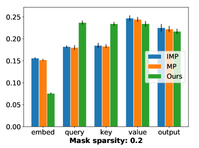
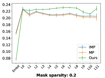
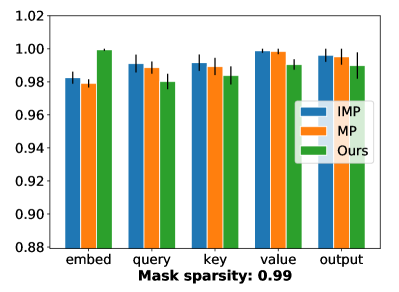
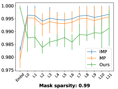
Figure 3: The distribution of the surviving connections over different components (left) and layers (right) is different in the sub-networks obtained through our approach or MP/IMP. Results obtained from five runs on MNLI. Results for the other datasets are in Supplementary Material. Error bars: standard deviation.

Spa-	STS-B (rho)		SST-2 (acc)		MNLI (acc)
rsity	Shufl	Reinit	Shufl	Reinit	Shufl	Reinit
0.2	.397	0.05	.826	.491	.714	.328
0.5	.312	-.019	.808	.491	.601	.328
0.7	.282	.006	.787	.491	.554	.328
0.9	.268	-.036	.720	.491	.403	.328
0.95	.213	.008	.589	.491	.318	.328
0.99	.155	-.016	.509	.491	.353	.328
0.999	.011	.005	.509	.491	.343	.328

Table 3: Supermasks are sensitive to shuffling and weight re-initialisation. For re-initialisation, each pre-trained weight is multiplied with a random value drawn from normal distribution $\mathcal{N}(1,\sigma)$, where $\sigma=0.01$. Performance with $\sigma=0.1$ and $0.001$ are similar.

4.3 Ablation Study

To further understand what contributes to the strong performance of supermasks obtained by our method, we perform multiple ablation study in this subsection.

Sensitivity Test

Winning tickets obtained by IMP and MP are sensitive to mask shuffling (where the surviving connections of a given layer are randomly redistributed over that layer) and weight re-initialisation (where $w_{0}$ is rescaled before fine-tuning) Frankle and Carbin (2019); Frankle et al. (2020b). We test whether supermasks share these characteristics by performing shuffling and re-initialisation operations on the obtained supermasks, applying the new masks to BERT and re-update the weights in the task-specific MLP. From Table 3, it is clear that supermasks are sensitive to shuffling and, especially, weight re-initialisation; even small disturbance on the weights drops the performance to near-random level. This finding suggests that our method is able to pick the most important weights in the original model (c.f., Frankle et al. (2020b)).

Connection Recovery

In IMP/MP, if a weight is pruned in an early stag, it will remain pruned in all follow-up steps. In our algorithm, negative elements of $\theta$ can become positive at later stages. Hence, our method allows for pruned network connections to be reactivated while IMP/MP does not.

A considerable percentage of weights are reactivated in our algorithm: for example, in a sparsity-0.99 sub-network obtained by our method on MNLI, 12.3% of its connections were recovered from the connections pruned in early stages. To study how weight reactivation affects the performance of supermasks, we revise Alg. 1 so that elements that become negative are forced to remain negative in all following SGD steps. Performance of the revised algorithm is presented in Table 4. Disabling connection recovery significantly harms the performance across all tasks and sparsity levels. With the growth of sparsity, the performance loss also increases, suggesting that connection recovery is particularly important for obtaining good high-sparsity models. We believe this also explains the observation from Fig. 2 that the gap between our method and IMP/MP increases with the growth of sparsity.

	STS-B		SST-2		MNLI
Sparsity	Rho	$\Delta$	Acc	$\Delta$	Acc	$\Delta$
0.2	.768	-.026	.860	.-.048	.742	-.027
0.5	.804	-.033	.815	.-.041	.690	-.019
0.7	.628	-.092	.803	-.040	.653	-.043
0.9	.563	-.061	.790	-.046	.628	-.051
0.95	.519	-.081	.783	-.048	.621	-.050
0.99	.417	-.013	.759	-.051	.575	-.053
0.999	.066	-. 235	.671	-.101	.333	-.113

Table 4: Disabling connection recovery harms the performance. $\Delta$: performance difference caused by disabling recovery, compared to sub-networks obtained by the standard Alg. 1 at the same sparsity.

5 Conclusion

In this work, we proposed a novel paradigm to adapt pre-trained models to downstream tasks, which prunes task-irrelevant connections while keeping all remaining weights intact. We formulated the pruning problem as an optimisation problem and proposed an efficient algorithm to obtain the (near-)optimal sub-networks. Experiments on BERT showed that our method can achieve highly competitive performance on downstream tasks, even without fine-tuning. As it reuses the original architecture and weight values, our method is particularly suitable for adapting a base model to downstream tasks with minimum extra data to download. Moreover, pruning all task-irrelevant connections may help understand what are the ‘core’ neural connections of the pre-trained models and provide inspirations to design new neural architectures.

References

- Blalock et al. (2020) Davis Blalock, Jose Javier Gonzalez Ortiz, Jonathan Frankle, and John Guttag. 2020. What is the state of neural network pruning? arXiv:2003.03033.
- Brix et al. (2020) Christopher Brix, Parnia Bahar, and Hermann Ney. 2020. Successfully applying the stabilized lottery ticket hypothesis to the transformer architecture. In ACL.
- Cao et al. (2020) Qingqing Cao, Harsh Trivedi, Aruna Balasubramanian, and Niranjan Balasubramanian. 2020. DeFormer: Decomposing pre-trained Transformers for faster question answering. In ACL.
- Chen et al. (2020) Tianlong Chen, Jonathan Frankle, Shiyu Chang, Sijia Liu, Yang Zhang, Zhangyang Wang, and Michael Carbin. 2020. The lottery ticket hypothesis for pre-trained BERT networks. In NeurIPS.
- Colombo and Gao (2020) Nicolo Colombo and Yang Gao. 2020. Disentangling neural architectures and weights: A case study in supervised classification. arXiv:2009.05346.
- Courbariaux et al. (2015) Matthieu Courbariaux, Yoshua Bengio, and Jean-Pierre David. 2015. Binaryconnect: Training deep neural networks with binary weights during propagations. In NeurIPS.
- Devlin et al. (2019) Jacob Devlin, Ming-Wei Chang, Kenton Lee, and Kristina Toutanova. 2019. BERT: pre-training of deep bidirectional transformers for language understanding. In NAACL.
- Fan et al. (2020) Angela Fan, Pierre Stock, Benjamin Graham, Edouard Grave, Rémi Gribonval, Herve Jegou, and Armand Joulin. 2020. Training with quantization noise for extreme model compression. In ICLR.
- Frankle and Carbin (2019) Jonathan Frankle and Michael Carbin. 2019. The lottery ticket hypothesis: Finding sparse, trainable neural networks. In ICLR.
- Frankle et al. (2020a) Jonathan Frankle, Gintare Karolina Dziugaite, Daniel M. Roy, and Michael Carbin. 2020a. Linear mode connectivity and the lottery ticket hypothesis. In ICML.
- Frankle et al. (2020b) Jonathan Frankle, Gintare Karolina Dziugaite, Daniel M. Roy, and Michael Carbin. 2020b. Pruning neural networks at initialization: Why are we missing the mark? arXiv:2009.08576.
- Gale et al. (2019) Trevor Gale, Erich Elsen, and Sara Hooker. 2019. The state of sparsity in deep neural networks. arXiv:1902.09574.
- Ganesh et al. (2020) Prakhar Ganesh, Yao Chen, Xin Lou, Mohammad Ali Khan, Yin Yang, Deming Chen, Marianne Winslett, Hassan Sajjad, and Preslav Nakov. 2020. Compressing large-scale transformer-based models: A case study on BERT. arXiv:2002.11985.
- Gordon et al. (2020) Mitchell A. Gordon, Kevin Duh, and Nicholas Andrews. 2020. Compressing BERT: studying the effects of weight pruning on transfer learning. In RepL4NLP@ACL.
- He et al. (2016) Kaiming He, Xiangyu Zhang, Shaoqing Ren, and Jian Sun. 2016. Deep residual learning for image recognition. In CVPR.
- Houlsby et al. (2019) Neil Houlsby, Andrei Giurgiu, Stanislaw Jastrzebski, Bruna Morrone, Quentin de Laroussilhe, Andrea Gesmundo, Mona Attariyan, and Sylvain Gelly. 2019. Parameter-efficient transfer learning for NLP. In ICML.
- Lan et al. (2020) Zhenzhong Lan, Mingda Chen, Sebastian Goodman, Kevin Gimpel, Piyush Sharma, and Radu Soricut. 2020. ALBERT: A lite BERT for self-supervised learning of language representations. In ICLR.
- Li et al. (2017) Hao Li, Soham De, Zheng Xu, Christoph Studer, Hanan Samet, and Tom Goldstein. 2017. Training quantized nets: A deeper understanding. In NeurIPS.
- Peters et al. (2019) Matthew E. Peters, Sebastian Ruder, and Noah A. Smith. 2019. To tune or not to tune? adapting pretrained representations to diverse tasks. In RepL4NLP.
- Ramanujan et al. (2020) Vivek Ramanujan, Mitchell Wortsman, Aniruddha Kembhavi, Ali Farhadi, and Mohammad Rastegari. 2020. What’s hidden in a randomly weighted neural network? In CVPR.
- Rebuffi et al. (2017) Sylvestre-Alvise Rebuffi, Hakan Bilen, and Andrea Vedaldi. 2017. Learning multiple visual domains with residual adapters. In NeurIPS.
- Savarese et al. (2020) Pedro Savarese, Hugo Silva, and Michael Maire. 2020. Winning the lottery with continuous sparsification. In NeurIPS.
- Shen et al. (2020) Sheng Shen, Zhen Dong, Jiayu Ye, Linjian Ma, Zhewei Yao, Amir Gholami, Michael W. Mahoney, and Kurt Keutzer. 2020. Q-BERT: Hessian Based Ultra Low Precision Quantization of BERT. In AAAI.
- Wang et al. (2019) Alex Wang, Amanpreet Singh, Julian Michael, Felix Hill, Omer Levy, and Samuel Bowman. 2019. GLUE: A multi-task benchmark and analysis platform for natural language understanding. In ICLR.
- Wortsman et al. (2020) Mitchell Wortsman, Vivek Ramanujan, Rosanne Liu, Aniruddha Kembhavi, Mohammad Rastegari, Jason Yosinski, and Ali Farhadi. 2020. Supermasks in superposition. In NeurIPS.
- Zhang et al. (2020) Tianyi Zhang, Felix Wu, Arzoo Katiyar, Kilian Q. Weinberger, and Yoav Artzi. 2020. Revisiting few-sample BERT fine-tuning. arXiv:2006.05987.
- Zhou et al. (2019) Hattie Zhou, Janice Lan, Rosanne Liu, and Jason Yosinski. 2019. Deconstructing lottery tickets: Zeros, signs, and the supermask. In NeurIPS.
- Zhu and Gupta (2018) Michael Zhu and Suyog Gupta. 2018. To prune, or not to prune: Exploring the efficacy of pruning for model compression. In ICLR Workshop Track.