Quantify the Non-Markovian Process with Intervening Projections in a Superconducting Processor

Abstract

A Markov assumption considers a physical system memoryless to simplify its dynamics. Whereas memory effect or the non-Markovian phenomenon is more general in nature. In the quantum regime, it is challenging to define or quantify the non-Markovianity because the measurement of a quantum system often interferes with it. We simulate the open quantum dynamics in a superconducting processor, then characterize and quantify the non-Markovian process. With the complete set of intervening projections and the final measurement of the qubit, a restricted process tensor can be determined to account for the qubit-environment interaction. We apply the process tensor to predict the quantum state with memory effect, yielding an average fidelity of $99.86\%\pm 1.1\permil$. We further derive the Choi state of the rest process conditioned on history operations and quantify the non-Markovianity with a clear operational interpretation.

I Introduction

Schrödinger equation can formulate the evolution of a quantum system whose state is isolated. A realistic quantum system is unavoidably coupled to environment, which typically contains many degrees of freedom and hard to characterize and control [1, 2, 3]. The dynamics of this open quantum system sometimes can be simplified with a Markov assumption, such as in the Gorini-Kossakowski-Sudarshan-Lindblad (GKSL) master equation [4, 5, 6]. It assumes that the environment is stationary and the system-environment interaction is weak and uncorrelated. Mathematically, a Markov evolution generated by the GKSL master equation is composed of a series of completely positive trace-preserving (CPTP) maps, which form a semi-group [5, 7].

If the evolution of a quantum system depends not only on its instantaneous state but also on history, it is considered non-Markovian or has memory effects. The information of the process history can be stored somewhere and retrieved later to affect the system. The non-Markovian behavior in the quantum regime is challenging to define and quantify, mostly because that general measurements of a quantum system will unavoidably interfere with it [8, 9]. With the advance of quantum device and control apparatus, the revealing of the non-Markovian effects have been constantly reported  [10, 11, 12, 13, 14, 15]. Previous studies of non-Markovianity mainly characterize the open dynamics with the final tomographic measurement, i.e. the observer only waits at the end of the stochastic process to measure the mixed quantum state, and the non-Markovianity is revealed by examining the state changes over a series of time steps. In general, there are two kinds of approaches to characterizing the non-Markovianity  [16, 17, 11, 12, 13, 18, 19, 20, 21]. One is to detect the information flow between the system and its environment. The other is to check the divisibility of the dynamical map.

Although previous experiments have shown evidence of the quantum non-Markovian process, there is no consensus on the quantification of memory effect [9, 22]. The observations also lacks a clear causal structure [23, 24]. Here in this work, we apply an alternative method to characterize and quantify the non-Markovian process with intervening projective measurements, or positive operator-valued measurements (POVMs) [1]. The projections are not only the final measurement but also active interrogations on each intermediate step of the process. This method is feasible because that projective measurements can be integrated as local operators in the tomographic process tensor framework  [25, 26]. Experimentally, we design a three-time-step open quantum process in a superconducting processor, where standard two-qubit gates are selected to simulate the system-environment interaction. We implement arbitrary POVMs by using the field-programmable-gate-array (FPGA)-based fast measurement and control hardware and customized quantum instruction set architecture (ISA) [27]. The restricted process tensor is determined using a complete set of POVMs. The intervening projective measurements reveal the information of the instantaneous state, and at the same time refresh the system deterministically, from which we can compare the causal relation on different time steps.

Note that a process tensor has been experimentally determined with unitary gates on IBM’s cloud-based quantum processors [28]. Their work traces the information flow between different stages of the process, and provides the lower bounding of the memory effect. Here since projective measurements destroy the system-environment entanglement and steer the system into a definite pure state that is independent of its previous trajectories, we can check if there is a conditional dependence of the future dynamics on the past control operations [9, 26]. Consequently, we can directly determine whether a process is Markovian or non-Markovian in a finite number of experiments. With projective measurements providing complete information of the system during the process, we finally quantify the non-Markovian process in a smaller subset of time steps conditioned on earlier operations. Based on our experiment, we illustrate the operational interpretation of the non-Markovianity.

II Open Quantum Dynamics Described by the Tensor Network

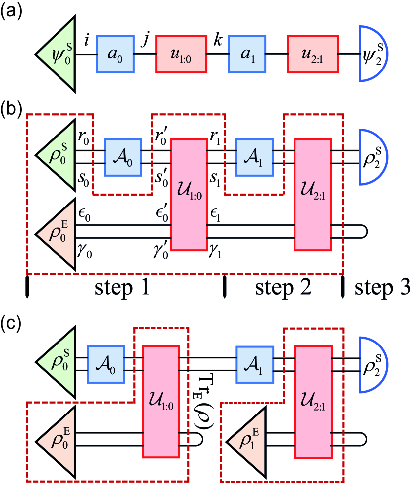
Figure 1: Tensor diagrams of the three-time-step process, including initial states of the system $\mathrm{\mathbf{S}}$ (green triangle) and the environment $\mathrm{\mathbf{E}}$ (orange triangle), intervening local operators (blue box) and $\mathrm{\mathbf{SE}}$ interactions (red rectangle). (a) Closed dynamics of a single qubit $\mathrm{\mathbf{S}}$. (b) Process tensor depiction of the open quantum dynamics. The process tensor $\mathbf{\mathcal{T}}^{2:0}$ encodes all the environmental information in the dashed frame. (c) Traditional depiction of the open quantum dynamics, represented by a concatenation of CPTP maps. For each step, the dynamics of $\mathrm{\mathbf{S}}$ is simulated by the reduced $\mathrm{\mathbf{SE}}$ unitary evolution (outlined in the dashed frame).

We here use the mathematical tool of tensor network [29, 30] to describe the quantum process. In a simplified situation [Fig. 1(a)], a complex vector describes the pure state of a qubit system $\mathrm{\mathbf{S}}$. It can be equivalently denoted by a tensor $(\psi_{0})_{i}$ with one index $\textit{i}=$0 or 1, encoding the ground or excited state. At each time step $n$, the system evolution can be represented by a tensor $(\mathbf{u}_{n:n-1})^{j}_{k}$, while an observer intervenes in the trajectory with a local operator $(\mathbf{a}_{n-1})^{i}_{j}$. The dynamics of $\mathrm{\mathbf{S}}$ can be simulated by summing over the corresponding tensor indexes, called a ‘tensor contraction’ [31].

For an open quantum system, we design a process where a single qubit $\mathrm{\mathbf{S}}$ interacts with its environment [Fig. 1(b)]. The state of $\mathrm{\mathbf{S}}$ under stochastic quantum evolution is now represented by a density matrix $\rho^{\mathrm{S}}_{s_{0},r_{0}}$. In our superconducting processor, we choose a neighboring ancilla qubit $\mathrm{\mathbf{E}}$ to simulate the environment of $\mathrm{\mathbf{S}}$. Initially, $\mathrm{\mathbf{S}}$ and $\mathrm{\mathbf{E}}$ are prepared to a tensor product of the ground states, $\rho^{\mathrm{SE}}_{s_{0},r_{0};\gamma_{0},\epsilon_{0}}=\rho^{\mathrm{S}}_{s_{0},r_{0}}\otimes\rho^{\mathrm{E}}_{\gamma_{0},\epsilon_{0}}=|00\rangle$. The intervened local operator on $\mathrm{\mathbf{S}}$ is represented by a tensor $\mathcal{A}^{s_{0},r_{0}}_{s^{\prime}_{0},r^{\prime}_{0}}$, and the $\mathrm{\mathbf{SE}}$ interaction is represented by a tensor $\mathcal{U}^{s^{\prime}_{0},r^{\prime}_{0};\gamma^{\prime}_{0},\epsilon^{\prime}_{0}}_{s_{1},r_{1};\gamma_{1},\epsilon_{1}}$. This $n$-step quantum process can be simulated by contracting $\rho^{\mathrm{\mathbf{SE}}}$ with sequential $\mathcal{A}$s and $\mathcal{U}$s as following,

$$\rho_{n}{(\mathbf{A}_{n-1:0})} =\operatorname{Tr}_{\mathrm{E}}\left[\mathcal{U}_{n:n-1}\mathcal{A}_{n-1}\cdots\mathcal{U}_{1:0}\mathcal{A}_{0}\left(\rho_{0}^{\mathrm{SE}}\right)\right]$$ (1)

$$=\mathcal{T}^{n:0}\left[\mathbf{A}_{n-1:0}\right].$$ (2)

After tracing out the environment indexes at the final step [Eq. (1)], we derive the output state of $\mathrm{\mathbf{S}}$. Consequently, there is a map from the sequence of local operators $\{\mathcal{A}_{0},\cdots,\mathcal{A}_{n-1}\}$ ($\mathbf{A}_{n-1:0}$ for short) to the output state $\rho_{n}$. This map is coined a ‘quantum comb’ in the quantum circuit architecture [32], or a ‘process tensor’ in open quantum dynamics [25].

The process tensor encodes the hidden environmental information in the dashed frame of Fig. 1(b). In Eq. (2), $\mathbf{\mathcal{T}}^{n:0}$ is a multilinear map on $\mathbf{A}_{n-1:0}$, i.e. its linearity holds independently to the operator $\mathcal{A}$ at each step. Then $\mathcal{T}^{n:0}$ can be experimentally determined by the quantum tomography technique [33]. At step $n$, the local operator can be uniquely decomposed by a fixed set of linearly independent basis operators $\{\mathcal{B}_{l}\}$, $\mathcal{A}_{n-1}=\sum_{l}(\beta_{n-1})_{l}\mathcal{B}_{l}$. The sequence of local operations can be further expanded in terms of their tensor products,

$$\mathbf{A}_{n-1:0}=\sum_{\vec{l}}\beta_{\vec{l}}\bigotimes_{m=0}^{n-1}(\mathcal{B}_{m})_{l}$$ (3)

where real numbers $\beta_{\vec{l}}$ are the coefficients of the tensor products of $\mathcal{B}s$, and $\vec{l}:=\{l_{0},l_{1},\cdots,l_{n-1}\}$ denotes the combination of operators.

A process tensor has been recently determined using a set of unitary control gates. The tensor can be applied to characterize a non-Markovian process [28]. In this work, we probe the system with intervening projective measurements or POVM operators. Experimentally, our FPGA-based hardware and customized quantum ISA [27] enable us to apply an arbitrary POVM operator on any time step of the process. These POVMs effectively destroy the entanglement between the system and the environment, and steer the system to a definite pure state independent of its previous trajectories [9]. With a complete set of POVM operators $\{\mathcal{P}\}$, a ‘restricted’ process tensor $\mathbf{\mathcal{T}}_{P}$ can be determined [34]. We then derive the process tensor in a subset of steps, which is ‘contained’ in a larger one (the containment property) [25]. With the smaller process tensor, we quantify the system’s non-Markovianity by calculating the von Neumann mutual information [35] of its Choi state [36, 37], and give a clear operational interpretation in the context of our experiment.

III Results

In our experiment, the superconducting quantum processor is a chip composed of six cross-shaped Transmon qubits [38]. The device was mounted in a dilution refrigerator whose base temperature is around 10 mK. We choose two neighboring qubits as the system $\mathrm{\mathbf{S}}$ and the environment $\mathrm{\mathbf{E}}$. They are set at $\omega_{\mathrm{S}}=6.21$ GHz and $\omega_{\mathrm{E}}=5.70$ GHz. The other device parameters are the same as that in Ref. [39]. We specifically design two distinct processes consisting of standard quantum gates in the quantum processor. One has the $\mathrm{\mathbf{SE}}$ interaction brought by a CNOT gate after the first operator and CZ gate the second. We swap these two gates for the other process, where CZ is activated first and CNOT the second.

III.0.1 Implementation of POVMs

The sub-normalized state of the quantum system after a POVM operator $\mathcal{P}$ is given by $\mathcal{P}\rho\mathcal{P}^{\dagger}$, where $\mathcal{P}=|p\rangle\langle p|$ also denotes the state to which we project. The probability of this projection is $\operatorname{Tr}[\mathcal{P}\rho]$. An important consequence of the POVM operator on an open quantum system is the destruction of its entanglement with the environment, as $(\mathcal{P}^{\mathrm{\mathbf{S}}}\otimes\mathcal{I}^{\mathrm{\mathbf{E}}})\rho^{\mathrm{\mathbf{SE}}}(\mathcal{P}^{\mathrm{\mathbf{S}}}\otimes\mathcal{I}^{\mathrm{\mathbf{E}}})=\mathcal{P}^{\mathrm{\mathbf{S}}}\otimes\mathcal{I}^{\mathrm{\mathbf{E}}}\operatorname{Tr}_{\mathrm{\mathbf{S}}}[(\mathcal{P}^{\mathrm{\mathbf{S}}}\otimes\mathcal{I}^{\mathrm{\mathbf{E}}})\rho^{\mathrm{\mathbf{SE}}}]$, where $\mathcal{I}^{\mathrm{\mathbf{E}}}$ is the identity operator on the environment state.

The qubit is usually read out in a superconducting processor by projecting it to the ground state ($\mathcal{P}_{z+}=|0\rangle\langle 0|$) or excited state ($\mathcal{P}_{z-}=|1\rangle\langle 1|$). Whereas in general cases, $\mathcal{P}$ shall project the qubit to any state on the Bloch sphere, which is parameterized as $|p\rangle=\mathrm{cos}\frac{\theta}{2}|0\rangle+e^{i\phi}\mathrm{sin}\frac{\theta}{2}|1\rangle$. Any $\mathcal{P}(\theta,\phi)$ can be realized by introducing the following unitary transformation,

$$\mathcal{P}\rho\mathcal{P}^{\dagger} =(R\mathcal{P}_{z+}R^{\dagger})\rho(R\mathcal{P}_{z+}R^{\dagger})^{\dagger}$$

$$=R(\mathcal{P}_{z+}\operatorname{Tr}[\mathcal{P}_{z+}R^{\dagger}\rho R])R^{\dagger}$$ (4)

where $R(\theta,\phi)$ is a $\theta$-angle rotation around the vector $\vec{n}$ in the $xy$-plane. The azimuth of $\vec{n}$ is $\phi+\pi/2$. As an example, the experimental sequence to implement a POVM operator $\mathcal{P}_{y-}$ is drawn in the dashed frame in Fig. 2(a). We first rotate the qubit by $+\pi/2$ around the $x$-axis. Then we apply a fast dispersive measurement [40] to project it to either the ground state $\mathcal{P}_{z+}$ (the upper ball) or excited state $\mathcal{P}_{z-}$ (the lower ball with lighter color). Finally, we rotate the qubit back to the target state $|p\rangle$ (ball on the rightmost Bloch sphere along the -$y$-axis). Note that in Eq. 4 the probability of $\mathcal{P}$ is calculated by post-selecting [41] the ground-state ($\mathcal{P}_{z+}$). Similarly, we can implement other POVMs to project the qubit onto any axis. $\mathcal{P}_{x+}$ denotes the projection on the positive $x$-axis; $\mathcal{P}_{yz+}$ or $\mathcal{P}_{zy+}$ denotes the projection on the internal ($\theta=-\pi/4$, $\phi=0$) or exterior ($\theta=\pi/4$, $\phi=0$) angle bisector of +$y$ and +$z$ axis; $\mathcal{P}_{yz-}$ is the projection on the reversed direction of $\mathcal{P}_{yz+}$, and so on.

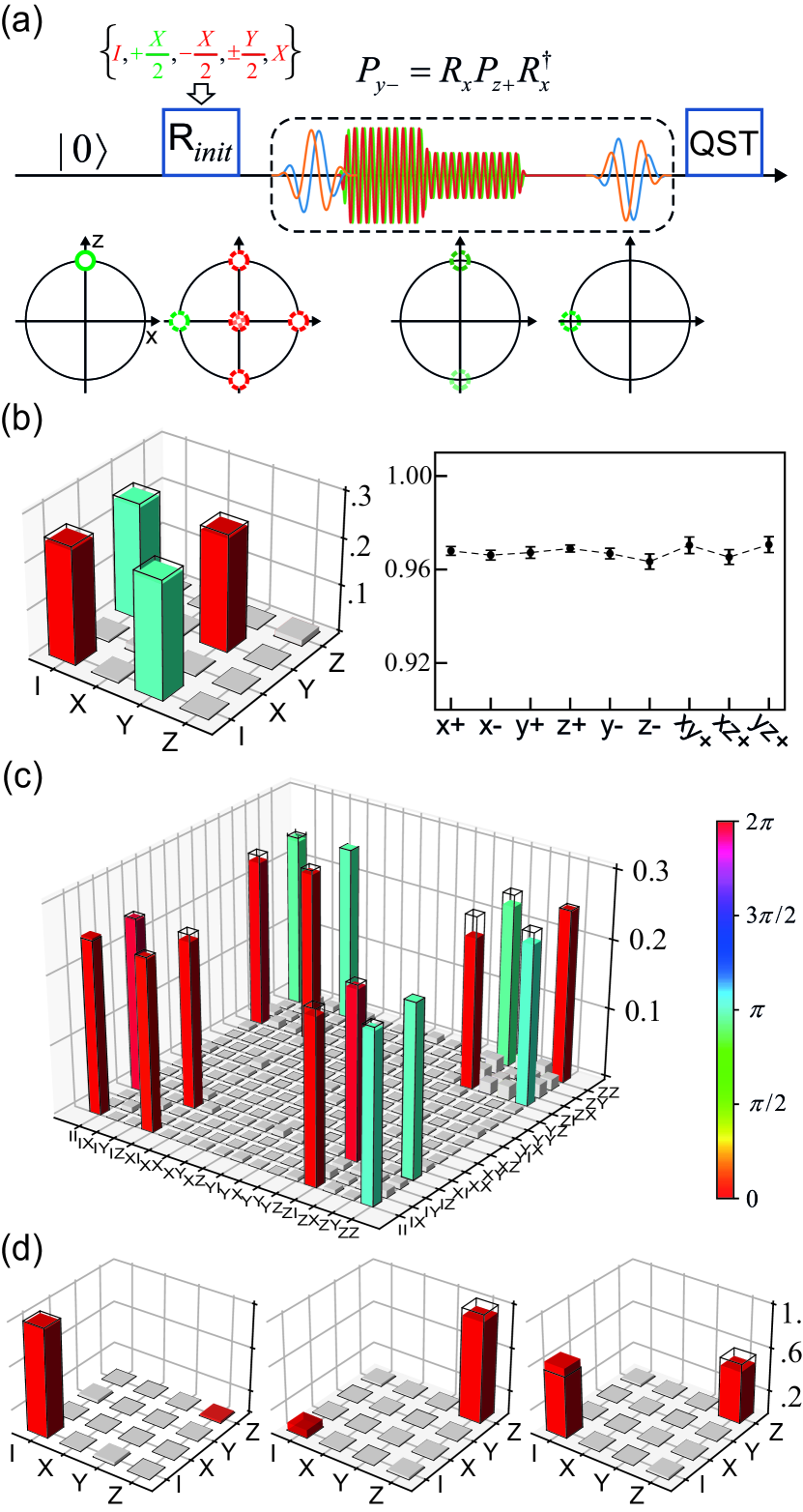
Figure 2: (a) QPT protocol to characterize the $\chi$-matrix of $\mathrm{\mathbf{S}}$, with the implementation of $\mathcal{P}_{y-}$ as an example. (b) Left panel: $\chi$-matrix of $\mathcal{P}_{y-}$. The magnitude and complex phase of $\chi$ elements are shown as the height and color of cubic columns. Magnitudes lower than 0.02 are drawn in gray for visibility. Right panel: QPT fidelities of nine POVMs. (c) $\chi$-matrix of the two-qubit CZ gate. (d) $\chi$-matrices of the reduced CZ-gate, with $\mathrm{\mathbf{E}}$ being prepared to the ground state (left), excited state (middle), and $(|0\rangle-i|1\rangle)/\sqrt{2}$ (right).

III.0.2 Traditional Picture of the Quantum Map

The CPTP map of each step of the process can be equivalently expressed in terms of the Kraus decomposition [1, 35, 42],

$$\Lambda(\rho)=\sum E_{m}\rho E_{n}^{\dagger}\chi_{mn}$$ (5)

where the set of matrices $\{E\}$ are called the Kraus operators of $\Lambda$. To benchmark the quantum gates, QPT protocol are normally used to determine the matrix $\chi_{mn}$ [1, 43]. Here we choose Pauli operators $\{I,\sigma_{x},\sigma_{y},\sigma_{z}\}$ as the Kraus operators. The gate fidelity is calculated by $\operatorname{Tr}[\chi_{\mathrm{ideal}}\chi]$, where $\chi_{\mathrm{ideal}}$ represents an ideal matrix.

We apply the QPT protocol to characterize the POVMs mentioned in Sec. III.0.1. In our experiment, we prepare six qubit states by rotations on the ground state $|0\rangle$. After the process [dashed frame of Fig. 2(a)], the output states are determined using quantum state tomography (QST) [1, 44]. Through out the paper, we use six symmetric POVMs ($\mathcal{P}\{$$x\pm$,$y\pm$,$z\pm\}$) to determine the quantum state, though four informationally complete (IC) POVMs are sufficient [45]. Knowing the input-output relation on a complete set of basis, it is sufficient to determine $\chi$. We can see four bars standing symmetrically on both side of the diagonal of the matrix [left panel of Fig. 2(b)], representing coefficients of[1/4, -1/4, -1/4, 1/4] for Kraus operators [$(I,I)$, $(I,\sigma_{y})$, $(\sigma_{y},I)$, $(\sigma_{y},\sigma_{y})$]. Not surprisingly, the quantum map we determine coincides with $\mathcal{P}_{y-}$,

$$\Lambda_{\mathcal{P}_{y-}}[\rho] \approx\frac{1}{4}(I\rho I-\sigma_{y}\rho I-I\rho\sigma_{y}+\sigma_{y}\rho\sigma_{y})$$

$$=\frac{I-\sigma_{y}}{2}\rho\frac{I-\sigma_{y}}{2}=\mathcal{P}_{y-}\rho\mathcal{P}_{y-}.$$

Note that while the projective measurement is performed along a deterministic axis, the two complementary POVM elements it contains is probabilistic and may not necessarily be trace preserving (TP).

We also characterize other POVMs, which will be used in Sec. III.0.3 as a full basis of operators to determine the process tensor. After normalization, the fidelity of $\mathcal{P}_{y-}$ is 96.9% $\pm$0.12%, averaged over 20 independent QPTs. Fidelities of other POVMs are plotted in the right panel of Fig. 2(b). We have confirmed that the POVM operators are achieved with high fidelities before intervening them in a quantum process to determine the process tensor.

Similarly, we characterize the $\chi$ matrices of the CZ gate [Fig. 2(c)] and CNOT gate (not shown). Their fidelities are $96.3\%\pm 0.29\%$ and $93.1\%\pm 0.53\%$, respectively. We next characterize the quantum map of $\mathrm{\mathbf{S}}$ when it interacts with the ancilla $\mathrm{\mathbf{E}}$, termed the ‘reduced’ quantum map of $\mathrm{\mathbf{S}}$. For CZ gate, the ‘reduced’ map of $\mathrm{\mathbf{S}}$ depends on the state of $\mathrm{\mathbf{E}}$, which can be written as,

$$\Lambda_{\operatorname{Tr}_{\mathrm{\mathbf{E}}}[\mathrm{CZ}]}(\rho^{\mathrm{\mathbf{S}}})=\operatorname{Tr}_{\mathrm{\mathbf{E}}}[\mathcal{U}_{\mathrm{CZ}}\rho^{\mathrm{\mathbf{SE}}}\mathcal{U}^{\dagger}_{\mathrm{CZ}}].$$ (6)

Figure 2(d) displays the $\chi$-matrices of three ‘reduced’ CZ gates with $\mathrm{\mathbf{E}}$ in the ground state ($|0\rangle$), the excited state ($|1\rangle$), and the superposition state ($(|0\rangle-i|1\rangle)/\sqrt{2}$). The equivalent quantum maps are an identity ($I$), a $180^{\circ}$ rotation around the $z$-axis ($Z$), and a complete phase erasing (mixture of $I$ and $Z$ with equal probability), respectively.

III.0.3 Tomography of the Restricted Process Tensor

Following we choose a complete set of basis POVM operators [34],

$$\mathcal{F}=\mathcal{P}{\{x+,x-,y+,z+,y-,z-,xy+,xz+,yz+\}}.$$ (7)

By performing the combinations $\{\mathrm{\mathbf{B}}_{1:0}\}$ = $\bigotimes^{2}\{\mathcal{P}\}$ at the first two steps of the process and measuring the outcome states of $\mathrm{\mathbf{S}}$ using QST, the restricted process tensor can be determined as the following algorithm,

Algorithm Process Tomography of $\mathbf{\mathcal{T}}_{P}^{2:0}$

1:Stats = 3000 $\triangleright$ Repetitions of the sequence

2:$\mathrm{\mathbf{U}}_{2:0}$ = CNOT-CZ or CZ-CNOT $\triangleright$ $\mathrm{\mathbf{SE}}$ interactions

3:$\{\mathrm{\mathbf{B}}_{1:0}\}=\bigotimes^{2}\{P_{x+},P_{x-},P_{y+},\ldots,P_{yz+}\}_{9\times 9}$ $\triangleright$ three-step Basis

4:for $\mathcal{B}_{l_{0}},\mathcal{B}_{l_{1}}$ in $\{\mathrm{\mathbf{B}}_{1:0}\}$ do

5:     for $R_{m}$ in {I, X/2, Y/2, -X/2, -Y/2, X} do $\triangleright$ QST

6:         for i in range(Stats) do

7:              Apply $\mathcal{B}_{l_{0}}$ to $\mathrm{\mathbf{S}}$

8:              Apply $\mathcal{U}_{0}$ to $\mathrm{\mathbf{SE}}$ $\triangleright$ 1st $\mathrm{\mathbf{SE}}$ interaction

9:              Apply $\mathcal{B}_{l_{1}}$ to $\mathrm{\mathbf{S}}$

10:              Apply $\mathcal{U}_{1}$ to $\mathrm{\mathbf{SE}}$ $\triangleright$ 2nd $\mathrm{\mathbf{SE}}$ interaction

11:              Apply $\mathrm{R}_{m}$ to $\mathrm{\mathbf{S}}$

12:              Record the system state of this sequence $S_{\vec{l},m,i}$

13:         end for

14:         Compute the state probability $P_{\vec{l},m}$ from $\{S_{\vec{l},m,i}\}$

15:     end for

16:     Compute the QST result $(\rho_{\vec{l}})_{2\times 2}$ from $\{P_{\vec{l},m}\}$

17:end for

18:Find the solution $(\mathbf{\mathcal{T}}_{P}^{2:0})_{256\times 4}$ as a linear map from $(\mathrm{\mathbf{B}}_{{\vec{l}}})_{9\cdot 9\times 4^{2}\cdot 4^{2}}$ to $(\rho_{{\vec{l}}})_{9\cdot 9\times 2\cdot 2}$

Note we fit the restricted process tensor using the least-square method provided by scientific computing packages [46], and then obtain the best approximation $\mathbf{\mathcal{T}}_{P}$ with positive semi-define constraint and convex optimization (see Sec. III.0.4).

Once a process tensor $\mathbf{\mathcal{T}}_{P}^{2:0}$ is determined, we can predict its output state when arbitrary projections $\mathrm{\mathbf{A}}_{1:0}$ are inserted in the process. The fidelity of predicted state is defined as [47],

$$F(\rho,\sigma)=(\operatorname{Tr}\sqrt{\sqrt{\rho}\sigma\sqrt{\rho}})^{2}$$ (8)

where $\rho$ is the density matrix of $\mathrm{\mathbf{S}}$ measured in experiment, and $\sigma$ is the predicted one. We use an over complete set of $\mathrm{\mathbf{A}}_{1:0}$, consisting of POVMs in $\mathcal{P}\{x+$, $x-$, $y+$, $z+$, $y-$, $z-$, $xy+$, $xz+$, $yz+$, $xy-$, $xz-$, $yz-$, $yx+$, $zx+$, $zy+$, $yx-$, $zx-$, $zy-\}$, to benchmark the process tensor prediction. For comparison, we also use the following traditional quantum map method to predict the quantum process [Fig. 1(c)].

Method Quantum Map of the Markovian System

1:Assume that $\mathrm{\mathbf{S}}$ is initially at the ground state.

2:Calculate the state of $\mathrm{\mathbf{S}}$ after the CP map of $\mathcal{A}_{0}$ using the $\chi$-matrix determined previously [Fig. 2(b)].

3:Calculate the state of $\mathrm{\mathbf{S}}$ after $\mathcal{U}_{1:0}$ using the $\chi$-matrix of the reduced quantum map determined previously.

4:Repeat previous two steps for $\mathcal{A}_{1}$ and $\mathcal{U}_{2:1}$, to obtain the final output state.

Note that in step 3, we choose the reduced map of $\mathcal{U}_{n:n-1}$ conditioned on $\mathrm{\mathbf{E}}$ being in $|0\rangle$. For example, the $\chi$-matrix on the left panel of Fig. 2(d). We assume that $\mathrm{\mathbf{E}}$ remains in $|0\rangle$ throughout the process, which is the Markov assumption widely used to deal with the open quantum dynamics but does not always hold.

In the CNOT-CZ process where CNOT gate is activated at the first step and CZ at the second step, the output states predicted by the process tensor yields extremely high fidelity and stability, averaged to $99.86\%\pm 1.1\permil$ over 20 repetitions. While the traditional quantum map method with the Markov assumption can not accurately predict the output of the process, whose average fidelity is only $80.25\%\pm 13.2\permil$. A second CZ-CNOT process is also characterized for reference. Both methods can well predict the process, whose average fidelities are $99.87\%\pm 1.0\permil$ (process tensor) and $99.76\%\pm 1.5\permil$ (quantum map of the Markovian system).

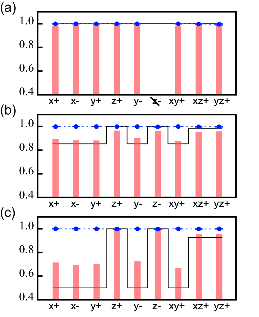
Figure 3: Prediction fidelities of the CNOT-CZ process. We show three representative groups where qubit is firstly projected to three states in the $zy$-plane ($\phi=0$), (a) $\mathcal{A}_{0}=\mathcal{P}_{z+}$ ($\theta=0$), (b) $\mathcal{A}_{0}=\mathcal{P}_{zy+}$ ($\theta=\pi/4$), (c) $\mathcal{A}_{0}=\mathcal{P}_{y-}$ ($\theta=\pi/2$). Prediction fidelities of process tensor method (blue dot) and traditional quantum map method (solid bar) are drawn on the horizontal axis for different second-step projections $\mathcal{A}_{1}$. Theoretical result of the second method is calculated with all gates ideal (black line). Note that one fidelity is omitted when projections are chosen as $\mathcal{A}_{1:0}$ = $\mathcal{P}_{z+}$-$\mathcal{P}_{z-}$ because the measurement probability is close to zero. In other words, this trajectory is forbidden in this process.

To study how the previous trajectory of the system affects the subsequent dynamics, partial results of the CNOT-CZ process are presented in Fig. 3. The fidelity of predicted states are grouped by different choices of $\mathcal{A}_{0}$: $\mathcal{P}_{z+}$[Fig. 3(a)], $\mathcal{P}_{zy+}$[Fig. 3(b)], $\mathcal{P}_{y-}$[Fig. 3(c)]. We can distinguish the non-Markovian trajectories by checking the discrepancies of the fidelity. For example, if we fix the second-step projection to $\mathcal{P}_{x+}$, the Markov predictions (quantum map method) are unchanged because the reduced CZ gate is actually an identity map on $\mathrm{\mathbf{S}}$ [left panel of Fig. 2(d)]. However, the distances between the unchanged state ($\sigma$=$\mathcal{P}_{x+}$) and the three experimental measured $\rho$ are different, indicating the change of the final state. Clearly, the second-step trajectory of $\mathrm{\mathbf{S}}$ depends on the the first-step operation $\mathcal{A}_{0}$, a distinguishing feature of non-Markovianity. In other words, the system dynamics is affected by the history of operations on it. For the CZ-CNOT process, however, we can not find any evident changes of the second-step quantum trajectory conditioned on different $\mathcal{A}_{0}$. This means that the CZ-CNOT process is almost Markovian. Note that the visibility of non-Markovianity in experiment (solid-red bar) is lower than the ideal one (black reference line). This is because that both $\mathrm{\mathbf{S}}$ and $\mathrm{\mathbf{E}}$ in our processor dissipate to a larger lossy environment. For qubit $\mathrm{\mathbf{S}}$, the measured state and the predicted state shrink to the north pole of the Bloch sphere, leading to a closer distance in between. For qubit $\mathrm{\mathbf{E}}$, it relaxes to the ground state during the process, losing some memory.

III.0.4 Quantify the Non-Markovianity

We further quantify the non-Markovianity of the process. With recorded results of a complete set of POVMs on each step (Sec. III.0.3), we can vary the first-step POVM operator $\mathcal{P}(\theta,0)$ and derive the rest process tensor, parameterized as $\mathbf{\mathcal{T}}_{P}^{2:1}(\theta)$. The azimuth angle $\phi$ is set to zero, i.e. all states of $\mathrm{\mathbf{S}}$ after the first projections are in the $zy$ plane.

The non-Markovian evolution of a system are held in the process tensor $\mathbf{\mathcal{T}}_{P}$, which can be conveniently rewritten as a many-body generalized Choi state $\Upsilon$ using the ‘Choi-Jamiołkowski’ representation [37]. Here we choose to gauge the non-Markovianity by the von Neumann mutual information [35] in $\Upsilon$, which can also be viewed as the distance between $\Upsilon$ and its uncorrelated state $\Upsilon_{\mathrm{\otimes}}$. The distance is calculated by the von Neumann relative entropy,

$$\mathcal{D}(\Upsilon\|\Upsilon_{\mathrm{\otimes}})=\operatorname{Tr}\left[\Upsilon(\operatorname{ln}\Upsilon-\operatorname{ln}\Upsilon_{\mathrm{\otimes}})\right].$$ (9)

In our experiment, the Choi state of the last-step process is denoted by $(\Upsilon^{2:1})_{4^{1}\cdot 2\times 4^{1}\cdot 2}$, with subscripts for its dimensions. The uncorrelated state $\Upsilon^{2:1}_{\mathrm{\otimes}}$ represents the last-two-step process with a Markov assumption [Fig. 2(c)]. We calculate it as the tensor product of the average initial state of $\mathrm{\mathbf{S}}$ and the Choi state of the reduced quantum map (conditioned on the average state of $\mathrm{\mathbf{E}}$),

$$(\Upsilon^{2:1}_{\mathrm{\otimes}})_{4\cdot 2\times 4\cdot 2}=(\Lambda^{2:1})_{4\times 4}\otimes(\rho_{1})_{2\times 2}.$$ (10)

Care should be taken when deriving the restricted process tensor $\mathbf{\mathcal{T}}_{P}^{2:1}$, because it is under-determined using only POVMs. The solutions may not always be positive semi-define (PSD). In contrast, on the set of complete basis including both projective measurement and unitary control, the full process tensor is well-determined and PSD [25]. Here we use an optimization method to minimize the non-Markovianity of $\Upsilon^{2:1}$ in the space spanned by POVMs with the PSD constraint. The procedure to derive $\mathcal{N}^{2:1}$ is illustrated in the left panel of Fig. 4(a). The restricted process tensor determined by projective measurements is defined in a linear space spanned by the POVM operators ($\mathrm{\mathbf{PM}}$, dashed-blue line). It contains a smaller space of process tensors whose Choi states are PSD (solid-orange area). In the optimization method, we first find an initial solution $\Upsilon^{2:1}_{0}$ (black dot) using the least-square fitting, and then progressively optimize the Choi state $\Upsilon^{2:1}$ by minimizing the distance [Eq. 9] to its uncorrelated state (cross circle $\otimes$) [Eq. 10]. We take the minimal distance as the measure of non-Markovianity $\mathcal{N}^{2:1}$,

$$\mathcal{N}^{2:1}=\min_{\Upsilon^{2:1}\in{\{PSD\}}}\mathcal{D}(\Upsilon^{2:1}\|\Upsilon^{2:1}_{\mathrm{\otimes}}).$$ (11)

The result of Eq. 11 converges to the point (black cross) that has the minimal distance to $\Upsilon^{2:1}_{\mathrm{\otimes}}$.

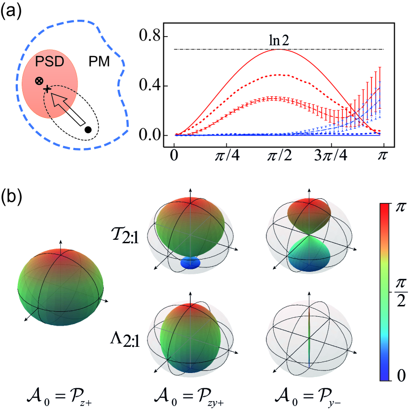
Figure 4: (a) Left panel: space where the last-two-step restricted process tensor is defined. The arrow shows the optimization procedure, starting from an initial value (black dot), to one point $\Upsilon^{2:1}$ (black cross) that is closet to the uncorrelated Choi state $\Upsilon^{2:1}_{\mathrm{\otimes}}$ (cross circle). Right panel: the non-Markovianity of the last-two-step process conditioned on different first-step POVMs parameterized with $\theta$. The CNOT-CZ process yields the maximum non-markovianity when $\theta=\pi/2$. The experimental result (red dashed line) is lower than the ideal case (red solid line). Numerical simulations considering dissipation of both $\mathrm{\mathbf{S}}$ and $\mathrm{\mathbf{E}}$ (red dotted line) accounts for the trend. The other CZ-CNOT process is almost Markovian and memoryless (blue lines). (b) Volumes of the accessible states of $\mathrm{\mathbf{S}}$. At the beginning of the second step of CNOT-CZ process, POVM operators spans the states all around the Bloch sphere (left volume). When the first-step projection $\mathcal{A}_{0}$ is $\mathcal{P}_{z+}$, the final state of the process is unchanged (Identity to $\mathcal{A}_{1}$), well predicted by both methods. When $\mathcal{A}_{0}$ is $\mathcal{P}_{zy+}$ or $\mathcal{P}_{y-}$, the process tensor $\mathbf{\mathcal{T}}_{2:1}$ and the quantum map $\mathbf{\Lambda}_{2:1}$ generate the output of the process differently. We color the states according to the projection angle $\theta$ of $\mathcal{A}_{1}$.

The right panel of Fig. 4(b) shows the results of $\mathcal{N}^{2:1}$ versus different choices of the first-step operator ${\mathcal{P}(\theta,0)}$. For the CNOT-CZ process, it yields the maximum non-Markovianity when $\theta$=$\frac{\pi}{2}$ (red dashed line). On the contrary, the CZ-CNOT process does not produce significant non-Markovianity (blue dashed line) whatever $\mathcal{A}_{0}$ we choose. As we conclude in Sec. III.0.3, the CZ-CNOT process is almost Markovian.

Note that non-Markovianity of the CNOT-CZ process in the real quantum processor (red dashed line) shows a lowered visibility compared with the ideal theoretical result (red solid line). Similar to the observation in Sec. III.0.3, this lowered visibility is due to the dissipation of both $\mathrm{\mathbf{S}}$ and $\mathrm{\mathbf{E}}$ to a larger environment. We numerically calculate $\mathbf{\mathcal{T}}_{P}^{2:0}$ using the non-ideal CNOT and CZ gates that we have experimentally characterized, and then derive the $\mathcal{N}^{2:1}$s versus $\theta$ (red dotted line), from which the trend can be partially verified. The even lower value of $\mathcal{N}^{2:1}$ is most likely caused by other noises, such as the phase noise of a ‘mediocre’ clock when qubit sequence gets longer [48], and the photon number fluctuations noise during the projective measurement [49, 50].

Both processes show a larger standard deviation when $\theta$ gets bigger. This is because that we have normalized the Choi state by dividing the probability of $\mathcal{A}_{0}$, which reduces to 0 as $\theta$ gets close to $\pi$. $\mathcal{N}^{2:1}$s of both processes also get higher when $\theta$ approaches to $\pi$. This indicates that some memory sources are not included in the simple two-qubit model when $\mathrm{\mathbf{S}}$ is projected to a higher population of excited-state. Some possible candidates are the measurement induced state transitions [51] and the crosstalk from neighboring qubit. Nevertheless, such temporal correlation effects will be absorbed in the process tensor, which can accurately predict the non-Markovian process (Sec. III.0.3).

To illustrate the operational meaning of $\mathcal{N}^{2:1}$, we analyze the cause of non-Markovianity in the CNOT-CZ process. At the beginning of the first process, $\mathrm{\mathbf{E}}$ is reset to $|0\rangle$. After one of the first projections $\mathcal{P}_{z+}$, $\mathcal{P}_{zy+}$, or $\mathcal{P}_{y-}$, the state of $\mathrm{\mathbf{S}}$ changes to either $|0\rangle$, $\mathrm{cos}\frac{\pi}{8}|0\rangle-i\mathrm{sin}\frac{\pi}{8}|1\rangle$, or $(|0\rangle-i|1\rangle)/{\sqrt{2}}$. Correspondingly, the state of $\mathrm{\mathbf{SE}}$ changes after the CNOT gate to either a product state $|00\rangle$, a partial entangled state $\mathrm{cos}\frac{\pi}{8}|00\rangle-i\mathrm{sin}\frac{\pi}{8}|11\rangle$, or a maximum entangled state (MES) $(|00\rangle-i|11\rangle)/\sqrt{2}$. As has been studied in Refs. [34, 52, 11, 26], initial correlations between a system $\mathrm{\mathbf{S}}$ and its environment $\mathrm{\mathbf{E}}$ carries historical information and will affect its dynamics at a later time. At the beginning of the second step, the complete set of POVMs $\mathcal{A}_{1}$ (after normalization) effectively spans the state all around the Bloch sphere, [left volume in Fig. 4(b)]. The process tensor and the quantum map method describe the following process differently. We present the volume changes of the set of accessible states of $\mathrm{\mathbf{S}}$ after the CZ gate in fig. 4(b). We first check the quantum map method. When the $\mathrm{\mathbf{SE}}$ state is $|00\rangle$, the reduced CZ gate is effectively an identity gate, leaving the states unchanged (left volume). When the $\mathrm{\mathbf{SE}}$ state is partially entangled ($\mathrm{cos}\frac{\pi}{8}|00\rangle-i\mathrm{sin}\frac{\pi}{8}|11\rangle$), some of the phase information of $\mathrm{\mathbf{S}}$ is lost statistically after the quantum map and the volume of states shrinks toward the $z$-axis (middle lower volume). An extreme case is when $\mathrm{\mathbf{SE}}$ is initially in MES. Phase information of $\mathrm{\mathbf{S}}$ is completely erased through the map, and all output states goes to the $z$-axis (right lower volume). Quite differently, the process tensor ‘knows’ how $\mathrm{\mathbf{S}}$ and $\mathrm{\mathbf{E}}$ are correlated after $\mathcal{A}_{1}$, which breaks the entanglement and projects $\mathrm{\mathbf{S}}$ to a predefined state. Thus the last-two-step process is more accurately described with tensor operators. The volume of accessible state predicted by the process tensor [right upper volumes in Fig. 4(b)] differs most with that of the quantum map when $\mathrm{\mathbf{SE}}$ is initially in MES. This, in turn, is consistent with the non-Markovianity obtained in Fig. 4(a). We will most unlikely to confuse the last-two step process to be Markovian, if we apply $\mathcal{P}_{y-}$ at the first step and compare the output states with the Markov predictions. The theoretical value (red solid line) approaching $\ln{2}$ means that the maximum probability of not finding the process non-Markovian would be $e^{-\mathcal{N}}=0.5$ for every single ideal experiment.

For the quantification of non-Markovianity, the data analysis code is available in the repository of Github  [53].

IV Conclusion

In conclusion, we experimentally quantify the non-Markovianity of a quantum system by intervening projective measurements. The restricted process tensor is determined with a complete set of POVMs. Compared with the traditional quantum map method, the process tensor leads to remarkably high fidelities in predicting the output of an open quantum process with or without memory effect. The non-Markovianity of a subset of the process is quantified conditioned on the choices of the first-step projection. For the CNOT-CZ process, we unambiguously determine the exsitance of non-Markovianity and show that the memory effect is rooted in the spacial correlation between the system and its environment. Based on the experiment, we illustrate the operational meaning of the non-Markovianity: as the non-Markovianity goes high, there is an increased likelihood to find the Markov assumption wrong.

Although an ancilla qubit is used in our work to simulate the environment, the process tensor itself is an inclusive model to represent the non-Markovian noise stemmed from a wide range of microscopic mechanisms [54, 55, 56, 57, 58, 59, 10, 15]. The process tensor method can identify the non-Markovian noise when the experimenter actively intervenes with the quantum evolution by either measurement or control. It will be helpful to analyze and quantify the non-Markovian noise environment in larger quantum processor [60]. Our work also provides a baseline for applying POVMs during the qubits sequence. Integrated with the process tensor, the measurement based operator can be very useful in the real-time quantum error correction [61]. It is also interesting to explore quantum dynamics with varying time steps, for example, to study the coherent-to-incoherent transition of noise and the change of memory length. Since determining a larger tensor network demands exponentially more resources, we need useful tricks to compress the set of local operators needed. We can also wisely choose the placement of operations to more efficiently probe systems of interest.

- [1] M. A. Nielsen and I. L. Chuang, Quantum Computation and Quantum Information, (Cambridge University Press, Cambridge, England 2010).
- [2] H. P. Breuer and F. Petruccione, The theory of open quantum systems, (Oxford University Press on Demand, 2002).
- [3] Á. Rivas and S. F. Huelga, Open Quantum Systems, (Springer Berlin Heidelberg, Berlin, 2012).
- [4] A. Kossakowski, On quantum statistical mechanics of non-Hamiltonian systems, Reports Math. Phys. 3, 247 (1972).
- [5] V. Gorini, A. Kossakowski, and E. C. G. Sudarshan Completely Positive Dynamical Semigroups of N-Level Systems, J. Math. Phys. 17, 821 (1976).
- [6] G. Lindblad, On the generators of quantum dynamical semigroups, Commun. Math. Phys. 48, 119–130 (1976).
- [7] D. A. Lidar, Lecture Notes on the Theory of Open Quantum Systems, arXiv:1902.00967 (2019).
- [8] Á. Rivas, S. F. Huelga, and M. B. Plenio, Quantum Non-Markovianity: Characterization, Quantification and Detection, Reports Prog. Phys. 77, 094001 (2014).
- [9] F. A. Pollock, C. Rodríguez-Rosario, T. Frauenheim, M. Paternostro, and K. Modi, Operational Markov Condition for Quantum Processes, Phys. Rev. Lett. 120, 040405 (2018).
- [10] P. J. J. O’Malley, J. Kelly, R. Barends, B. Campbell, Y. Chen, Z. Chen, B. Chiaro, A. Dunsworth, A. G. Fowler, I. C. Hoi, E. Jeffrey, A. Megrant, J. Mutus, C. Neill, C. Quintana, P. Roushan, D. Sank, A. Vainsencher, J. Wenner, T. C. White, A. N. Korotkov, A. N. Cleland, and J. M. Martinis, Qubit Metrology of Ultralow Phase Noise Using Randomized Benchmarking, Phys. Rev. Appl. 3, 044009 (2015).
- [11] M. Ringbauer, C. J. Wood, K. Modi, A. Gilchrist, A. G. White, and A. Fedrizzi, Characterizing Quantum Dynamics with Initial System-Environment Correlations, Phys. Rev. Lett. 114, 090402 (2015).
- [12] S. Yu, Y. T. Wang, Z. J. Ke, W. Liu, Y. Meng, Z. P. Li, W. H. Zhang, G. Chen, J. S. Tang, C. F. Li, and G. C. Guo, Experimental Investigation of Spectra of Dynamical Maps and Their Relation to Non-Markovianity, Phys. Rev. Lett. 120, 60406 (2018).
- [13] Y.-N. Lu, Y.-R. Zhang, G.-Q. Liu, F. Nori, H. Fan, and X.-Y. Pan, Observing Information Backflow from Controllable Non-Markovian Multichannels in Diamond, Phys. Rev. Lett. 124, 210502 (2020).
- [14] Y.-Q. Chen, K.-L. Ma, Y.-C. Zheng, J. Allcock, S. Zhang, and C.-Y. Hsieh, Non-Markovian Noise Characterization with the Transfer Tensor Method, Phys. Rev. Appl. 13, 034045 (2020).
- [15] G. O. Samach, A. Greene, J. Borregaard, M. Christandl, D. K. Kim, C. M. McNally, A. Melville, B. M. Niedzielski, Y. Sung, D. Rosenberg, M. E. Schwartz, J. L. Yoder, T. P. Orlando, J. I.-J. Wang, S. Gustavsson, M. Kjaergaard, and W. D. Oliver, Lindblad Tomography of a Superconducting Quantum Processor, arXiv: 2105.02338 (2021).
- [16] H. P. Breuer, E. M. Laine, and J. Piilo, Measure for the Degree of Non-Markovian Behavior of Quantum Processes in Open Systems, Phys. Rev. Lett. 103, 1 (2009).
- [17] Á. Rivas, S. F. Huelga, and M. B. Plenio, Entanglement and Non-Markovianity of Quantum Evolutions, Phys. Rev. Lett. 105, 1 (2009).
- [18] H. P. Breuer, E.-M. Laine, J. Piilo, and B. Vacchini, Colloquium : Non-Markovian Dynamics in Open Quantum Systems, Rev. Mod. Phys. 88, 021002 (2016).
- [19] L. Li, M. J. W. Hall, and H. M. Wiseman, Concepts of Quantum Non-Markovianity: A Hierarchy, Phys. Rep. 759, 1 (2018).
- [20] C.-F. Li, G.-C. Guo, and J. Piilo, Non-Markovian Quantum Dynamics: What Does It Mean?, EPL (Europhysics Lett. 127, 50001 (2019).
- [21] C.-F. Li, G.-C. Guo, and J. Piilo, Non-Markovian Quantum Dynamics: What Is It Good For?, EPL (Europhysics Lett. 128, 30001 (2020).
- [22] S. Milz, M. S. Kim, F. A. Pollock, and K. Modi, Completely Positive Divisibility Does Not Mean Markovianity, Phys. Rev. Lett. 123, 40401 (2019).
- [23] F. Costa and S. Shrapnel, Quantum Causal Modelling, New J. Phys. 18, 063032 (2016).
- [24] S. Milz, F. Sakuldee, F. A. Pollock, and K. Modi, Kolmogorov Extension Theorem for (Quantum) Causal Modelling and General Probabilistic Theories, Quantum 4, 255 (2020).
- [25] F. A. Pollock, C. Rodríguez-Rosario, T. Frauenheim, M. Paternostro, and K. Modi, Non-Markovian Quantum Processes: Complete Framework and Efficient Characterization, Phys. Rev. A 97, 012127 (2018).
- [26] S. Milz, F. A. Pollock, and K. Modi, Reconstructing Non-Markovian Quantum Dynamics with Limited Control, Phys. Rev. A 98, 012108 (2018).
- [27] L. Xiang, Z. Zong, Z. Sun, Z. Zhan, Y. Fei, Z. Dong, C. Run, Z. Jia, P. Duan, J. Wu, Y. Yin, and G. Guo, Simultaneous Feedback and Feedforward Control and Its Application to Realize a Random Walk on the Bloch Sphere in an Xmon-Superconducting-Qubit System, Phys. Rev. Appl. 14, 014099 (2020).
- [28] G. A. L. White, C. D. Hill, F. A. Pollock, L. C. L. Hollenberg, and K. Modi, Demonstration of Non-Markovian Process Characterisation and Control on a Quantum Processor, Nat. Commun. 11, 6301 (2020).
- [29] R. Penrose, Tensor Methods in Algebraic Geometry, Ph.D. Thesis, Cambridge University (1956).
- [30] R. Penrose, Applications of negative dimensional tensors in Combinatorial Mathematics and its Applications, edited by D. Welsh, (Academic Press, New York 1971).
- [31] J. Biamonte and V. Bergholm, Tensor Networks in a Nutshell, arXiv:1708.00006 (2017).
- [32] G. Chiribella, G. M. D’Ariano, and P. Perinotti, Quantum Circuit Architecture, Phys. Rev. Lett. 101, 1 (2008).
- [33] U. Fano, Description of States in Quantum Mechanics by Density Matrix and Operator Techniques, Rev. Mod. Phys. 29, 74 (1957).
- [34] A. Kuah, K. Modi, C. A. Rodruez-Rosario, and E. C. G. Sudarshan, How State Preparation Can Affect a Quantum Experiment: Quantum Process Tomography for Open Systems, Phys. Rev. A 76, 042113 (2007).
- [35] V. Vedral, The Role of Relative Entropy in Quantum Information Theory, Rev. Mod. Phys. 74, 197 (2002).
- [36] M.-D. Choi, Positive Linear Maps on Complex, Linear Algebra Appl. 10, 285 (1975).
- [37] Geometry of quantum states: an introduction to quantum entanglement, (Cambridge University Press, 2017).
- [38] T. Wang, Z. Zhang, L. Xiang, Z. Jia, P. Duan, Z. Zong, Z. Sun, Z. Dong, J. Wu, Y. Yin, and G. Guo, Experimental Realization of a Fast Controlled-Z Gate via a Shortcut to Adiabaticity, Phys. Rev. Appl. 11, 034030 (2019).
- [39] Z. Zhan, C. Run, Z. Zong, L. Xiang, Y. Fei, Z. Sun, Y. Wu, Z. Jia, P. Duan, J. Wu, Y. Yin, and G. Guo, Experimental Determination of Electronic States via Digitized Shortcut-to-Adiabaticity, arXiv:2103.06098 (2021).
- [40] E. Jeffrey, D. Sank, J. Y. Mutus, T. C. White, J. Kelly, R. Barends, Y. Chen, Z. Chen, B. Chiaro, A. Dunsworth, A. Megrant, P. J. J. O’Malley, C. Neill, P. Roushan, A. Vainsencher, J. Wenner, A. N. Cleland, and J. M. Martinis, Fast Accurate State Measurement with Superconducting Qubits, Phys. Rev. Lett. 112, 190504 (2014).
- [41] J. E. Johnson, C. Macklin, D. H. Slichter, R. Vijay, E. B. Weingarten, J. Clarke, and I. Siddiqi, Heralded State Preparation in a Superconducting Qubit, Phys. Rev. Lett. 109, 050506 (2012).
- [42] S. Milz, F. A. Pollock, and K. Modi, An Introduction to Operational Quantum Dynamics, Open Syst. Inf. Dyn. 24, 1740016 (2017).
- [43] T. Yamamoto, M. Neeley, E. Lucero, R. C. Bialczak, J. Kelly, M. Lenander, M. Mariantoni, A. D. O’Connell, D. Sank, H. Wang, M. Weides, J. Wenner, Y. Yin, A. N. Cleland, and J. M. Martinis, Quantum Process Tomography of Two-Qubit Controlled-Z and Controlled-NOT Gates Using Superconducting Phase Qubits, Phys. Rev. B 82, 184515 (2010).
- [44] M. Steffen, M. Ansmann, R. Mcdermott, N. Katz, R. C. Bialczak, E. Lucero, M. Neeley, E. M. Weig, A. N. Cleland, and J. M. Martinis, State Tomography of Capacitively Shunted Phase Qubits with High Fidelity, Phys. Rev. Lett. 97, 050502 (2006).
- [45] S. T. Flammia, A. Silberfarb, and C. M. Caves, Minimal Informationally Complete Measurements for Pure States, Found. Phys. 35, 1985 (2005).
- [46] C. R. Harris, K. J. Millman, S. J. van der Walt, R. Gommers, P. Virtanen, D. Cournapeau, E. Wieser, J. Taylor, S. Berg, N. J. Smith, R. Kern, M. Picus, S. Hoyer, M. H. van Kerkwijk, M. Brett, A. Haldane, J. F. del Río, M. Wiebe, P. Peterson, P. Gérard-Marchant, K. Sheppard, T. Reddy, W. Weckesser, H. Abbasi, C. Gohlke, and T. E. Oliphant, Array Programming with NumPy, Nature 585, 357 (2020).
- [47] R. Jozsa and B. Schumacher, A New Proof of the Quantum Noiseless Coding Theorem, J. Mod. Opt. 41, 2343 (1994).
- [48] R. Barends, J. Kelly, A. Megrant, A. Veitia, D. Sank, E. Jeffrey, T. C. White, J. Mutus, A. G. Fowler, B. Campbell, Y. Chen, Z. Chen, B. Chiaro, A. Dunsworth, C. Neill, P. O’Malley, P. Roushan, A. Vainsencher, J. Wenner, A. N. Korotkov, A. N. Cleland, and J. M. Martinis, Superconducting Quantum Circuits at the Surface Code Threshold for Fault Tolerance, Nature 508, 500 (2014).
- [49] D. I. Schuster, A. Wallraff, A. Blais, L. Frunzio, R.-S. Huang, J. Majer, S. M. Girvin, and R. J. Schoelkopf, Ac Stark Shift and Dephasing of a Superconducting Qubit Strongly Coupled to a Cavity Field, Phys. Rev. Lett. 94, 123602 (2005).
- [50] P. Krantz, M. Kjaergaard, F. Yan, T. P. Orlando, S. Gustavsson, and W. D. Oliver, A Quantum Engineer’s Guide to Superconducting Qubits, Appl. Phys. Rev. 6, 021318 (2019).
- [51] D. Sank, Z. Chen, M. Khezri, J. Kelly, R. Barends, B. Campbell, Y. Chen, B. Chiaro, A. Dunsworth, A. Fowler, E. Jeffrey, E. Lucero, A. Megrant, J. Mutus, M. Neeley, C. Neill, P. J. J. O’Malley, C. Quintana, P. Roushan, A. Vainsencher, T. White, J. Wenner, A. N. Korotkov, and J. M. Martinis, Measurement-Induced State Transitions in a Superconducting Qubit: Beyond the Rotating Wave Approximation, Phys. Rev. Lett. 117, 190503 (2016).
- [52] K. Modi, Operational Approach to Open Dynamics and Quantifying Initial Correlations, Sci. Rep. 2, 581 (2012).
- [53] L. Xiang, data analysis code as git repository: QUCSE, http://github.com/xlelephant/qucse.
- [54] J. M. Martinis, S. Nam, J. Aumentado, K. M. Lang, and C. Urbina, Decoherence of a Superconducting Qubit Due to Bias Noise, Phys. Rev. B 67, 094510 (2003).
- [55] J. M. Martinis, K. B. Cooper, R. McDermott, M. Steffen, M. Ansmann, K. D. Osborn, K. Cicak, S. Oh, D. P. Pappas, R. W. Simmonds, and C. C. Yu, Decoherence in Josephson Qubits from Dielectric Loss, Phys. Rev. Lett. 95, 210503 (2005).
- [56] R. C. Bialczak, R. McDermott, M. Ansmann, M. Hofheinz, N. Katz, E. Lucero, M. Neeley, A. D. O’Connell, H. Wang, A. N. Cleland, and J. M. Martinis, 1/f Flux Noise in Josephson Phase Qubits, Phys. Rev. Lett. 99, 187006 (2007).
- [57] D. Sank, R. Barends, R. C. Bialczak, Y. Chen, J. Kelly, M. Lenander, E. Lucero, M. Mariantoni, A. Megrant, M. Neeley, P. J. J. O’Malley, A. Vainsencher, H. Wang, J. Wenner, T. C. White, T. Yamamoto, Y. Yin, A. N. Cleland, and J. M. Martinis, Flux Noise Probed with Real Time Qubit Tomography in a Josephson Phase Qubit, Phys. Rev. Lett. 109, 067001 (2012).
- [58] A. P. Sears, A. Petrenko, G. Catelani, L. Sun, H. Paik, G. Kirchmair, L. Frunzio, L. I. Glazman, S. M. Girvin, and R. J. Schoelkopf, Photon Shot Noise Dephasing in the Strong-Dispersive Limit of Circuit QED, Phys. Rev. B 86, 180504 (2012).
- [59] D. Ristè, C. C. Bultink, M. J. Tiggelman, R. N. Schouten, K. W. Lehnert, and L. DiCarlo, Millisecond Charge-Parity Fluctuations and Induced Decoherence in a Superconducting Transmon Qubit, Nat. Commun. 4, 1913 (2013).
- [60] M. McEwen, D. Kafri, Z. Chen, J. Atalaya, K. J. Satzinger, C. Quintana, P. V. Klimov, D. Sank, C. Gidney, A. G. Fowler, F. Arute, K. Arya, B. Buckley, B. Burkett, N. Bushnell, B. Chiaro, R. Collins, S. Demura, A. Dunsworth, C. Erickson, B. Foxen, M. Giustina, T. Huang, S. Hong, E. Jeffrey, S. Kim, K. Kechedzhi, F. Kostritsa, P. Laptev, A. Megrant, X. Mi, J. Mutus, O. Naaman, M. Neeley, C. Neill, M. Niu, A. Paler, N. Redd, P. Roushan, T. C. White, J. Yao, P. Yeh, A. Zalcman, Y. Chen, V. N. Smelyanskiy, J. M. Martinis, H. Neven, J. Kelly, A. N. Korotkov, A. G. Petukhov, and R. Barends, Removing Leakage-Induced Correlated Errors in Superconducting Quantum Error Correction, Nat. Commun. 12, 1761 (2021).
- [61] L. Hu, Y. Ma, W. Cai, X. Mu, Y. Xu, W. Wang, Y. Wu, H. Wang, Y. P. Song, C. L. Zou, S. M. Girvin, L. M. Duan, and L. Sun, Quantum Error Correction and Universal Gate Set Operation on a Binomial Bosonic Logical Qubit, Nat. Phys. 15, 503 (2019).
- [62] A. Strathearn, P. Kirton, D. Kilda, J. Keeling, and B. W. Lovett, Efficient Non-Markovian Quantum Dynamics Using Time-Evolving Matrix Product Operators, Nat. Commun. 9, 3322 (2018).