Online Multi-Cell Coordinated MIMO Wireless Network Virtualization with Imperfect CSI

Abstract

We consider online coordinated precoding design for downlink wireless network virtualization (WNV) in a multi-cell multiple-input multiple-output (MIMO) network with imperfect channel state information (CSI). In our WNV framework, an infrastructure provider (InP) owns each base station that is shared by several service providers (SPs) oblivious of each other. The SPs design their precoders as virtualization demands for user services, while the InP designs the actual precoding solution to meet the service demands from the SPs. Our aim is to minimize the long-term time-averaged expected precoding deviation over MIMO fading channels, subject to both per-cell long-term and short-term transmit power limits. We propose an online coordinated precoding algorithm for virtualization, which provides a fully distributed semi-closed-form precoding solution at each cell, based only on the current imperfect CSI without any CSI exchange across cells. Taking into account the two-fold impact of imperfect CSI on both the InP and the SPs, we show that our proposed algorithm is within an $O(\delta)$ gap from the optimum over any time horizon, where $\delta$ is a CSI inaccuracy indicator. Simulation results validate the performance of our proposed algorithm under two commonly used precoding techniques in a typical urban micro-cell network environment.

I Introduction

Wireless network virtualization (WNV) aims at sharing common network infrastructure among multiple virtual networks to reduce the capital and operational expenses of wireless networks [2]. In WNV, the infrastructure provider (InP) virtualizes the physical wireless infrastructure and radio resource into virtual slices, while the service providers (SPs) lease these virtual slices and serve their subscribing users under their respective management and requirements [3]. Different from wired network virtualization, WNV concerns the sharing of both the wireless hardware and the radio spectrum. The random nature of the wireless medium brings new challenges to guarantee the isolation of virtual networks [4].

In this work, we focus on downlink WNV in a multi-cell multiple-input multiple-output (MIMO) system, where multiple InP-owned base stations (BSs), each with multiple antennas, are shared by multiple SPs to serve their subscribing users. Most prior studies on MIMO WNV considered strict physical isolation, where the InP allocates exclusive subsets of antennas or orthogonal sub-channels to each SP [5]-[10]. This physical isolation approach is inherited from wired network virtualization [11]. It does not take full advantage of spatial spectrum sharing enabled by MIMO precoding. In contrast, in [12], a spatial isolation approach was proposed for a single-cell MIMO system, where the SPs share all antennas and spectrum resource simultaneously. The SPs design their respective virtual precoding matrices as virtualization demands, based on their users’ local channel states and service needs. Since the SPs are oblivious of each other, direct implementation of their requested precoding matrices would induce an unacceptable amount of interference to each other. Instead, the InP designs the actual downlink precoding to mitigate the inter-SP interference while satisfying the SPs’ virtualization demands. It has been demonstrated in [12] that, with an optimally designed InP precoding matrix, such a spatial isolation approach substantially outperforms the physical isolation approach. Adopting the same virtualization approach, in this work, we consider WNV in a multi-cell MIMO system.

All of the above works on MIMO WNV have focused on per-slot design optimization problems, subject to a per-slot transmit power constraint. Besides this short-term power limit, the long-term average transmit power is an important indicator of energy usage [13]. Under the long-term power limit, the virtualization design becomes a stochastic optimization problem, depending on the underlying channel state variation over time. In this work, we consider the online optimization of MIMO WNV under both short-term and long-term power constraints. Our objective is to design optimal global downlink precoding at the InP to serve all users simultaneously, given the set of local virtualization demands from SPs based on their users’ service needs. Note that although the SPs are oblivious of each other when providing their virtualization demands, the InP needs to handle both inter-SP and inter-cell interference while trying to meet each SP’s virtualization demand. Thus, the optimization criterion is the long-term time-averaged deviation between the SPs’ virtualization demands and the actual received signals at their users.

In a traditional non-virtualized multi-cell network, coordinated precoding across the BSs has been widely adopted as a key technique to mitigate inter-cell interference [14]-[18]. It provides significant performance improvement over non-coordinated networks. Furthermore, coordinated precoding only requires precoding coordination without the need to share transmit data across cells or stringent synchronization among cells. Therefore, in this work, we use coordinated precoding at the InP to mitigate inter-cell interference. Although offline multi-cell coordinated precoding has been extensively studied in non-virtualized wireless networks, new challenges arise for online multi-cell coordinated MIMO WNV. Specifically, since the SPs are oblivious of each other, it is not effective for each SP to manage inter-cell interference on its own. Therefore, we consider the scenario where each SP only has the channel state information (CSI) of its subscribing users in each cell (i.e., those users in a virtual cell), without access to the CSI of other SPs’ users within the cell or users in the other cells. As a result, their virtual precoding demands sent to the InP do not consider either inter-SP or inter-cell interference. Thus, the InP must intelligently design the online precoder to manage the interference among different SPs and cells while trying to meet the SPs’ virtual precoding demands in the long run. This online virtualized coordinated precoding design problem is more challenging than the traditional one in the non-virtualized scenario.

Besides the challenges mentioned above, in practical wireless systems, there are unavoidable CSI errors introduced by channel estimation, quantization, and imperfect feedback, especially for MIMO fading channels. These errors may cause significant precoding performance degradation. Thus, it is important to account for such CSI errors in our online virtualization design and analyze the impact of CSI errors on the virtualization performance. Some existing MIMO WNV solutions can accommodate imperfect CSI [6], [8], [9], [12]. However, these works do not allow the SPs to provide their virtualization demands based on the available CSI adaptively. Therefore, the impact of imperfect CSI is only on the InP’s virtualization strategy. In contrast, in our problem, imperfect CSI has a two-fold impact on both the InP and the SPs, as both of them rely on the CSI to design the actual and virtual precoding matrices.

In this paper, we present an online design of downlink MIMO WNV over MIMO fading channels in the presence of imperfect CSI. To facilitate the modeling, formulation, and analysis, we first focus on the single-cell case and then extend our study to the multi-case scenario. The main contributions of this paper are summarized below:

• We use the spatial isolation approach to formulate the downlink multi-cell MIMO WNV as an online coordinated precoding problem for efficient spatial and spectrum resource sharing, subject to both short-term and long-term transmit power constraints at each cell. Each SP locally designs its precoder in a cell based on the imperfect local CSI without the knowledge of other SPs’ users in this cell or users in other cells. The InP designs the global precoder based on the imperfect global CSI. The objective is to minimize the long-term time-averaged expected deviation between the received signals from the InP’s actual precoder and the SPs’ virtualization demands, which implicitly mitigates both inter-SP and inter-cell interference.

• Assuming MIMO fading channel with a bounded CSI error, we propose an online multi-cell coordinated MIMO WNV algorithm, where we develop new techniques to extend the standard Lyapunov optimization to handle imperfect CSI. Our proposed algorithm provides downlink precoding based only on the current imperfect CSI. Furthermore, our online precoding solution is fully distributed and in semi-closed form, which can be implemented at each cell without any CSI exchange across cells.

• We provide in-depth performance analysis of our proposed algorithm. We show that, over any given time horizon, our proposed algorithm using only the current imperfect CSI can achieve a performance arbitrarily close to an $\mathcal{O}(\delta)$ gap to the optimal performance under perfect CSI, where $\delta$ is a normalized measure of CSI error. Our performance analysis takes into account the effect of imperfect CSI on both the InP and the SPs. To the best of our knowledge, this is the first work to analyze such two-fold impact of imperfect CSI on the design performance.

• Our simulation study under typical urban micro-cell Long-Term Evolution (LTE) network settings demonstrates that the proposed algorithm has a fast convergence rate and is robust to imperfect CSI. We further demonstrate the performance advantage of our proposed spatial virtualization approach over the traditional physical isolation approach.

The rest of the paper is organized as follows. In Section II, we present the related work. Section III describes the single-cell system model and problem formulation. In Section IV, we present our online algorithm and precoding solution for the single-cell case. Performance bounds are provided in Section V. In Section VI, we extend the virtualization model and problem to the multi-cell case, present the proposed online algorithm, and provide performance analysis. Simulation results are presented in Section VII, followed by concluding remarks in Section VIII.

Notations: The transpose, complex conjugate, Hermitian transpose, inverse, Euclidean norm, Frobenius norm, trace, and the $(i,j)$ element of a matrix $\mathbf{A}$ are denoted by $\mathbf{A}^{T}$, $\mathbf{A}^{*}$, $\mathbf{A}^{H}$, $\mathbf{A}^{-1}$, $\|\mathbf{A}\|_{2}$, $\|\mathbf{A}\|_{F}$, $\text{Tr}\{\mathbf{A}\}$, and $[\mathbf{A}]_{i,j}$, respectively. A positive definite matrix is denoted as $\mathbf{A}\succ\mathbf{0}$. The notation $\operatorname{blkdiag}\{\mathbf{A}_{1},\dots,\mathbf{A}_{n}\}$ denotes a block diagonal matrix with diagonal elements being matrices $\mathbf{A}_{1},\dots\mathbf{A}_{n}$, $\mathbf{I}$ denotes an identity matrix, $\mathbb{E}\{\cdot\}$ denotes expectation, and $\Re\{\cdot\}$ denotes the real part of the enclosed parameter. For $\mathbf{g}$ being an $n\times 1$ vector, $\mathbf{g}\sim\mathcal{CN}(\mathbf{0},\sigma^{2}\mathbf{I})$ means that $\mathbf{g}$ is a circular complex Gaussian random vector with mean $\mathbf{0}$ and variance $\sigma^{2}\mathbf{I}$.

II Related Work

Among existing works on MIMO WNV that enforce strict physical isolation, [5] and [6] studied the problems of throughput maximization and energy minimization, respectively. Both considered the orthogonal frequency division multiple access system with massive MIMO. A two-level hierarchical auction architecture was proposed in [7] to allocate exclusive sub-carriers among the SPs. The uplink resource allocation problems were investigated in [8] and [9], combining MIMO WNV with the cloud radio networks and non-orthogonal multiple access techniques, respectively. Antenna allocation through pricing was studied in [10] for virtualized massive MIMO systems. The spatial isolation approach was first proposed in [12], where virtualization is achieved by MIMO precoding design. It has been demonstrated that this approach substantially outperforms the strict physical isolation approach. All the above works on MIMO WNV focus on per-slot problems in single-cell systems.

Various online transmission and resource allocation problems in non-virtualized wireless systems have been studied in [19]-[23]. The general Lyapunov optimization technique [24] was applied to develop the online schemes in [19]-[21]. Online power control for wireless transmission with energy harvesting and storage was studied for point-to-point transmission [19] and two-hop relaying [20]. Dynamic precoding design for point-to-point MIMO systems was studied in [21], by extending standard Lyapunov optimization to deal with imperfect CSI. Online convex optimization technique [25] was applied for MIMO uplink precoding design in [22] and [23]. Recently, the Lyapunov optimization technique and online convex optimization technique were used to design online downlink precoding for MIMO WNV with perfect CSI [26] and delayed CSI [27], respectively. Neither of their CSI models apply to the present work, and furthermore they are still limited to single-cell systems.

In this work, we study online coordinated multi-cell WNV over MIMO fading channels with imperfect CSI. The work in [21] is the most related to our problem. However, our MIMO virtualization problem is more challenging with several key differences: 1) we design MIMO precoding for virtualization, which features a virtualization demand and response mechanism between the InP and the SPs; 2) the SPs are oblivious of each other but share antennas and spectrum resource provided by the InP; 3) both the InP and the SPs design either actual precoding or virtual demands based on imperfect CSI; 4) our online coordinated precoding is for virtualization in multi-cell systems, where we need to consider inter-cell interference and per-cell transmit power limit. These unique features for virtualization bring new challenges to the design of online algorithm and the performance analysis, which were not considered in [21]. In particular, imperfect CSI has a two-fold impact on both the InP and the SPs for their respective precoding designs. New techniques need to be developed to bound the virtualization performance measured by the difference between the SPs’ virtualization demands and the InP’s actual precoding outcome. Furthermore, the online algorithm and performance analysis in [21] are confined to point-to-point MIMO systems, while we consider a general multi-cell network.

In traditional non-virtualized cellular networks, multi-cell coordinated precoding has been widely considered to mitigate inter-cell interference for significant performance improvement [14]-[18]. All of the existing works focus on per-slot coordinated precoding design problems with given CSI in the current time slot and per-slot maximum transmit power limit. Coordinated precoding problems were studied for various design objectives, such as weighted sum transmit power minimization with perfect CSI [14] and imperfect CSI [15], weighted sum-rate maximization [16], [17], and minimum SINR maximization [18]. To the best of our knowledge, our work is the first to study online coordinated precoding design for virtualization over fading channels with both per-slot and long-term transmit power constraints, while accommodating imperfect CSI.

III System Model and Problem Formulation

III-A System Model

We consider a virtualized MIMO cellular network formed by one InP and $M$ SPs. In each cell, the InP owns the BS and performs virtualization for data transmission. The SPs are oblivious of each other and serve their subscribing users. Other functional structures of the network, including the core network and computational resource, are assumed to be already virtualized.

We first consider the network virtualization design in a single-cell MIMO system. The virtualization model and problem formulation will be extended to the multi-cell case in Section VI. Consider downlink transmissions in a virtualized cell, where the InP-owned BS is equipped with $N$ antennas. The $M$ SPs share the antennas at the BS and the spectrum resource provided by the InP. Each SP $m$ serves $K_{m}$ users. The total number of users in the cell is $K=\sum_{m\in\mathcal{M}}K_{m}$. We denote the following set of indexes $\mathcal{N}=\{1,\dots,N\}$, $\mathcal{M}=\{1,\dots,M\}$, $\mathcal{K}_{m}=\{1,\dots,K_{m}\}$, and $\mathcal{K}=\{1,\dots,K\}$.

We consider a time-slotted system with each time slot indexed by $t\in\{0,1,\dots,T-1\}$. Let $\mathbf{H}_{m}(t)\in\mathbb{C}^{K_{m}\times{N}}$ denote the channel state between the BS and $K_{m}$ users served by SP $m$ at time $t$. Let $\mathbf{H}(t)=[\mathbf{H}_{1}^{H}(t),\dots,\mathbf{H}_{M}^{H}(t)]^{H}\in\mathbb{C}^{K\times{N}}$ denote the channel state between the BS and all $K$ users at time $t$. We assume a block fading channel model, where the sequence of channel state $\{\mathbf{H}(t)\}$ over time $t$ is independent and identically distributed (i.i.d.). The distribution of $\mathbf{H}(t)$ can be arbitrary and is unknown at the BS. We assume that the channel gain is bounded by constant $B\geq 0$ at any time $t$, i.e.,

$$\|\mathbf{H}(t)\|_{F}\leq B,\quad\forall t.$$ (1)

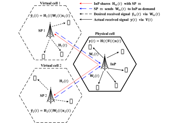
Figure 1: An illustration of MIMO virtualization in a cell with one InP and two SPs each serving its users in a virtual cell.

We adopt the spatial virtualization approach first proposed in [12], which is illustrated in Fig. 1. In the idealized case when the perfect CSI is available at each time $t$, the InP shares with SP $m$ the channel state $\mathbf{H}_{m}(t)$ between the BS and its $K_{m}$ users and allocates transmission power $P_{m}$ to the SP. Based on $\mathbf{H}_{m}(t)$, each SP $m$ designs its precoding matrix $\mathbf{W}_{m}(t)\in\mathbb{C}^{N\times K_{m}}$, subject to the transmission power limit $\|\mathbf{W}_{m}(t)\|_{F}^{2}\leq P_{m}$. The design of $\mathbf{W}_{m}(t)$ is solely based on the service needs of SP $m$’s users, without considering the existence of the other SPs sharing the same BS antennas and spectrum resource. Each SP $m$ then sends $\mathbf{W}_{m}(t)$ as its virtual precoding demand to the InP. For SP $m$, the desired received signal vector (noiseless) $\tilde{\mathbf{y}}_{m}$ (at $K_{m}$ users) is given by

$$\tilde{\mathbf{y}}_{m}(t)=\mathbf{H}_{m}(t)\mathbf{W}_{m}(t)\mathbf{x}_{m}(t)$$

where $\mathbf{x}_{m}(t)$ is the symbol vector to $K_{m}$ users. Define the desired received signal vector at all $K$ users in the network as $\tilde{\mathbf{y}}(t)\triangleq[\tilde{\mathbf{y}}_{1}^{H}(t),\dots,\tilde{\mathbf{y}}_{M}^{H}(t)]^{H}$, we have $\tilde{\mathbf{y}}(t)=\mathbf{D}(t)\mathbf{x}(t)$, where $\mathbf{D}(t)\triangleq\operatorname{blkdiag}\{\mathbf{H}_{1}(t)\mathbf{W}_{1}(t),\dots,\mathbf{H}_{M}(t)\mathbf{W}_{M}(t)\}\in\mathbb{C}^{K\times{K}}$ is the virtualization demand from all SPs, and $\mathbf{x}(t)\triangleq[\mathbf{x}_{1}^{H}(t),\dots,\mathbf{x}_{M}^{H}(t)]^{H}$ contains the symbols to all $K$ users, which are assumed to have unit power and be independent to each other, i.e., $\mathbb{E}\{\mathbf{x}(t)\mathbf{x}^{H}(t)\}=\mathbf{I},\forall{t}$.

At each time $t$, the InP designs the actual precoding matrix $\mathbf{V}(t)\triangleq[\mathbf{V}_{1}(t),\dots,\mathbf{V}_{M}(t)]\in\mathbb{C}^{N\times{K}}$, where $\mathbf{V}_{m}(t)\in\mathbb{C}^{N\times K_{m}}$ is the actual precoding matrix for SP $m$. The actual received signal vector (noiseless) $\mathbf{y}_{m}(t)$ at SP $m$’s $K_{m}$ users is given by

$$\mathbf{y}_{m}(t)=\mathbf{H}_{m}(t)\mathbf{V}_{m}(t)\mathbf{x}_{m}(t)+\sum_{i\in\mathcal{M},i\neq{m}}\mathbf{H}_{m}\mathbf{V}_{i}(t)\mathbf{x}_{i}(t),$$

where the second term is the inter-SP interference from the other SPs to SP $m$’s users. The actual received signal vector at all $K$ users is given by $\mathbf{y}(t)=[\mathbf{y}_{1}^{H}(t),\dots,\mathbf{y}_{M}^{H}(t)]^{H}=\mathbf{H}(t)\mathbf{V}(t)\mathbf{x}(t)$.

III-B Problem Formulation

For downlink MIMO WNV, the InP designs precoding matrix $\mathbf{V}(t)$ to perform MIMO virtualization. Note that while each SP $m$ designs its virtual precoding matrix $\mathbf{W}_{m}(t)$ without considering the inter-SP interference, the InP designs the actual precoding matrix $\mathbf{V}(t)$ to mitigate the inter-SP interference, in order to meet the virtualization demand $\mathbf{D}(t)$ of all SPs.

With the InP’s actual precoding matrix $\mathbf{V}(t)$ and each SP $m$’s virtual precoding matrix $\mathbf{W}_{m}(t)$, the expected deviation of the actual received signal vector at all $K$ users from the desired one is $\mathbb{E}\{\|\mathbf{y}(t)-\tilde{\mathbf{y}}(t)\|_{2}^{2}\}=\mathbb{E}\{\|\mathbf{H}(t)\mathbf{V}(t)-\mathbf{D}(t)\|_{F}^{2}\}$.

The goal at the InP is to optimize MIMO precoding to minimize the long-term time-averaged expected precoding deviation from the virtualization demands, subject to both long-term and short-term transmit power constraints. The optimization problem is formulated as follows:

$$\textbf{P1}:\quad\min_{\{\mathbf{V}(t)\}}\quad \lim_{T\to\infty}\frac{1}{T}\sum_{t=0}^{T-1}\mathbb{E}\{\|\mathbf{H}(t)\mathbf{V}(t)-\mathbf{D}(t)\|_{F}^{2}\}$$

s.t. $$\lim_{T\to\infty}\frac{1}{T}\sum_{t=0}^{T-1}\mathbb{E}\{\|\mathbf{V}(t)\|_{F}^{2}\}\leq\bar{P},$$ (2)

$$\|\mathbf{V}(t)\|_{F}^{2}\leq P_{\text{max}}$$ (3)

where $\bar{P}$ is the long-term average transmit power limit, and $P_{\text{max}}$ is the per-slot maximum transmit power limit at the BS. Both power limits are set by the InP, and we assume $\bar{P}\leq P_{\text{max}}$.

Since channel state $\mathbf{H}(t)$ is random, P1 is a stochastic optimization problem. The problem is challenging to solve, especially when the distribution of $\mathbf{H}(t)$ is unknown, especially in massive MIMO systems with a large number of antennas and users. In addition, the instantaneous channel state cannot be obtained accurately in practical systems. Typically, the InP only has an inaccurate estimate of the channel state $\hat{\mathbf{H}}(t)$ at each time $t$. With a given channel estimation quality, we assume the normalized CSI inaccuracy is bounded by a constant $\delta\geq 0$ at any time $t$, given by

$$\frac{\|\tilde{\mathbf{H}}_{m}(t)\|_{F}}{\|\mathbf{H}_{m}(t)\|_{F}}\leq\delta,\quad\forall{m}\in\mathcal{M},\quad\forall{t}$$ (4)

where $\tilde{\mathbf{H}}_{m}(t)\triangleq\mathbf{H}_{m}(t)-\hat{\mathbf{H}}_{m}(t)$ is the channel estimation error, with $\hat{\mathbf{H}}_{m}(t)$ being the estimated channel state of SP $m$’s users. By (1) and (4), the estimated channel gain is bounded by

$$\|\hat{\mathbf{H}}(t)\|_{F}\leq\|\mathbf{H}(t)\|_{F}+\|\tilde{\mathbf{H}}(t)\|_{F}\leq{B}(1+\delta),\quad\forall{t}.$$ (5)

Using the estimated channel state $\hat{\mathbf{H}}_{m}(t)$ shared by the InP at time $t$, each SP $m$ designs its virtual precoding matrix, denoted by $\hat{\mathbf{W}}_{m}(t)$. As a result, the InP receives virtualization demand $\hat{\mathbf{D}}(t)\triangleq\operatorname{blkdiag}\{\hat{\mathbf{H}}_{1}(t)\hat{\mathbf{W}}_{1}(t),\dots,\hat{\mathbf{H}}_{M}(t)\hat{\mathbf{W}}_{M}(t)\}$ from the SPs based on the imperfect CSI. Using $\hat{\mathbf{H}}(t)$ and $\hat{\mathbf{D}}(t)$, the InP then designs the actual precoding matrix, denoted by $\hat{\mathbf{V}}(t)$.

Our goal is to develop an online MIMO WNV algorithm based on $\hat{\mathbf{H}}(t)$ and $\hat{\mathbf{D}}(t)$ to find a precoding solution $\{\hat{\mathbf{V}}(t)\}$ to P1 under the unknown channel distribution $\mathbf{H}(t)$.

IV Online Single-Cell MIMO WNV Algorithm

In this section, we present a new online precoding algorithm for MIMO WNV that is developed based on the Lyapunov optimization technique. Note that the standard Lyapunov optimization relies on accurate system state [24], which is not applicable to our problem. Instead, we develop new techniques to accommodate imperfect CSI in designing the online algorithm at both the InP and the SPs.

IV-A Online Optimization Formulation

To design an online algorithm for solving P1, we introduce a virtual queue $Z(t)$ for the long-term average transmit power constraint (2) with the updating rule given by

$$Z(t+1)=\max\{Z(t)+\|\hat{\mathbf{V}}(t)\|_{F}^{2}-\bar{P},0\}.$$ (6)

Define $L(t)\triangleq\frac{1}{2}Z^{2}(t)$ as the quadratic Lyapunov function and $\Delta(t)\triangleq L(t+1)-L(t)$ as the corresponding one-slot Lyapunov drift at time $t$. By the theory of Lyapunov optimization, P1 can be converted to minimizing the objective function while stabilizing the virtual queue in (6), which can be further converted to minimizing a drift-plus-penalty (DPP) metric [24]. The DPP metric is defined as $\mathbb{E}\{\Delta(t)|Z(t)\}+U\mathbb{E}\{\hat{\rho}(t)|Z(t)\}$, where $\hat{\rho}(t)\triangleq\|\hat{\mathbf{H}}(t)\hat{\mathbf{V}}(t)-\hat{\mathbf{D}}(t)\|_{F}^{2}$ is the penalty cost representing the precoding deviation from the virtualization demands based on imperfect CSI, and $U>0$ is the relative weight. The DPP metric is a weighted sum of the expected Lyapunov drift $\Delta(t)$ and the precoding deviation $\hat{\rho}(t)$ under the current estimated channel state $\hat{\mathbf{H}}(t)$, conditioned on the current virtual queue $Z(t)$. Minimizing the DPP metric directly is still difficult due to the dynamics involved in the Lyapunov drift $\Delta(t)$. Instead, we first provide an upper bound for the DPP metric in the following lemma.

Lemma 1.

At each time $t$, for any precoding design of $\hat{\mathbf{V}}(t)$, the DPP metric has the following upper bound for all $Z(t)$ and $U>0$

$$\mathbb{E}\{\Delta(t)|Z(t)\}+U\mathbb{E}\{\hat{\rho}(t)|Z(t)\}$$

$$\leq{S}+U\mathbb{E}\left\{\hat{\rho}(t)|Z(t)\right\}+Z(t)\mathbb{E}\{\|\hat{\mathbf{V}}(t)\|_{F}^{2}-\bar{P}|Z(t)\}$$ (7)

where $S\triangleq\frac{1}{2}\max\left\{(P_{\text{max}}-\bar{P})^{2},\bar{P}^{2}\right\}$.

Proof: From the virtual queue dynamics in (6), we have

$$\Delta(t) =\frac{1}{2}\left((\max\{{Z}(t)+\|\hat{\mathbf{V}}(t)\|_{F}^{2}-\bar{P},0\})^{2}-Z^{2}(t)\right)$$

$$\leq\frac{1}{2}\left((Z(t)+\|\hat{\mathbf{V}}(t)\|_{F}^{2}-\bar{P})^{2}-Z^{2}(t)\right)$$

$$=\frac{1}{2}(\|\hat{\mathbf{V}}(t)\|_{F}^{2}-\bar{P})^{2}+Z(t)(\|\hat{\mathbf{V}}(t)\|_{F}^{2}-\bar{P}).$$ (8)

By the short-term transmit power constraint in (3), we have

$$(\|\hat{\mathbf{V}}(t)\|_{F}^{2}-\bar{P})^{2}\leq\max\{(P_{\text{max}}-\bar{P})^{2},\bar{P}^{2}\}.$$ (9)

Taking the conditional expectation at both sides of (8) for given $Z(t)$ and considering (9), we have the upper bound of the per-slot conditional expected Lyapunov drift $\Delta(t)$ given by

$$\mathbb{E}\{\Delta(t)|Z(t)\}\leq S+\mathbb{E}\left\{Z(t)(\|\hat{\mathbf{V}}(t)\|_{F}^{2}-\bar{P})|Z(t)\right\}.$$ (10)

Adding $U\mathbb{E}\{\hat{\rho}(t)|Z(t)\}$ on both sides of (10), we have (7).

Using Lemma 1, instead of directly minimizing the DPP metric, we minimize its upper bound in (7), which is no longer a function of $\Delta(t)$. Specifically, given $\hat{\mathbf{H}}(t)$ at time $t$, we consider the per-slot version of the upper bound in (7) as the optimization objective by removing the conditional expectation. By removing the constant terms, the resulting per-slot optimization problem is given by

$$\textbf{P2}:~{}\min_{\hat{\mathbf{V}}(t)}~{} U\|\hat{\mathbf{H}}(t)\hat{\mathbf{V}}(t)-\hat{\mathbf{D}}(t)\|_{F}^{2}+Z(t)\|\hat{\mathbf{V}}(t)\|_{F}^{2}$$

s.t. $$\|\hat{\mathbf{V}}(t)\|_{F}^{2}\leq P_{\text{max}}.$$ (11)

Note that P2 is a per-slot precoding optimization problem under the current estimated channel state $\hat{\mathbf{H}}(t)$ and the virtual queue $Z(t)$, subject to the per-slot maximum transmit power constraint (11). Compared with the original P1, we change the long-term time-averaged expected objective to the per-slot version of DPP metric in P2, where the long-term average transmit power constraint (2) is converted into maintaining the queue stability in $Z(t)$ as part of the DPP metric. Next, we solve P2 to obtain the optimal precoding matrix $\hat{\mathbf{V}}^{\star}(t)$ for P2 at each time $t$, and then update the virtual queue $Z(t)$ according to its queue dynamics in (6). An outline of the proposed online algorithm is given in Algorithm 1.

Algorithm 1 Outline of Online MIMO WNV Algorithm

1:  Set $U>0$ and $Z(0)=0$.

2:  At each time $t$, obtain $\hat{\mathbf{H}}(t)$ and $Z(t)$.

3:  Solve P2 for $\hat{\mathbf{V}}^{\star}(t)$ (see Section IV-B).

4:  Update $Z(t+1)=\max\{Z(t)+\|\hat{\mathbf{V}}^{\star}(t)\|_{F}^{2}-\bar{P},0\}$.

IV-B Online Precoding Solution to P2

Now we present a semi-closed-form solution to P2. Without causing any ambiguity, for notation simplicity, we omit the time index $t$ in solving P2. Note that P2 is essentially a constrained regularized least square problem. Since P2 is a convex optimization problem satisfying Slater’s condition, the strong duality holds. We solve P2 using the Karush-Kuhn-Tucker (KKT) conditions [28]. The Lagrangian for P2 is given by

$$L(\hat{\mathbf{V}},\lambda)=U\|\hat{\mathbf{H}}\hat{\mathbf{V}}-\hat{\mathbf{D}}\|_{F}^{2}+Z\|\hat{\mathbf{V}}\|_{F}^{2}+\lambda(\|\hat{\mathbf{V}}\|_{F}^{2}-P_{\text{max}})$$

$$=U(\operatorname{tr}\{\hat{\mathbf{H}}^{H}\hat{\mathbf{H}}\hat{\mathbf{V}}\hat{\mathbf{V}}^{H}\}+\operatorname{tr}\{\hat{\mathbf{D}}\hat{\mathbf{D}}^{H}\}-\operatorname{tr}\{\hat{\mathbf{H}}^{H}\hat{\mathbf{D}}\hat{\mathbf{V}}^{H}\}$$

$$\quad-\operatorname{tr}\{\hat{\mathbf{H}}\hat{\mathbf{V}}\hat{\mathbf{D}}^{H}\})+(Z+\lambda)\operatorname{tr}\{\hat{\mathbf{V}}\hat{\mathbf{V}}^{H}\}-\lambda{P}_{\text{max}}$$

where $\lambda$ is the Lagrange multiplier associated with the maximum power constraint (11). The gradient of $L(\hat{\mathbf{V}},\lambda)$ w.r.t. $\mathbf{\hat{V}}^{*}$ is given by

$$\nabla_{\mathbf{\hat{V}}^{*}}L(\hat{\mathbf{V}},\lambda)=U(\hat{\mathbf{H}}^{H}\hat{\mathbf{H}}\hat{\mathbf{V}}-\hat{\mathbf{H}}^{H}\hat{\mathbf{D}})+(Z+\lambda)\hat{\mathbf{V}}$$ (12)

where the following fact is used: $\nabla_{\mathbf{B}^{*}}\operatorname{tr}\{\mathbf{AB}^{H}\}=\mathbf{A}$ and $\nabla_{\mathbf{B}^{*}}\operatorname{tr}\{\mathbf{AB}\}=\mathbf{0}$ [29]. The optimal solution to P2 can be obtained by solving the KKT conditions, given by

$$\left(\hat{\mathbf{H}}^{H}\hat{\mathbf{H}}+\frac{Z+\lambda^{\star}}{U}\mathbf{I}\right)\hat{\mathbf{V}}^{\star} =\hat{\mathbf{H}}^{H}\hat{\mathbf{D}},$$ (13)

$$\|\hat{\mathbf{V}}^{\star}\|_{F}^{2}-P_{\text{max}} \leq 0,$$ (14)

$$\lambda^{\star} \geq{0},$$ (15)

$$\lambda^{\star}(\|\hat{\mathbf{V}}^{\star}\|_{F}^{2}-P_{\text{max}}) =0$$ (16)

where (13) is obtained by setting $\nabla_{\mathbf{\hat{V}}^{*}}L(\hat{\mathbf{V}},\lambda)$ in (12) to $\mathbf{0}$. Note that, by (6), the virtual queue is nonnegative, i.e., $Z\geq 0$. Thus, we derive the optimal solution in the following two cases.

IV-B1 $Z+\lambda^{\star}>0$

From (13) and $\hat{\mathbf{H}}^{H}\hat{\mathbf{H}}+\frac{Z+\lambda^{\star}}{U}\mathbf{I}\succ\mathbf{0}$, we have

$$\hat{\mathbf{V}}^{\star}=\left(\hat{\mathbf{H}}^{H}\hat{\mathbf{H}}+\frac{Z+\lambda^{\star}}{U}\mathbf{I}\right)^{-1}\hat{\mathbf{H}}^{H}\hat{\mathbf{D}}.$$ (17)

Depending on $Z$, we determine $\lambda^{\star}$ in (17) in two subcases: 1.1) If $Z>0$: By (14) and (16), we conclude that if $\|(\hat{\mathbf{H}}^{H}\hat{\mathbf{H}}+\frac{Z}{U}\mathbf{I})^{-1}\hat{\mathbf{H}}^{H}\hat{\mathbf{D}}\|_{F}^{2}\leq{P}_{\text{max}}$, then $\lambda^{\star}=0$; Otherwise, we have $\lambda^{\star}>0$ such that $\|(\hat{\mathbf{H}}^{H}\hat{\mathbf{H}}+\frac{Z+\lambda^{\star}}{U}\mathbf{I})^{-1}\hat{\mathbf{H}}^{H}\hat{\mathbf{D}}\|_{F}^{2}=P_{\text{max}}$. 1.2) If $Z=0$: In this case, $\lambda^{\star}>0$. By (16), the value of $\lambda^{\star}$ satisfies $\|(\hat{\mathbf{H}}^{H}\hat{\mathbf{H}}+\frac{\lambda^{\star}}{U}\mathbf{I})^{-1}\hat{\mathbf{H}}^{H}\hat{\mathbf{D}}\|_{F}^{2}=P_{\text{max}}$.

IV-B2 $Z=\lambda^{\star}=0$

From (13), the optimal solution must satisfy

$$\hat{\mathbf{H}}^{H}\hat{\mathbf{H}}\hat{\mathbf{V}}^{\star}=\hat{\mathbf{H}}^{H}\hat{\mathbf{D}}.$$ (18)

We analyze (18) in two subcases: 2.1) If $K<N$: $\hat{\mathbf{H}}^{H}\hat{\mathbf{H}}\in\mathbb{C}^{N\times{N}}$ is a rank-deficient matrix, and thus there are infinitely many solutions to $\hat{\mathbf{V}}^{\star}$. We choose $\hat{\mathbf{V}}^{\star}$ that minimizes $\|\hat{\mathbf{V}}^{\star}\|_{F}^{2}$ subject to (18). This problem is an under-determined least square problem with a closed-form solution:

$$\hat{\mathbf{V}}^{\star}=\hat{\mathbf{H}}^{H}\left(\hat{\mathbf{H}}\hat{\mathbf{H}}^{H}\right)^{-1}\hat{\mathbf{D}}.$$ (19)

Substitute the above expression of $\hat{\mathbf{V}}^{\star}$ into the power constraint in (14). If $\|\hat{\mathbf{H}}^{H}(\hat{\mathbf{H}}\hat{\mathbf{H}}^{H})^{-1}\hat{\mathbf{D}}\|_{F}^{2}\leq{P}_{\text{max}}$, then $\hat{\mathbf{V}}^{\star}$ in (19) is the optimal solution. Otherwise, see the discussion in the next paragraph. 2.2) If $K\geq N$: $\hat{\mathbf{H}}^{H}\hat{\mathbf{H}}\!\in\!\mathbb{C}^{N\times{N}}$ is full rank, and we have a unique solution:

$$\hat{\mathbf{V}}^{\star}=\left(\hat{\mathbf{H}}^{H}\hat{\mathbf{H}}\right)^{-1}\hat{\mathbf{H}}^{H}\hat{\mathbf{D}}.$$ (20)

Again, substituting $\hat{\mathbf{V}}^{\star}$ in (20) into (14), if $\|(\hat{\mathbf{H}}^{H}\hat{\mathbf{H}})^{-1}\hat{\mathbf{H}}^{H}\hat{\mathbf{D}}\|_{F}^{2}\leq{P}_{\text{max}}$, then $\hat{\mathbf{V}}^{\star}$ in (20) is the optimal solution.

Note that, for both subcases 2.1) and 2.2), if $\hat{\mathbf{V}}^{\star}$ in (19) or (20) cannot satisfy the power constraint in (14), it means that the condition in Case 2) does not hold at optimality, and we have $\lambda^{\star}>0$, i.e., the optimal solution is given by (17).

From the above discussion, if $\lambda^{\star}=0$ at the optimality, we have a closed-form solution for $\hat{\mathbf{V}}^{\star}$ in (19) or (20). Otherwise, we have a semi-closed-form solution for $\hat{\mathbf{V}}^{\star}$ in (17), where $\lambda^{\star}>0$ can be obtained through the bi-section search to ensure the transmit power meets $P_{\text{max}}$ in (14). The computational complexity for calculating $\hat{\mathbf{V}}^{\star}$ is dominated by the matrix inversion, and thus is in the order of $\mathcal{O}(\min(N,K)^{3})$.

V Performance Bounds for Single-Cell Case

Different from existing MIMO precoding designs for non-virtualized networks such as in [27], for the MIMO WNV design, the impact of imperfect CSI on the system is two-fold at both the InP and the SPs. This brings some unique challenges in analyzing the performance of the proposed online algorithm. In this section, we develop new techniques to derive the performance bounds for our online algorithm.

First, we show in the following lemma that by Algorithm 1, the virtual queue $Z(t)$ is upper bounded at each time $t$.

Lemma 2.

By Algorithm 1, $Z(t)$ satisfies

$$Z(t)\leq UB^{2}(1+\delta)^{2}\xi+P_{\text{max}}-\bar{P},\quad\forall{t}$$ (21)

where $\xi\triangleq\sqrt{\frac{N}{\bar{P}}\sum_{m\in\mathcal{M}}P_{m}}$.

Proof: We first omit time index $t$ for simplicity. Let $\hat{\mathbf{H}}^{H}\hat{\mathbf{H}}=\hat{\mathbf{U}}\hat{\boldsymbol{\Sigma}}\hat{\mathbf{U}}^{H}$, where $\hat{\mathbf{U}}$ is an unitary matrix, and $\hat{\boldsymbol{\Sigma}}=\operatorname{diag}(\hat{\sigma}_{1},\dots,\hat{\sigma}_{N})$. It follows that $\hat{\mathbf{H}}^{H}\hat{\mathbf{H}}+\frac{Z+\lambda^{\star}}{U}\mathbf{I}=\hat{\mathbf{U}}\hat{\boldsymbol{\Phi}}\hat{\mathbf{U}}^{H}$, where $\hat{\boldsymbol{\Phi}}=\operatorname{diag}(\hat{\phi}_{1},\dots,\hat{\phi}_{N})$ and $\hat{\phi}_{n}=\hat{\sigma}_{n}+\frac{Z+\lambda^{\star}}{U},\forall{n}\in\mathcal{N}$. If $Z>0$, $\hat{\mathbf{V}}^{\star}$ is given in (17), and we have

$$\|\hat{\mathbf{V}}^{\star}\|_{F} \leq\left\|\hat{\mathbf{U}}\hat{\boldsymbol{\Phi}}^{-1}\hat{\mathbf{U}}^{H}\right\|_{F}\|\hat{\mathbf{H}}\|_{F}\|\hat{\mathbf{D}}\|_{F}\stackrel{{\scriptstyle(a)}}{{\leq}}\frac{U}{Z}\sqrt{N}\|\hat{\mathbf{H}}\|_{F}\|\hat{\mathbf{D}}\|_{F}$$

$$\stackrel{{\scriptstyle(b)}}{{\leq}}\frac{U}{Z}B^{2}(1+\delta)^{2}\sqrt{N\sum_{m\in\mathcal{M}}P_{m}}.\!\!$$ (22)

Inequality $(a)$ follows from $\|\hat{\mathbf{U}}\hat{\boldsymbol{\Phi}}^{-1}\hat{\mathbf{U}}^{H}\|_{F}^{2}=\operatorname{tr}\{\hat{\boldsymbol{\Phi}}^{-2}\}=\sum_{n\in\mathcal{N}}\hat{\phi}_{n}^{-2}$. Since $\hat{\sigma}_{n}\geq 0,\forall{n}\in\mathcal{N}$, $\lambda^{\star}\geq 0$, and $Z>0$, it follows that $\hat{\phi}_{n}^{-2}\leq\frac{U^{2}}{Z^{2}},\forall{n}\in\mathcal{N}$, and therefore $\|\hat{\mathbf{U}}\hat{\boldsymbol{\Phi}}^{-1}\hat{\mathbf{U}}^{H}\|_{F}^{2}\leq{N}\frac{U^{2}}{Z^{2}}$. Inequality $(b)$ follows from (5) and by the definition of $\hat{\mathbf{D}}$

$$\!\!\|\hat{\mathbf{D}}\|_{F}^{2}\leq\!\!\sum_{m\in\mathcal{M}}\|\hat{\mathbf{H}}_{m}\|_{F}^{2}\|\hat{\mathbf{W}}_{m}\|_{F}^{2}\leq{B^{2}}(1+\delta)^{2}\sum_{m\in\mathcal{M}}P_{m}.\!\!$$ (23)

From (22), a sufficient condition to ensure $\|\hat{\mathbf{V}}^{\star}\|_{F}^{2}\leq\bar{P}$ is that the RHS of (22) is less than $\sqrt{\bar{P}}$, which means $Z\geq UB^{2}(1+\delta)^{2}\sqrt{\frac{N}{\bar{P}}\sum_{m\in\mathcal{M}}P_{m}}$. Consider time index $t$. If the condition holds, $\|\hat{\mathbf{V}}^{\star}(t)\|_{F}^{2}\leq\bar{P}$, the virtual queue in (6) decreases, i.e., $Z(t+1)\leq Z(t)$. Otherwise, the maximum increment of the virtual queue is $P_{\text{max}}-\bar{P}$, i.e., $Z(t+1)\leq Z(t)+P_{\text{max}}-\bar{P}$. Thus, we have the upper bound of $Z(t)$ in (21) at any time $t\geq{0}$.

Note that Algorithm 1 and the upper bound on the virtual queue in Lemma 2 are applicable to any precoding schemes adopted by the SPs. In the following, we consider two common precoding schemes: maximum ratio transmission (MRT) and zero forcing (ZF). We assume $M_{\text{\tiny MRT}}$ SPs adopt MRT precoding and the rest of SPs adopt ZF precoding. We point out that although the following analysis focuses on the two precoding schemes, the similar analysis can be extended to other precoding schemes as well.

Let $\mathcal{M}_{\text{\tiny MRT}}=\{1,\dots,M_{\text{\tiny MRT}}\}$ be the set of SPs that adopt MRT precoding, with the MRT precoding matrix given by

$$\hat{\mathbf{W}}_{m}^{\text{\tiny MRT}}(t)=\sqrt{P_{m}}\frac{\hat{\mathbf{H}}_{m}^{H}(t)}{\|\hat{\mathbf{H}}_{m}(t)\|_{F}}.$$ (24)

Each SP $m\in\mathcal{M}\backslash\mathcal{M}_{\text{\tiny MRT}}$ adopts ZF precoding to null the intra-SP interference. We assume $K_{m}\leq N$ to use ZF precoding. The ZF precoding matrix is given by

$$\hat{\mathbf{W}}_{m}^{\text{\tiny ZF}}(t)=\sqrt{P_{m}}\frac{\hat{\mathbf{H}}_{m}^{H}(t)[\hat{\mathbf{H}}_{m}(t)\hat{\mathbf{H}}_{m}^{H}(t)]^{-1}}{\sqrt{\operatorname{tr}\{[\hat{\mathbf{H}}_{m}(t)\hat{\mathbf{H}}_{m}^{H}(t)]^{-1}\}}}.$$ (25)

With the two precoding matrices in (24) and (25), we first quantify the impact of inaccurate CSI on the SPs’ virtualization demands by providing an upper bound on the deviation between the accurate and inaccurate virtualization demands $\|\mathbf{D}(t)-\hat{\mathbf{D}}(t)\|_{F}$, for given CSI inaccuracy $\delta$ in (4). This effect of $\delta$ on the precoding performance is unique to the MIMO WNV system and has not been studied before.

Let $\omega_{m,1}(t),\dots,\omega_{m,K_{m}}(t)$ be the eigenvalues of $\hat{\mathbf{H}}_{m}\hat{\mathbf{H}}_{m}^{H}$, and similarly, $\hat{\omega}_{m,1}(t),\dots,\hat{\omega}_{m,K_{m}}(t)$ the eigenvalues of $\hat{\mathbf{H}}_{m}(t)\hat{\mathbf{H}}_{m}^{H}(t)$. Define $\hat{B}_{m}^{\text{\tiny min}}\triangleq\min\{\|\hat{\mathbf{H}}_{m}(t)\|_{F}:\forall{t}\}$, $\hat{\omega}_{m}^{\text{\tiny min}}\triangleq\min\{\hat{\omega}_{m,i}(t):\forall{i}\in\mathcal{K}_{m},\forall{t}\}$, and $\omega_{m}^{\text{\tiny min}}\triangleq\min\{\omega_{m,i}(t):\forall{i}\in\mathcal{K}_{m},\forall{t}\}$, which respectively represent the minimum channel gain of $\hat{\mathbf{H}}_{m}(t)$, the minimum energy in the eigen-directions of $\hat{\mathbf{H}}_{m}(t)$, and that of $\mathbf{H}_{m}(t)$. We have the following lemma.

Lemma 3.

At each time $t$, the following hold:

$$\|\mathbf{D}(t)\|_{F} \leq\zeta B,$$ (26)

$$\|\hat{\mathbf{D}}(t)\|_{F} \leq\zeta B(1+\delta),$$ (27)

$$\|\mathbf{D}(t)-\hat{\mathbf{D}}(t)\|_{F} \leq\eta{B}\delta,$$ (28)

where

$\eta\!\triangleq\!\!\sqrt{\displaystyle\!\sum_{m\in\mathcal{M}_{\text{\tiny MRT}}}\!\!\left(\!1\!+\!\frac{(2\!+\!\delta)B}{\hat{B}_{m}^{\text{\tiny min}}}\!\right)^{\!2}\!\!\!P_{m}\!+\!\!\!\!\sum_{m\in\mathcal{M}\backslash\mathcal{M}_{\text{\tiny MRT}}}\!\!\left(\!\frac{B^{4}(1\!+\!\delta)^{2}}{K_{m}\hat{\omega}_{m}^{\text{\tiny min}}\omega_{m}^{\text{\tiny min}}}\!\!\right)^{\!2}\!\!\!P_{m}}$, and $\zeta\triangleq\!\sqrt{\sum_{m\in\mathcal{M}}P_{m}}$.

Proof: The proofs of (26) and (27) follow from (23). To prove (28), we omit time index $t$ for notation simplicity. By the definition of $\mathbf{D}$ and $\hat{\mathbf{D}}$, we have

$$\|\mathbf{D}-\hat{\mathbf{D}}\|_{F}^{2}=\sum_{m\in\mathcal{M}}\|\mathbf{H}_{m}\mathbf{W}_{m}-\hat{\mathbf{H}}_{m}\hat{\mathbf{W}}_{m}\|_{F}^{2}.$$ (29)

Using the MRT precoding in (24) for $m\in\mathcal{M}_{\text{\tiny MRT}}$ we have

$$\|\mathbf{H}_{m}\mathbf{W}_{m}^{\text{\tiny MRT}}-\hat{\mathbf{H}}_{m}\hat{\mathbf{W}}_{m}^{\text{\tiny MRT}}\|_{F}$$

$$=\sqrt{P_{m}}\left\|\frac{\mathbf{H}_{m}\mathbf{H}_{m}^{H}}{\|\mathbf{H}_{m}\|_{F}}-\frac{\hat{\mathbf{H}}_{m}\hat{\mathbf{H}}_{m}^{H}}{\|\hat{\mathbf{H}}_{m}\|_{F}}\right\|_{F}$$

$$=\sqrt{P_{m}}\left\|\frac{\mathbf{H}_{m}\mathbf{H}_{m}^{H}}{\|\mathbf{H}_{m}\|_{F}}-\frac{(\mathbf{H}_{m}-\tilde{\mathbf{H}}_{m})(\mathbf{H}_{m}^{H}-\tilde{\mathbf{H}}_{m}^{H})}{\|\mathbf{H}_{m}-\tilde{\mathbf{H}}_{m}\|_{F}}\right\|_{F}$$

$$=\sqrt{P_{m}}\left\|\left(\frac{\mathbf{H}_{m}\mathbf{H}_{m}^{H}}{\|\mathbf{H}_{m}\|_{F}}-\frac{\mathbf{H}_{m}\mathbf{H}_{m}^{H}}{\|\mathbf{H}_{m}-\tilde{\mathbf{H}}_{m}\|_{F}}\right)\right.$$

$$\quad\left.-\frac{\tilde{\mathbf{H}}_{m}\tilde{\mathbf{H}}_{m}^{H}-2\Re\{\tilde{\mathbf{H}}_{m}\mathbf{H}_{m}^{H}\}}{\|\mathbf{H}_{m}-\tilde{\mathbf{H}}_{m}\|_{F}}\right\|_{F}$$

$$\leq\sqrt{P_{m}}\left[\frac{\|\mathbf{H}_{m}\mathbf{H}_{m}^{H}\|_{F}}{\|\mathbf{H}_{m}\|_{F}}\left(1-\frac{\|\mathbf{H}_{m}\|_{F}}{\|\mathbf{H}_{m}-\tilde{\mathbf{H}}_{m}\|_{F}}\right)\right.$$

$$\quad\left.+\frac{\|\tilde{\mathbf{H}}_{m}\tilde{\mathbf{H}}_{m}^{H}-2\Re\{\tilde{\mathbf{H}}_{m}\mathbf{H}_{m}^{H}\}\|_{F}}{\|\mathbf{H}_{m}-\tilde{\mathbf{H}}_{m}\|_{F}}\right]$$

$$\stackrel{{\scriptstyle(a)}}{{\leq}}\sqrt{P_{m}}\left(B\delta+\frac{\|\tilde{\mathbf{H}}_{m}\tilde{\mathbf{H}}_{m}^{H}-2\Re\{\tilde{\mathbf{H}}_{m}\mathbf{H}_{m}^{H}\}\|_{F}}{\|\mathbf{H}_{m}-\tilde{\mathbf{H}}_{m}\|_{F}}\right)$$

$$\stackrel{{\scriptstyle(b)}}{{\leq}}\sqrt{P_{m}}B\delta\!\left(\!\!1\!+\!\frac{(2\!+\!\delta)B}{\|\hat{\mathbf{H}}_{m}\|_{F}}\!\!\right)\!\leq\!\sqrt{P_{m}}B\delta\!\left(\!\!1\!+\!\frac{(2\!+\!\delta)B}{\hat{B}_{m}^{\text{\tiny min}}}\!\!\right)\!$$ (30)

where $(a)$ is because

$$\frac{\|\mathbf{H}_{m}\mathbf{H}_{m}^{H}\|_{F}}{\|\mathbf{H}_{m}\|_{F}}\left(\!1\!-\!\frac{\|\mathbf{H}_{m}\|_{F}}{\|\mathbf{H}_{m}\!-\!\tilde{\mathbf{H}}_{m}\|_{F}}\!\right)$$

$$\leq\frac{\|\mathbf{H}_{m}\|_{F}^{2}}{\|\mathbf{H}_{m}\|_{F}}\left(1-\frac{\|\mathbf{H}_{m}\|_{F}}{\|\tilde{\mathbf{H}}_{m}\|_{F}\!+\!\|\mathbf{H}_{m}\|_{F}}\right)\!\leq{\!B}\!\left(\!1\!-\!\frac{1}{1\!+\!\delta}\!\right)\!\leq\!B\delta,$$

in which we use $\|\mathbf{H}_{m}\|_{F}\!\leq\!{B}$ and $\|\tilde{\mathbf{H}}_{m}\|_{F}\!\leq\!{B\delta}$ from (1) and (4), respectively; and $(b)$ is because

$$\|\tilde{\mathbf{H}}_{m}\tilde{\mathbf{H}}_{m}^{H}-2\Re\{\tilde{\mathbf{H}}_{m}\mathbf{H}_{m}^{H}\}\|_{F}\leq\|\tilde{\mathbf{H}}_{m}\tilde{\mathbf{H}}_{m}^{H}\|_{F}+2\|\tilde{\mathbf{H}}_{m}\mathbf{H}_{m}^{H}\|_{F}$$

$$\leq\!\|\tilde{\mathbf{H}}_{m}\|_{F}^{2}\!+\!2\|\tilde{\mathbf{H}}_{m}\|_{F}\|\mathbf{H}_{m}\|_{F}\leq\!B^{2}\delta^{2}\!+\!2B^{2}\delta\leq\!(2\!+\!\delta)B^{2}\delta.$$

With ZF precoding in (25) for $m\in\mathcal{M}\backslash\mathcal{M}_{\text{\tiny MRT}}$, we have

$$\|\mathbf{H}_{m}\mathbf{W}_{m}^{\text{\tiny ZF}}-\hat{\mathbf{H}}_{m}\hat{\mathbf{W}}_{m}^{\text{\tiny ZF}}\|_{F}$$

$$=\sqrt{P_{m}}\left\|\frac{\mathbf{I}}{\sqrt{\operatorname{tr}\{(\mathbf{H}_{m}\mathbf{H}_{m}^{H})^{-1}\}}}-\frac{\mathbf{I}}{\sqrt{\operatorname{tr}\{(\hat{\mathbf{H}}_{m}\hat{\mathbf{H}}_{m}^{H})^{-1}\}}}\right\|_{F}$$

$$\stackrel{{\scriptstyle(a)}}{{\leq}}\!\sqrt{P_{m}K_{m}}\frac{\left|\sqrt{\sum_{i\in\mathcal{K}_{m}}\!\hat{\omega}_{m,i}^{-1}}-\!\sqrt{\sum_{i\in\mathcal{K}_{m}}\!\omega_{m,i}^{-1}}\right|}{\frac{K_{m}}{B^{2}(1+\delta)}}$$

$$=\!\sqrt{\frac{P_{m}}{K_{m}}}B^{2}(1\!+\!\delta)\frac{\left|\sum_{i\in\mathcal{K}_{m}}\left(\hat{\omega}_{m,i}^{-1}-\omega_{m,i}^{-1}\right)\right|}{\sqrt{\sum_{i\in\mathcal{K}_{m}}\!\hat{\omega}_{m,i}^{-1}}+\sqrt{\sum_{i\in\mathcal{K}_{m}}\!\omega_{m,i}^{-1}}}$$

$$\stackrel{{\scriptstyle(b)}}{{\leq}}\!\sqrt{\frac{P_{m}}{K_{m}}}B^{2}(1+\delta)\frac{B^{2}(2+\delta)\delta}{\hat{\omega}_{m}^{\text{\tiny min}}\omega_{m}^{\text{\tiny min}}\frac{(2+\delta)\sqrt{K_{m}}}{B(1+\delta)}}\leq\frac{\sqrt{P_{m}}B^{5}(1+\delta)^{2}\delta}{K_{m}\hat{\omega}_{m}^{\text{\tiny min}}\omega_{m}^{\text{\tiny min}}}$$ (31)

where $(a)$ follows from $\hat{\omega}_{m,i}\leq\|\hat{\mathbf{H}}_{m}\|_{F}^{2},\forall{i}\in\mathcal{K}_{m}$, and $\|\hat{\mathbf{H}}\|_{F}\leq{B(1+\delta)}$ in (5), such that $\operatorname{tr}\{(\hat{\mathbf{H}}_{m}\hat{\mathbf{H}}_{m}^{H})^{-1}\}=\sum_{i\in\mathcal{K}_{m}}\hat{\omega}_{m,i}^{-1}\geq\frac{K_{m}}{B^{2}(1+\delta)^{2}}$, and similarly $\operatorname{tr}\{(\mathbf{H}_{m}\mathbf{H}_{m}^{H})^{-1}\}=\sum_{i\in\mathcal{K}_{m}}\omega_{m,i}^{-1}\geq\frac{K_{m}}{B^{2}}$ for accurate CSI; $(b)$ is because

$$\sqrt{\sum_{i\in\mathcal{K}_{m}}\hat{\omega}_{m,i}^{-1}}+\!\sqrt{\sum_{i\in\mathcal{K}_{m}}\omega_{m,i}^{-1}}\geq\sqrt{\frac{K_{m}}{\|\hat{\mathbf{H}}_{m}\|_{F}^{2}}}+\sqrt{\frac{K_{m}}{\|\mathbf{H}_{m}\|_{F}^{2}}}$$

$$\geq\sqrt{\frac{K_{m}}{B^{2}(1+\delta)^{2}}}+\sqrt{\frac{K_{m}}{B^{2}}}=\frac{(2+\delta)\sqrt{K_{m}}}{B(1+\delta)},$$

$$\left|\sum_{i\in\mathcal{K}_{m}}\left(\hat{\omega}_{m,i}^{-1}-\omega_{m,i}^{-1}\right)\right|$$

$$\leq\frac{\left|\sum_{i\in\mathcal{K}_{m}}\left(\omega_{m,i}-\hat{\omega}_{m,i}\right)\right|}{\hat{\omega}_{m}^{\text{\tiny min}}\omega_{m}^{\text{\tiny min}}}=\frac{\left|\|\mathbf{H}_{m}\|_{F}^{2}-\|\hat{\mathbf{H}}_{m}\|_{F}^{2}\right|}{\hat{\omega}_{m}^{\text{\tiny min}}\omega_{m}^{\text{\tiny min}}}$$

$$=\frac{(\|\mathbf{H}_{m}\|_{F}+\|\hat{\mathbf{H}}_{m}\|_{F})\left|\|\mathbf{H}_{m}\|_{F}-\|\hat{\mathbf{H}}_{m}\|_{F}\right|}{\hat{\omega}_{m}^{\text{\tiny min}}\omega_{m}^{\text{\tiny min}}}\leq\frac{B^{2}(2+\delta)\delta}{\hat{\omega}_{m}^{\text{\tiny min}}\omega_{m}^{\text{\tiny min}}}$$

where we apply $\|\mathbf{\mathbf{H}}_{m}\|_{F}\leq{B}$, $\|\hat{\mathbf{H}}_{m}\|_{F}\leq{B}(1+\delta)$, and $|\|\mathbf{H}_{m}\|_{F}-\|\hat{\mathbf{H}}_{m}\|_{F}|\leq\|\mathbf{H}_{m}-\hat{\mathbf{H}}_{m}\|_{F}\leq{B}\delta$ resulting from (1) and (4) to the last step.

Applying inequalities (30) and (31) to the respective terms in the RHS of (29) yields (28).

For channel state $\mathbf{H}(t)$ being i.i.d. over time, there exists a stationary randomized optimal precoding solution $\mathbf{V}^{\text{\tiny opt}}(t)$ to P1, which depends only on the (unknown) distribution of $\mathbf{H}(t)$ and achieves the minimum objective value of P1, defined in Theorem 6 [24]. Define $\phi(\mathbf{H}(t),\mathbf{V}(t),\mathbf{D}(t))\triangleq{U}\|\mathbf{H}(t)\mathbf{V}(t)-\mathbf{D}(t)\|_{F}^{2}+Z(t)\|\mathbf{V}(t)\|_{F}^{2}$. Note that $\phi(\hat{\mathbf{H}}(t),\hat{\mathbf{V}}(t),\hat{\mathbf{D}}(t))$ is the objective function in P2. Using Lemma 3, for a given CSI inaccuracy $\delta$ in (4), we now bound $\phi(\mathbf{H}(t),\hat{\mathbf{V}}^{\star}(t),\mathbf{D}(t))-\phi(\mathbf{H}(t),\mathbf{V}^{\text{\tiny opt}}(t),\mathbf{\mathbf{D}}(t))$, where the first term is the objective value of P2 under the optimal solution $\hat{\mathbf{V}}^{\star}(t)$ to P2 obtained based on the inaccurate channel state $\hat{\mathbf{H}}(t)$, and the second term is the objective value of P2 by using the optimal solution $\mathbf{V}^{\text{\tiny opt}}(t)$ to P1 obtained based on the accurate channel state $\mathbf{H}(t)$.

Lemma 4.

At each time $t$, the following holds

$$\phi(\mathbf{H}(t),\hat{\mathbf{V}}^{\star}(t),\mathbf{D}(t))-\phi(\mathbf{H}(t),\mathbf{V}^{\text{\tiny opt}}(t),\mathbf{D}(t))\leq{U}\varphi$$ (32)

where

$$\varphi\triangleq 2\!\left[(2\!+\!\delta)(P_{\text{max}}\!+\!\zeta\eta)\!+\!2(\zeta(1\!+\!\delta)\!+\!\eta)\sqrt{\!P_{\text{max}}}\right]\!B^{2}\delta\!=\!O(\delta).$$

Proof: We omit time index $t$ in the proof. The proof of (32) consists of five steps as follows.

Step 1: Note that $\phi(\mathbf{H},\hat{\mathbf{V}}^{\star},\mathbf{D})$ is convex with respect to (w.r.t.) $\mathbf{D}$. By the first-order condition for a convex function [30], we have

$$\phi(\mathbf{H},\hat{\mathbf{V}}^{\star},\mathbf{D})-\phi(\mathbf{H},\hat{\mathbf{V}}^{\star},\hat{\mathbf{D}})$$

$$\leq-2\Re\{\operatorname{tr}\{\nabla_{\mathbf{\mathbf{D}}^{*}}\phi(\mathbf{H},\hat{\mathbf{V}}^{\star},\mathbf{D})^{H}(\hat{\mathbf{D}}-\mathbf{D})\}\}$$

$$\stackrel{{\scriptstyle(a)}}{{=}}2U\Re\{\operatorname{tr}\{(\mathbf{H}\hat{\mathbf{V}}^{\star}-\mathbf{D})^{H}(\hat{\mathbf{D}}-\mathbf{D})\}\}$$

$$\leq 2U|\operatorname{tr}\{(\mathbf{H}\hat{\mathbf{V}}^{\star}-\mathbf{D})^{H}(\hat{\mathbf{D}}-\mathbf{D})\}|$$

$$\leq 2U(\|\mathbf{H}\|_{F}\|\hat{\mathbf{V}}^{\star}\|_{F}+\|\mathbf{D}\|_{F})\|\hat{\mathbf{D}}-\mathbf{D}\|_{F}$$

$$\stackrel{{\scriptstyle(b)}}{{\leq}}{2}U(\sqrt{P_{\text{max}}}+\zeta)\eta{B}^{2}\delta$$

where $(a)$ follows from $\nabla_{\mathbf{D}^{*}}\phi(\mathbf{H},\hat{\mathbf{V}}^{\star},\mathbf{\mathbf{D}})=-U(\mathbf{H}\hat{\mathbf{V}}^{\star}-\mathbf{D})$, and $(b)$ follow from (1), (11), (26), and (28).

Step 2: By the first-order condition for the convex function $\phi(\mathbf{H},\hat{\mathbf{V}}^{\star},\hat{\mathbf{D}})$ w.r.t. $\mathbf{H}$, we have

$$\phi(\mathbf{H},\hat{\mathbf{V}}^{\star},\hat{\mathbf{D}})-\phi(\hat{\mathbf{H}},\hat{\mathbf{V}}^{\star},\hat{\mathbf{D}})$$

$$\leq-{2}\Re\{\operatorname{tr}\{\nabla_{\mathbf{H}^{*}}\phi(\mathbf{H},\hat{\mathbf{V}}^{\star},\hat{\mathbf{D}})^{H}(\hat{\mathbf{H}}-\mathbf{H})\}\}$$

$$\stackrel{{\scriptstyle(a)}}{{=}}2U\Re\{\operatorname{tr}\{(\mathbf{H}\hat{\mathbf{V}}^{\star}\hat{\mathbf{V}}^{\star{H}}-\hat{\mathbf{D}}\hat{\mathbf{V}}^{\star{H}})^{H}(\mathbf{H}-\hat{\mathbf{H}})\}\}$$

$$\leq{2U}|\operatorname{tr}\{(\mathbf{H}\hat{\mathbf{V}}^{\star}\hat{\mathbf{V}}^{\star{H}}-\hat{\mathbf{D}}\hat{\mathbf{V}}^{\star{H}})^{H}(\mathbf{H}-\hat{\mathbf{H}})\}|$$

$$\leq 2U(\|\mathbf{H}\|_{F}\|\mathbf{\hat{\mathbf{V}}}^{\star}\|_{F}+\|\hat{\mathbf{D}}\|_{F})\|\hat{\mathbf{V}}^{\star}\|_{F}\|\mathbf{H}-\hat{\mathbf{H}}\|_{F}$$

$$\stackrel{{\scriptstyle(b)}}{{\leq}}2U\left[P_{\text{max}}+\zeta(1+\delta)\sqrt{P_{\text{max}}}\right]B^{2}\delta$$

where $(a)$ follows from $\nabla_{\mathbf{H}^{*}}\phi(\mathbf{H},\hat{\mathbf{V}}^{\star},\hat{\mathbf{D}})=U(\mathbf{H}\hat{\mathbf{V}}^{\star}\hat{\mathbf{V}}^{\star{H}}-\hat{\mathbf{D}}\hat{\mathbf{V}}^{\star{H}})$, and $(b)$ follows from (1), (4), (11), and (27).

Step 3: In Algorithm 1, $\hat{\mathbf{V}}^{\star}$ is the optimal precoder that minimizes the objective $\phi(\hat{\mathbf{H}},\hat{\mathbf{V}},\hat{\mathbf{D}})$ of P2 over all precoding policies including $\mathbf{V}^{\text{\tiny opt}}$. It follows that

$$\phi(\hat{\mathbf{H}},\hat{\mathbf{V}}^{\star},\hat{\mathbf{D}})-\phi(\hat{\mathbf{H}},\mathbf{V}^{\text{\tiny opt}},\hat{\mathbf{D}})\leq 0.$$

Step 4: Similarly to Step 2, we have

$$\phi(\hat{\mathbf{H}},\mathbf{V}^{\text{\tiny opt}},\hat{\mathbf{D}})-\phi(\mathbf{H},\mathbf{V}^{\text{\tiny opt}},\hat{\mathbf{D}})$$

$$\leq 2U(P_{\text{max}}+\zeta\sqrt{P_{\text{max}}})(1+\delta)B^{2}\delta.$$

Step 5: Similarly to Step 1, we have

$$\phi(\mathbf{H},\mathbf{V}^{\text{\tiny opt}},\hat{\mathbf{D}})-\phi(\mathbf{H},\mathbf{V}^{\text{\tiny opt}},\mathbf{D})$$

$$\leq{2U}\left[\sqrt{P_{\text{max}}}+\zeta(1+\delta)\right]\eta{B}^{2}\delta.$$

Summing over Steps 1-5, yields (32).

Remark 1.

We point out that, different from [21], our proof in Lemma 4 explicitly considers the two-fold impact of CSI inaccuracy on both InP and SPs under MIMO WNV.

Based on Lemma 4, we next show that with the optimal $\hat{\mathbf{V}}(t)$ to P2, the expected DPP metric averaged over the virtual queue $Z(t)$ under the accurate channel state $\mathbf{H}(t)$ is upper bounded.

Lemma 5.

At each time $t$, we have

$$\mathbb{E}\{\Delta(t)\}+U\mathbb{E}\{\|\mathbf{H}(t)\hat{\mathbf{V}}^{\star}(t)-\mathbf{D}(t)\|_{F}^{2}\}$$

$$\leq{U}\mathbb{E}\{\|\mathbf{H}(t)\mathbf{V}^{\text{\tiny opt}}(t)-\mathbf{D}(t)\|_{F}^{2}\}+U\varphi+S$$ (33)

where $\varphi$ is given in Lemma 4 and $S$ is defined below (7).

Proof: From (8) in the proof of Lemma 1, at each time $t$, the Lyapunov drift $\Delta(t)$ is upper bounded as $\Delta(t)\leq{Z}(t)(\|\hat{\mathbf{V}}^{\star}(t)\|_{F}^{2}-\bar{P})+S$. Adding $U\|\mathbf{H}(t)\hat{\mathbf{V}}^{\star}(t)-\mathbf{D}(t)\|_{F}^{2}$ at both sides of the above inequality yields

$$\Delta(t)+U\|\mathbf{H}(t)\hat{\mathbf{V}}^{\star}(t)-\mathbf{D}(t)\|_{F}^{2}$$

$$\leq{U}\|\mathbf{H}(t)\hat{\mathbf{V}}^{\star}(t)-\mathbf{D}(t)\|_{F}^{2}+Z(t)(\|\hat{\mathbf{V}}^{\star}(t)\|_{F}^{2}-\bar{P})+S$$

$$\stackrel{{\scriptstyle(a)}}{{\leq}}U\|\mathbf{H}(t)\mathbf{V}^{\text{\tiny opt}}(t)-\mathbf{D}(t)\|_{F}^{2}+Z(t)(\|\hat{\mathbf{V}}^{\text{\tiny opt}}(t)\|_{F}^{2}-\bar{P})$$

$$\quad+U\varphi+S$$ (34)

where $(a)$ follows from (32) in Lemma 4. Taking expectations at both sides of (34), we have

$$\mathbb{E}\left\{\Delta(t)\right\}+U\mathbb{E}\{\|\mathbf{H}(t)\hat{\mathbf{V}}^{\star}(t)-\mathbf{D}(t)\|_{F}^{2}\}$$

$$\leq U\mathbb{E}\left\{\|\mathbf{H}(t)\mathbf{V}^{\text{\tiny opt}}(t)-\mathbf{D}(t)\|_{F}^{2}\right\}\!+\!\mathbb{E}\left\{Z(t)(\|\mathbf{V}^{\text{\tiny opt}}(t)\|_{F}^{2}-\bar{P})\right\}$$

$$\quad+U\varphi+S$$

$$=U\mathbb{E}\{\|\mathbf{H}(t)\mathbf{V}^{\text{\tiny opt}}(t)-\mathbf{D}(t)\|_{F}^{2}\}$$

$$\quad+\mathbb{E}\left\{\mathbb{E}\left\{Z(t)(\|\mathbf{V}^{\text{\tiny opt}}(t)\|_{F}^{2}-\bar{P})|Z(t)\right\}\right\}+U\varphi+S$$

$$\stackrel{{\scriptstyle(a)}}{{\leq}}U\mathbb{E}\left\{\|\mathbf{H}(t)\mathbf{V}^{\text{\tiny opt}}(t)-\mathbf{D}(t)\|_{F}^{2}\right\}+U\varphi+S$$

where $(a)$ is because the optimal $\mathbf{V}^{\text{\tiny opt}}(t)$ to P1 depends only on $\mathbf{H}(t)$ and is independent of $Z(t)$. Since $Z(t)\geq 0$, it follows that $\mathbb{E}\left\{Z(t)(\|\mathbf{V}^{\text{\tiny opt}}(t)\|_{F}^{2}\!-\!\bar{P})|Z(t)\right\}\!=\!Z(t)\mathbb{E}\{\|\mathbf{V}^{\text{\tiny opt}}(t)\|_{F}^{2}-\bar{P}\}\!\leq\!0$.

Remark 2.

Note that the standard Lyapunov optimization relies on an upper bound analysis of the DPP metric under the accurate system state [24], which is the accurate channel state $\mathbf{H}(t)$ in our MIMO WNV problem. Our results in Lemma 5 extends that analysis to inaccurate channel state $\hat{\mathbf{H}}(t)$. Different from the accurate CSI, the inaccurate CSI causes a two-fold impact on both the InP and SPs in our MIMO WNV problem, which complicates the analysis.

Based on Lemmas 2 and 5 and by Lyapunov optimization techniques [24], we provide the performance bounds for Algorithm 1 with imperfect CSI in the following theorem.

Theorem 6.

For any $\epsilon>0$, set $U=\frac{S}{\epsilon}$ in Algorithm 1. Consider $\hat{\mathbf{V}}^{\star}(t)$ produced by Algorithm 1 based on $\hat{\mathbf{H}}(t)$. For any $T>0$, the following hold regardless of the distribution of $\mathbf{H}(t)$:

$$\!\frac{1}{T}\sum_{t=0}^{T-1}\mathbb{E}\left\{\|\mathbf{H}(t)\hat{\mathbf{V}}^{\star}(t)-\mathbf{D}(t)\|_{F}^{2}\right\}\leq\rho^{\text{\tiny opt}}+\varphi+\epsilon,\!$$ (35)

$$\!\frac{1}{T}\sum_{t=0}^{T-1}\|\hat{\mathbf{V}}^{\star}(t)\|_{F}^{2}\leq\bar{P}+\frac{SB^{2}(1+\delta)^{2}\xi+\epsilon(P_{\text{max}}-\bar{P})}{\epsilon{T}}\!$$ (36)

where $\rho^{\text{\tiny opt}}$ is the minimum objective value of P1 with $\mathbf{H}(t)$, $\varphi=\mathcal{O}(\delta)$ is defined below (32), and $\xi$ is defined below (21).

Proof: We first prove (35). The long-term time-averaged expected precoding deviation in the LHS of (35) is upper bounded as

$$\frac{1}{T}\sum_{t=0}^{T-1}\mathbb{E}\{\|\mathbf{H}(t)\hat{\mathbf{V}}^{\star}(t)-\mathbf{D}(t)\|_{F}^{2}\}$$

$$\stackrel{{\scriptstyle(a)}}{{\leq}}\frac{1}{T}\sum_{t=0}^{T-1}\mathbb{E}\{\|\mathbf{H}(t)\mathbf{V}^{\text{\tiny opt}}(t)-\mathbf{D}(t)\|_{F}^{2}\}-\frac{1}{UT}\sum_{t=0}^{T-1}\mathbb{E}\{\Delta(t)\}$$

$$\quad+\varphi+\frac{S}{U}$$

$$\stackrel{{\scriptstyle(b)}}{{\leq}}\rho^{\text{\tiny opt}}-\frac{1}{2TU}(\mathbb{E}\{{Z}^{2}(T)\}-\mathbb{E}\{{Z}^{2}(0)\})+\varphi+\frac{S}{U}$$

$$\stackrel{{\scriptstyle(c)}}{{\leq}}\rho^{\text{\tiny opt}}+\varphi+\frac{S}{U}$$ (37)

where $(a)$ is obtained by summing the terms in (33) over time $t$ from $0$ to $T-1$, dividing them by $UT$, and rearranging them; $(b)$ follows from $\sum_{t=0}^{T-1}\mathbb{E}\{\Delta(t)\}=\sum_{t=0}^{T-1}\frac{1}{2}\mathbb{E}\{{Z}^{2}(t+1)-{Z}^{2}(t)\}=\frac{1}{2}\mathbb{E}\{{Z}^{2}(T)\}-\mathbb{E}\{{Z}^{2}(0)\}$; $(c)$ is because $Z(t)\geq 0,\forall{t}$, and we set the initial value ${Z}(0)=0$. Finally, substituting $U=\frac{S}{\epsilon}$ into (37) yields (35).

We now prove (36). From the virtual queue dynamics in (6), we have $Z(t+1)\geq Z(t)+\|\hat{\mathbf{V}}^{\star}(t)\|_{F}^{2}-\bar{P},~{}\forall{t}$. Rearranging terms of the above inequality, we have $\|\hat{\mathbf{V}}^{\star}(t)\|_{F}^{2}\leq\bar{P}+Z(t+1)-Z(t),~{}\forall{t}$. Summing both sides of the above inequality over $t$ from $0$ to $T-1$ and then dividing by $T$ yields

$$\frac{1}{T}\sum_{t=0}^{T-1}\|\hat{\mathbf{V}}^{\star}(t)\|_{F}^{2}\leq\bar{P}+\frac{Z(T)-Z(0)}{T}=\bar{P}+\frac{Z(T)}{T}.$$

Substituting the upper bound of $Z(t)$ in (21), and $U=\frac{S}{\epsilon}$ into the above inequality, we have (36).

Theorem 6 provides an upper bound on the objective value of P1 in (35) achieved by Algorithm 1, i.e., the time-averaged expected precoding deviation using $\hat{\mathbf{V}}(t)$ from the virtualization demand $\hat{\mathbf{D}}(t)$ under inaccurate CSI. It indicates that, for any given $T$, the performance of Algorithm 1 using inaccurate channel state $\hat{\mathbf{H}}(t)$ can be arbitrarily close to the minimum deviation $\rho^{\text{\tiny opt}}$ achieved using accurate channel state $\mathbf{H}(t)$ plus a constant term as a function of CSI inaccuracy $O(\delta)$. The performance gap $\epsilon$ is a controllable parameter by our design and can be set arbitrarily small. Note that this analysis is different from the standard $(\epsilon,\frac{1}{\epsilon})$ trade-off in Lyapunov optimization with accurate system state information [24]. Furthermore, (36) provides a bound on the average transmit power over $T$ time slots. It indicates that for any $T\geq\frac{1}{\epsilon^{2}}$, Algorithm 1 guarantees that the deviation of the average power from the long-term average transmit power limit $\bar{P}$ is within $O(\epsilon)$. In particular, as $T\to\infty$, (36) becomes the long-term average transmit power constraint (2), and it implies Algorithm 1 satisfies (2) asymptotically.

VI Online Coordinated Multi-Cell MIMO WNV

In this section, we extend the online MIMO WNV solution of the single-cell case to the multi-cell scenario. With multiple cells, the level of coordination and how to perform distributed implementation are two critical issues. Existing works focus on offline coordinated precoding designs for non-virtualized networks [14]-[18]. In contrast, we propose an online multi-cell coordinated precoding scheme for network virtualization. The proposed scheme naturally leads to a fully distributed implementation at each cell.

VI-A Multi-Cell Spatial Virtualization

Consider a virtualized multi-cell MIMO network where an InP performs virtualization at each cell for multiple SPs. The subscribing-user sets of different SPs are disjoint, and each user is only served by its serving cell. For interference mitigation, multiple cells are coordinated via transmit precoding, with no CSI exchange across cells.

Specifically, consider an InP that performs virtualization among $C$ cells. Let $\mathcal{C}=\{1,\dots,C\}$. The BS $c\in\mathcal{C}$ has $N^{c}$ antennas. The total number of antennas in the network is $N=\sum_{c\in\mathcal{C}}N^{c}$. Each SP $m\in\mathcal{M}$ has $K_{m}^{c}$ users in cell $c$. The total number of users in cell $c$ is $K^{c}=\sum_{m\in\mathcal{M}}K_{m}^{c}$, and that in the network is $K=\sum_{c\in\mathcal{C}}K^{c}$. Let $\mathcal{K}_{m}^{c}=\{1,\dots,K_{m}^{c}\}$ and $\mathcal{K}^{c}=\{1,\dots,K^{c}\}$.

Let $\mathbf{H}_{m}^{cl}(t)\in\mathbb{C}^{K_{m}^{c}\times{N}^{l}}$ denote the channel state between SP $m$’s subscribing users in cell $c$ and BS $l$. For ease of exposition, we first illustrate idealized multi-cell spatial virtualization where the CSI estimation if perfect. At each time $t$, at each BS $c$, the InP shares the local channel state $\mathbf{H}_{m}^{cc}(t)$ with SP $m$ and allocates a transmission power $P_{m}^{c}$ to the SP. Using $\mathbf{H}_{m}^{cc}(t)$, SP $m$ designs its precoding matrix $\mathbf{W}_{m}^{c}(t)\in\mathbb{C}^{N^{c}\times{K}_{m}^{c}}$, subject to the transmission power limit $\|\mathbf{W}_{m}^{c}(t)\|_{F}^{2}\leq{P}_{m}^{c}$. SP $m$ then sends $\mathbf{W}_{m}^{c}(t)$ to the InP as its virtual precoding matrix. For SP $m$, with $\mathbf{W}_{m}^{c}(t)$, the desired received signal vector (noiseless) $\tilde{\mathbf{y}}_{m}^{c}$ (at $K_{m}^{c}$ users) is given by

$$\tilde{\mathbf{y}}_{m}^{c}(t)=\mathbf{H}_{m}^{cc}(t)\mathbf{W}_{m}^{c}(t)\mathbf{x}_{m}^{c}(t)$$

where $\mathbf{x}_{m}^{c}(t)$ is the symbol vector to SP $m$’s users. Define $\tilde{\mathbf{y}}^{c}(t)\triangleq[\tilde{\mathbf{y}}_{1}^{cH}(t),\dots,\tilde{\mathbf{y}}_{M}^{cH}(t)]^{H}$ as the desired received signal vector at all $K^{c}$ users in cell $c$, we have

$$\tilde{\mathbf{y}}^{c}(t)=\mathbf{D}^{c}(t)\mathbf{x}^{c}(t)$$

where $\mathbf{D}^{c}(t)\triangleq\operatorname{blkdiag}\{\mathbf{H}_{1}^{cc}(t)\mathbf{W}_{1}^{c}(t),\dots,\mathbf{H}_{M}^{cc}(t)\mathbf{W}_{M}^{c}(t)\}\in\mathbb{C}^{K^{c}\times{K}^{c}}$ is the virtualization demand from all SPs in cell $c$ and $\mathbf{x}^{c}(t)\triangleq[\mathbf{x}_{1}^{cH}(t),\dots,\mathbf{x}_{M}^{cH}(t)]^{H}$. Let the desired received signal vector at all $K$ users in the network be $\tilde{\mathbf{y}}^{\prime}(t)\triangleq[\tilde{\mathbf{y}}^{1H}(t),\dots,\tilde{\mathbf{y}}^{CH}(t)]^{H}$. We have $\tilde{\mathbf{y}}^{\prime}(t)=\mathbf{D}^{\prime}(t)\mathbf{x}^{\prime}(t)$, where $\mathbf{D}^{\prime}(t)\triangleq\operatorname{blkdiag}\{\mathbf{D}^{1}(t),\dots,\mathbf{D}^{C}(t)\}$ is the global virtualization demand and $\mathbf{x}^{\prime}(t)\triangleq[\mathbf{x}^{1H}(t),\dots,\mathbf{x}^{CH}(t)]^{H}$.

The InP virtualizes the BSs to meet the SPs’ virtualization service demands. Let $\mathbf{H}^{cl}(t)\triangleq[\mathbf{H}_{1}^{clH}(t),\dots,\mathbf{H}_{M}^{clH}(t)]^{H}\in\mathbb{C}^{K^{c}\times{N}^{l}}$ denote the channel state between the users in cell $c$ and the BS $l$. In cell $c$, based only on the local channel state $\mathbf{H}^{c}(t)\triangleq[\mathbf{H}^{1cH}(t),\dots,\mathbf{H}^{CcH}(t)]^{H}\in\mathbb{C}^{K\times{N}^{c}}$ from all users to BS $c$, the InP designs the actual downlink precoding matrix $\mathbf{V}^{c}(t)\triangleq[\mathbf{V}_{1}^{c}(t),\dots,\mathbf{V}_{M}^{c}(t)]\in\mathbb{C}^{N^{c}\times{K}^{c}}$ to serve the $K^{c}$ users in cell $c$, where $\mathbf{V}_{m}^{c}(t)\in\mathbb{C}^{N^{c}\times{K}_{m}^{c}}$ is the precoding matrix designed for SP $m$. The actual received signal vector (noiseless) $\mathbf{y}_{m}^{c}(t)$ at the $K_{m}^{c}$ users is given by

$$\mathbf{y}_{m}^{c}(t) =\mathbf{H}_{m}^{cc}(t)\mathbf{V}_{m}^{c}(t)\mathbf{x}_{m}^{c}(t)+\sum_{i\in\mathcal{M},i\neq{m}}\mathbf{H}_{m}^{cc}\mathbf{V}_{i}^{c}(t)\mathbf{x}_{i}^{c}(t)$$

$$\quad+\sum_{l\in\mathcal{C},l\neq c}\sum_{j\in\mathcal{M}}\mathbf{H}_{m}^{cl}(t)\mathbf{V}_{j}^{l}(t)\mathbf{x}_{j}^{l}(t)$$

where the second term is the inter-SP interference from the other SPs’ users in the same cell, and the third term is the inter-cell interference from users in other cells. The actual received signal vector $\mathbf{y}^{c}(t)\triangleq[\mathbf{y}_{1}^{cH}(t),\dots,\mathbf{y}_{M}^{cH}(t)]^{H}$ at all $K^{c}$ users in cell $c$ is given by

$$\mathbf{y}^{c}(t)=\mathbf{H}^{cc}(t)\mathbf{V}^{c}(t)\mathbf{x}^{c}(t)+\sum_{l\in\mathcal{C},l\neq{c}}\mathbf{H}^{cl}(t)\mathbf{V}^{l}(t)\mathbf{x}^{l}(t).$$

Let $\mathbf{y}^{\prime}(t)\triangleq[\mathbf{y}^{1H}(t),\dots,\mathbf{y}^{CH}(t)]^{H}$ be the actual received signal vector at all $K$ users. We have $\mathbf{y}^{\prime}(t)=\mathbf{H}^{\prime}(t)\mathbf{V}^{\prime}(t)\mathbf{x}^{\prime}(t)$, where $\mathbf{H}^{\prime}(t)\triangleq[\mathbf{H}^{1},\dots,\mathbf{H}^{C}]$ is the global channel state and $\mathbf{V}^{\prime}(t)\triangleq\operatorname{blkdiag}\{\mathbf{V}^{1}(t),\dots,\mathbf{V}^{C}(t)\}$ is the InP’s actual global precoding matrix.

VI-B Coordinated Precoding Virtualization Formulation

Note that each SP $m$ in each cell $c$ designs its virtual precoding matrix $\mathbf{W}_{m}^{c}(t)$ without considering either inter-SP or inter-cell interference. Therefore, the InP needs to intelligently design the actual global precoding matrix $\mathbf{V}^{\prime}(t)$ to mitigate both inter-SP and inter-cell interference, to meet the virtualization demand $\mathbf{D}^{\prime}(t)$ from the SPs. The expected deviation of the actual received signal vector at all $K$ users from the desired one is given by

$$\mathbb{E}\{\|\mathbf{y}^{\prime}(t)-\tilde{\mathbf{y}}^{\prime}(t)\|_{F}^{2}\}=\mathbb{E}\{\|\mathbf{H}^{\prime}(t)\mathbf{V}^{\prime}(t)-\mathbf{D}^{\prime}(t)\|_{F}^{2}\}$$

$$=\mathbb{E}\left\{\sum_{c\in\mathcal{C}}\|\mathbf{H}^{c}(t)\mathbf{V}^{c}(t)-\mathbf{G}^{c}(t)\|_{F}^{2}\right\}$$ (38)

where ${\mathbf{G}^{c}}(t)\triangleq[\mathbf{0},\dots,\mathbf{D}^{cH}(t),\dots,\mathbf{0}]^{H}\in\mathbb{C}^{K\times{K}^{c}}$.

Similar to the single-cell MIMO virtualization problem P1, the online multi-cell coordinated precoding virtualization problem is formulated as follows:

$$\!\!\!\textbf{P3}:~{}\min_{\{\mathbf{V}^{\prime}(t)\}}~{} \lim_{T\to\infty}\frac{1}{T}\sum_{t=0}^{T-1}\mathbb{E}\{\|\mathbf{H}^{\prime}(t)\mathbf{V}^{\prime}(t)-\mathbf{D}^{\prime}(t)\|_{F}^{2}\}$$

s.t. $$\lim_{T\to\infty}\frac{1}{T}\sum_{t=0}^{T-1}\mathbb{E}\{\|\mathbf{V}^{c}(t)\|_{F}^{2}\}\leq\bar{P}^{c},~{}\forall{c}\in\mathcal{C},\!\!$$ (39)

$$\|\mathbf{V}^{c}(t)\|_{F}^{2}\leq P_{\text{max}}^{c},~{}\forall{c}\in\mathcal{C}$$ (40)

where $\bar{P}^{c}$ and $P_{\text{max}}^{c}$ are the average and the maximum transmit power limits at the BS in cell $c$, respectively. We assume $\bar{P}^{c}\leq{P}_{\text{max}}^{c},\forall{c}\in\mathcal{C}$.

With the global CSI estimate $\hat{\mathbf{H}}^{\prime}(t)$ available at each time $t$, each SP $m$ only has the imperfect local CSI $\hat{\mathbf{H}}_{m}^{cc}(t)$ provided by the InP to design its virtual precoding matrix, denoted by $\hat{\mathbf{W}}_{m}^{c}(t)$. As a result, the InP receives an inaccurate virtualization demand from $C$ cells $\hat{\mathbf{D}}^{\prime}(t)\triangleq\operatorname{blkdiag}\{\hat{\mathbf{D}}^{1}(t),\dots,\hat{\mathbf{D}}^{C}(t)\}$, where $\hat{\mathbf{D}}^{c}(t)\triangleq\operatorname{blkdiag}\{\hat{\mathbf{H}}_{1}^{cc}(t)\hat{\mathbf{W}}_{1}^{c}(t),\dots,\hat{\mathbf{H}}_{M}^{cc}(t)\hat{\mathbf{W}}_{M}^{c}(t)\}$ is the inaccurate virtualization demand from cell $c$. Based on $\hat{\mathbf{H}}^{\prime}(t)$ and $\hat{\mathbf{D}}^{\prime}(t)$, the InP designs the actual global precoding matrix, defined by $\hat{\mathbf{V}}^{\prime}(t)\triangleq\operatorname{blkdiag}\{\hat{\mathbf{V}}^{1}(t),\dots,\hat{\mathbf{V}}^{C}(t)\}$. In the next subsection, we develop an online multi-cell coordinated MIMO WNV algorithm based on $\hat{\mathbf{H}}^{\prime}(t)$ and $\hat{\mathbf{D}}^{\prime}(t)$ for a coordinated precoding solution $\{\hat{\mathbf{V}}^{\prime}(t)\}$ to P3.

VI-C Online Multi-Cell Coordinated MIMO WNV Algorithm

We extend the online approach developed in the single-cell case to design an online algorithm to solve P3. We introduce a virtual queue vector $\mathbf{Z}(t)\triangleq[Z^{1}(t),\dots,Z^{C}(t)]^{T}$. Similar to (6), $Z^{c}(t)$ is for the per-cell long-term average power constraint (39) with the updating rule given by

$$\!\!Z^{c}(t+1)=\max\{Z^{c}(t)+\|\hat{\mathbf{V}}^{c}(t)\|_{F}^{2}-\bar{P}^{c},0\},~{}\forall{c}\in\mathcal{C}.\!\!$$ (41)

The quadratic Lyapunov function is given by $L(t)=\frac{1}{2}\|\mathbf{Z}(t)\|_{2}^{2}$ and the corresponding Lyapunov drift at time $t$ is given by $\Delta(t)=L(t+1)-L(t)$. Similar to the single-cell case in Section IV-A, solving P3 can be converted to minimizing a DPP metric defined as $\mathbb{E}\{\Delta(t)|\mathbf{Z}(t)\}+U\mathbb{E}\{\hat{\rho}^{\prime}(t)|\mathbf{Z}(t)\}$, where $\hat{\rho}^{\prime}(t)\triangleq\|\hat{\mathbf{H}}^{\prime}(t)\hat{\mathbf{V}}^{\prime}(t)-\hat{\mathbf{D}}^{\prime}(t)\|_{F}^{2}$ and $U>0$ provides the weight between the two terms. We provide an upper bound for the DPP metric in the following lemma.

Lemma 7.

At each time $t$, for any precoding design of $\hat{\mathbf{V}}^{\prime}(t)$, the DPP metric has the following upper bound for all $\mathbf{Z}(t)$ and $U>0$

$$\mathbb{E}\{\Delta(t)|\mathbf{Z}(t)\}+U\mathbb{E}\{\hat{\rho}^{\prime}(t)|\mathbf{Z}(t)\}$$

$$\leq{\!S^{\prime}}\!+\!U\mathbb{E}\left\{\hat{\rho}^{\prime}(t)|\mathbf{Z}(t)\right\}\!+\!\mathbb{E\!}\left\{\!\sum_{c\in\mathcal{C}}\!Z^{c}(t)(\|\hat{\mathbf{V}}^{c}(t)\|_{F}^{2}\!-\!\bar{P}^{c})|\mathbf{Z}(t)\!\right\}$$

where $S^{\prime}\triangleq\frac{1}{2}\sum_{c\in\mathcal{C}}\max\{(P_{\text{max}}^{c}-\bar{P}^{c})^{2},\bar{P}^{c2}\}$.

Proof: See Appendix A.

Using the upper bound in Lemma 7, with the similar arguments leading to P2, we have the following per-slot coordinated precoding design optimization problem:

$$\!\!\!\textbf{P4}:~{}\min_{\hat{\mathbf{V}}(t)}~{} U\|\hat{\mathbf{H}}^{\prime}(t)\hat{\mathbf{V}}^{\prime}(t)-\hat{\mathbf{D}}^{\prime}(t)\|_{F}^{2}+\sum_{c\in\mathcal{C}}Z^{c}(t)\|\hat{\mathbf{V}}^{c}(t)\|_{F}^{2}$$

s.t. $$\|\hat{\mathbf{V}}^{c}(t)\|_{F}^{2}\leq{P}_{\text{max}}^{c},\quad\forall{c}\in\mathcal{C}.\!\!$$ (42)

P4 can be decomposed into $C$ subproblems, each corresponds to a local precoding design optimization problem for cell $c$, given by

$$\textbf{P5}:~{}\min_{\hat{\mathbf{V}}^{c}(t)}~{} U\|\hat{\mathbf{H}}^{c}(t)\hat{\mathbf{V}}^{c}(t)-\hat{\mathbf{G}}^{c}(t)\|_{F}^{2}+Z^{c}\|\hat{\mathbf{V}}^{c}(t)\|_{F}^{2}$$

s.t. $$\|\hat{\mathbf{V}}^{c}(t)\|_{F}^{2}\leq{P}_{\text{max}}^{c}$$ (43)

where $\hat{\mathbf{G}}^{c}(t)\triangleq[\mathbf{0},\dots,\hat{\mathbf{D}}^{cH}(t),\dots,\mathbf{0}]^{H}$.

Note that P5 is identical to P2, which is a constrained regularized least square problem. Thus, P5 has the same semi-closed-form solution as provided in Section IV-B with complexity $\mathcal{O}(\min(N^{c},K)^{3})$ to compute the solution. At each time $t$, for each cell $c$, based on the inaccurate local CSI $\hat{\mathbf{H}}^{c}(t)$ and virtualization demand $\hat{\mathbf{D}}^{c}(t)$, the InP obtains an optimal local precoding matrix $\hat{\mathbf{V}}^{c\star}(t)$ by solving P5, and then update the virtual queue $Z^{c}(t)$ according to its queue dynamics in (41). As such, the online per-slot coordinated precoding problem P4 leads to a fully-distributed implementation at each cell, without any CSI exchange across cells. An outline of the proposed multi-cell coordinated MIMO WNV algorithm is given in Algorithm 2.

Algorithm 2 Outline of Online Multi-Cell Coordinated MIMO WNV Algorithm

1:  Set $U>0$ and $\mathbf{Z}(0)=\mathbf{0}$.

2:  At each time $t$, obtain $\hat{\mathbf{H}}^{c}(t)$ and $Z^{c}(t)$ in each cell $c$.

3:  Solve P5 for $\hat{\mathbf{V}}^{c\star}(t),\forall{c}\in\mathcal{C}$ (see Section IV-B).

4:  Update $Z^{c}(t+1)=\max\{Z^{c}(t)+\|\hat{\mathbf{V}}^{c\star}(t)\|_{F}^{2}-\bar{P}^{c},0\},\forall{c}\in\mathcal{C}$.

VI-D Performance Bounds

Similar to the single-cell case, for performance analysis, we assume that the global channel gain $\|\mathbf{H}^{\prime}(t)\|_{F}$ is bounded by a constant $B>0$ for any $t$ as in (1). With given channel estimation quality as in (4), we assume that the normalized CSI inaccuracy is bounded by a constant $\delta\geq 0$ at any $t$ as

$$\frac{\|\tilde{\mathbf{H}}_{m}^{cl}(t)\|_{F}}{\|\mathbf{H}_{m}^{cl}(t)\|_{F}}\leq\delta,\quad\forall{m}\in\mathcal{M},\quad\forall{c},l\in\mathcal{C},\quad\forall{t}$$ (44)

where $\tilde{\mathbf{H}}_{m}^{cl}(t)\triangleq\mathbf{H}_{m}^{cl}(t)-\hat{\mathbf{H}}_{m}^{cl}(t)$ is the channel estimation error and $\hat{\mathbf{H}}_{m}^{cl}(t)$ is the estimated channel state between SP $m$’s users in cell $c$ and the BS $l$. It follows that the estimated channel gain $\|\hat{\mathbf{H}}^{\prime}(t)\|_{F}$ is bounded by $B(1+\delta)$ as in (5), for any $t$.

Similar to Lemma 2, we show below that the virtual queue $Z^{c}(t)$ produced by Algorithm 2 is upper bounded at any $t$.

Lemma 8.

By Algorithm 2, $Z^{c}(t)$ satisfies

$$Z^{c}(t)\leq UB^{2}(1+\delta)^{2}\xi^{c}+P_{\text{max}}^{c}-\bar{P}^{c},\quad\forall{c}\in\mathcal{C},\quad\forall{t}$$ (45)

where $\xi^{c}\triangleq\sqrt{\frac{N^{c}}{\bar{P}^{c}}\sum_{m\in\mathcal{M}}P_{m}^{c}},\forall{c}\in\mathcal{C}$.

Proof: See Appendix B.

Let $\mathcal{M}_{\text{\tiny MRT}}^{c}=\{1,\dots,M_{\text{\tiny MRT}}^{c}\}$ be the set of SPs that adopt MRT precoding in cell $c$. Similar to (24) and (25), each SP $m\in\mathcal{M}_{\text{\tiny MRT}}^{c}$ and $m\in\mathcal{M}\backslash\mathcal{M}_{\text{\tiny MRT}}^{c}$ uses the following MRT and ZF precoding, respectively:

$$\hat{\mathbf{W}}_{m}^{\text{\tiny MRT},cc}(t) =\sqrt{P_{m}^{c}}\frac{\hat{\mathbf{H}}_{m}^{ccH}(t)}{\|\hat{\mathbf{H}}_{m}^{cc}(t)\|_{F}},$$

$$\quad\hat{\mathbf{W}}_{m}^{\text{\tiny ZF},cc}(t) =\sqrt{P_{m}^{c}}\frac{\hat{\mathbf{H}}_{m}^{ccH}(t)(\hat{\mathbf{H}}_{m}^{cc}(t)\hat{\mathbf{H}}_{m}^{ccH}(t))^{-1}}{\sqrt{\operatorname{tr}\{(\hat{\mathbf{H}}_{m}^{cc}(t)\hat{\mathbf{H}}_{m}^{ccH}(t))^{-1}\}}}$$

where we assume $K_{m}^{c}\leq{N}^{c}$. Similar to Lemma 3, based on each SP’s precoding scheme, we show below that given the CSI inaccuracy $\delta$ in (44), the deviation between the accurate and inaccurate virtualization demands $\|\mathbf{D}^{\prime}(t)-\hat{\mathbf{D}}^{\prime}(t)\|_{F}$ is upper bounded by $\mathcal{O}(\delta)$, for any time $t$.

Specifically, define $\hat{B}_{m}^{c,\text{\tiny min}}\triangleq\min\{\|\hat{\mathbf{H}}_{m}^{cc}(t)\|_{F}:\forall{t}\}$. Let $\hat{\omega}_{m}^{c,\text{\tiny min}}$ and $\omega_{m}^{c,\text{\tiny min}}$ be the minimum eigenvalues of $\hat{\mathbf{H}}_{m}^{cc}\hat{\mathbf{H}}_{m}^{ccH}$ and $\mathbf{H}_{m}^{cc}(t)\mathbf{H}_{m}^{ccH}(t)$, respectively, over all $t$’s. They indicate the minimum channel gain of $\hat{\mathbf{H}}_{m}^{cc}(t)$, and the minimum energy in the eigen-directions for both $\hat{\mathbf{H}}_{m}^{cc}(t)$ and $\mathbf{H}_{m}^{cc}(t)$. We have the following lemma.

Lemma 9.

At each time $t$, the following hold:

$$\|\mathbf{D}^{\prime}(t)\|_{F} \leq\zeta^{\prime}B,$$

$$\|\hat{\mathbf{D}}^{\prime}(t)\|_{F} \leq\zeta^{\prime}B(1+\delta),$$

$$\|\mathbf{D}^{\prime}(t)-\hat{\mathbf{D}}^{\prime}(t)\|_{F} \leq\eta^{\prime}{B}\delta$$ (46)

where $\eta^{\prime}\triangleq\sqrt{\sum_{\displaystyle{c}\in\mathcal{C}}\left(\sum_{m\in\mathcal{M}_{\text{\tiny MRT}}^{c}}\alpha_{m}^{c}+\sum_{m\in\mathcal{M}\backslash\mathcal{M}_{\text{\tiny MRT}}^{c}}\beta_{m}^{c}\right)}$, $\alpha_{m}^{c}\triangleq\left(1+\frac{(2+\delta)B}{\hat{B}_{m}^{c,\text{\tiny min}}}\right)^{2}P_{m}^{c}$, $\beta_{m}^{c}\triangleq\left(\frac{B^{4}(1+\delta)^{2}}{K_{m}^{c}\hat{\omega}_{m}^{c,\text{\tiny min}}\omega_{m}^{c,\text{\tiny min}}}\right)^{2}P_{m}^{c}$, and $\zeta^{\prime}\triangleq\sqrt{\sum_{c\in\mathcal{C}}\sum_{m\in\mathcal{M}}P_{m}^{c}}$.

Proof: See Appendix C.

Define $\phi^{\prime}(\mathbf{H}^{\prime}(t),\mathbf{V}^{\prime}(t),\mathbf{D}^{\prime}(t))\!\triangleq\!{U}\|\mathbf{H}^{\prime}(t)\mathbf{V}^{\prime}(t)\!-\!\mathbf{D}^{\prime}(t)\|_{F}^{2}\!+\!\sum_{c\in\mathcal{C}}Z^{c}(t)\|\mathbf{V}^{c}(t)\|_{F}^{2}$, and note that $\phi^{\prime}(\hat{\mathbf{H}}^{\prime}(t),\hat{\mathbf{V}}^{\prime}(t),\hat{\mathbf{D}}^{\prime}(t))$ is the objective function in P4. Based on Lemma 9, we show in the following lemma that the performance gap between using the optimal solution $\hat{\mathbf{V}}^{\prime\star}(t)$ to P4 under the inaccurate channel state $\hat{\mathbf{H}}^{\prime}(t)$ and using the optimal solution $\mathbf{V}^{\prime\text{\tiny opt}}(t)$ to P3 under the accurate channel state $\mathbf{H}^{\prime}(t)$ is upper bounded by $\mathcal{O}(\delta)$.

Lemma 10.

At each time $t$, the following holds:

$$\!\!\!\!\phi^{\prime}(\mathbf{H}^{\prime}(t),\!{\hbox{$\hat{\mathbf{V}}^{\prime}$}}^{\star}(t),\!\mathbf{D}^{\prime}(t))\!-\!\phi^{\prime}(\mathbf{H}^{\prime}(t),\!\mathbf{V}^{\prime\text{\tiny opt}}(t),\!\mathbf{D}^{\prime}(t))\!\leq\!{U}\varphi^{\prime}\!\!\!$$ (47)

where

$$\varphi^{\prime}\!\triangleq\!2\!\left[(2+\delta)({\gamma^{\prime}}^{2}+\zeta^{\prime}\eta^{\prime})+2(\zeta^{\prime}(1+\delta)+\eta^{\prime})\gamma^{\prime}\right]\!B^{2}\delta\!=\!O(\delta)$$

with $\gamma^{\prime}\triangleq\sqrt{\sum_{c\in\mathcal{C}}P_{\text{max}}^{c}}$.

Proof: The proof is similar to the proof of Lemma 3 by applying (46) in Lemma 9, and hence is omitted.

Following Lemma 10, we have the following upper bound on the expected DPP metric using the optimal precoding solution $\hat{\mathbf{V}}^{\prime\star}(t)$ to P4.

Lemma 11.

At each time $t$, we have

$$\mathbb{E}\{\Delta(t)\}+U\mathbb{E}\{\|\mathbf{H}^{\prime}(t)\hat{\mathbf{V}}^{\prime\star}(t)-\mathbf{D}^{\prime}(t)\|_{F}^{2}\}$$

$$\leq{U}\mathbb{E}\{\|\mathbf{H}^{\prime}(t){\hbox{$\mathbf{V}^{\prime}$}}^{\star}(t)-\mathbf{D}^{\prime}(t)\|_{F}^{2}\}+U\varphi^{\prime}+S^{\prime}$$ (48)

where $S^{\prime}$ and $\varphi^{\prime}$ are given in Lemma 7 and 10, respectively.

Proof: See Appendix D.

Finally, with Lemmas 8 and 11, we have the following performance bounds for Algorithm 2 in the multi-cell scenario with imperfect CSI over any given time horizon $T$.

Theorem 12.

Given any $\epsilon>0$, set $U=\frac{S^{\prime}}{\epsilon}$ in Algorithm 2. For any $T>0$, for $\hat{\mathbf{V}}^{\prime\star}(t)$ produced by Algorithm 2 with $\hat{\mathbf{H}}^{\prime}(t)$, the following hold regardless of the distribution of $\mathbf{H}^{\prime}(t)$:

$$\!\!\!\!\frac{1}{T}\sum_{t=0}^{T-1}\mathbb{E}\left\{\|\mathbf{H}^{\prime}(t)\hat{\mathbf{V}}^{\prime\star}(t)-\mathbf{D}^{\prime}(t)\|_{F}^{2}\right\}\!\leq\rho^{\prime\text{\tiny opt}}+\varphi^{\prime}+\epsilon,$$ (49)

$$\!\!\!\!\frac{1}{T}\!\sum_{t=0}^{T-1}\|\hat{\mathbf{V}}^{c\star}(t)\|_{F}^{2}\leq\bar{P}^{c}+\frac{S^{\prime}B^{2}(1\!+\!\delta)^{2}\xi^{c}\!+\!\epsilon(P_{\text{max}}^{c}\!-\!\bar{P}^{c})}{\epsilon{T}}\!\!$$ (50)

where $\rho^{\prime\text{\tiny opt}}$ is the minimum objective value of P3 under $\mathbf{H}^{\prime}(t)$, $\varphi^{\prime}$ is defined below (47), and $\xi^{c}$ is defined below (45).

Proof: See Appendix E.

The upper bound in (49) on the objective value of P3 indicates that, similar to Algorithm 1 for the single-cell case, for any given $T$, the performance of Algorithm 2 using $\hat{\mathbf{H}}^{\prime}(t)$ for the multi-cell case can still be arbitrarily close to the optimum achieved with true channel state $\mathbf{H}^{\prime}(t)$ plus a gap of $O(\delta)$. Furthermore, (50) provides a bound on the per-cell time-averaged transmit power for any given $T$. The bound indicates that for all $T\geq\frac{1}{\epsilon^{2}}$, Algorithm 2 guarantees that the deviation from the long-term transmit power limit $\bar{P}^{c}$ at each cell $c$ is within $O(\epsilon)$.

VII Simulation Results

In this section, we present our simulation studies under the typical urban micro-cell LTE network settings. We study the values of the design parameters in the proposed algorithm as well as the effect of various system parameters on the performance.

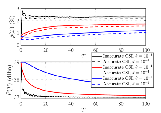
(a) All SPs adopt MRT precoding.

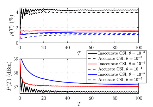
(b) All SPs adopt ZF precoding.

Figure 2: $\bar{\rho}(T)$ and $\bar{P}(T)$ vs. $T$ under different precoding schemes adopted by SPs.

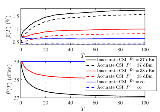
(a) All SPs adopt MRT precoding.

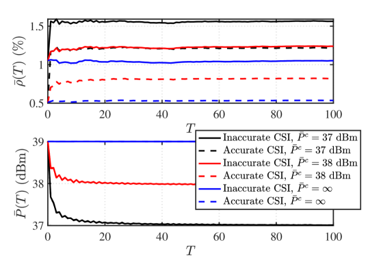
(b) All SPs adopt ZF precoding.

Figure 3: $\bar{\rho}(T)$ and $\bar{P}(T)$ vs. $T$ under different values of $\bar{P}^{c}$.

VII-1 Simulation Setup

We consider an InP that owns a virtualized network consisting of $C=7$ urban hexagon micro cells, each with radius $R=500~{}m$. The InP-owned BS at the center of cell $c\in\mathcal{C}$ is equipped with $N^{c}=32$ antennas. The InP serves $M=4$ SPs. Each SP $m$ has $K_{m}^{c}=2$ subscribing users uniformly distributed in cell $c$. Following the typical LTE specifications [31], we focus on the channel over bandwidth $B_{W}=60$ kHz, which is the sum bandwidth of $M$ subcarriers. We set the maximum transmit power limit over the channel to be $P_{\text{max}}^{c}=39~{}\text{dBm},\forall{c}\in\mathcal{C}$. Unless it is specified, we set the default average transmit power $\bar{P}^{c}=37$ dBm. The receiver noise spectral density is $N_{0}=-174$ dBm/Hz, and the noise figure is set to $N_{F}=10$ dB. At each time $t$, the channel from user $k$ of SP $m$ in cell $c$ to BS $l$ is modeled as $\mathbf{h}_{mk}^{cl}(t)=\sqrt{\beta_{mk}^{cl}}\mathbf{g}_{mk}^{cl}(t)$, where $\mathbf{g}_{mk}^{cl}(t)\sim\mathcal{CN}(\mathbf{0},\mathbf{I})$, and $\beta_{mk}^{cl}$ represents the large-scale variation. We model $\beta_{mk}^{cl}$ as [31] $\beta_{mk}^{cl}[\text{dB}]=-31.54-33\log_{10}(d_{mk}^{cl})+\psi_{mk}^{cl}$, where $d_{mk}^{cl}$ is the distance from BS $l$ to user $k$ of SP $m$ in cell $c$, and $\psi_{mk}^{cl}\sim\mathcal{CN}(0,\sigma_{\phi}^{2})$ is the shadowing with $\sigma_{\phi}=8$ dB. For a given channel $h_{mk}^{cln}$ from antenna $n$ of BS $l$ to user $k$ of SP $m$ in cell $c$, we denote $e_{\mathbf{H}}$ as the standard deviation of the normalized CSI error, i.e., $\frac{\tilde{h}_{mk}^{cln}}{|h_{mk}^{cln}|}\sim\mathcal{CN}(0,e_{\mathbf{H}}^{2})$. Finally, we assume each channel is i.i.d. over time.

To study the performance of Algorithm 2, we consider the following two metrics: First, we define the $T$-slot normalized time-averaged precoding deviation from virtualization demand as $\bar{\rho}(T)\triangleq\frac{1}{T}\sum_{t=0}^{T-1}\frac{\|\mathbf{H}^{\prime}(t)\hat{\mathbf{V}}^{\prime\star}(t)-\mathbf{D}^{\prime}(t)\|_{F}^{2}}{\|\mathbf{D}^{\prime}(t)\|_{F}^{2}}$; Second, we consider the $T$-slot time-averaged per-cell transmit power as $\bar{P}(T)\triangleq\frac{1}{TC}\sum_{t=0}^{T-1}\|\hat{\mathbf{V}}^{\prime\star}(t)\|_{F}^{2}$. We assume that the InP allocates the transmit power $P_{m}^{c}=\frac{P_{\text{max}}^{c}}{M}$ to each SP $m$, $\forall{c}\in\mathcal{C}$.

VII-2 Effect of Weight $U$

Recall that weight $U$ is a design parameter in Algorithm 2. We first study the effect of weight $U=\frac{S^{\prime}}{\epsilon}$ on the performance of the proposed algorithm by varying $\epsilon$. Note that $\bar{\rho}(T)$ is normalized to the network-wide demand $\|\mathbf{D}^{\prime}(t)\|_{F}^{2}$. We use the upper bound for $\|\mathbf{D}^{\prime}(t)\|_{F}^{2}$ in Lemma 9 to set $\epsilon$ as $\epsilon=\theta{\zeta^{\prime}}^{2}B^{2}$, where $\theta$ is used as a controllable parameter. From (1), we set $B=1.645\sqrt{\sum_{c\in\mathcal{C}}N^{c}\sum_{k\in\mathcal{K}^{c}}\beta_{k}^{c}}$, which ensures that $\mathbb{P}\{\|\mathbf{H}^{\prime}(t)\|_{F}>B\}<4.9\times 10^{-12}$ based on the Chernoff bound.

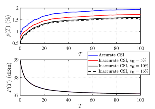
(a) All SPs adopt MRT precoding.

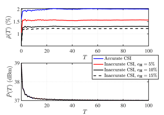
(b) All SPs adopt ZF precoding.

Figure 4: $\bar{\rho}(T)$ and $\bar{P}(T)$ vs. $T$ under different values of $e_{\mathbf{H}}$.

Figs. 2(a) and 2(b) show the time trajectory of $\bar{\rho}(T)$ and $\bar{P}(T)$ under different values of $\theta$, when all SPs adopt MRT and ZF precoding, respectively. The value of $\bar{\rho}(T)$ is shown in percentage. Both accurate and inaccurate CSI are considered. We see that the $\bar{\rho}(T)$ under inaccurate CSI closely follows that under perfect CSI. Since the power constraint does not depend on the channels, as expected, $\bar{P}(T)$ under inaccurate CSI is almost identical to that under perfect CSI. These performance in Fig. 2 demonstrate that our proposed algorithm is robust to inaccurate CSI under different precoding schemes adopted by SPs. Furthermore, we observe that our proposed algorithm converges fast (within 100 time slots) for various values of $\theta$. As $\theta$ decreases, $U$ becomes larger, which puts more emphasis on the precoding deviation $\hat{\rho}^{\prime}(t)$ than on the Lyapunov drift $\Delta(t)$ in the DPP metric. As a result, it takes a longer time for the virtual queue $\mathbf{Z}(t)$ to stabilize and for the performance to reach the steady state. In addition, for a smaller value of $\theta$, the steady state value of $\bar{\rho}(T)$ is smaller, and that of $\bar{P}(T)$ converges to $\bar{P}^{c}$. These behaviors are consistent with the bound analysis in (49) and (50) in Theorem 12. As we see, for $\theta=10^{-4}$, the average deviation $\bar{\rho}(T)$ is under $2\%$ for both the MRT and ZF precoding cases. Based on this result, we set $\theta=10^{-4}$ as the default value for the rest of simulation.

VII-3 Effect of Long-Term Transmit Power Limit $\bar{P}^{c}$

To study the effect of long-term average transmit power limit $\bar{P}^{c}$ in (39), we show in Fig. 3 the time trajectory of $\bar{\rho}(T)$ and $\bar{P}(T)$ under different values of $\bar{P}^{c}$, when all SPs adopt either MRT or ZF precoding. When $\bar{P}^{c}=\infty$, the precoding design in P3 is only subject to the short-term transmit power constraint (40). With inaccurate CSI, the steady-state value of $\bar{\rho}(T)$ is only around $0.7\%$ for MRT precoding and $1\%$ for ZF precoding. When $\bar{P}^{c}$ decreases, although $\bar{\rho}(T)$ increases for both MRT and ZF precoding schemes, their values remain small. For example, when $\bar{P}^{c}=37$ dBm, with inaccurate CSI, the steady-state value of $\bar{\rho}(T)$ is around $2\%$ for both MRT and ZF precoding schemes. As we observe, there is a trade-off between the steady-state value of $\bar{\rho}(T)$ and $\bar{P}^{c}$. The InP can use this trade-off to balance the transmit power consumption and the deviation of actual precoding from the virtualization demand.

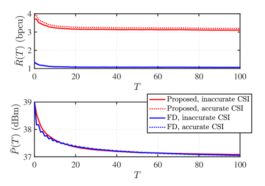
(a) MRT precoding.

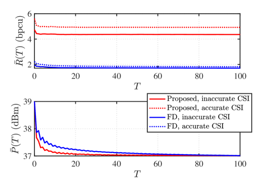
(b) ZF precoding.

Figure 5: Comparison of $\bar{R}(T)$ between the proposed approach and FD approach.

VII-4 Impact of Inaccurate CSI

In Fig. 4, we study the impact of CSI inaccuracy on the performance of the proposed algorithm by varying $e_{\mathbf{H}}$. As $e_{\mathbf{H}}$ increases from $5\%$ to $15\%$, the steady-state values of $\bar{\rho}(T)$ are still under $2\%$ for both MRT and ZF precoding schemes. Comparing the two precoding schemes, we observe that $\bar{\rho}(T)$ is more sensitive to $e_{\mathbf{H}}$ under ZF precoding than under MRT precoding. The reason is that ZF precoding requires accurate CSI to null the inter-user interference, and thus its performance is more sensitive to CSI accuracy [32]. In contrast, MRT precoding generates power gain at the general signal direction and is less sensitive to the CSI accuracy. Finally, we observe that the steady-state value of $\bar{P}(T)$ is similar for different values of $e_{\mathbf{H}}$, showing that it is not sensitive to CSI accuracy.

VII-5 Benefit of Spatial Virtualization for Service Isolation

Most existing works on MIMO WNV adopt the physical isolation approach to separate the SPs [5]-[10]. To the best of our knowledge, there is no existing online method for virtualization in multi-cell MIMO systems. Therefore, for performance comparison, we implement a physical isolation scheme for online multi-cell MIMO WNV. Specifically, we consider a frequency division (FD) scheme that allocates equal bandwidth $\frac{B_{W}}{M}$ to each SP $m$. We then use the proposed proposed online coordinated precoding solution to serve each SP. For each SP, this can be considered as a special case of Algorithm 2 with a single SP, maximum power limit $\frac{P_{c}^{\text{max}}}{M}$, and long-term power limit $\frac{\bar{P}_{c}}{M}$.

Fig. 5 shows the averaged user rate $\bar{R}(T)\triangleq\frac{1}{TK}\!\sum_{t=0}^{T-1}\!\sum_{k\in\mathcal{K}}\log_{2}\left(\!1\!+\!\frac{|[\mathbf{H}^{\prime}(t)\hat{\mathbf{V}}^{\prime}(t)]_{k,k}|^{2}}{\sum_{j\neq{k}}\!|[\mathbf{H}^{\prime}(t)\hat{\mathbf{V}}^{\prime}(t)]_{k,j}|^{2}+\sigma_{n}^{2}}\!\right)\!$ achieved by the proposed approach and the FD approach for both inaccurate CSI and accurate CSI. Note that all rates are normalized by the total bandwidth $B_{W}$. For both the MRT and ZF precoding cases, $\bar{R}(T)$ under both approaches quickly converges to its steady state. The average rate achieved by the proposed spatial isolation approach is $2{\raise 0.73193pt\hbox{$\scriptstyle\sim$}}3$ times higher that of the FD approach. This indicates substantial performance advantage of the proposed spatial isolation approach over the physical isolation approach for online virtualization in a multi-cell MIMO network.

VIII Conclusions

In this paper, we have considered designing online downlink MIMO WNV in a multi-cell network with imperfect CSI, where the InP provides a precoding solution based on the SPs’ independent service demands. Assuming fading channels and bounded CSI estimation error, we propose an online multi-cell coordinated precoding algorithm aiming to minimize the long-term time-averaged precoding deviation of the InP’s actual precoding solution from the virtualization demands by the SPs. Our proposed algorithm only depends on the imperfect CSI estimates currently available at the SPs and the InP, without the knowledge of the channel distribution. Our online coordinated precoding solution is fully distributed and in semi-closed form, which can be implemented at each cell without any CSI exchange across cells. Our analysis on the performance of the proposed online algorithm takes into account the two-fold impact of imperfect CSI on both the InP and the SPs, and we observe an optimality gap of $\mathcal{O}(\delta)$ over any time horizon due to CSI inaccuracy $\delta$. Simulation results demonstrate the effectiveness of the proposed algorithm in both convergence rate and performance robustness to imperfect CSI, as well as superior performance over the physical isolation approach.

Appendix A Proof of Lemma 7

Similar to the proof of (8) in Lemma 1. From the virtual queue updating rule in (41), the per-cell short-term power constraints (40), and $L(t)=\frac{1}{2}\sum_{c\in\mathcal{C}}Z^{c2}(t)$, we can show that

$$\Delta(t) \leq\frac{1}{2}\sum_{c\in\mathcal{C}}\max\{(P_{\text{max}}^{c}-\bar{P}^{c})^{2},\bar{P}^{c2}\}$$

$$\quad+\sum_{c\in\mathcal{C}}Z^{c}(t)(\|\hat{\mathbf{V}}^{c}(t)\|_{F}^{2}-\bar{P}^{c}).$$ (51)

Taking the conditional expectation over the virtual queue $\mathbf{Z}(t)$ and adding $U\mathbb{E}\{\hat{\rho}^{\prime}(t)|\mathbf{Z}(t)\}$ at both sides of the above inequality, we complete the proof.

Appendix B Proof of Lemma 8

Similar to the proof of (22) in Lemma 2, we can show that

$$\|\hat{\mathbf{V}}^{c\star}\|_{F}\leq\frac{U}{Z^{c}}B^{2}(1+\delta)^{2}\sqrt{N^{c}\sum_{m\in\mathcal{M}}P_{m}^{c}}.$$

It follows that the sufficient condition for $Z^{c}(t)$ to ensure $\|\hat{\mathbf{V}}^{c\star}(t)\|_{F}^{2}\leq\bar{P}^{c}$ for any time $t$ is $Z^{c}(t)\geq UB^{2}(1+\delta)^{2}\xi^{c}$. Further noting that $Z^{c}(t+1)\leq{Z}^{c}(t)+P_{\text{max}}^{c}-\bar{P}^{c}$ from (41), we complete the proof.

Appendix C Proof of Lemma 9

The proofs of the first two inequalities of (46) follow from $\|\hat{\mathbf{D}}^{\prime}(t)\|_{F}^{2}=\sum_{c\in\mathcal{C}}\|\hat{\mathbf{D}}^{c}(t)\|_{F}^{2}$ and

$$\|\hat{\mathbf{D}}^{c}(t)\|_{F}^{2} \leq\sum_{m\in\mathcal{M}}\|\hat{\mathbf{H}}_{m}^{cc}(t)\|_{F}^{2}\|\hat{\mathbf{W}}_{m}^{cc}(t)\|_{F}^{2}$$

$$\leq{B}^{2}(1+\delta)^{2}\sum_{m\in\mathcal{M}}P_{m}^{c}.$$

We now give the proof outline of the last inequality of (46). Similar to (30) and (31) in the proof of Lemma 3, we can show for any ${m}\in\tilde{\mathcal{M}}^{c}$

$$\|\mathbf{H}_{m}^{cc}(t)\mathbf{W}_{m}^{cc\text{\tiny MRT}}(t)-\hat{\mathbf{H}}_{m}^{cc}(t)\hat{\mathbf{W}}_{m}^{cc\text{\tiny MRT}}(t)\|_{F}\leq\sqrt{\alpha_{m}^{c}}B\delta$$

and for any $m\in\mathcal{M}\backslash\breve{\mathcal{M}}^{c}$

$$\|\mathbf{H}_{m}^{cc}(t)\mathbf{W}_{m}^{cc\text{\tiny ZF}}(t)-\hat{\mathbf{H}}_{m}^{cc}(t)\hat{\mathbf{W}}_{m}^{cc\text{\tiny ZF}}(t)\|_{F}\leq\sqrt{\beta_{m}^{c}}B\delta.$$

Applying the above two inequalities to

$$\|\mathbf{D}^{\prime}(t)-\hat{\mathbf{D}}^{\prime}(t)\|_{F}^{2}$$

$$=\sum_{c\in\mathcal{C}}\sum_{m\in\mathcal{M}}\|\mathbf{H}_{m}^{cc}(t)\mathbf{W}_{m}^{cc}(t)-\hat{\mathbf{H}}_{m}^{cc}(t)\hat{\mathbf{W}}_{m}^{cc}(t)\|_{F}^{2}$$

we complete the proof.

Appendix D Proof of Lemma 11

Adding $U\|\mathbf{H}^{\prime}(t)\hat{\mathbf{V}}^{\prime\star}(t)-\mathbf{D}^{\prime}(t)\|_{F}^{2}$ to both sides of (51), taking expectations, noting (47) in Lemma 10, and from the iterated law of expectation, we can show that

$$\mathbb{E}\left\{\Delta(t)\right\}+U\mathbb{E}\{\|\mathbf{H}^{\prime}(t)\hat{\mathbf{V}}^{\prime\star}(t)-\mathbf{D}^{\prime}(t)\|_{F}^{2}\}$$

$$\leq{U}\mathbb{E}\{\|\mathbf{H}^{\prime}(t)\mathbf{V}^{\prime\text{\tiny opt}}(t)-\mathbf{D}^{\prime}(t)\|_{F}^{2}\}$$

$$\quad+\mathbb{E}\left\{\mathbb{E}\left\{\sum_{c\in\mathcal{C}}Z^{c}(t)(\|\mathbf{V}^{c\text{\tiny opt}}(t)\|_{F}^{2}\!-\!\bar{P}^{c})|\mathbf{Z}(t)\right\}\right\}\!+\!U\varphi^{\prime}\!+\!S^{\prime}\!.$$

We complete the proof by noting

$$\mathbb{E}\left\{\sum_{c\in\mathcal{C}}Z^{c}(t)(\|\mathbf{V}^{c\text{\tiny opt}}(t)\|_{F}^{2}-\bar{P}^{c})|\mathbf{Z}(t)\right\}$$

$$=\sum_{c\in\mathcal{C}}Z^{c}(t)\mathbb{E}\{\|\mathbf{V}^{c\text{\tiny opt}}(t)\|_{F}^{2}-\bar{P}^{c}\}\leq 0$$

which follows from $\mathbf{V}^{c\text{\tiny opt}}(t)$ being independent of $\mathbf{Z}(t)$, $\mathbf{Z}(t)\succeq\mathbf{0}$, and $\mathbb{E}\{\|\mathbf{V}^{c\text{\tiny opt}}\|_{F}^{2}\}\leq\bar{P}^{c}$.

Appendix E Proof of Theorem 12

Rearranging term of (48), summing over time $t\in\{0,\dots,T-1\}$, dividing by $UT$, and noting that $\sum_{t=0}^{T-1}\mathbb{E}\{\Delta(t)\}=\frac{1}{2}\mathbb{E}\{\|\mathbf{Z}(T)\|_{2}^{2}\}-\mathbb{E}\{\|\mathbf{Z}(0)\|_{2}^{2}\}$, $\mathbf{Z}(0)=\mathbf{0}$, $\mathbf{Z}(t)\succeq\mathbf{0},\forall{t}$, and $U=\frac{S^{\prime}}{\epsilon}$, we have (49).

For any $c\in\mathcal{C}$, summing $\|\hat{\mathbf{V}}^{c\star}(t)\|_{F}^{2}\leq\bar{P}^{c}+Z^{c}(t+1)-Z^{c}(t)$ over $t$ yields $\frac{1}{T}\sum_{t=0}^{T-1}\|\hat{\mathbf{V}}^{c\star}(t)\|_{F}^{2}\leq\bar{P}^{c}+\frac{Z^{c}(T)}{T}$. Substituting the upper bound of the virtual queue in (45) and $U=\frac{S^{\prime}}{\epsilon}$ into the above inequality, we have (50).

References

- [1] J. Wang, M. Dong, B. Liang, and G. Boudreau, “Online precoding design for downlink MIMO wireless network virtualization with imperfect CSI,” in Proc. IEEE Conf. Comput. Commun. (INFOCOM), 2020.
- [2] C. Liang and F. R. Yu, “Wireless network virtualization: A survey, some research issues and challenges,” IEEE Commun. Surveys Tuts., vol. 17, pp. 358–380, 2015.
- [3] J. van de Belt, H. Ahmadi, and L. E. Doyle, “Defining and surveying wireless link virtualization and wireless network virtualization,” IEEE Commun. Surveys Tuts., vol. 19, pp. 1603–1627, 2017.
- [4] M. Richart, J. Baliosian, J. Serrat, and J. Gorricho, “Resource slicing in virtual wireless networks: A survey,” IEEE Trans. Netw. Service Manag., vol. 13, pp. 462–476, Sep. 2016.
- [5] V. Jumba, S. Parsaeefard, M. Derakhshani, and T. Le-Ngoc, “Resource provisioning in wireless virtualized networks via massive-MIMO,” IEEE Wireless Commun. Lett., vol. 4, pp. 237–240, Jun. 2015.
- [6] Z. Chang, Z. Han, and T. Ristaniemi, “Energy efficient optimization for wireless virtualized small cell networks with large-scale multiple antenna,” IEEE Trans. Commun., vol. 65, pp. 1696–1707, Apr. 2017.
- [7] K. Zhu and E. Hossain, “Virtualization of 5G cellular networks as a hierarchical combinatorial auction,” IEEE Trans. Mobile Comput., vol. 15, pp. 2640–2654, Oct. 2016.
- [8] S. Parsaeefard, R. Dawadi, M. Derakhshani, T. Le-Ngoc, and M. Baghani, “Dynamic resource allocation for virtualized wireless networks in massive-MIMO-aided and fronthaul-limited C-RAN,” IEEE Trans. Veh. Technol., vol. 66, pp. 9512–9520, Oct. 2017.
- [9] D. Tweed and T. Le-Ngoc, “Dynamic resource allocation for uplink MIMO NOMA VWN with imperfect SIC,” in Proc. IEEE Int. Conf. Commun. (ICC), 2018.
- [10] Y. Liu, M. Derakhshani, S. Parsaeefard, S. Lambotharan, and K. Wong, “Antenna allocation and pricing in virtualized massive MIMO networks via Stackelberg game,” IEEE Trans. Commun., vol. 66, pp. 5220–5234, Nov. 2018.
- [11] N. M. Mosharaf Kabir Chowdhury and R. Boutaba, “Network virtualization: state of the art and research challenges,” IEEE Commun. Mag., vol. 47, pp. 20–26, Jul. 2009.
- [12] M. Soltanizadeh, B. Liang, G. Boudreau, and S. H. Seyedmehdi, “Power minimization in wireless network virtualization with massive MIMO,” in Proc. IEEE Intel. Conf. Commun. (ICC) Workshops, 2018.
- [13] H. Q. Ngo, E. G. Larsson, and T. L. Marzetta, “Energy and spectral efficiency of very large multiuser MIMO systems,” IEEE Trans. Commun., vol. 61, pp. 1436–1449, Apr. 2013.
- [14] H. Dahrouj and W. Yu, “Coordinated beamforming for the multicell multi-antenna wireless system,” IEEE Trans. Wireless Commun., vol. 9, pp. 1748–1759, May 2010.
- [15] C. Shen, T. Chang, K. Wang, Z. Qiu, and C. Chi, “Distributed robust multicell coordinated beamforming with imperfect csi: An admm approach,” IEEE Trans. Signal Process., vol. 60, pp. 2988–3003, Jun. 2012.
- [16] L. Venturino, N. Prasad, and X. Wang, “Coordinated linear beamforming in downlink multi-cell wireless networks,” IEEE Trans. Wireless Commun., vol. 9, pp. 1451–1461, Apr. 2010.
- [17] Q. Shi, M. Razaviyayn, Z. Luo, and C. He, “An iteratively weighted mmse approach to distributed sum-utility maximization for a mimo interfering broadcast channel,” IEEE Trans. Signal Process., vol. 59, pp. 4331–4340, Sep. 2011.
- [18] D. W. H. Cai, T. Q. S. Quek, C. W. Tan, and S. H. Low, “Max-min SINR coordinated multipoint downlink transmission-duality and algorithms,” IEEE Trans. Signal Process., vol. 60, pp. 5384–5395, Oct. 2012.
- [19] F. Amirnavaei and M. Dong, “Online power control optimization for wireless transmission with energy harvesting and storage,” IEEE Trans. Wireless Commun., vol. 15, pp. 4888–4901, Jul. 2016.
- [20] M. Dong, W. Li, and F. Amirnavaei, “Online joint power control for two-hop wireless relay networks with energy harvesting,” IEEE Trans. Signal Process., vol. 66, pp. 463–478, Jan. 2018.
- [21] H. Yu and M. J. Neely, “Dynamic transmit covariance design in MIMO fading systems with unknown channel distributions and inaccurate channel state information,” IEEE Trans. Wireless Commun., vol. 16, pp. 3996–4008, Jun. 2017.
- [22] P. Mertikopoulos and E. V. Belmega, “Learning to be green: Robust energy efficiency maximization in dynamic MIMO-OFDM system,” IEEE J. Sel. Areas Commun., vol. 34, pp. 743–757, Apr. 2016.
- [23] P. Mertikopoulos and A. L. Moustakas, “Learning in an uncertain world: MIMO covariance matrix optimization with imperfect feedback,” IEEE Trans. Signal Process., vol. 64, pp. 5–18, Jan. 2016.
- [24] M. J. Neely, Stochastic Network Optimization with Application on Communication and Queueing Systems. Morgan & Claypool, 2010.
- [25] M. Zinkevich, “Online convex programming and generalized infinitesimal gradient ascent,” in Proc. Int. Conf. Mach. Learn. (ICML), 2003.
- [26] J. Wang, M. Dong, B. Liang, and G. Boudreau, “Online downlink MIMO wireless network virtualization in fading environments,” in Proc. IEEE Global Commun. Conf. (GLOBECOM), 2019.
- [27] J. Wang, B. Liang, M. Dong, and G. Boudreau, “Online MIMO wireless network virtualization over time-varying channels with periodic updates,” in Proc. IEEE Intel. Workshop on Signal Process. Advances in Wireless Commun. (SPAWC), 2020.
- [28] S. Boyd and L. Vandenberghe, Convex Optimization. Cambridge University Press, 2004.
- [29] A. Hjorungnes and D. Gesbert, “Complex-valued matrix differentiation: Techniques and key results,” IEEE Trans. Signal Process., vol. 55, pp. 2740–2746, Jun. 2007.
- [30] D. H. Brandwood, “A complex gradient operator and its application in adaptive array theory,” IEE Proceedings H - Microwaves, Optics and Antennas, vol. 130, pp. 11–16, Feb. 1983.
- [31] H. Holma and A. Toskala, WCDMA for UMTS - HSPA evolution and LTE. John Wiely & Sons, 2010.
- [32] R. Corvaja and A. G. Armada, “Phase noise degradation in massive MIMO downlink with zero-forcing and maximum ratio transmission precoding,” IEEE Trans. Veh. Technol., vol. 65, pp. 8052–8059, Oct. 2016.