Low-level jets and the convergence of Mars data assimilation algorithms
Abstract
\addData assimilation is an increasingly popular technique in Mars atmospheric science, but its effect on the mean states of the underlying atmosphere models has not been thoroughly examined. The robustness of results to the choice of model and assimilation algorithm also warrants further study. We investigate \changethe effect of data assimilation on the mean climates ofthese issues using two Mars general circulation models (MGCMs), with particular emphasis on zonal wind and temperature fields. When temperature retrievals from the Mars Global Surveyor Thermal Emission Spectrometer \add(TES) are assimilated into the U.K.-Laboratoire de Météorologie Dynamique (UK-LMD) MGCM to create the Mars Analysis Correction Data Assimilation (MACDA) reanalysis, low-level zonal jets in the winter northern hemisphere shift equatorward and weaken relative to a free-running control simulation from the same MGCM. The Ensemble Mars Atmosphere Reanalysis System (EMARS) reanalysis, which \changeassimilates essentially the sameis also based on TES temperature retrievals, also shows jet weakening (but \changenotless if any shifting) relative to a control simulation performed with the underlying Geophysical Fluid Dynamics Laboratory (GFDL) MGCM. \removeFor both reanalysis–control simulation pairs, the low-level extratropical jet changes caused by data assimilation are associated with surface pressure changes. These surface pressure changes are roughly in geostrophic balance with the wind changes. Examining higher levels of the atmosphere, monthly mean three-dimensional temperature and zonal wind fields are in \changerobustlygenerally better agreement between the two reanalyses than between the two control simulations. \removeFurthermore, the MACDA control run typically differs more from MACDA than the EMARS control run differs from EMARS. In conjunction with information about the MGCMs’ physical parametrizations, intercomparisons between the various reanalyses and control simulations suggest that \addoverall the EMARS control run is \changegenerallyplausibly less biased (relative to the true state of the Martian atmosphere) than the MACDA control run. Implications for future observational studies are discussed.
Department of the Geophysical Sciences, University of Chicago, Chicago, Illinois, USA Department of Physics, University of Maryland, Baltimore County, Baltimore, Maryland, USA Department of Meteorology and Atmospheric Science, The Pennsylvania State University, University Park, Pennsylvania, USA Now at Department of Earth and Planetary Sciences, Harvard University, Cambridge, Massachusetts, USA
Todd A. Mooringtmooring@alum.mit.edu
Assimilating temperature data \changeintoin UK-LMD Mars \changeatmosphereclimate model weakens\change and, shifts northern \addwinter low-level jet, but has less effect on GFDL model
Time mean flows generally agree better in the MACDA and EMARS reanalyses than in their associated \changefree-running control simulationscontrol runs
Reanalysis–control run mean state differences suggest that the EMARS control run has smaller biases than the MACDA control run
Plain Language Summary
An increasingly popular way to study Martian weather and climate is to combine atmospheric temperature observations with a computer model (specifically, a general circulation model). The process of combining model and observations is referred to as “data assimilation”, and the resulting merged data set is referred to as a “reanalysis”. Several Mars reanalyses have been produced. One advantage of reanalyses is that they include meteorological variables (such as wind) that are not directly observed—however, it is not clear how accurately data assimilation algorithms compute these unobserved variables. Our study investigates this issue using two Mars reanalyses and two model simulations that do not assimilate temperature data. We focus on slowly-varying atmospheric phenomena (timescales from 10 Mars days to a season). Assimilating temperature data into two different general circulation models changes the strength and/or spatial pattern of east-west winds at low altitudes. Furthermore, monthly mean three-dimensional temperature and east-west wind fields agree better between reanalyses than between non-assimilating model simulations. This suggests that the data assimilation process is basically successful. One non-assimilating model simulation has less realistic representations of atmospheric physical processes than the other—we argue that this \changelikelyplausibly gives it larger biases relative to the true state of the atmosphere.
1 Introduction
Data assimilation for the Martian atmosphere has been a subject of research for more than two decades [Lewis \BBA Read (\APACyear1995), Lewis \BOthers. (\APACyear1996), Houben (\APACyear1999)] and recent years have seen a proliferation of reanalysis data sets [<]e.g.,¿[]montabone14,steele14,navarro17,holmes18,greybush19gdj,holmes19,holmes20. The Martian data assimilation problem must be solved with fewer and different observations than its terrestrial counterpart: to date, \changethe only data directly used to update the atmospheric dynamical state during the assimilation process are infrared temperature retrievals or their underlying radiancesMars reanalysis efforts have been highly dependent on infrared temperature retrievals (or at least their underlying radiances) in ways that Earth reanalyses are not [<]e.g.,¿[]lee11,montabone14,greybush19gdj, [<]cf.¿[]gelaro17,hersbach20. \changeOtherThis is because other dynamical information, such as surface pressure or wind observations, is available with only very limited spatial coverage [Hinson (\APACyear2008), Martínez \BOthers. (\APACyear2017)].
From a dynamical perspective, atmospheric temperature structure is most clearly informative about wind fields via thermal wind or similar balance arguments [<]e.g.,¿[]banfield04. However, thermal wind is at best a theory of the vertical wind shear—it cannot constrain the absolute wind at the surface and is also expected to break down in the tropics. Thus although the large-scale near-surface and tropical atmospheric circulations are basic features of the Martian climate system, it is not obvious how well they are estimated by data assimilation systems [Lewis \BOthers. (\APACyear1996), Lewis \BOthers. (\APACyear1997), Hoffman \BOthers. (\APACyear2010)]. Nor are the simulations of these features by free-running Mars general circulation models (MGCMs) easy to validate.
Here we \changeinvestigatebegin to address these product quality issues by investigating how assimilating temperature retrievals into MGCMs changes their climatological mean states, with particular emphasis on zonal winds. To explore the robustness of our results, we examine two different reanalyses and their associated control simulations—the control simulations differ from the reanalyses primarily by not assimilating temperature retrievals. The use of two reanalysis–control run pairs also allows us to expand on previous investigations [Waugh \BOthers. (\APACyear2016), Greybush, Gillespie\BCBL \BBA Wilson (\APACyear2019)] of whether different data assimilation systems are able to converge on a single atmospheric state. Ultimately we are able to draw some \addtentative conclusions about the \removelikely quality of the reanalyses and control simulations, even without using any independent validation data.
TThe main body of this paper is divided into four major sections. We summarize the reanalysis data sets and control simulations in section 2. Results on the low-level zonal mean jets are presented in section 3, while the vertical and meridional structure of the zonal mean temperature and zonal wind fields is examined in section 4. The extent to which data assimilation converges the time mean states of the two MGCMs is addressed more formally in section 5. A summary and discussion of implications for future observational work concludes the paper\add, and three appendices present results of sensitivity tests and additional statistical details.
2 Reanalysis and control simulation data sets
We use the Mars Analysis Correction Data Assimilation version 1.0 [<]MACDA,¿[]montabone14 and Ensemble Mars Atmosphere Reanalysis System version 1.0 [<]EMARS,¿[]greybush19gdj reanalyses, both of which assimilate \changeessentially the same temperature data—retrievalstemperature retrievals from the Mars Global Surveyor Thermal Emission Spectrometer [<]TES,¿[]conrath00. This gives the two reanalyses similar temporal extents: MY24 141∘ (103∘) to MY27 86∘ (102∘) for MACDA (EMARS), where the Mars years (MY) and seasonal dates are defined using the \citeAclancy00 calendar. However, occasional gaps in the availability of TES retrievals mean that the reanalyses are not constrained by observations throughout the full lengths of these periods. Ten intervals in which the reanalyses are thought to be poorly constrained are excluded from our study, generally following Table S1 of \citeAmooring15. (Two more such intervals occur near the beginning of the EMARS data set, but are rendered irrelevant by our choice to ignore the period prior to MY24 135∘. \addWe also do not use the MY28-33 segment of EMARS based on Mars Climate Sounder retrievals.)
The two reanalyses are underpinned by substantially different MGCMs and data assimilation algorithms. MACDA is based on the U.K.-Laboratoire de Météorologie Dynamique (UK-LMD) MGCM with a spectral dynamical core [Forget \BOthers. (\APACyear1999)]. The MACDA version of this model was integrated with a horizontal resolution of T31 and 25 sigma levels [Montabone \BOthers. (\APACyear2006)], and the MACDA output data are available on a 5∘ latitude-longitude grid. EMARS uses a version of the Geophysical Fluid Dynamics Laboratory (GFDL) MGCM with a finite-volume dynamical core on a latitude-longitude grid [<]e.g.,¿[]hoffman10. The horizontal resolution of this model is 5∘ latitude 6∘ longitude, and it has 28 hybrid sigma-pressure levels.
MACDA assimilates temperature retrievals using the analysis correction method [Lewis \BOthers. (\APACyear2007)], which updates the model state every dynamical timestep (480 times per sol—a sol is a Martian mean solar day, 1.03 Earth days). In contrast, EMARS assimilates temperature retrievals 24 times per sol using an ensemble Kalman filter [Hoffman \BOthers. (\APACyear2010), Zhao \BOthers. (\APACyear2015)]. The MACDA data set is available 12 times per sol [Montabone \BOthers. (\APACyear2014)], while EMARS analyses are available 24 times per sol [Greybush, Kalnay\BCBL \BOthers. (\APACyear2019)]. \changeThe (Mars) hourly background forecasts, which the ensemble Kalman filter updates to form the analyses, are also available 24 times per sol. Because the EMARS background forecasts share the same horizontal grid as the output files from the EMARS control simulation, while the EMARS analyses do not, we opted to use the background forecasts (rather than the analyses per se) as EMARS’s observationally-constrained representation of the Martian atmospheric state.Note that the publicly available EMARS output consists of both analyses and short (1 Mars hour) background forecasts—although many atmospheric variables are available as forecasts only, the pressure, temperature, and wind variables needed for this study are available as both analyses and forecasts and we opt to use the former as they are (slightly) more observationally constrained.
The free-running control simulations are essentially identical to their associated reanalyses, \changewith two major exceptionsexcept that by definition they do not assimilate temperature retrievals. \changeFirst, by definition the control simulations do not assimilate temperature retrievals. Second, although the MACDA control simulation covers the same multi-Mars year period as MACDA, the EMARS control simulation has a length of only 1.2 Mars years (MY24 103∘ to MY25 180∘)—in contrast to the 3 Mars years of EMARS itself.It is important to emphasize that the EMARS control simulation used in this study (version 1.02) is substantially longer than the (version 1.0) control simulation described in \citeAgreybush19gdj, \addwhich covered only 1 Mars year of the TES era. The MACDA and EMARS control simulations will hereinafter be referred to as MCTRL and ECTRL, respectively.
Even though the control simulations are not constrained by temperature retrievals, they can still be identified with specific Mars years and seasons because their dust fields are time-dependent and constrained by observations. For MACDA and MCTRL, TES-based column opacities are assimilated using the analysis correction method [Montabone \BOthers. (\APACyear2014)]—however, this particular version of the UK-LMD MGCM does not transport dust so the “forecast model” underlying the dust opacity assimilation is simply persistence. Given the analyzed column opacities, MACDA and MCTRL distribute the opacity in the vertical using a Conrath-like distribution [Conrath (\APACyear1975), Montabone \BOthers. (\APACyear2006)]. In contrast, the three-dimensional dust fields in EMARS and ECTRL evolve under the influences of wind advection and sedimentation [Greybush, Kalnay\BCBL \BOthers. (\APACyear2019)]. Agreement with observational data is maintained by nudging the column opacities towards the time-dependent dust maps of \citeAmontabone15\add, which can also be considered a simple form of data assimilation. Note that the \citeAmontabone15 dust maps for the period in question are based on retrievals not only from TES, but also from the Thermal Emission Imaging System (THEMIS) on Mars Odyssey.
3 Low-level zonal jets
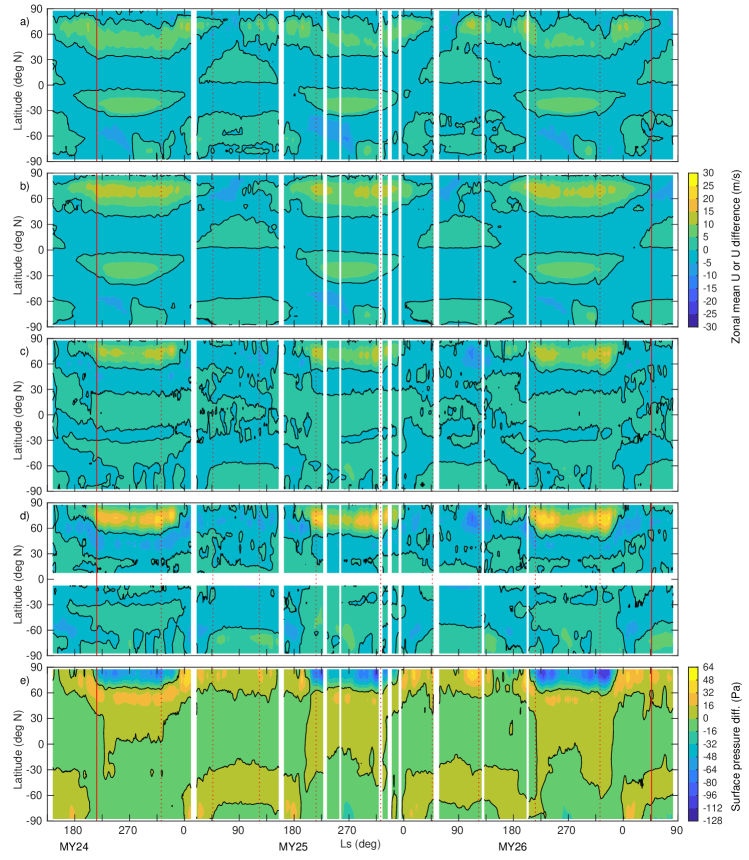
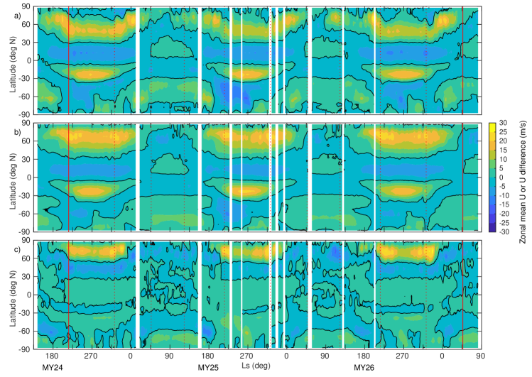
We begin our comparison of the reanalysis and control run circulations by examining seasonally-resolved zonal mean zonal winds on the (90 m above ground) level in MACDA and MCTRL. Northern (southern) winter solstice occurs at 270∘ (90∘), and focusing initially on the northern hemisphere during its local winter we see that the peak strength of the extratropical zonal jet is lower in MACDA (Figure 1a) than in MCTRL (Figure 1b). The control run jet also tends to be farther poleward than its reanalysis counterpart. This point is clarified in Figure 1c, which shows the difference between the MCTRL and MACDA fields. Figure 1c also reveals qualitatively similar behavior in the southern hemisphere near local winter solstice, which was masked in the previously mentioned figure panels by the usually weaker southern winter extratropical near-surface jet. Generally similar wind results are found on the (1.1 km above ground) level (A, Figure 5). Furthermore, the MACDA–MCTRL jet differences are associated with differences in zonal mean surface pressure (Figure 1e). The differences in surface pressure shown in Figure 1e are qualitatively consistent with geostrophic balance and the wind differences shown in Figure 1c, although the surface geostrophic zonal wind differences are \addoften stronger than the actual wind differences at (Figure 1d).
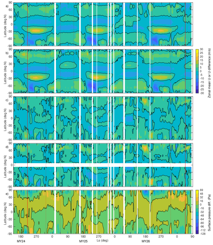
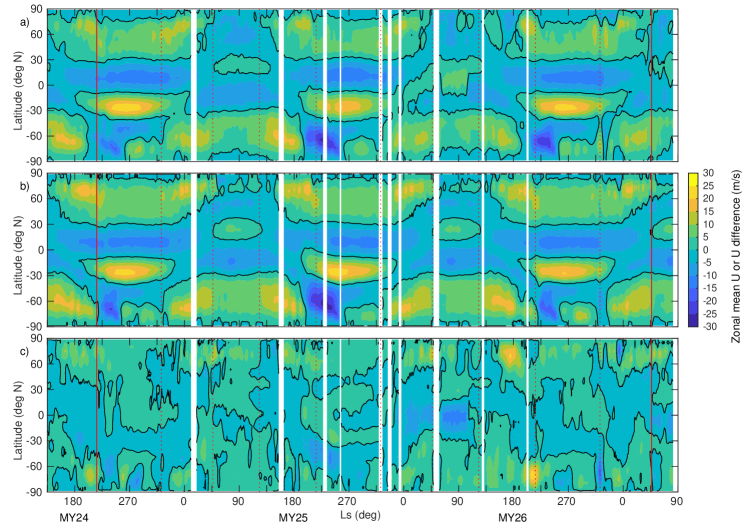
A comparable analysis of EMARS and ECTRL yields notably different results (Figure 2). \changeAlthough the relatively short length of ECTRL limits the temporal extent of a direct comparison between the two data sets, thereThere is a tendency for the assimilation of temperature data to weaken the extratropical winter jets \addnear 60∘ latitude in both hemispheres (Figure 2a-\changebc). However, in contrast to the situation with the UK-LMD MGCM, \removedata assimilation has no obvious effect on the position of the zonal jets—the EMARS–ECTRL jet difference field (Figure 2c) lacks the clear extratropical dipolar structures seen in its MACDA–MCTRL counterpart (Figure 1c).\adddata assimilation has no obvious effect on the position of the zonal jets—the clear extratropical dipolar structures seen in the MACDA–MCTRL jet difference field (Figure 1c) \addare absent or greatly weakened in its EMARS–ECTRL counterpart (Figure 2c). The maximum magnitudes of control–reanalysis \addnorthern winter jet differences appear to be smaller for EMARS–ECTRL than for MACDA–MCTRL\remove, at least in the northern hemisphere (Figures 1c and 2c). As with the UK-LMD MGCM, comparable results are found when winds are evaluated on a model level with (1.0 km above ground, Figure 6). \changeNote also thatInterestingly, the data assimilation effect on surface pressure gradients has a different seasonality in the GFDL MGCM than in the UK-LMD MGCM—for example, the structure of the EMARS–ECTRL northern hemisphere pressure difference field (Figure 2e) changes substantially during the \addMY24 and MY25 225∘–315∘ seasonal interval\adds but the corresponding MACDA–MCTRL field does not (Figure 1e). \addFurthermore, even the typical sign of the data assimilation effect on northern hemisphere summer pressure gradients differs between the GFDL and UK-LMD MGCMs (Figure 1e and 2e). However, as for MACDA–MCTRL the EMARS–ECTRL surface geostrophic wind differences (Figure 2d) effectively capture the actual patterns of low-level zonal wind differences.
Finally, we note in passing a dubious and previously undocumented feature of EMARS. Starting near MY26 0∘ and continuing to 105∘, the zonal near-surface winds are typically westerly at the equator (Figures 2a and 6a\add). This is in stark contrast to the winds at this season in MY25 and MY27 of EMARS, and in all Mars years of ECTRL (Figures 2b and 6b\add). The abrupt transition to easterly winds near MY26 105∘ is coincident with the switch from the second to the third of the separately-initialized EMARS production streams [Greybush, Kalnay\BCBL \BOthers. (\APACyear2019)]\add, and is therefore almost certainly an artifact. Although the pre-transition westerlies are clearly an outlier relative to the rest of EMARS and all of ECTRL, a more definitive assessment of whether the pre-transition westerlies or post-transition easterlies are more realistic requires additional research.
4 Latitude-pressure structure of zonal mean fields
Unfortunately, there are very few observations directly sensitive to wind in the lower atmosphere of Mars—anemometers on a handful of landers [<]e.g.,¿[]martinez17, geostrophic winds from radio occultations [<]e.g.,¿[]hinson99, and arguably cloud-tracked winds from orbiter imagery [Wang \BBA Ingersoll (\APACyear2003)]. The potential for a direct validation of reanalysis-based winds is thus limited. However, we can much more readily evaluate the extent to which MACDA and EMARS converge to the same solution—as they should, to the extent that the assimilated data can effectively constrain and correct biases in the MGCM states. Although our ultimate goal in this paper is to conduct a novel intercomparison of the three-dimensional time mean states of MACDA, EMARS, and their control simulations, we will lead into such an analysis with an examination of zonally-averaged time mean fields.
Because of the strong seasonality of the Martian atmosphere and the limited temporal extent of ECTRL, we will analyze 668 sols of data (almost exactly 1 Mars year) beginning at MY24 144∘. This period is divided into four 167-sol seasons essentially centered on solstices and equinoxes: boreal winter, spring, summer, and autumn are thus 216∘–322∘, 322∘–46∘, 46∘–123∘, and 123∘–216∘, respectively. The 668 sols beginning at MY24 144∘ are marked in Figures 1 and 2 with solid red lines, while borders between the seasons are marked with dashed red lines. (The boreal autumn mean combines data from both MY24 and MY25.)
Because of the strong seasonality of the Martian atmosphere, for this analysis we will divide the Martian annual cycle into four seasons of nearly equal length and essentially centered on the solstices and equinoxes. More specifically, we define boreal winter, spring, summer, and autumn as 216∘–322∘, 322∘–46.7∘, 46.7∘–123∘, and 123∘–216∘. The 2.5 Mars year interval from MY24 216∘ to MY27 46.7∘ then consists of exactly 10 seasons—three (two) realizations each of boreal winter and spring (summer and autumn). In Figures 1 and 2\add, the beginning and end of this 2.5 Mars year period are marked with solid red lines and the borders between individual seasons are marked with dashed red lines.
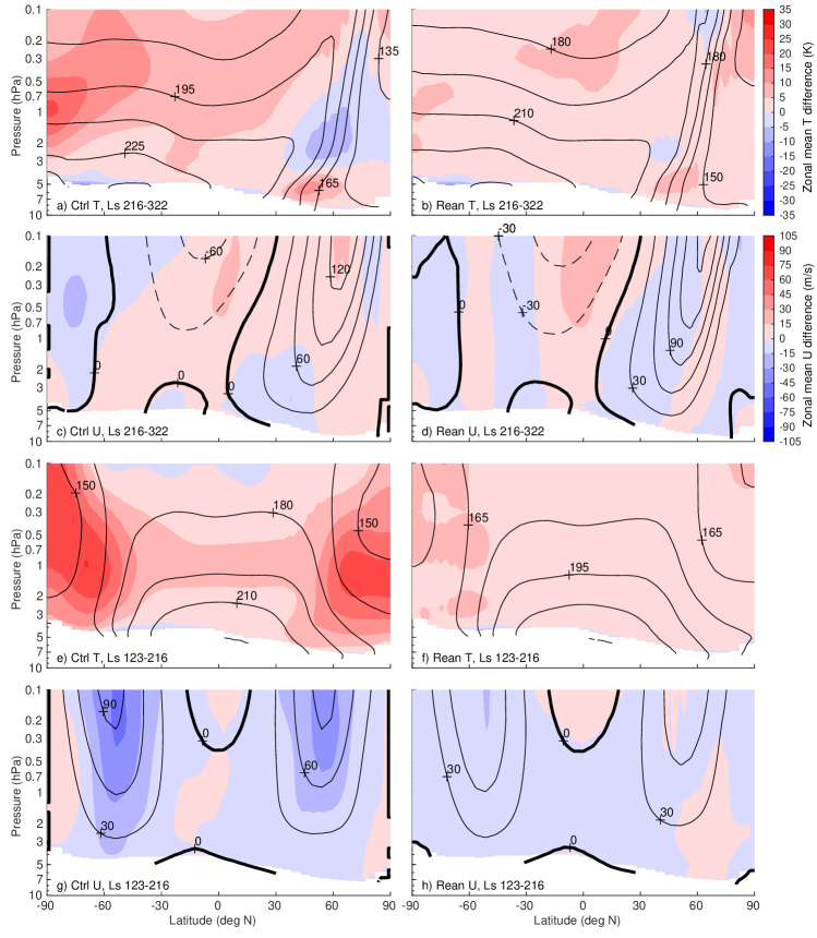
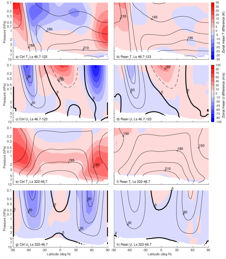
An initial examination of the vertical and meridional structures of zonal mean temperature and zonal wind fields suggests that assimilating TES temperature retrievals brings the UK-LMD and GFDL MGCM states closer together. Results for 123∘–216∘ and 216∘–322∘ are shown in Figure 3. Although ECTRL is able to basically reproduce the seasonal variations seen in EMARS (black contours), the disagreements (red and blue shading) between MCTRL and ECTRL (Figure 3a, c, e, g) tend to be larger than those between MACDA and EMARS \addexcept possibly for the 216∘–322∘ zonal winds (Figure 3b, d, f, h). While MACDA is often warmer than EMARS (Figure 3b, f), maximum temperature disagreements for these seasons are larger in the free-running control simulations than in the reanalyses: for example, MCTRL can be more than 20 K warmer than ECTRL in the polar regions (Figure 3a, e). \changeDue to thermal wind balance, these temperature disagreements imply larger jet disagreements between the control simulations than between the reanalysesThese patterns of temperature disagreement are associated with jet disagreement due to thermal wind balance—such disagreements are often but not always larger in the control simulations, especially in the extratropics for 123∘–216∘ and in high southern latitudes for 216∘–322∘ (Figure 3c, d, g, h). A tendency of temperature assimilation to converge the UK-LMD and GFDL MGCM mean states is also seen for the other two seasons (Figure 4). \changeWhileAlthough the patterns of difference between MCTRL and ECTRL are much alike in the two equinox seasons (Figures 3e, g and 4e, g), they appear to disagree more strongly during boreal summer than during boreal winter (Figures 3a, c and 4a, c).
5 Convergence of three-dimensional mean fields
We can obtain more systematic and quantitative results by computing root mean square (RMS) differences between the various free-running MGCM and reanalysis data sets. For some three-dimensional time mean field , let us denote the \add(area- and mass-weighted, assuming hydrostatic balance) RMS difference between data sets and as . \changeWeMore precisely, we define by
| (1) |
where and are field from data sets and , and are the pressures of the top and bottom of the region of interest, and denotes the latitude range(s) of interest—the domain over which the meridional integral is taken need not be continuous.
It is worth explaining our definition of the time mean. \addOur interest is in the mean state of the atmosphere, so the averaging period must be chosen long enough to average out the transient eddies. However, an excessively long averaging period would needlessly erase information about any shorter-term changes in the mean state. \changeFor these RMS difference calculations, we opt to split the 1 Mars year period we are analyzing into 16 months, by subdividing each of the four seasons into four months of 41.75 sols apiece.We will again analyze the 2.5 Mars year interval from MY24 216∘ to MY27 46.7∘ and will attempt to balance these two competing goals by dividing each of the 10 seasons defined in section 4\add into four months with approximately equal lengths of 41.8 sols. We then take time means over each of the 40 such months—although because we exclude periods not well constrained by TES data (section 2, Figures 1 and 2\add), four of these monthly means are based on less than 30 sols of data apiece. Time averaging over \changeperiods this long41.8-sol months should suffice to suppress most transient eddy variability [<]e.g.,¿[]banfield04,mooring15—to the extent that this goal is achieved, any improvement in the agreement of monthly means due to assimilation of TES temperature retrievals should come from correcting the MGCMs’ time mean biases and not from synchronizing their unforced variability. Indeed, repeating the analyses \changeusing 12 months of 55 solswith a month redefined as one-third of a season (55.7 sols) did not qualitatively change the main results (B).
We evaluate equation 1 for each of the \change1640 months for two choices of , 10 (overlapping) spatial regions of interest, and all six possible unique pairs of data sets. The fields used are temperature and zonal wind, and is either 0.1 or 3 hPa. is a spatially-varying monthly mean surface pressure. Specifically, for each location it is computed as the minimum of the four individual data set (MACDA, MCTRL, EMARS, ECTRL) monthly means after the data sets have all been interpolated to a single grid. The choice of = 0.1 hPa excludes altitudes above those directly influenced by TES temperature profile assimilation [Lewis \BOthers. (\APACyear2007)], while using = 3 hPa emphasizes the lower part of the atmosphere for greater comparability to the results in section 3.
The 10 spatial regions are formed by combining the two pressure ranges with five latitude ranges: global (90∘S–90∘N), tropics (30∘S–30∘N), northern and southern hemisphere extratropics (30∘–90∘N and 30∘–90∘S, respectively) and all extratropics (the union of northern and southern extratropics). While the various latitude ranges are clearly not all independent, using multiple latitude bands is helpful for checking the robustness of the results and investigating whether the effectiveness of temperature assimilation in converging different MGCM mean states varies meridionally.
By comparing the relative sizes of the different we provide support for two major claims:
-
1.
Assimilating temperature retrievals into the MGCMs brings their monthly mean states into better agreement
-
2.
ECTRL is \changeprobablyplausibly less biased (with respect to the true monthly mean states of the Martian atmosphere) than MCTRL
Knowledge of the actual values of the is not necessary to support these claims—instead, the results are presented in Table 1 in terms of the numbers of months (out of \change1640 possible) for which various inequalities involving the six are satisfied. \addFor compactness of notation, in these inequalities we will denote MACDA, MCTRL, EMARS, and ECTRL as , , , and , respectively.
We support the first claim by examining the inequality
| (2) |
Physically, this inequality will be satisfied if the free-running control simulations are in better agreement than the reanalyses are (for the given month, field, and region of interest). If this is the case, it means that assimilating TES temperature retrievals does not systematically bring the monthly mean states of the UK-LMD and GFDL MGCMs together—contrary to the impression created by Figures 3 and 4.
| Field | Domain | Meridional | ||||
|---|---|---|---|---|---|---|
| top (hPa) | domain | |||||
| T | 0.1 | Global | 7 | 14 | ||
| T | 0.1 | Tropics | 1 | 5 | 6 | |
| T | 0.1 | SH extratropics | 12 | 2 | 11 | |
| T | 0.1 | NH extratropics | 12 | 7 | 24 | |
| T | 0.1 | All extratropics | 8 | 3 | 18 | |
| T | 3 | Global | 11 | 2 | 7 | |
| T | 3 | Tropics | 3 | 4 | 3 | |
| T | 3 | SH extratropics | 5 | 12 | 3 | 8 |
| T | 3 | NH extratropics | 15 | 6 | 15 | |
| T | 3 | All extratropics | 12 | 3 | 7 | |
| U | 0.1 | Global | 1 | 10 | 19 | |
| U | 0.1 | Tropics | 17 | 18 | ||
| U | 0.1 | SH extratropics | 8 | 6 | 1 | 14 |
| U | 0.1 | NH extratropics | 1 | 9 | 6 | 28 |
| U | 0.1 | All extratropics | 4 | 28 | ||
| U | 3 | Global | 4 | 16 | 2 | 13 |
| U | 3 | Tropics | 18 | 26 | 5 | |
| U | 3 | SH extratropics | 13 | 11 | 3 | 4 |
| U | 3 | NH extratropics | 8 | 11 | 6 | 20 |
| U | 3 | All extratropics | 2 | 11 | 1 | 15 |
| This table contains information about relative levels of agreement between the various reanalysis and | ||||||
| control simulation data sets. We denote the RMS difference between data sets and as . | ||||||
| The left three columns name the variable being analyzed and the region over which RMS differences | ||||||
| are being computed. The right four columns contain the results, expressed as the number of months (of \change1640 | ||||||
| total) for which the inequality given at the top of each column is satisfied. Zeros have been | ||||||
| omitted for clarity. As an example of how to read the table, the large number of \change(implied) zerosvalues 40 in | ||||||
| the column means that EMARS is in robustly better agreement | ||||||
| with ECTRL than with MCTRL. | ||||||
In practice, equation 2 is generally not satisfied—Table 1 indicates that equation 2 is true in at most \change618 and often many fewer of the \change1640 total months. If consideration is restricted to the global or all-extratropics meridional regions, the inequality is satisfied for at most \changeonefour month\adds. These results strongly suggest that assimilation of the same temperature retrievals into UK-LMD and GFDL MGCM simulations tends to bring together not merely their instantaneous weather conditions, but also their climates as measured by monthly means—a more formal statistical analysis suggests that if data assimilation had no effect whatsoever on the MGCMs’ monthly mean states, it is unlikely that these results would have been obtained (C). \addPerhaps unsurprisingly, the tendency for data assimilation to converge the monthly means appears stronger for temperature than for zonal wind—for a given region, equation 2\add is always satisfied in at least as many months for zonal wind as for temperature.
We begin to support the second claim by examining
| (3) |
If satisfied, this inequality indicates that the UK-LMD reanalysis–control run pair is in better agreement than the GFDL reanalysis–control run pair. \changeHowever, aAcross all of the different field–region combinations equation 3 is satisfied in \changeno more than 8as many as 26 months (Table 1). \changeExcluding the = 3 hPaHowever if the tropical zonal wind\removes case\adds are excluded, it is never satisfied in more than \change516 months. \changeEvidentlyThis is evidence (albeit not always very strong) that EMARS and ECTRL are generally in better agreement than MACDA and MCTRL\add, at least outside the tropics. One possible explanation for this \changefindingapparent result is that ECTRL is less biased (relative to the truth) than MCTRL. However, we cannot immediately dismiss the possibility that the ECTRL biases are comparable to or larger than those of MCTRL but that the EMARS ensemble Kalman filter is simply less effective than the MACDA analysis correction scheme at adjusting the mean state of a biased MGCM.
We can separate these possibilities using the additional inequalities
| (4) |
and
| (5) |
The former (latter) characterizes how well the two control simulations verify against EMARS (MACDA). If ECTRL were clearly superior to MCTRL (in the sense of verifying better against both reanalyses) then equation 5 would often be satisfied and equation 4 would not be. Likewise, if MCTRL were superior equation 4 would often be satisfied and equation 5 would not be. Alternatively, if both reanalyses were strongly biased toward their underlying MGCMs both equation 4 and equation 5 would be only rarely satisfied.
The results support the idea that ECTRL is generally less biased than MCTRL—equation 4 is satisfied in \change37 months at most but equation 5 is satisfied in as many as \change1328 months (Table 1). Furthermore, for \changea given field and regionmost field–region combinations equation 5 is \removealways satisfied \changefor at least as manyin more months \changeasthan equation 4\add—the exceptions are the tropical zonal wind cases. Statistical analysis suggests that these results\change —at least for the spatial regions that have = 0.1 hPa and are not wholly tropical—are unlikely to be explicable as pure interval variability\change—in other words,. In practice, this implies that ECTRL and MCTRL have distinct climates and are not simply different realizations of internal variability from a single climate (C). Note also that for \changesomecertain field–region combinations both equation 4 and equation 5 are rarely or never satisfied\change—this is, consistent with the idea that the reanalyses have some tendency to inherit the climates of their underlying MGCMs. \addThis phenomenon is particularly prominent in the tropics.
Indeed, there are physical reasons to expect ECTRL to be less biased than MCTRL. Although both control simulations have their column dust opacities constrained to follow similar observational data sets, the constraint method used for ECTRL is more \changefullyclearly consistent with the physics of dust transport in the atmosphere as described in section 2. Previous work suggests that this should yield more realistic temperatures [Wilson \BOthers. (\APACyear2008)]. Also, the Martian atmosphere features water ice clouds which are thought to substantially affect the thermal structure and circulation [<]e.g.,¿[]wilson08,mulholland15. Parameterizations of the radiative effects of water ice clouds have been developed for both the GFDL and UK-LMD MGCMs [<]e.g.,¿[]hinson04,mulholland15. They are used in the EMARS–ECTRL version of the GFDL model, but not in the MACDA–MCTRL version of the UK-LMD model [Forget \BOthers. (\APACyear1999), Montabone \BOthers. (\APACyear2014), Greybush, Kalnay\BCBL \BOthers. (\APACyear2019)]. Since the physical parameterizations of ECTRL are a priori more realistic than those of MCTRL, it would be unsurprising if the output of the former simulation were closer to the truth.
6 Summary and discussion
We have presented a systematic intercomparison of slowly-varying components of the circulation in two Mars reanalyses and their associated free-running control simulations. The reanalyses assimilate essentially the same temperature retrievals, but via very different algorithms and into two distinct Mars general circulation models. Nevertheless, the three-dimensional monthly mean temperature and zonal wind fields are generally in better agreement for the reanalyses than for the control simulations. This suggests a certain robustness of Mars reanalyses to the choice of MGCM and assimilation algorithm, in agreement with \citeAwaugh16 and \citeAgreybush19te.
We devote particular attention to the low-level extratropical zonal mean zonal jets. Assimilating temperature retrievals into the UK-LMD MGCM to create MACDA tends to weaken the northern hemisphere winter jet and to shift it equatorward. Roughly similar shift behavior is found for southern hemisphere winter as well. Weakening of low-level winter jets also results when temperatures are assimilated into the GFDL MGCM, although the overall effect is more subtle than for the UK-LMD MGCM. Furthermore, changes in surface pressure gradients occur in response to temperature assimilation—these are qualitatively consistent with geostrophic balance, most evidently for northern hemisphere winter in the UK-LMD MGCM.
Finally, we have produced evidence that (at least in \changea globalan average sense) the EMARS control simulation is less biased than the MACDA control simulation. Note that this result is not guaranteed to hold for individual meridional or vertical regions, such as the tropics or pressures 3 hPa—indeed, our results are consistent with the idea that the reanalyses inherit biases from their underlying MGCMs for at least some regions and fields.
Our results suggest that the low-level zonal jets of MGCMs may be biased and that similar biases might be shared across multiple MGCMs. Studies of low-level circulations in the Martian atmosphere would thus benefit from collection of additional data more sensitive to near-surface wind or pressure fields. Technological options for collecting such data include lander networks [<]e.g.,¿[]harri17, radio occultation constellations [<]e.g.,¿[]kursinski12, and orbiting wind lidars [<]e.g.,¿[]cremons20. Alternatively, it may be possible to derive improved constraints on low-level zonal geostrophic winds from existing radio occultation and/or lander data. Further MGCM experiments and reanalysis diagnostic studies are also needed to understand the origins of the MGCM–reanalysis and inter-reanalysis disagreements documented here.
Appendix A Sensitivity of low-level jets to altitude
Our primary examination in section 3 of the seasonal and meridional variations of low-level zonal jets evaluated them on model levels roughly 0.1 km above ground (Figures 1 and 2). To make sure our findings are not strongly sensitive to this arbitrary altitude choice, we repeated the analysis on model levels roughly 1 km above ground and show the results in Figures 5 and 6. Jet behavior at the two altitudes is basically similar.
Appendix B RMS difference calculation with \change1230 \change5555.7-sol months
To verify that our results concerning the three-dimensional time mean states are robust to the somewhat arbitrary choice of averaging period, we repeated the root mean square (RMS) difference calculations \changeusing 12 months of 55 sols apiece instead of the standard 16 41.75-sol monthswith each of the 10 seasons divided into three months of 55.7 sols apiece. \removeNote that these new longer months evenly divide the 668-sol analysis period and thus do not evenly divide the four seasons defined in the main paper—in other words, some of the new months overlap the season boundaries.Tables 2 and 3 are the \change5555.7-sol month counterparts of Tables 1 and 4, respectively. \addWhile the exact quantitative results differ from those obtained with the 41.8-sol months, the qualitative summary text in section 5\add is based on all four tables and as such is robust to the choice of a 41.8-sol or 55.7-sol averaging period.\removeWe see that the most important results obtained with 41.75-sol months are reproduced here: [table struck]
| Field | Domain | Meridional | ||||
|---|---|---|---|---|---|---|
| top (hPa) | domain | |||||
| T | 0.1 | Global | 5 | 12 | ||
| T | 0.1 | Tropics | 1 | 3 | 5 | |
| T | 0.1 | SH extratropics | 7 | 1 | 8 | |
| T | 0.1 | NH extratropics | 11 | 5 | 17 | |
| T | 0.1 | All extratropics | 8 | 3 | 14 | |
| T | 3 | Global | 7 | 6 | ||
| T | 3 | Tropics | 2 | 1 | 2 | |
| T | 3 | SH extratropics | 4 | 9 | 2 | 7 |
| T | 3 | NH extratropics | 10 | 7 | 10 | |
| T | 3 | All extratropics | 8 | 7 | ||
| U | 0.1 | Global | 1 | 5 | 15 | |
| U | 0.1 | Tropics | 14 | 13 | ||
| U | 0.1 | SH extratropics | 5 | 3 | 1 | 12 |
| U | 0.1 | NH extratropics | 6 | 5 | 22 | |
| U | 0.1 | All extratropics | 3 | 1 | 20 | |
| U | 3 | Global | 4 | 10 | 1 | 8 |
| U | 3 | Tropics | 14 | 20 | 3 | |
| U | 3 | SH extratropics | 11 | 7 | 3 | 4 |
| U | 3 | NH extratropics | 6 | 7 | 4 | 16 |
| U | 3 | All extratropics | 2 | 7 | 12 | |
| As Table 1, but using \change12 55-sol30 55.7-sol months instead of \change16 41.75-sol40 41.8-sol months. | ||||||
| Control– | ||||||
| Field | Domain | Meridional | Reanalyses | reanalysis | More | |
| top (hPa) | domain | not | differences | extreme | ||
| converging | same | |||||
| T | 0.1 | Global | 12 | |||
| T | 0.1 | Tropics | 5 | |||
| T | 0.1 | SH extratropics | 7 | |||
| T | 0.1 | NH extratropics | 12 | |||
| T | 0.1 | All extratropics | 11 | |||
| T | 3 | Global | 6 | |||
| T | 3 | Tropics | 2 | |||
| T | 3 | SH extratropics | 5 | |||
| T | 3 | NH extratropics | 3 | |||
| T | 3 | All extratropics | 7 | |||
| U | 0.1 | Global | 15 | |||
| U | 0.1 | Tropics | 0 | |||
| U | 0.1 | SH extratropics | 11 | |||
| U | 0.1 | NH extratropics | 17 | |||
| U | 0.1 | All extratropics | 19 | |||
| U | 3 | Global | 7 | |||
| U | 3 | Tropics | -3 | |||
| U | 3 | SH extratropics | 1 | |||
| U | 3 | NH extratropics | 12 | |||
| U | 3 | All extratropics | 12 | |||
| As Table 4, but using 30 55.7-sol months. This table should be used to help | ||||||
| interpret the results given in Table 2. | ||||||
Appendix C Statistical analyses of RMS difference results
The arguments about reanalysis convergence and the relative sizes of the MCTRL and ECTRL biases made in section 5 are based on qualitative interpretation of Table\adds 1 \addand 2 and physical reasoning. It is therefore worth investigating quantitatively how likely we are to have obtained these results under some relevant null hypotheses—could the apparent signals really just be internal variability noise?
Let us first consider the apparent convergence of the UK-LMD and GFDL Mars general circulation model (MGCM) mean states when temperature data are assimilated (Table\adds 1\add and 2, “” column\adds). We will assume (implausibly) that assimilating temperature data has no effect whatsoever on the monthly mean states of the MGCMs. If this is so, then the MACDA–EMARS RMS differences should be drawn from the same probability density functions as the MCTRL–ECTRL RMS differences and for any given month both data set pairs should have an equal probability of having the smaller RMS difference.
We will further postulate that the values of and for individual months are independent. This assumption seems reasonable, as Martian atmospheric variability that has timescales longer than our \change41.7541.8-sol months and that is not strongly radiatively forced by the annual cycle or via coupling to the dust field is apparently rare [e.g., Banfield et al., 2004]. (The last qualifier is important because the dust fields in all four data sets are being constrained by observations and therefore we are interested only in forms of variability compatible with the prescribed dust fields.) Given this postulate, it is easy to see that (under our null hypothesis of no data assimilation effect) the number of months for which is satisfied is drawn from a binomial distribution with a success probability of 0.5 [Wilks (\APACyear2019\APACexlab\BCnt1)].
The probability of being satisfied for a number of months less than or equal to that actually observed is often quite small under the null hypothesis (Table\adds 4\add and 3, “reanalyses not converging” column\adds). In conjunction with the physical knowledge that data assimilation does in fact affect the MACDA and EMARS states, we conclude that assimilation of temperature retrievals into the MGCMs is bringing their monthly mean states closer together. It seems unlikely that this result is solely due to data assimilation synchronizing the instantaneous weather states of models with the same underlying climate—this is because the (time-varying) weather should have been largely removed by taking the monthly means prior to computing the RMS differences. We thus conclude that data assimilation is converging distinct MGCM climates.
| Control– | ||||||
| Field | Domain | Meridional | Reanalyses | reanalysis | More | |
| top (hPa) | domain | not | differences | extreme | ||
| converging | same | |||||
| T | 0.1 | Global | 14 | |||
| T | 0.1 | Tropics | 6 | |||
| T | 0.1 | SH extratropics | 9 | |||
| T | 0.1 | NH extratropics | 17 | |||
| T | 0.1 | All extratropics | 15 | |||
| T | 3 | Global | 5 | |||
| T | 3 | Tropics | 3 | |||
| T | 3 | SH extratropics | 5 | |||
| T | 3 | NH extratropics | 9 | |||
| T | 3 | All extratropics | 4 | |||
| U | 0.1 | Global | 19 | |||
| U | 0.1 | Tropics | 0 | |||
| U | 0.1 | SH extratropics | 13 | |||
| U | 0.1 | NH extratropics | 22 | |||
| U | 0.1 | All extratropics | 28 | |||
| U | 3 | Global | 11 | |||
| U | 3 | Tropics | -5 | |||
| U | 3 | SH extratropics | 1 | |||
| U | 3 | NH extratropics | 14 | |||
| U | 3 | All extratropics | 14 | |||
| See text of C for further details, including descriptions of the columns. | ||||||
| Calculations were done using \change16 41.75-sol40 41.8-sol months, and thus this table should be used to help | ||||||
| interpret the results given in Table 1. Probabilities are written | ||||||
| in bold, while probabilities are italicized. | ||||||
The first step in our argument that the EMARS control simulation is likely less biased than its MACDA counterpart is that the inequality is satisfied in only a minority of months for nearly all field–region combinations of interest. Next we will compute whether these results could have been obtained if and are in fact drawn from the same probability density functions—one reasonable way to operationalize the null hypothesis that MCTRL and ECTRL agree equally well with their associated reanalyses.
Our analysis of this case parallels that used to investigate whether data assimilation brings the MGCMs’ mean states together. We see that under our null hypothesis that and are drawn from the same probability density functions, the number of months for which is satisfied is again drawn from a binomial distribution with a success probability of 0.5. Under this null hypothesis, the probability of being satisfied for a number of months as or more extreme than actually observed is often fairly low (Table\adds 4\add and 3, “control–reanalysis differences same” column\adds). In other words, if \addthere are months total and \changewasis actually satisfied in \changemonthsof them the listed value is the probability (under the null hypothesis) of it being satisfied in months, where or \change. \add( is of course 40 (30) for the 41.8-sol (55.7-sol) month case.)
We use this two-tailed statistical test because both very small and very large values of are unlikely to be observed under the stated null hypothesis. This contrasts with our use of an implicitly one-tailed test when examining whether data assimilation converges the MGCM states—a one-tailed test was appropriate in that case because satisfaction of in a large number of months would be inconsistent with the alternative hypothesis that data assimilation brings the MGCMs’ mean states together.
The second step of our argument for smaller ECTRL biases involved comparing the rightmost two columns of Table\adds 1\add and 2. We noted that was \changealwaysgenerally satisfied in at least as many months as . Let us define a test statistic , where is the number of months in which was satisfied minus the number of months in which . Further denoting an observed value of as , we essentially argued that ECTRL was less biased because we \changealwaysusually found .
The null hypothesis we will evaluate in this case is that the ECTRL and MCTRL simulations are simply different realizations of internal variability and that these versions of the free-running GFDL and UK-LMD MGCMs actually have the same underlying climate (given the imposed dust fields). We thus postulate that the ECTRL and MCTRL monthly mean states are drawn from same (month-dependent) probability density functions, and also continue to assume that the monthly mean states for a given month are drawn independently of those for all other months.
If this null hypothesis is true, for each of \change16the total months we are essentially drawing two monthly mean states from a (month-dependent) probability density function and randomly assigning the label “ECTRL” to one mean state and “MCTRL” to the other. We can thus evaluate the null hypothesis using a permutation test [Wilks (\APACyear2019\APACexlab\BCnt2)]: for each of the \change16 months, we can independently choose to exchange (or not exchange) the “ECTRL” and “MCTRL” labels attached to the monthly mean states. \changeThis yields There are thus possible distinct synthetic \changesets oflabelings of the ECTRL and MCTRL monthly mean states. Exactly one of these \changesetslabelings (the one without any \removelabel exchanges) matches the actual ECTRL and MCTRL states, but if the null hypothesis is true we are equally likely to have observed any of these \changesetslabelings.
For each field–region combination of interest, we can thus use \changethe these synthetic \changesets oflabelings of the monthly mean states to compute the appropriate null distribution for . \addIn practice, generating all ( even for ) synthetic sets is computationally intractable—we therefore approximate the null distribution by drawing of the sets at random. We then calculate values (Table\adds 4\add and 3, “” column\adds) and use the \addapproximate null distributions to determine the probability of obtaining an value as or more extreme than actually observed. By “as or more extreme” we mean —we are thus conducting a two-tailed test, as both large and small values of would argue against our chosen null hypothesis. Our results are shown in the rightmost column\adds of Table\adds 4\add and 3 (“more extreme ”).
Although for some field–region combinations the value is found to be fully consistent with the null hypothesis, in \addmost cases with hPa the probability of getting an value at least as extreme as observed is substantially less than 1. In conjunction with the known structural differences between the two MGCMs, this finding further supports the idea that the UK-LMD and GFDL MGCMs do in fact have different climates and that the apparent superiority of ECTRL over MCTRL is not simply a random manifestation of internal variability.
Acknowledgements.
We particularly thank Tiffany A. Shaw for her support of this work—she provided much helpful input on early versions of this paper and financially supported TAM and GED. TAM was funded through a fellowship from the David and Lucile Packard Foundation, while GED was funded through National Science Foundation grant AGS-1742944 via Leadership Alliance. GED also acknowledges participation in the Leadership Alliance Summer Research Early Identification Program at the University of Chicago. SJG is supported by NASA Mars Data Analysis Program grant 80NSSC17K0690. Reduced data necessary to reproduce all figures and tables of this paper are available from Knowledge@UChicago [get link after depositing final data]. The full MACDA reanalysis data set may be downloaded from the British Atmospheric Data Centre\add at https://doi.org/10.5285/78114093-E2BD-4601-8AE5-3551E62AEF2B, while the full MACDA control simulation is available upon request from Luca Montabone [Montabone \BOthers. (\APACyear2014)]. The full EMARS reanalysis and \removepart of the EMARS control simulation \removeused in this paper may be downloaded from the Penn State Data Commons \addat https://doi.org/10.18113/D3W375. Finally, we thank Pragallva Barpanda and R. John Wilson for comments on a draft of this paper.References
- Banfield \BOthers. (\APACyear2004) \APACinsertmetastarbanfield04{APACrefauthors}Banfield, D., Conrath, B\BPBIJ., Gierasch, P\BPBIJ., Wilson, R\BPBIJ.\BCBL \BBA Smith, M\BPBID. \APACrefYearMonthDay2004. \BBOQ\APACrefatitleTraveling waves in the Martian atmosphere from MGS TES Nadir data Traveling waves in the Martian atmosphere from MGS TES nadir data.\BBCQ \APACjournalVolNumPagesIcarus1702365-403. {APACrefDOI} 10.1016/j.icarus.2004.03.015 \PrintBackRefs\CurrentBib
- Clancy \BOthers. (\APACyear2000) \APACinsertmetastarclancy00{APACrefauthors}Clancy, R\BPBIT., Sandor, B\BPBIJ., Wolff, M\BPBIJ., Christensen, P\BPBIR., Smith, M\BPBID., Pearl, J\BPBIC.\BDBLWilson, R\BPBIJ. \APACrefYearMonthDay2000. \BBOQ\APACrefatitleAn intercomparison of ground-based millimeter, MGS TES, and Viking atmospheric temperature measurements: Seasonal and interannual variability of temperatures and dust loading in the global Mars atmosphere An intercomparison of ground-based millimeter, MGS TES, and Viking atmospheric temperature measurements: Seasonal and interannual variability of temperatures and dust loading in the global Mars atmosphere.\BBCQ \APACjournalVolNumPagesJ. Geophys. Res.105E49553-9571. {APACrefDOI} 10.1029/1999JE001089 \PrintBackRefs\CurrentBib
- Conrath (\APACyear1975) \APACinsertmetastarconrath75{APACrefauthors}Conrath, B\BPBIJ. \APACrefYearMonthDay1975. \BBOQ\APACrefatitleThermal structure of the Martian atmosphere during the dissipation of the dust storm of 1971 Thermal structure of the Martian atmosphere during the dissipation of the dust storm of 1971.\BBCQ \APACjournalVolNumPagesIcarus24136-46. {APACrefDOI} 10.1016/0019-1035(75)90156-6 \PrintBackRefs\CurrentBib
- Conrath \BOthers. (\APACyear2000) \APACinsertmetastarconrath00{APACrefauthors}Conrath, B\BPBIJ., Pearl, J\BPBIC., Smith, M\BPBID., Maguire, W\BPBIC., Christensen, P\BPBIR., Dason, S.\BCBL \BBA Kaelberer, M\BPBIS. \APACrefYearMonthDay2000. \BBOQ\APACrefatitleMars Global Surveyor Thermal Emission Spectrometer (TES) observations: Atmospheric temperatures during aerobraking and science phasing Mars Global Surveyor Thermal Emission Spectrometer (TES) observations: Atmospheric temperatures during aerobraking and science phasing.\BBCQ \APACjournalVolNumPagesJ. Geophys. Res.105E49509-9519. {APACrefDOI} 10.1029/1999JE001095 \PrintBackRefs\CurrentBib
- Cremons \BOthers. (\APACyear2020) \APACinsertmetastarcremons20{APACrefauthors}Cremons, D\BPBIR., Abshire, J\BPBIB., Sun, X., Allan, G., Riris, H., Smith, M\BPBID.\BDBLHovis, F. \APACrefYearMonthDay2020. \BBOQ\APACrefatitleDesign of a direct-detection wind and aerosol lidar for mars orbit Design of a direct-detection wind and aerosol lidar for mars orbit.\BBCQ \APACjournalVolNumPagesCEAS Space J.122149-162. {APACrefDOI} 10.1007/s12567-020-00301-z \PrintBackRefs\CurrentBib
- Forget \BOthers. (\APACyear1999) \APACinsertmetastarforget99{APACrefauthors}Forget, F., Hourdin, F., Fournier, R., Hourdin, C., Talagrand, O., Collins, M.\BDBLHuot, J\BHBIP. \APACrefYearMonthDay1999. \BBOQ\APACrefatitleImproved general circulation models of the Martian atmosphere from the surface to above 80 km Improved general circulation models of the Martian atmosphere from the surface to above 80 km.\BBCQ \APACjournalVolNumPagesJ. Geophys. Res.104E1024155-24175. {APACrefDOI} 10.1029/1999JE001025 \PrintBackRefs\CurrentBib
- Gelaro \BOthers. (\APACyear2017) \APACinsertmetastargelaro17{APACrefauthors}Gelaro, R., McCarty, W., Suárez, M\BPBIJ., Todling, R., Molod, A., Takacs, L.\BDBLZhao, B. \APACrefYearMonthDay2017. \BBOQ\APACrefatitleThe Modern-Era Retrospective Analysis for Research and Applications, Version 2 (MERRA-2) The Modern-Era Retrospective Analysis for Research and Applications, version 2 (MERRA-2).\BBCQ \APACjournalVolNumPagesJ. Climate30145419-5454. {APACrefDOI} 10.1175/JCLI-D-16-0758.1 \PrintBackRefs\CurrentBib
- Greybush, Gillespie\BCBL \BBA Wilson (\APACyear2019) \APACinsertmetastargreybush19te{APACrefauthors}Greybush, S\BPBIJ., Gillespie, H\BPBIE.\BCBL \BBA Wilson, R\BPBIJ. \APACrefYearMonthDay2019. \BBOQ\APACrefatitleTransient eddies in the TES/MCS Ensemble Mars Atmosphere Reanalysis System (EMARS) Transient eddies in the TES/MCS Ensemble Mars Atmosphere Reanalysis System (EMARS).\BBCQ \APACjournalVolNumPagesIcarus317158-181. {APACrefDOI} 10.1016/j.icarus.2018.07.001 \PrintBackRefs\CurrentBib
- Greybush, Kalnay\BCBL \BOthers. (\APACyear2019) \APACinsertmetastargreybush19gdj{APACrefauthors}Greybush, S\BPBIJ., Kalnay, E., Wilson, R\BPBIJ., Hoffman, R\BPBIN., Nehrkorn, T., Leidner, M.\BDBLMiyoshi, T. \APACrefYearMonthDay2019. \BBOQ\APACrefatitleThe Ensemble Mars Atmosphere Reanalysis System (EMARS) Version 1.0 The Ensemble Mars Atmosphere Reanalysis System (EMARS) version 1.0.\BBCQ \APACjournalVolNumPagesGeosci. Data J.62137-150. {APACrefDOI} 10.1002/gdj3.77 \PrintBackRefs\CurrentBib
- Harri \BOthers. (\APACyear2017) \APACinsertmetastarharri17{APACrefauthors}Harri, A\BHBIM., Pichkadze, K., Zeleny, L., Vazquez, L., Schmidt, W., Alexashkin, S.\BDBLRomero, P. \APACrefYearMonthDay2017. \BBOQ\APACrefatitleThe MetNet vehicle: a lander to deploy environmental stations for local and global investigations of Mars The MetNet vehicle: a lander to deploy environmental stations for local and global investigations of Mars.\BBCQ \APACjournalVolNumPagesGeoscientific Instrumentation, Methods and Data Systems61103–124. {APACrefDOI} 10.5194/gi-6-103-2017 \PrintBackRefs\CurrentBib
- Hersbach \BOthers. (\APACyear2020) \APACinsertmetastarhersbach20{APACrefauthors}Hersbach, H., Bell, B., Berrisford, P., Hirahara, S., Horányi, A., Muñoz Sabater, J.\BDBLThépaut, J\BHBIN. \APACrefYearMonthDay2020. \BBOQ\APACrefatitleThe ERA5 global reanalysis The ERA5 global reanalysis.\BBCQ \APACjournalVolNumPagesQ. J. Roy. Meteor. Soc.1467301999-2049. {APACrefDOI} 10.1002/qj.3803 \PrintBackRefs\CurrentBib
- Hinson (\APACyear2008) \APACinsertmetastarhinson08{APACrefauthors}Hinson, D\BPBIP. \APACrefYearMonthDay2008. \APACrefbtitleMars Global Surveyor Radio Occultation Profiles of the Neutral Atmosphere - Reorganized Mars Global Surveyor radio occultation profiles of the neutral atmosphere - reorganized (\BVOL USA_NASA_JPL_MORS_1101). \APACrefnoteNASA Planetary Data System, MGS-M-RSS-5-TPS-V1.0, see figure available at https://atmos.nmsu.edu/data_and_services/atmospheres_data/MARS/tp.html, accessed June 18, 2019 \PrintBackRefs\CurrentBib
- Hinson \BOthers. (\APACyear1999) \APACinsertmetastarhinson99{APACrefauthors}Hinson, D\BPBIP., Simpson, R\BPBIA., Twicken, J\BPBID., Tyler, G\BPBIL.\BCBL \BBA Flasar, F\BPBIM. \APACrefYearMonthDay1999. \BBOQ\APACrefatitleInitial results from radio occultation measurements with Mars Global Surveyor Initial results from radio occultation measurements with Mars Global Surveyor.\BBCQ \APACjournalVolNumPagesJ. Geophys. Res.104E1126997-27012. {APACrefDOI} 10.1029/1999JE001069 \PrintBackRefs\CurrentBib
- Hinson \BBA Wilson (\APACyear2004) \APACinsertmetastarhinson04{APACrefauthors}Hinson, D\BPBIP.\BCBT \BBA Wilson, R\BPBIJ. \APACrefYearMonthDay2004. \BBOQ\APACrefatitleTemperature inversions, thermal tides, and water ice clouds in the Martian tropics Temperature inversions, thermal tides, and water ice clouds in the martian tropics.\BBCQ \APACjournalVolNumPagesJournal of Geophysical Research: Planets109E1E01002. {APACrefDOI} 10.1029/2003JE002129 \PrintBackRefs\CurrentBib
- Hoffman \BOthers. (\APACyear2010) \APACinsertmetastarhoffman10{APACrefauthors}Hoffman, M\BPBIJ., Greybush, S\BPBIJ., Wilson, R\BPBIJ., Gyarmati, G., Hoffman, R\BPBIN., Kalnay, E.\BDBLSzunyogh, I. \APACrefYearMonthDay2010. \BBOQ\APACrefatitleAn ensemble Kalman filter data assimilation system for the Martian atmosphere: Implementation and simulation experiments An ensemble Kalman filter data assimilation system for the Martian atmosphere: Implementation and simulation experiments.\BBCQ \APACjournalVolNumPagesIcarus2092470-481. {APACrefDOI} 10.1016/j.icarus.2010.03.034 \PrintBackRefs\CurrentBib
- Holmes \BOthers. (\APACyear2020) \APACinsertmetastarholmes20{APACrefauthors}Holmes, J\BPBIA., Lewis, S\BPBIR.\BCBL \BBA Patel, M\BPBIR. \APACrefYearMonthDay2020. \BBOQ\APACrefatitleOpenMARS: A global record of martian weather from 1999 to 2015 OpenMARS: A global record of martian weather from 1999 to 2015.\BBCQ \APACjournalVolNumPagesPlanetary and Space Science188104962. {APACrefDOI} 10.1016/j.pss.2020.104962 \PrintBackRefs\CurrentBib
- Holmes \BOthers. (\APACyear2018) \APACinsertmetastarholmes18{APACrefauthors}Holmes, J\BPBIA., Lewis, S\BPBIR., Patel, M\BPBIR.\BCBL \BBA Lefèvre, F. \APACrefYearMonthDay2018. \BBOQ\APACrefatitleA reanalysis of ozone on Mars from assimilation of SPICAM observations A reanalysis of ozone on Mars from assimilation of SPICAM observations.\BBCQ \APACjournalVolNumPagesIcarus302308 - 318. {APACrefDOI} 10.1016/j.icarus.2017.11.026 \PrintBackRefs\CurrentBib
- Holmes \BOthers. (\APACyear2019) \APACinsertmetastarholmes19{APACrefauthors}Holmes, J\BPBIA., Lewis, S\BPBIR., Patel, M\BPBIR.\BCBL \BBA Smith, M\BPBID. \APACrefYearMonthDay2019. \BBOQ\APACrefatitleGlobal analysis and forecasts of carbon monoxide on Mars Global analysis and forecasts of carbon monoxide on Mars.\BBCQ \APACjournalVolNumPagesIcarus328232 - 245. {APACrefDOI} 10.1016/j.icarus.2019.03.016 \PrintBackRefs\CurrentBib
- Houben (\APACyear1999) \APACinsertmetastarhouben99{APACrefauthors}Houben, H. \APACrefYearMonthDay1999. \BBOQ\APACrefatitleAssimilation of Mars Global Surveyor meteorological data Assimilation of Mars Global Surveyor meteorological data.\BBCQ \APACjournalVolNumPagesAdvances in Space Research23111899 - 1902. {APACrefDOI} 10.1016/S0273-1177(99)00273-2 \PrintBackRefs\CurrentBib
- Kursinski \BOthers. (\APACyear2012) \APACinsertmetastarkursinski12{APACrefauthors}Kursinski, E\BPBIR., McCormick, C\BPBIC.\BCBL \BBA Folkner, W\BPBIM. \APACrefYearMonthDay2012. \APACrefbtitleAn orbiting Mars atmosphere, gravity, navigation and telecommunications system. An orbiting Mars atmosphere, gravity, navigation and telecommunications system. \APACrefnotePaper presented at Concepts and Approaches for Mars Exploration, USRA, Houston, Texas, 12–14 June, available electronically at https://www.lpi.usra.edu/meetings/marsconcepts2012/pdf/4357.pdf, accessed July 24, 2019 \PrintBackRefs\CurrentBib
- Lee \BOthers. (\APACyear2011) \APACinsertmetastarlee11{APACrefauthors}Lee, C., Lawson, W\BPBIG., Richardson, M\BPBII., Anderson, J\BPBIL., Collins, N., Hoar, T.\BCBL \BBA Mischna, M. \APACrefYearMonthDay2011. \BBOQ\APACrefatitleDemonstration of ensemble data assimilation for Mars using DART, MarsWRF, and radiance observations from MGS TES Demonstration of ensemble data assimilation for Mars using DART, MarsWRF, and radiance observations from MGS TES.\BBCQ \APACjournalVolNumPagesJournal of Geophysical Research: Planets116E11E11011. {APACrefDOI} 10.1029/2011JE003815 \PrintBackRefs\CurrentBib
- Lewis \BOthers. (\APACyear1997) \APACinsertmetastarlewis97{APACrefauthors}Lewis, S\BPBIR., Collins, M.\BCBL \BBA Read, P\BPBIL. \APACrefYearMonthDay1997. \BBOQ\APACrefatitleData assimilation with a Martian atmospheric GCM: An example using thermal data Data assimilation with a Martian atmospheric GCM: An example using thermal data.\BBCQ \APACjournalVolNumPagesAdv. Space Res.1981267-1270. {APACrefDOI} 10.1016/S0273-1177(97)00280-9 \PrintBackRefs\CurrentBib
- Lewis \BBA Read (\APACyear1995) \APACinsertmetastarlewis95{APACrefauthors}Lewis, S\BPBIR.\BCBT \BBA Read, P\BPBIL. \APACrefYearMonthDay1995. \BBOQ\APACrefatitleAn Operational Data Assimilation Scheme for the Martian Atmosphere An operational data assimilation scheme for the Martian atmosphere.\BBCQ \APACjournalVolNumPagesAdv. Space Res.1669-13. {APACrefDOI} 10.1016/0273-1177(95)00244-9 \PrintBackRefs\CurrentBib
- Lewis \BOthers. (\APACyear1996) \APACinsertmetastarlewis96{APACrefauthors}Lewis, S\BPBIR., Read, P\BPBIL.\BCBL \BBA Collins, M. \APACrefYearMonthDay1996. \BBOQ\APACrefatitleMartian atmospheric data assimilation with a simplified general circulation model: Orbiter and lander networks Martian atmospheric data assimilation with a simplified general circulation model: Orbiter and lander networks.\BBCQ \APACjournalVolNumPagesPlanet. Space Sci.44111395-1409. {APACrefDOI} 10.1016/S0032-0633(96)00058-X \PrintBackRefs\CurrentBib
- Lewis \BOthers. (\APACyear2007) \APACinsertmetastarlewis07{APACrefauthors}Lewis, S\BPBIR., Read, P\BPBIL., Conrath, B\BPBIJ., Pearl, J\BPBIC.\BCBL \BBA Smith, M\BPBID. \APACrefYearMonthDay2007. \BBOQ\APACrefatitleAssimilation of Thermal Emission Spectrometer atmospheric data during the Mars Global Surveyor aerobraking period Assimilation of Thermal Emission Spectrometer atmospheric data during the Mars Global Surveyor aerobraking period.\BBCQ \APACjournalVolNumPagesIcarus1922327-347. {APACrefDOI} 10.1016/j.icarus.2007.08.009 \PrintBackRefs\CurrentBib
- Martínez \BOthers. (\APACyear2017) \APACinsertmetastarmartinez17{APACrefauthors}Martínez, G\BPBIM., Newman, C\BPBIN., De Vicente-Retortillo, A., Fischer, E., Renno, N\BPBIO., Richardson, M\BPBII.\BDBLVasavada, A\BPBIR. \APACrefYearMonthDay2017Oct01. \BBOQ\APACrefatitleThe Modern Near-Surface Martian Climate: A Review of In-situ Meteorological Data from Viking to Curiosity The modern near-surface martian climate: A review of in-situ meteorological data from Viking to Curiosity.\BBCQ \APACjournalVolNumPagesSpace Science Reviews2121295–338. {APACrefDOI} 10.1007/s11214-017-0360-x \PrintBackRefs\CurrentBib
- Montabone \BOthers. (\APACyear2015) \APACinsertmetastarmontabone15{APACrefauthors}Montabone, L., Forget, F., Millour, E., Wilson, R\BPBIJ., Lewis, S\BPBIR., Cantor, B.\BDBLWolff, M\BPBIJ. \APACrefYearMonthDay2015. \BBOQ\APACrefatitleEight-year climatology of dust optical depth on Mars Eight-year climatology of dust optical depth on Mars.\BBCQ \APACjournalVolNumPagesIcarus25165-95. {APACrefDOI} 10.1016/j.icarus.2014.12.034 \PrintBackRefs\CurrentBib
- Montabone \BOthers. (\APACyear2006) \APACinsertmetastarmontabone06{APACrefauthors}Montabone, L., Lewis, S\BPBIR., Read, P\BPBIL.\BCBL \BBA Hinson, D\BPBIP. \APACrefYearMonthDay2006. \BBOQ\APACrefatitleValidation of Martian meteorological data assimilation for MGS/TES using radio occultation measurements Validation of Martian meteorological data assimilation for MGS/TES using radio occultation measurements.\BBCQ \APACjournalVolNumPagesIcarus1851113-132. {APACrefDOI} 10.1016/j.icarus.2006.07.012 \PrintBackRefs\CurrentBib
- Montabone \BOthers. (\APACyear2014) \APACinsertmetastarmontabone14{APACrefauthors}Montabone, L., Marsh, K., Lewis, S\BPBIR., Read, P\BPBIL., Smith, M\BPBID., Holmes, J.\BDBLPamment, A. \APACrefYearMonthDay2014. \BBOQ\APACrefatitleThe Mars Analysis Correction Data Assimilation (MACDA) Dataset V1.0 The Mars Analysis Correction Data Assimilation (MACDA) dataset v1.0.\BBCQ \APACjournalVolNumPagesGeosci. Data J.12129-139. {APACrefDOI} 10.1002/gdj3.13 \PrintBackRefs\CurrentBib
- Mooring \BBA Wilson (\APACyear2015) \APACinsertmetastarmooring15{APACrefauthors}Mooring, T\BPBIA.\BCBT \BBA Wilson, R\BPBIJ. \APACrefYearMonthDay2015. \BBOQ\APACrefatitleTransient eddies in the MACDA Mars reanalysis Transient eddies in the MACDA Mars reanalysis.\BBCQ \APACjournalVolNumPagesJ. Geophys. Res.1201671-1696. {APACrefDOI} 10.1002/2015JE004824 \PrintBackRefs\CurrentBib
- Mulholland \BOthers. (\APACyear2016) \APACinsertmetastarmulholland15{APACrefauthors}Mulholland, D\BPBIP., Lewis, S\BPBIR., Read, P\BPBIL., Madeleine, J\BHBIB.\BCBL \BBA Forget, F. \APACrefYearMonthDay2016. \BBOQ\APACrefatitleThe solsticial pause on Mars: 2 Modelling and investigation of causes The solsticial pause on Mars: 2 modelling and investigation of causes.\BBCQ \APACjournalVolNumPagesIcarus264465-477. {APACrefDOI} 10.1016/j.icarus.2015.08.038 \PrintBackRefs\CurrentBib
- Navarro \BOthers. (\APACyear2017) \APACinsertmetastarnavarro17{APACrefauthors}Navarro, T., Forget, F., Millour, E., Greybush, S\BPBIJ., Kalnay, E.\BCBL \BBA Miyoshi, T. \APACrefYearMonthDay2017. \BBOQ\APACrefatitleThe Challenge of Atmospheric Data Assimilation on Mars The challenge of atmospheric data assimilation on Mars.\BBCQ \APACjournalVolNumPagesEarth and Space Science412690-722. {APACrefDOI} 10.1002/2017EA000274 \PrintBackRefs\CurrentBib
- Steele \BOthers. (\APACyear2014) \APACinsertmetastarsteele14{APACrefauthors}Steele, L\BPBIJ., Lewis, S\BPBIR., Patel, M\BPBIR., Montmessin, F., Forget, F.\BCBL \BBA Smith, M\BPBID. \APACrefYearMonthDay2014. \BBOQ\APACrefatitleThe seasonal cycle of water vapour on Mars from assimilation of Thermal Emission Spectrometer data The seasonal cycle of water vapour on Mars from assimilation of Thermal Emission Spectrometer data.\BBCQ \APACjournalVolNumPagesIcarus23797 - 115. {APACrefDOI} 10.1016/j.icarus.2014.04.017 \PrintBackRefs\CurrentBib
- Wang \BBA Ingersoll (\APACyear2003) \APACinsertmetastarwang03c{APACrefauthors}Wang, H.\BCBT \BBA Ingersoll, A\BPBIP. \APACrefYearMonthDay2003. \BBOQ\APACrefatitleCloud-tracked winds for the first Mars Global Surveyor mapping year Cloud-tracked winds for the first Mars Global Surveyor mapping year.\BBCQ \APACjournalVolNumPagesJournal of Geophysical Research: Planets108E9. {APACrefDOI} 10.1029/2003JE002107 \PrintBackRefs\CurrentBib
- Waugh \BOthers. (\APACyear2016) \APACinsertmetastarwaugh16{APACrefauthors}Waugh, D\BPBIW., Toigo, A\BPBID., Guzewich, S\BPBID., Greybush, S\BPBIJ., Wilson, R\BPBIJ.\BCBL \BBA Montabone, L. \APACrefYearMonthDay2016. \BBOQ\APACrefatitleMartian polar vortices: Comparison of reanalyses Martian polar vortices: Comparison of reanalyses.\BBCQ \APACjournalVolNumPagesJournal of Geophysical Research: Planets12191770-1785. {APACrefDOI} 10.1002/2016JE005093 \PrintBackRefs\CurrentBib
- Wilks (\APACyear2019\APACexlab\BCnt1) \APACinsertmetastarwilks_ch4{APACrefauthors}Wilks, D\BPBIS. \APACrefYearMonthDay2019\BCnt1. \BBOQ\APACrefatitleChapter 4 - Parametric Probability Distributions Chapter 4 - parametric probability distributions.\BBCQ \BIn \APACrefbtitleStatistical Methods in the Atmospheric Sciences Statistical methods in the atmospheric sciences (\PrintOrdinalFourth \BEd, \BPG 77-141). \APACaddressPublisherElsevier. {APACrefDOI} 10.1016/B978-0-12-815823-4.00004-3 \PrintBackRefs\CurrentBib
- Wilks (\APACyear2019\APACexlab\BCnt2) \APACinsertmetastarwilks_ch5{APACrefauthors}Wilks, D\BPBIS. \APACrefYearMonthDay2019\BCnt2. \BBOQ\APACrefatitleChapter 5 - Frequentist Statistical Inference Chapter 5 - frequentist statistical inference.\BBCQ \BIn \APACrefbtitleStatistical Methods in the Atmospheric Sciences Statistical methods in the atmospheric sciences (\PrintOrdinalFourth \BEd, \BPG 143-207). \APACaddressPublisherElsevier. {APACrefDOI} 10.1016/B978-0-12-815823-4.00005-5 \PrintBackRefs\CurrentBib
- Wilson \BOthers. (\APACyear2008) \APACinsertmetastarwilson08{APACrefauthors}Wilson, R\BPBIJ., Lewis, S\BPBIR., Montabone, L.\BCBL \BBA Smith, M\BPBID. \APACrefYearMonthDay2008. \BBOQ\APACrefatitleInfluence of water ice clouds on Martian tropical atmospheric temperatures Influence of water ice clouds on Martian tropical atmospheric temperatures.\BBCQ \APACjournalVolNumPagesGeophys. Res. Lett.357L07202. {APACrefDOI} 10.1029/2007GL032405 \PrintBackRefs\CurrentBib
- Zhao \BOthers. (\APACyear2015) \APACinsertmetastarzhao15{APACrefauthors}Zhao, Y., Greybush, S\BPBIJ., Wilson, R\BPBIJ., Hoffman, R\BPBIN.\BCBL \BBA Kalnay, E. \APACrefYearMonthDay2015. \BBOQ\APACrefatitleImpact of assimilation window length on diurnal features in a Mars atmospheric analysis Impact of assimilation window length on diurnal features in a Mars atmospheric analysis.\BBCQ \APACjournalVolNumPagesTellus A6726042. {APACrefDOI} 10.3402/tellusa.v67.26042 \PrintBackRefs\CurrentBib