The Iron Yield of Normal Type II Supernovae

Abstract

We present ⁵⁶Ni mass estimates for 110 normal Type II supernovae (SNe II), computed here from their luminosity in the radioactive tail. This sample consists of SNe from the literature, with at least three photometric measurements in a single optical band within 95–320 d since explosion. To convert apparent magnitudes to bolometric ones, we compute bolometric corrections (BCs) using 15 SNe in our sample having optical and near-IR photometry, along with three sets of SN II atmosphere models to account for the unobserved flux. We find that the $I$- and $i$-band are best suited to estimate luminosities through the BC technique. The ⁵⁶Ni mass distribution of our SN sample has a minimum and maximum of 0.005 and 0.177 M_☉, respectively, and a selection-bias-corrected average of $0.037\pm 0.005$ M_☉. Using the latter value together with iron isotope ratios of two sets of core-collapse (CC) nucleosynthesis models, we calculate a mean iron yield of $0.040\pm 0.005$ M_☉ for normal SNe II. Combining this result with recent mean ⁵⁶Ni mass measurements for other CC SN subtypes, we estimate a mean iron yield $<$0.068 M_☉ for CC SNe, where the contribution of normal SNe II is $>$36 per cent. We also find that the empirical relation between ⁵⁶Ni mass and steepness parameter ($S$) is poorly suited to measure the ⁵⁶Ni mass of normal SNe II. Instead, we present a correlation between ⁵⁶Ni mass, $S$, and absolute magnitude at 50 d since explosion. The latter allows to measure ⁵⁶Ni masses of normal SNe II with a precision around 30 per cent.

1 Introduction

Supernovae (SNe) explosions are important astrophysical objects for a wide range of research fields. Among them we mention their use to measure distances and cosmological parameters, their connection with stellar evolution, and their contribution to the energetics and chemical enrichment of the interstellar medium. Indeed, regarding the latter, SNe synthesize the bulk of all the mass in the Universe residing in elements from oxygen to the iron group. Therefore, to understand chemical evolution, it is critical to determine how much elements are produced by every kind of SN: Type Ia and core-collapse (CC) SNe (see Hoeflich 2017 and Burrows & Vartanyan 2021 for current reviews of their explosion mechanisms). In the case of CC SNe, almost all $\alpha$-elements have been produced in those explosions, while their contribution to the cosmic iron budget is comparable to that of SNe Ia (e.g. Maoz & Graur, 2017).

CC SNe are grouped into two classes: H-rich envelope SNe, historically known as Type II SNe (SNe II, Minkowski, 1941), and stripped-envelope (SE) SNe. The latter group includes H-poor Type IIb and H-free Type Ib, Ic, and broad-line Ic (Ic-BL) SNe (see Gal-Yam 2017 for a current review of the SN classification). Among SNe II, some events are grouped into subtypes based on spectral and photometric characteristics: those showing narrow H emission lines in the spectra, indicative of ejecta-circumstellar material interaction (SNe IIn; Schlegel, 1990), and those having long-rising light curves similar to SN 1987A (Hamuy et al., 1988; Taddia et al., 2016); while a few SNe II are recognized as having peculiar characteristics (e.g. OGLE14-073, Terreran et al. 2017; iPTF14hls, Arcavi et al. 2017; ASASSN-15nx, Bose et al. 2018; DES16C3cje, Gutiérrez et al. 2020; SN 2018ivc, Bostroem et al. 2020). For the rest of SNe II (about 90 per cent, e.g. Shivvers et al. 2017), in order not to use the same name of the class that contains other SN II subtypes and peculiar events, we will refer as normal SNe II. The latter are found to form a continuum group (e.g. Anderson et al., 2014; Sanders et al., 2015; Valenti et al., 2016; Gutiérrez et al., 2017b; de Jaeger et al., 2019), where the photometric and spectroscopic diversity depends mainly on the amount of H in the envelope at the moment of the explosion, the synthesized ⁵⁶Ni mass ($M_{{}^{56}\mathrm{Ni}}$), and the explosion energy (e.g. Gutiérrez et al., 2017b).

Progenitors of normal SNe II have been directly detected on pre-explosion images. They correspond to red supergiant (RSG) stars with zero-age main-sequence (ZAMS) mass, $M_{\mathrm{ZAMS}}$, in the range $8\text{\textendash}18\,\mathrm{M}_{\sun}$ (e.g. Smartt, 2009, 2015). In the case of SE SNe, evidence points toward progenitors with $M_{\mathrm{ZAMS}}$ similar to those of normal SNe II but evolving in binary systems, and some cases with a more massive and isolated progenitor (e.g. Anderson 2019 and references therein). The ⁵⁶Ni mass produced by CC SNe depends on the explosion properties and the core structure of the progenitor (e.g. Suwa et al., 2019). Therefore, $M_{{}^{56}\mathrm{Ni}}$ estimates are important to contrast the progenitor scenarios and explosion mechanisms of different CC SNe. The mean ⁵⁶Ni mass ($\langle M_{{}^{56}\mathrm{Ni}}\rangle$) of normal SNe II is lower than that of SE SNe (e.g. Anderson, 2019; Meza & Anderson, 2020). On the other hand, normal SNe II account for around 60 per cent of all CC SNe in a volume-limited sample (e.g. Shivvers et al., 2017). The latter makes normal SNe II significant contributors to the ⁵⁶Ni and iron budget of CC SNe (e.g. see Section 4.4).

Normal SNe II are characterized by having an optically thick photosphere during the first $60\text{\textendash}120$ d after the explosion (e.g. Anderson et al., 2014; Faran et al., 2014a; Sanders et al., 2015; de Jaeger et al., 2019). In this so-called photospheric phase, the $V$-band absolute magnitudes ($M_{V}$) range between around $-14.5$ and $-18.5$ mag (e.g. Anderson et al., 2014; de Jaeger et al., 2019). In particular, normal SNe II having ${M_{V}\gtrsim-15.5}$ mag are referred as sub-luminous SNe II (e.g. Pastorello et al. 2004; Spiro et al. 2014), while those having ${M_{V}\lesssim-17}$ mag are referred as moderately-luminous SNe II (e.g. Inserra et al. 2013). The aforementioned phase is also characterized by a period of $30\text{\textendash}70$ d where the $V$-band magnitude remains nearly constant or declines linearly with time (e.g. Anderson et al., 2014). During this period, called plateau phase, light curves are powered by H recombination. Then, the brightness decreases by around $1.0\text{\textendash}3.5$ mag in a lapse of about $15\text{\textendash}30$ d, indicating that all H has recombined. After this transition phase, the luminosity starts to decrease exponentially with time. In this phase, the energy sources are the $\gamma$-rays and positrons produced by the radioactive decay of the unstable cobalt isotope ⁵⁶Co (daughter of the unstable nickel isotope ⁵⁶Ni) into the stable iron isotope ⁵⁶Fe (e.g. Weaver & Woosley, 1980). Therefore the luminosity in this phase, called radioactive tail, is a good estimate of the ⁵⁶Ni mass ejected in the explosion.

The luminosity is given by the inverse-square law of light and the bolometric flux. The latter can be computed through the direct integration technique (e.g. Lusk & Baron, 2017). In this method, the available $x$-band magnitudes are converted to monochromatic fluxes ($\bar{f}_{x}$) and associated to $x$-band effective wavelengths ($\bar{\lambda}_{x}$). The set of (${\bar{\lambda}_{x},\bar{f}_{x}}$) points defines the photometric spectral energy distribution (pSED) which, integrated over wavelength, provides the quasi-bolometric flux. For normal SNe II in the radioactive tail, the quasi-bolometric flux in the wavelength range 0.46–2.16 µm typically accounts for 90 per cent of the bolometric flux (e.g. see Section 3.3). To estimate the unobserved flux, some authors extrapolate fluxes assuming a Planck function (e.g. Hamuy, 2001; Pejcha & Prieto, 2015a), while others do not include the unobserved flux in the bolometric flux (e.g. Bersten & Hamuy, 2009; Maguire et al., 2010). In practice, the application of the direct integration technique is limited because the low number of normal SNe II with IR photometry during the radioactive tail.

An alternative method to compute bolometric fluxes for SNe without IR photometry is the bolometric correction (BC) technique (e.g. Lusk & Baron, 2017). In this method, the magnitude in a given band ($m_{x}$) is related to the bolometric magnitude ($m_{\mathrm{bol}}$) through ${m_{\mathrm{bol}}=m_{x}+\mathrm{BC}_{x}}$. Here, $\mathrm{BC}_{x}$ is calibrated using SNe with $m_{\mathrm{bol}}$ computed with the direct integration technique. Based on the $BV\!I\!J\!H\!K$ photometry of the normal SN II 1999em and the long-rising SN 1987A, Hamuy (2001) reported a constant $\mathrm{BC}_{V}$ for SNe II in the radioactive tail. Similar constant $\mathrm{BC}_{V}$ values were later reported by other authors (e.g. Bersten & Hamuy, 2009; Maguire et al., 2010; Pejcha & Prieto, 2015a).

The two main weaknesses in the $\mathrm{BC}_{V}$ values reported in previous works are: (1) not accounting for the unobserved flux or assuming a Planck function to estimate it, and (2) the low number of SNe used to compute $\mathrm{BC}_{V}$. At present, thanks to the development of non-local thermodynamic equilibrium (non-LTE) radiative transfer codes (e.g. Dessart & Hillier, 2011; Jerkstrand et al., 2011), it is possible to estimate the flux outside the optical/near-IR range for normal SNe II through theoretical spectral models. From the observational side, the number of normal SNe II observed during the radioactive tail with optical and near-IR filters had increased over time. Therefore, it is possible to improve the BC determination with the current available data.

The goal of this work is to estimate the mean iron yield ($\bar{y}_{\mathrm{Fe}}$) of normal SNe II. For this, we use all normal SNe II in the literature with useful photometry during the radioactive tail. To improve the determination of the radioactive tail luminosity through the BC technique, we also aim to enhance the BC calibration. The paper is organized as follows. In Section 2 we outline the relevant information on the data we use. The methodology to compute BCs, ⁵⁶Ni and iron masses is described in Section 3. In Section 4 we present new BC calibrations, the $M_{{}^{56}\mathrm{Ni}}$ distribution of our SN sample, the $\langle M_{{}^{56}\mathrm{Ni}}\rangle$ and $\bar{y}_{\mathrm{Fe}}$ values for normal SNe II, and a new method to estimate $M_{{}^{56}\mathrm{Ni}}$. Comparisons with previous works, discussions about systematics, and future improvements are in Section 5. Finally, our conclusions are summarized in Section 6.

2 Data set

2.1 Supernova sample

For this work we select normal SNe II from the literature, having photometry in the radioactive tail (1) in at least one of the following bands: Johnson–Kron–Cousins $V\!RI$ or Sloan $ri$; (2) in the range 95–320 d since the explosion, corresponding to the time range where our BC calibrations are valid (Section 4.2.2); and (3) with at least 3 photometric epochs in order to detect possible $\gamma$-ray leakage from the ejecta (Section 3.4). The final sample of 110 normal SNe II fulfilling our selection criteria is listed in Table 14. This includes the SN name (Column 1), the host galaxy name (Column 2), the Galactic colour excess $E_{{B\!-\!V}}^{\mathrm{G}}$ (Column 3), the heliocentric SN redshift $z^{\mathrm{SN}}_{\mathrm{helio}}$ (Column 4), the distance modulus (Column 5, see Section 3.6.1), the host galaxy colour excess $E_{{B\!-\!V}}^{\mathrm{h}}$ (Column 6, see Section 3.6.2), the explosion epoch $t_{0}$ (Column 7, see Section 3.7) and the references for the photometry (Column 8). Among the SNe in our set, 15 have $BV\!(r)R(i)I\!J\!H\!K$ photometry in the radioactive tail. We use the latter sample to compute bolometric fluxes and BCs. Galactic colour excesses are taken from Schlafly & Finkbeiner (2011) (except for SN 2002hh, see Section 3.6.2), which have associated a random error of 16 per cent (Schlegel et al., 1998). Throughout this work, for our Galaxy and host galaxies, we assume the extinction curve given by Fitzpatrick (1999) with ${R_{V}=3.1}$ (except for SN 2002hh, see Section 3.6.2).

2.2 Theoretical models

We use SN II atmosphere models to compute the contribution of the flux at $\lambda<\bar{\lambda}_{B}$ and $\lambda>\bar{\lambda}_{K}$ to the bolometric one. We also employ CC nucleosynthesis models to estimate the contribution of iron stable isotopes other than ⁵⁶Fe to the total ejected iron mass ($M_{\mathrm{Fe}}$). Among the available models from the literature, we select those using progenitors of $M_{\mathrm{ZAMS}}\leq 18\,\mathrm{M}_{\sun}$ to be consistent with observations of normal SNe II (e.g. Smartt, 2009, 2015). Those models were exploded with energies $\sim 10^{50}\text{\textendash}10^{51}$ erg, corresponding to the typical range for normal SNe II (e.g. Förster et al., 2018; Morozova et al., 2018). The ⁵⁶Ni masses of the selected models range between 0.003 and $0.12\,\mathrm{M}_{\sun}$ which is consistent with observations of normal SNe II (e.g. Müller et al., 2017).

2.2.1 Atmosphere models

We use the SN II atmosphere model sets given by Dessart et al. (2013, hereafter D13), Jerkstrand et al. (2014, hereafter J14), and Lisakov et al. (2017, hereafter L17). Those models were generated evolving ZAMS stars with ${M_{\mathrm{ZAMS}}\geq 12\,\mathrm{M}_{\sun}}$ until the RSG stage before the CC. The explosions were simulated using a piston, while the spectra were computed through 1D non-LTE radiative transfer codes. In particular, L17 used the same methodology as D13 but with different progenitors and explosion energies.

The selected D13 set consists on six models ($8\text{\textendash}11$ spectra each) with ${M_{\mathrm{ZAMS}}=15\,\mathrm{M}_{\sun}}$ and ${M_{{}^{56}\mathrm{Ni}}=0.036\text{\textendash}0.121\,\mathrm{M}_{\sun}}$. The selected J14 set consists on three models ($3\text{\textendash}5$ spectra each) with $M_{\mathrm{ZAMS}}$ of 12, 15, and $19\,\mathrm{M}_{\sun}$, and ${M_{{}^{56}\mathrm{Ni}}=0.062\,\mathrm{M}_{\sun}}$. The selected L17 set consists on seven models ($9\text{\textendash}10$ spectra each) with ${M_{\mathrm{ZAMS}}=12\,\mathrm{M}_{\sun}}$, and ${M_{{}^{56}\mathrm{Ni}}=0.007\text{\textendash}0.010\,\mathrm{M}_{\sun}}$.

2.2.2 Nucleosynthesis yields

We use the 1D CC nucleosynthesis yields presented in Kobayashi et al. (2006, hereafter K06) and Sukhbold et al. (2016, hereafter S16), which are updated versions of the works of Nomoto et al. (1997) and Woosley & Weaver (1995), respectively. The selected K06 models were calibrated to be consistent with observations of normal SNe II, where the yields are estimated using a mass cut such that ${M_{\mathrm{Fe}}\sim 0.07\,\mathrm{M}_{\sun}}$. The S16 models were calibrated to be consistent with with the Crab SN (for $M_{\mathrm{ZAMS}}\leq 12\,\mathrm{M}_{\sun}$) and SN 1987A (for $M_{\mathrm{ZAMS}}>12\,\mathrm{M}_{\sun}$), while the yields were estimated using the “special trajectory” to represent the mass cut (see S16 for more details).

The selected K06 set consists on 12 models with $M_{\mathrm{ZAMS}}$ of 13, 15, and $18\,\mathrm{M}_{\sun}$, and $M_{{}^{56}\mathrm{Ni}}=0.07\text{\textendash}0.09\,\mathrm{M}_{\sun}$. The selected S16 set consist on 13 models with ${M_{\mathrm{ZAMS}}=9\text{\textendash}12\,\mathrm{M}_{\sun}}$ and $M_{{}^{56}\mathrm{Ni}}=0.003\text{\textendash}0.03\,\mathrm{M}_{\sun}$, and 89 models with $M_{\mathrm{ZAMS}}$ between 12 and 18 $\mathrm{M}_{\sun}$ and ${M_{{}^{56}\mathrm{Ni}}=0.05\text{\textendash}0.09\,\mathrm{M}_{\sun}}$.

3 Methodology

3.1 Light-curve interpolation

To compute bolometric fluxes and BCs, we first need to evaluate the $BV\!(r)R(i)I\!J\!H\!K$ photometry of the 15 SNe in the calibration sample at the same set of epochs $\{t_{i}\}$. To determine these epochs, for each band we select the epochs covered simultaneously by the photometry in the other bands. Then, we adopt the epochs of the band with less observations as $\{t_{i}\}$. If the rest of bands do not have photometry at the $t_{i}$ epochs, then we interpolate them using the ALR code (Rodríguez et al., 2019). The ALR performs loess non-parametric regressions (Cleveland et al., 1992) to the input photometry, taking into account observed and intrinsic errors, along with the presence of possible outliers. If the ALR is not able to perform a loess fit (e.g. only few data points are available), then the ALR just performs a linear interpolation between points. In the case of SN 1995ad, we extrapolate the $BI$ photometry to the epoch of the $J\!H\!K$ photometry using a straight-line fit. Fig. 1 shows the result of this process.

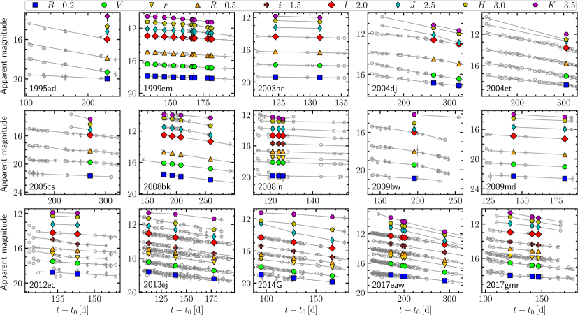
Figure 1: Light curves of the 15 SNe in the BC calibration sample. Colour-filled symbols correspond to the interpolated photometry, where bands and magnitude shifts with respect to the original values are indicated in the legend. Grey empty circles correspond to the photometry from the literature, and grey lines are the light-curve fits.

3.2 Quasi-bolometric correction

In the BC calibration sample, only 6 out of 15 SNe have $ri$ photometry. Therefore, we only use the $BV\!RI\!J\!H\!K$ photometry in order to compute quasi-bolometric fluxes with an homogeneous data set. We construct pSEDs and compute quasi-bolometric fluxes $F^{BV\!RI\!J\!H\!K}_{i}$ (in erg s^-1 cm^-2) using the prescription provided in Appendix B. We define the $x$-band quasi BC (qBC) as

$$\mathrm{qBC}_{x,i}=-2.5\log(F^{BV\!RI\!J\!H\!K}_{i})-m_{x,i}^{\mathrm{cor}},$$ (1)

where

$$m_{x,i}^{\mathrm{cor}}=m_{x,i}-R_{\bar{\lambda}_{x}}(E_{{B\!-\!V}}^{\mathrm{G}}+E_{{B\!-\!V}}^{\mathrm{h}}),$$ (2)

being $m_{x,i}$ the $x$-band magnitude at epoch $t_{i}$, and $R_{\bar{\lambda}_{x}}$ the total-to-selective extinction ratio for $\bar{\lambda}_{x}$, listed in Table 12.

3.3 Bolometric correction and luminosity

The flux from a pSED defined in a wavelength range $\lambda_{1}\text{\textendash}\lambda_{2}$ is only an approximation of the real flux computed integrating the SED in the same wavelength range, $F_{i}^{\lambda_{1}-\lambda_{2}}$. In our case, to quantify the relative difference between $F^{BV\!RI\!J\!H\!K}_{i}$ and $F_{i}^{\bar{\lambda}_{B}-\bar{\lambda}_{K}}$, we compute $\alpha_{i}$ such that

$$F_{i}^{\bar{\lambda}_{B}-\bar{\lambda}_{K}}=(1+\alpha_{i})F^{BV\!RI\!J\!H\!K}_{i}.$$ (3)

For this task we use the D13, J14, and L17 spectral models. To obtain $F^{BV\!RI\!J\!H\!K}_{i}$ from models, we first compute their synthetic magnitudes (see Appendix A) and then we compute $F^{BV\!RI\!J\!H\!K}_{i}$ with the recipe given in Appendix B.

Fig. 2 shows the $\alpha_{i}$ values computed with the three model sets. Since we do not find any correlation with colour indices, in the figure we plot $\alpha_{i}$ as a function of the time since explosion. For the D13, J14, and L17 models, the mean $\alpha$ values and their sample standard deviation ($\hat{\sigma}$) errors are ${-3.2\pm 1.8}$, ${4.6\pm 3.0}$, and ${1.1\pm 1.4}$ per cent, respectively. There is a difference of at least $2.6\,\hat{\sigma}$ between the mean $\alpha$ values from D13 and J14 models. Based on late-time optical spectra of 38 normal SNe II, Silverman et al. (2017) found that the J14 models fit better to the observations than the D13 ones. This evidence favour the scenario where $F_{i}^{\bar{\lambda}_{B}-\bar{\lambda}_{K}}$ is $\sim$5 per cent greater than $F^{BV\!RI\!J\!H\!K}_{i}$ instead of $\sim$3 per cent lower. To be conservative, we adopt the average of the mean $\alpha$ values of the three models, i.e., ${\alpha=0.8\pm 3.9}$ per cent ($1\,\hat{\sigma}$ error). This value is consistent within $\pm 1\,\hat{\sigma}$ with the results obtained for the three model sets.

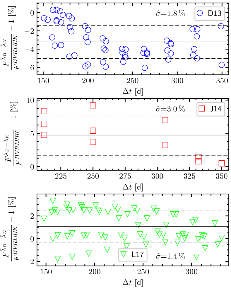
Figure 2: Relative differences between the flux computed with the pSED and the SED using the D13 (top panel), J14 (middle panel), and L17 (bottom panel) models. Solid and dashed lines correspond to mean values and $\pm 1\,\hat{\sigma}$ limits, respectively.

To compute the bolometric flux $F^{\mathrm{bol}}$, we have to correct $F^{\bar{\lambda}_{B}-\bar{\lambda}_{K}}$ for the unobserved flux. In our case,

$$F_{i}^{\mathrm{bol}}=F_{i}^{\bar{\lambda}_{B}-\bar{\lambda}_{K}}+F_{i}^{\lambda<\bar{\lambda}_{B}}+F_{i}^{\lambda>\bar{\lambda}_{K}},$$ (4)

where $F_{i}^{\lambda<\bar{\lambda}_{B}}$ and $F_{i}^{\lambda>\bar{\lambda}_{K}}$ are the unobserved fluxes at wavelengths below $\bar{\lambda}_{B}$ and beyond $\bar{\lambda}_{K}$, respectively.

For the unobserved flux below $\bar{\lambda}_{B}$, we write

$$F_{i}^{\lambda<\bar{\lambda}_{B}}=F_{i}^{\bar{\lambda}_{B}-\bar{\lambda}_{K}}c_{i}^{\lambda<\bar{\lambda}_{B}},$$ (5)

where

$$c_{i}^{\lambda<\bar{\lambda}_{B}}=F_{i}^{0.1\mu\mathrm{m}-\bar{\lambda}_{B}}/F_{i}^{\bar{\lambda}_{B}-\bar{\lambda}_{K}}$$ (6)

is the flux correction relative to $F_{i}^{\bar{\lambda}_{B}-\bar{\lambda}_{K}}$. We choose $0.1\,\micron$ as lower $\lambda$ value because it is the minimum wavelength in common for the three model sets. This value is also low enough to consider the flux negligible at shorter wavelengths.

Fig. 3(a) shows the $c_{i}^{\lambda<\bar{\lambda}_{B}}$ values as a function of ${B\!-\!V}$. As visible in the figure, there is a correlation between both quantities. The flux correction is lower than 2 per cent for ${{B\!-\!V}>1.7}$ and can be greater than 10 per cent for ${{B\!-\!V}<0.9}$. Within the colour range in common between the D13, J14, and L17 models (${1.0\leq{B\!-\!V}\leq 1.45}$), we see that values for the three model sets are in good agreement. We parametrize the dependence of $c_{i}^{\lambda<\bar{\lambda}_{B}}$ on ${B\!-\!V}$ as

$$c_{i}^{\lambda<\bar{\lambda}_{B}}=\sum_{j=0}^{2}\frac{a_{j}}{({B\!-\!V})_{i}^{j}},$$ (7)

where the quadratic order was determined using the model selection described in Appendix C. Table 1 lists the fit parameters along with the $\hat{\sigma}$ around the fit, which covers the colour range ${0.79\leq{B\!-\!V}\leq 2.02}$. Among the ${B\!-\!V}$ colours of the SNe in our BC calibration set (marked as magenta ticks in the figure), four are below the lower limit (two of SN 2014G, one of SN 1995ad, and one of SN 2004dj). In order to prevent a misestimation on $c_{i}^{\lambda<\bar{\lambda}_{B}}$ due to extrapolations, for ${B\!-\!V}$ colours bluer than 0.79 mag we adopt the $c^{\lambda<\bar{\lambda}_{B}}$ correction for ${{B\!-\!V}=0.79}$.

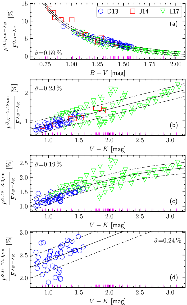
Figure 3: Corrections to account for the unobserved flux in the ranges $0.1\,\micron\text{\textendash}\bar{\lambda}_{B}$ (a), $\bar{\lambda}_{K}\text{\textendash}2.48\,\micron$ (b), $2.48\text{\textendash}3.0\,\micron$ (c), and $3.0\text{\textendash}75.9\,\micron$ (d), relative to the flux in the range $\bar{\lambda}_{B}\text{\textendash}\bar{\lambda}_{K}$, using the D13, J14, and L17 models. Magenta ticks mark the colours of the SNe in the BC calibration set. Solid lines indicate the fits to the models, while dashed lines are the $\pm 1\,\hat{\sigma}$ limits around the fit.

Table 1: Parameters for the flux corrections.

Correction	Colour	$a_{0}$ (%)	$a_{1}$ (%)	$a_{2}$ (%)	$\hat{\sigma}$ (%)
$\alpha$	–	$\phantom{-}0.80$	–	–	$3.90$
$c^{\lambda<\bar{\lambda}_{B}}$	${B\!-\!V}$	$-3.11$	$4.30$	$\phantom{-}6.72$	$0.59$
$c^{\bar{\lambda}_{K}-2.48\mu\mathrm{m}}$	${V\!-\!K}$	$\phantom{-}0.32$	$0.55$	–	$0.23$
$c^{2.48-3.0\mu\mathrm{m}}$	${V\!-\!K}$	$\phantom{-}0.31$	$1.09$	$-0.14$	$0.19$
$c^{\lambda>3\mu\mathrm{m}}$	${V\!-\!K}$	$\phantom{-}1.87$	$0.52$	–	$0.24$
$c^{\lambda>\bar{\lambda}_{K}}$	${V\!-\!K}$	$\phantom{-}2.50$	$2.16$	$-0.14$	$0.38$
Note: $c^{\lambda>\bar{\lambda}_{K}}=c^{\bar{\lambda}_{K}-2.48\mu\mathrm{m}}+c^{2.48-3.0\mu\mathrm{m}}+c^{\lambda>3\mu\mathrm{m}}$.

For the unobserved flux at $\lambda>\bar{\lambda}_{K}$ we use

$$F_{i}^{\lambda>\bar{\lambda}_{K}}=F_{i}^{\bar{\lambda}_{B}-\bar{\lambda}_{K}}c_{i}^{\lambda>\bar{\lambda}_{K}},$$ (8)

where, since the model sets do not cover the same wavelength range, we write

$$c_{i}^{\lambda>\bar{\lambda}_{K}}=c_{i}^{\bar{\lambda}_{K}-2.48\mu\mathrm{m}}+c_{i}^{2.48-3.0\mu\mathrm{m}}+c_{i}^{\lambda>3\mu\mathrm{m}},$$ (9)

being

$$c_{i}^{\bar{\lambda}_{K}-2.48\mu\mathrm{m}}=F_{i}^{\bar{\lambda}_{K}-2.48\mu\mathrm{m}}/F_{i}^{\bar{\lambda}_{B}-\bar{\lambda}_{K}},$$ (10)

$$c_{i}^{2.48-3.0\mu\mathrm{m}}=F_{i}^{2.48-3.0\mu\mathrm{m}}/F_{i}^{\bar{\lambda}_{B}-\bar{\lambda}_{K}},$$ (11)

and

$$c_{i}^{\lambda>3\mu\mathrm{m}}=F_{i}^{3.0-75.9\mu\mathrm{m}}/F_{i}^{\bar{\lambda}_{B}-\bar{\lambda}_{K}}.$$ (12)

Here, the values $2.48$ and $3.0\,\micron$ correspond to the maximum $\lambda$ in common for the {D13, J14, L17} and {D13, L17} model sets, respectively, while $75.9\,\micron$ is the maximum $\lambda$ for the D13 models.

Figs. 3(b) and 3(c) show $c_{i}^{\bar{\lambda}_{K}-2.48\mu\mathrm{m}}$ and $c_{i}^{2.48-3.0\mu\mathrm{m}}$, respectively, as a function of ${V\!-\!K}$. Those flux corrections, as expected, are greater for red colours than for blue ones. We express the dependence of $c_{i}^{\bar{\lambda}_{K}-2.48\mu\mathrm{m}}$ and $c_{i}^{2.48-3.0\mu\mathrm{m}}$ on ${V\!-\!K}$ through polynomials, i.e.,

$$c_{i}^{\lambda_{1}-\lambda_{2}}=\sum_{j=0}^{\mathcal{O}_{\lambda_{1},\lambda_{2}}}a_{j}({V\!-\!K})_{i}^{j},$$ (13)

being the orders $\mathcal{O}_{\lambda_{1},\lambda_{2}}$ determined with the model selection described in Appendix C. The fit parameter values are summarized in Table 1. As in the case of $c_{i}^{\lambda<\bar{\lambda}_{B}}$, we find a good agreement between models within the ranges in common.

Fig. 3(d) shows the $c_{i}^{\lambda>3\mu\mathrm{m}}$ values as a function of ${V\!-\!K}$, where only the D13 models provide spectral information for ${\lambda>3\,\mu\mathrm{m}}$. In this case the best fit is a straight-line, whose parameters are reported in Table 1. Since the D13 models do not cover all the ${V\!-\!K}$ colours of the SNe in the BC calibration set, the straight-line fit could introduce errors due to extrapolation. However, we find that $c_{i}^{\lambda>3\mu\mathrm{m}}$ at ${V\!-\!K}=3.1$ (the reddest colour in the BC calibration set) is only 1 per cent (in value) greater than the correction for the reddest colour in the D13 models (${V\!-\!K}=1.57$). Therefore, we adopt the linear parametrization of $c_{i}^{\lambda>3\mu\mathrm{m}}$ for all the ${V\!-\!K}$ colour range (${0.80\leq{V\!-\!K}\leq 3.15}$).

Based on equation (9), $c_{i}^{\lambda>\bar{\lambda}_{K}}$ is a polynomial given by equation (13), where the coefficients $a_{j}$ are the sum of those of $c_{i}^{\bar{\lambda}_{K}-2.48\mu\mathrm{m}}$, $c_{i}^{2.48-3.0\mu\mathrm{m}}$, and $c_{i}^{\lambda>3\mu\mathrm{m}}$. Parameters for $c_{i}^{\lambda>\bar{\lambda}_{K}}$ are given in Table 1.

Once $\alpha$, $c_{i}^{\lambda<\bar{\lambda}_{B}}$, and $c_{i}^{\lambda>\bar{\lambda}_{K}}$ are determined, we define the apparent bolometric magnitude and the $x$-band BC as

$$m_{\mathrm{bol},i}=-2.5\log(F^{BV\!RI\!J\!H\!K}_{i})-\kappa_{i}$$ (14)

and

$$\mathrm{BC}_{x,i}=m_{\mathrm{bol},i}-m_{x,i}^{\mathrm{cor}}=\mathrm{qBC}_{x,i}-\kappa_{i},$$ (15)

respectively. The model-based correction, $\kappa_{i}$, is given by

$$\kappa_{i}=2.5\log\left(1+\alpha\right)+2.5\log\left(1+c_{i}^{\lambda<\bar{\lambda}_{B}}+c_{i}^{\lambda>\bar{\lambda}_{K}}\right),$$ (16)

where the error in $\kappa_{i}$ is dominated by the error in $\alpha$ (see Table 1). For the SNe in the BC calibration set, the model-based correction ranges between 0.09 mag (SN 2005cs) and 0.22 mag (SN 2014G), with a median of 0.11 mag. Therefore, during the radioactive tail, the observed $F^{BV\!RI\!J\!H\!K}$ typically corresponds to 90 per cent of the bolometric flux.

Once $\mathrm{BC}_{x}$ values are calibrated with observations (section 4.2), luminosities ($L$, in $10^{43}\,\mathrm{erg\,s}^{-1}$) can be estimated through the BC technique, given by

$$\log{L_{i}}=(\mu-\mathrm{BC}_{x,i}-m_{x,i}^{\mathrm{cor}})/2.5-2.922,$$ (17)

where the constant provides the conversion from magnitude to cgs units.

3.4 ⁵⁶Ni Mass

During the radioactive tail, the energy sources powering the ejecta are the $\gamma$-rays and positrons produced in the radioactive decay of ⁵⁶Co into ⁵⁶Fe. The latter deposit energy in the ejecta at a rate $Q_{\mathrm{dep}}$. Using equations (10)–(12) of Wygoda et al. (2019), and assuming that the deposited energy is immediately emitted, we can write the relation between $Q_{\mathrm{dep}}$ (in $10^{43}\,\mathrm{erg\,s}^{-1}$) and $M_{{}^{56}\mathrm{Ni}}$ (in $\mathrm{M}_{\sun}$) as

$$\log Q_{\mathrm{dep},i}=\log M_{{}^{56}\mathrm{Ni}}-0.39\left[\frac{\Delta t_{i}}{100\,\mathrm{d}}\right]+0.154+D_{i}.$$ (18)

Here, $\Delta t_{i}=(t_{i}-t_{0})/(1+z^{\mathrm{SN}}_{\mathrm{helio}})$ is the time since explosion in the SN rest frame, and

$$D_{i}=\log(0.97f_{\mathrm{dep},i}+0.03),$$ (19)

where $f_{\mathrm{dep}}$ is the $\gamma$-ray deposition function, which describes the fraction of the generated $\gamma$-ray energy deposited in the ejecta. Knowing the deposition function, $\log M_{{}^{56}\mathrm{Ni}}$ can be inferred by equating equations (17) and (18).

If all the $\gamma$-ray energy is deposited in the ejecta, then ${f_{\mathrm{dep},i}=1}$ (${D_{i}=0}$), otherwise ${f_{\mathrm{dep},i}<1}$ (${D_{i}<0}$). In the first case, we expect the $\log M_{{}^{56}\mathrm{Ni}}$ estimates (one for each $\log{L_{i}}$ measurement) to be consistent with a constant value. In the second case, the $\log M_{{}^{56}\mathrm{Ni}}$ estimates decrease with time as the ejecta becomes less able to thermalize $\gamma$-rays (Section 4.3.1), which makes it necessary to correct for $f_{\mathrm{dep}}$. For the latter we adopt the model of Jeffery (1999):

$$f_{\mathrm{dep},i}=1-\exp{[-(T_{0}/\Delta t_{i})^{2}]},$$ (20)

where $T_{0}$ is a characteristic time-scale (in d) that represents the $\gamma$-ray escape time. This parameter is estimated such that the $\log M_{{}^{56}\mathrm{Ni}}$ estimates are consistent with a constant value.

To detect possible $\gamma$-ray leakage from the ejecta, we need at least three photometric points as we have to infer $T_{0}$ and $\log M_{{}^{56}\mathrm{Ni}}$. The detailed recipe to compute $\log M_{{}^{56}\mathrm{Ni}}$ and check if it is necessary to correct for $f_{\mathrm{dep}}$ is provided in Appendix D. In order to properly convert $\log M_{{}^{56}\mathrm{Ni}}$ into $M_{{}^{56}\mathrm{Ni}}$, we use the formalism provided in Appendix E.

3.5 Iron mass

The inferred $M_{{}^{56}\mathrm{Ni}}$ provides a good estimate of the ejected ⁵⁶Fe mass ($M_{{}^{56}\mathrm{Fe}}$). The $M_{\mathrm{Fe}}$ value, however, is greater than $M_{{}^{56}\mathrm{Fe}}$ since it is also composed of the stable isotopes ^54,57,58Fe (e.g. Curtis et al., 2019). Using the relation

$$\eta=M_{\mathrm{Fe}}/M_{{}^{56}\mathrm{Ni}}=1+M_{{}^{54,57,58}\mathrm{Fe}}/M_{{}^{56}\mathrm{Fe}}$$ (21)

and the CC nucleosynthesis yield models of Iwamoto et al. (1999), Blanc & Greggio (2008) computed ${\eta=1.08}$.

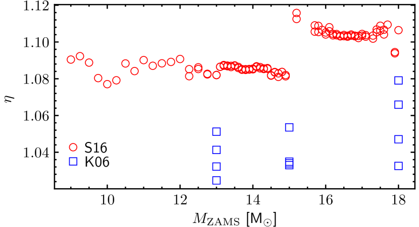
Figure 4: $M_{\mathrm{Fe}}/M_{{}^{56}\mathrm{Fe}}$ against $M_{\mathrm{ZAMS}}$. Blue squares and red circles correspond to K06 and S16 models, respectively.

Fig. 4 shows the $\eta$ values obtained with the K06 and S16 models. Since we do not find any correlation with model parameters, in the figure we plot $\eta$ against $M_{\mathrm{ZAMS}}$. The $\eta$ values range between 1.03 and 1.11, where the S16 values for ${M_{\mathrm{ZAMS}}\leq 15\,\mathrm{M}_{\sun}}$ are around 0.02 lower than those for ${M_{\mathrm{ZAMS}}>15\,\mathrm{M}_{\sun}}$. The $\eta$ values computed with the K06 models are up to 0.06 lower than those from S16 models. Since neither model is preferred, to be conservative we adopt ${\eta=1.07\pm 0.04}$ (the mid-point between 1.03 and 1.11, with the error being half the range). This value, consistent with that reported in Blanc & Greggio (2008), indicates that the measured $M_{{}^{56}\mathrm{Ni}}$ accounts to about 93 per cent of $M_{\mathrm{Fe}}$.

3.6 Host galaxy distance moduli and colour excesses

The error on $\log M_{{}^{56}\mathrm{Ni}}$ is mainly dominated by uncertainties on $\mu$ and $E_{{B\!-\!V}}^{\mathrm{h}}$ (e.g. Pejcha & Prieto, 2015b). To reduce their errors, we measure $\mu$ and $E_{{B\!-\!V}}^{\mathrm{h}}$ with various methods.

3.6.1 Distance moduli

To estimate $\mu$ for the SN host galaxies, we use distance moduli obtained with the Cepheids period-luminosity relation ($\mu_{\mathrm{CPL}}$), the Tip of the Red Giant Branch method ($\mu_{\mathrm{TRGB}}$), and the Tully-Fisher relation ($\mu_{\mathrm{TF}}$). We compile $\mu_{\mathrm{CPL}}$ and $\mu_{\mathrm{TRGB}}$ values from the literature, and $\mu_{\mathrm{TF}}$ from the Extragalactic Distance Database (EDD, Tully et al., 2009). If a host galaxy does not have $\mu_{\mathrm{CPL}}$ nor $\mu_{\mathrm{TRGB}}$, then we include distances (1) computed with the Hubble-Lemaître law ($D_{\mathrm{HLL}}$) using a local Hubble-Lemaître constant ($H_{0}$) of $74.03\pm 1.42$ km s^-1 Mpc^-1 (Riess et al., 2019) and including a velocity dispersion of 382 km s^-1 to account for the effect of peculiar velocities over $D_{\mathrm{HLL}}$; and (2) from distance-velocity calculators based on smoothed velocity fields ($D_{\mathrm{SVF}}$) given by Shaya et al. (2017) for ${D_{\mathrm{SVF}}<38}$ Mpc and Graziani et al. (2019) for ${D_{\mathrm{SVF}}<200}$ Mpc. These calculators are available on the EDD website⁵ and described in Kourkchi et al. (2020). Since the latter do not provide distance uncertainties, we adopt the typical distance error of the neighbouring galaxies as a conservative estimate, or a 15 per cent error if the host galaxy is isolated (Ehsan Kourkchi, private communication). We convert $D_{\mathrm{HLL}}$ ($D_{\mathrm{SVF}}$) into $\mu_{\mathrm{HLL}}$ ($\mu_{\mathrm{SVF}}$) using the recipe provided in Appendix E.

Table 16 summarizes the aforementioned distance moduli. From this compilation, we adopt as $\mu$ the weighted average of $\mu_{\mathrm{CPL}}$, $\mu_{\mathrm{TRGB}}$, and $\mu_{\mathrm{TF}}$, if the first ones are available, otherwise we adopt the weighted average of $\mu_{\mathrm{TF}}$, $\mu_{\mathrm{HLL}}$, and $\mu_{\mathrm{SVF}}$. In the case of SN 2006my, whose host galaxy is within the Virgo Cluster, we include the distance modulus reported in Foster et al. (2014) based on the planetary nebula luminosity function. The $\mu$ values are in Column 5 of Table 14. The typical $\mu$ error is of 0.18 mag.

3.6.2 Colour excesses

To calculate $E_{{B\!-\!V}}^{\mathrm{h}}$ we use the following methods:

• The colour-colour curve (C3) method (Rodríguez et al., 2014; Rodríguez et al., 2019). This technique assumes that, during the plateau phase, all normal SNe II have similar linear ${V\!-\!I}$ versus ${B\!-\!V}$ C3s. Under this assumption, the $E_{{B\!-\!V}}^{\mathrm{h}}$ value of an SN can be inferred from the vertical displacement of its observed C3 with respect to a reddening-free C3 (for a graphical representation, see Fig. 3 of Rodríguez et al. 2014). Using the C3 method (Appendix F), implemented in the C3M code, we measure the colour excesses ($E_{{B\!-\!V}}^{\mathrm{h,C3}}$) of 71 SNe in our set. Those values are reported in Column 2 of Table 17. The typical $E_{{B\!-\!V}}^{\mathrm{h,C3}}$ uncertainty is of 0.085 mag.

• The colour method (e.g. Olivares E. et al., 2010). This technique assumes that all normal SNe II have the same intrinsic ${V\!-\!I}$ colour at the end of the plateau phase. Olivares E. et al. (2010) defined this epoch as 30 d before the middle of the $V$-band transition phase ($t_{\mathrm{PT},V}$, see Section 4.5). The prescription provided by Olivares E. et al. (2010) to compute colour excesses can be written as

  $$E_{{B\!-\!V}}^{\mathrm{h},{V\!-\!I}}=0.812[({V\!-\!I})_{-30}-0.656],$$ (22)

  $$\sigma_{E_{{B\!-\!V}}^{\mathrm{h},{V\!-\!I}}}=0.812\sqrt{\sigma_{({V\!-\!I})_{-30}}^{2}+0.079^{2}}.$$ (23)

  Here, $({V\!-\!I})_{-30}$ is the ${V\!-\!I}$ colour measured at $t_{\mathrm{PT},V}-30$ d corrected for $E_{{B\!-\!V}}^{\mathrm{G}}$ and $K$-correction (e.g. Rodríguez et al. 2019). We compute $E_{{B\!-\!V}}^{\mathrm{h},{V\!-\!I}}$ values for 59 SNe in our sample. For SNe 2012aw and 2013am we adopt the values provided in the literature. Column 3 of Table 17 lists the $E_{{B\!-\!V}}^{\mathrm{h},{V\!-\!I}}$ values, which have a typical uncertainty of 0.074 mag.

• Spectrum-fitting method (e.g. Dessart et al., 2008; Olivares E. et al., 2010). This technique consists on inferring the colour excess ($E_{{B\!-\!V}}^{\mathrm{h,spec}}$) of an SN from the comparison between its spectra and those of reddening-corrected SNe or spectral models. We compile $E_{{B\!-\!V}}^{\mathrm{h,spec}}$ values from the literature for 22 SNe in our set. We also compute $E_{{B\!-\!V}}^{\mathrm{h,spec}}$ for 36 SNe in our sample, using the prescription given in Appendix G. The $E_{{B\!-\!V}}^{\mathrm{h,spec}}$ are collected in Column 4 of Table 17. The typical $E_{{B\!-\!V}}^{\mathrm{h,spec}}$ uncertainty is of 0.091 mag.

Fig 5 shows residuals about the one-to-one relation between $E_{{B\!-\!V}}^{\mathrm{h,C3}}$ and $E_{{B\!-\!V}}^{\mathrm{h},{V\!-\!I}}$ ($r^{\mathrm{C3}}_{V\!-\!I}$, top panel), $E_{{B\!-\!V}}^{\mathrm{h},{V\!-\!I}}$ and $E_{{B\!-\!V}}^{\mathrm{h,spec}}$ ($r^{V\!-\!I}_{\mathrm{spec}}$, middle panel), and between $E_{{B\!-\!V}}^{\mathrm{h,spec}}$ and $E_{{B\!-\!V}}^{\mathrm{h,C3}}$ ($r^{\mathrm{spec}}_{\mathrm{C3}}$, bottom panel) for the 44 SNe in our set having $E_{{B\!-\!V}}^{\mathrm{h,C3}}$, $E_{{B\!-\!V}}^{\mathrm{h},{V\!-\!I}}$, and $E_{{B\!-\!V}}^{\mathrm{h,spec}}$. For $r^{\mathrm{C3}}_{V\!-\!I}$ we obtain a mean, $\hat{\sigma}$, and typical error of 0.02, 0.09, and 0.10 mag, respectively. For $r^{V\!-\!I}_{\mathrm{spec}}$ we compute a mean, $\hat{\sigma}$, and typical error of 0.00, 0.14, and 0.12 mag, respectively. For $r^{\mathrm{spec}}_{\mathrm{C3}}$ we calculate a mean, $\hat{\sigma}$, and typical error of $-0.02$, 0.13, and 0.12 mag, respectively. Since the $\hat{\sigma}$ values are quite similar to the typical residual errors, the observed dispersion is mainly due to colour excess errors. The mean offsets are statistically consistent with zero within $\pm 1.3\hat{\sigma}/\sqrt{N}$. Therefore, we do not detect systematic differences between the colour excesses inferred with the three aforementioned methods. Based on the latter, for the 77 SNe in our set having $E_{{B\!-\!V}}^{\mathrm{h,C3}}$, $E_{{B\!-\!V}}^{\mathrm{h},{V\!-\!I}}$, and/or $E_{{B\!-\!V}}^{\mathrm{h,spec}}$ estimates, we adopt the weighted mean of those values as $E_{{B\!-\!V}}^{\mathrm{h}}$. For SNe 1980K, 2006my, 2008gz, 2014cx, and 2017it we obtain negative $E_{{B\!-\!V}}^{\mathrm{h}}$ values (see Column 6 of Table 14). The values of the first four objects are consistent with zero within $1.3\,\sigma$, while for SN 2017it the offset is of $-2.1\,\sigma$. Although negative $E_{{B\!-\!V}}^{\mathrm{h}}$ values have no physical meaning, we keep those values as we do not have evidence to discard them.

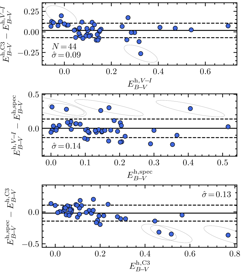
Figure 5: Residuals about the one-to-one relation between $E_{{B\!-\!V}}^{\mathrm{h}}$ values computed with the C3 method and the colour method (top panel), the colour method and the spectrum-fitting technique (middle panel), and the spectrum-fitting technique and the C3 method (bottom panel). Solid lines are mean values and dashed lines are $\pm 1\,\hat{\sigma}$ limits. Ellipses are $1\,\sigma$ confidence regions, which for clarity are drawn only for SNe outside $\pm 2\,\hat{\sigma}$ from the mean.

For SNe in out sample without $E_{{B\!-\!V}}^{\mathrm{h}}$ estimates, we evaluate to use colour excesses inferred from the pseudo-equivalent width of the host galaxy Na i D absorption line ($\mathrm{pEW_{NaID}}$). We compile $\mathrm{pEW_{NaID}}$ values from the literature for 89 SNe in our sample. With those values, we compute colour excesses ($E_{{B\!-\!V}}^{\mathrm{h,NaID}}$) using the relation of Poznanski et al. (2012), and adopting a relative $E_{{B\!-\!V}}$ error of 68 per cent (Phillips et al., 2013). The $\mathrm{pEW_{NaID}}$ becomes insensitive to estimate the colour excess for $\mathrm{pEW_{NaID}}>0.1$ nm (e.g. Phillips et al., 2013), equivalent to ${E_{B\!-\!V}>0.21\pm 0.14}$ mag in the Poznanski et al. (2012) relation. Therefore, we assume the latter lower limit for all SNe with $\mathrm{pEW_{NaID}}$ greater than 0.1 nm. The $E_{{B\!-\!V}}^{\mathrm{h,NaID}}$ values are listed in Column 4 of Table 17.

Fig 6(a) shows $E_{{B\!-\!V}}^{\mathrm{h,NaID}}$ against $E_{{B\!-\!V}}^{\mathrm{h}}$ (54 SNe). Fitting a straight line with a slope of unity, we measure an offset and $\hat{\sigma}$ value of $-0.09$ and 0.11 mag, respectively. The offset is equivalent to $-6.0\,\hat{\sigma}/\sqrt{N}$, which means that the $E_{{B\!-\!V}}^{\mathrm{h,NaID}}$ values are systematically lower than $E_{{B\!-\!V}}^{\mathrm{h}}$. Therefore, for the 24 SNe in our sample without $E_{{B\!-\!V}}^{\mathrm{h}}$ estimates but with $E_{{B\!-\!V}}^{\mathrm{h,NaID}}$ values we adopt ${E_{{B\!-\!V}}^{\mathrm{h}}=E_{{B\!-\!V}}^{\mathrm{h,NaID}}+0.09}$ mag, including in quadrature an error of 0.11 mag.

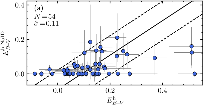
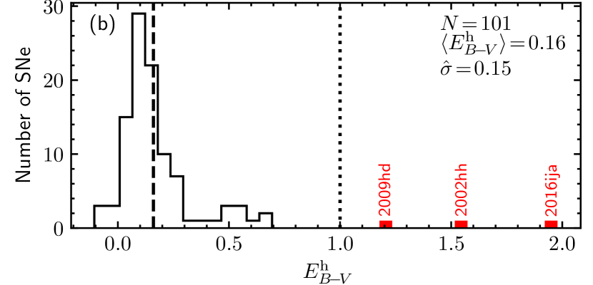
Figure 6: Panel (a): colour excesses computed from $\mathrm{pEW_{NaID}}$ versus the $E_{{B\!-\!V}}^{\mathrm{h}}$ values adopted in this work. The solid line is a straight line fit with a slope of unity, and dashed lines are the $\pm 1\,\hat{\sigma}$ limits around the fit. Error bars are $1\,\sigma$ errors. Panel (b): histogram of $E_{{B\!-\!V}}^{\mathrm{h}}$. The dotted line is the Chauvenet upper rejection limit ($E_{{B\!-\!V}}^{\mathrm{h}}=1$ mag). The dashed line indicates the mean $E_{{B\!-\!V}}^{\mathrm{h}}$ of the 101 SNe with $E_{{B\!-\!V}}^{\mathrm{h}}<1$ mag. Red bins are outliers.

For the highly reddened SNe 2002hh and 2016ija (both without $E_{{B\!-\!V}}^{\mathrm{h}}$ and with ${E_{{B\!-\!V}}^{\mathrm{h,NaID}}>0.21}$ mag) we adopt the $E_{{B\!-\!V}}^{\mathrm{h}}$ values reported by Pozzo et al. (2006) and Tartaglia et al. (2018), respectively. In the case of SN 2002hh, the colour excess has two components: ${E_{{B\!-\!V}}=1.065}$ mag (which includes $E_{{B\!-\!V}}^{\mathrm{G}}$) with ${R_{V}=3.1}$, and ${E_{{B\!-\!V}}=1.545\pm 0.182}$ mag with ${R_{V}=1.1}$. For simplicity in the forthcoming analyses, we consider the first component as $E_{{B\!-\!V}}^{\mathrm{G}}$ and the second one as $E_{{B\!-\!V}}^{\mathrm{h}}$.

Fig. 6(b) shows the histogram of $E_{{B\!-\!V}}^{\mathrm{h}}$. To identify extreme values in the $E_{{B\!-\!V}}^{\mathrm{h}}$ distribution, we use the Chauvenet (1863) criterion. We find that SNe 2002hh, 2009hd, and 2016ija have $E_{{B\!-\!V}}^{\mathrm{h}}$ values greater than the Chauvenet upper rejection limit ($E_{{B\!-\!V}}^{\mathrm{h}}=1$ mag), so we consider them as outliers. The $E_{{B\!-\!V}}^{\mathrm{h}}$ distribution (removing the extreme values) has a mean and $\hat{\sigma}$ of 0.16 and 0.15 mag, respectively. For the six SNe in our set without $E_{{B\!-\!V}}^{\mathrm{h}}$ (SNe 2004eg, PTF11go, PTF11htj, PTF11izt, PTF12grj, and LSQ13dpa) we adopt the mean and $\hat{\sigma}$ of the latter distribution as $E_{{B\!-\!V}}^{\mathrm{h}}$ and its error, respectively.

The adopted $E_{{B\!-\!V}}^{\mathrm{h}}$ values are in Column 6 of Table 14. The typical $E_{{B\!-\!V}}^{\mathrm{h}}$ error is of 0.08 mag.

3.7 Explosion epochs

The SN explosion epoch is typically estimated as the midpoint between the last non-detection $t_{\mathrm{ln}}$ and the first SN detection $t_{\mathrm{fd}}$. In order to improve the $t_{0}$ estimates for the SNe in our set, we use the SNII_ETOS code (Rodríguez et al., 2019). The latter computes $t_{0}$ given a set of optical spectra as input and a uniform prior on $t_{0}$ provided by $t_{\mathrm{ln}}$ and $t_{\mathrm{fd}}$ (for more details, see Rodríguez et al. 2019). If SNII_ETOS is not able to compute $t_{0}$ for an SN, then we adopt the midpoint between $t_{\mathrm{ln}}$ and $t_{\mathrm{fd}}$ if ${t_{\mathrm{fd}}-t_{\mathrm{ln}}<20}$ d, otherwise we use the $t_{0}$ value reported in the literature.

Table 18 lists the $t_{\mathrm{ln}}$ (Column 2), $t_{\mathrm{fd}}$ (Column 3), and the adopted $t_{0}$ (Column 4) values (also reported in Column 7 of Table 14) for our SN set. The typical $t_{0}$ error is of 3.8 d.

4 Analysis

4.1 Quasi-bolometric and bolometric corrections

The top panel of Fig. 7 shows the $\mathrm{qBC}_{V}$ values for the 15 SNe in the BC calibration set against the time since explosion. For comparison we include the D13, J14, and L17 models, along with the long-rising SN 1987A, which is typically used to estimate $\mathrm{BC}_{V}$ for normal SNe II (e.g. Hamuy, 2001; Bersten & Hamuy, 2009; Maguire et al., 2010). In the figure we see that, except for SN 2014G, the four SNe with three or more points at ${\Delta t<250}$ d and a time baseline greater than 30 d (SNe 1999em, 2008bk, 2013ej, and 2017eaw) seems to be consistent with a constant $\mathrm{qBC}_{V}$ value, as in the case of SN 1987A. For SNe 2017eaw and 2008bk we notice that the $\mathrm{qBC}_{V}$ values at ${\Delta t>250}$ d are $0.1$–$0.15$ mag greater than the values at ${\Delta t<210}$ d. This could be due to the effect of newly formed dust. We also notice differences in $\mathrm{qBC}_{V}$ of around $0.3\text{\textendash}0.7$ mag between the sub-luminous SNe 2005cs, 2008bk, 2009md (e.g. Spiro et al., 2014) and the moderately-luminous SNe 2004et and 2009bw (e.g. Inserra et al., 2013).

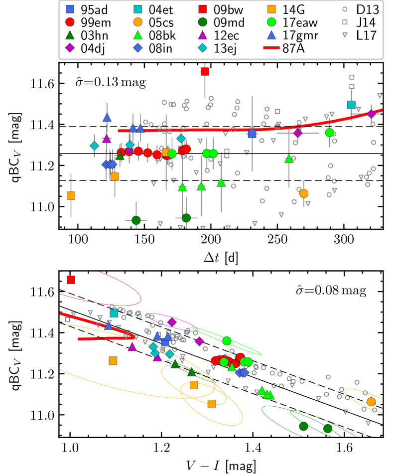
Figure 7: q$\mathrm{BC}_{V}$ values for the SNe in the BC calibration set (filled symbols), the D13, J14, and L17 models (empty symbols), and the long-rising SN 1987A (red thick line), as a function of time since explosion (top panel) and ${V\!-\!I}$ colour (bottom panel). Solid lines are the best polynomial fit to the observed data, while dashed lines indicate the $\pm 1\,\hat{\sigma}$ limits around the fit. Error bars are $1\,\sigma$ errors and ellipses indicate $1\,\sigma$ confidence regions, which for clarity are drawn only for SNe outside the $\pm 1\,\hat{\sigma}$ limits.

The bottom panel of Fig. 7 shows $\mathrm{qBC}_{V}$ versus ${V\!-\!I}$. We detect a correlation between both quantities, in the sense that the redder the SN the lower the $\mathrm{qBC}_{V}$. This correlation is also displayed by models (empty symbols), which are consistent with the linear fit to the observations (solid line) within $\pm 1\,\hat{\sigma}$ (dashed lines). Since the errors in $E_{{B\!-\!V}}^{\mathrm{h}}$, $E_{{B\!-\!V}}^{\mathrm{G}}$, and $V$-band photometry affect the $\mathrm{qBC}_{V}$ and ${V\!-\!I}$ values, the confidence region of each observation is an elongated ellipse. We see that the confidence regions are nearly oriented in the direction of the $\mathrm{qBC}_{V}$ versus ${V\!-\!I}$ correlation. Therefore, the errors in $E_{{B\!-\!V}}^{\mathrm{G}}$, $E_{{B\!-\!V}}^{\mathrm{h}}$, and $V$-band photometry are not the main sources of the observed dispersion.

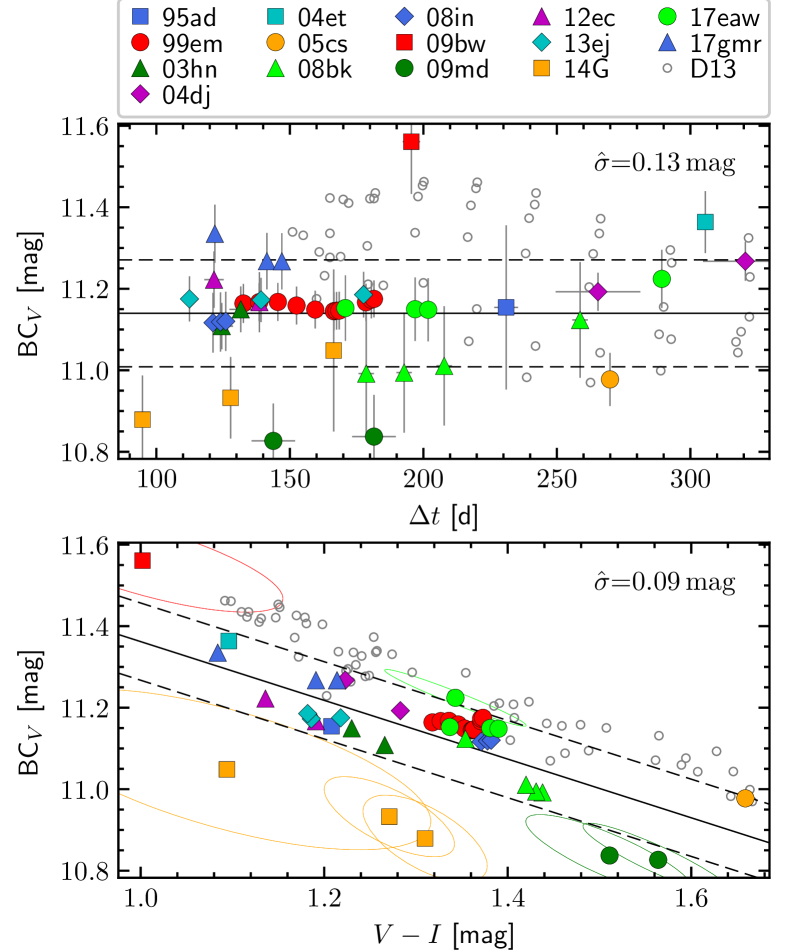
Figure 8: $\mathrm{BC}_{V}$ values as a function of time since explosion (top panel) and ${V\!-\!I}$ (bottom panel). Symbols, lines, error bars, and ellipses have the same meaning than in Fig. 7.

Fig. 8 shows $\mathrm{BC}_{V}$ against the time since explosion (top panel) and ${V\!-\!I}$ (bottom panel). As we can see in the figure, the behaviour of $\mathrm{BC}_{V}$ is the same as that of $\mathrm{qBC}_{V}$.

4.2 BC calibration

4.2.1 $\mathrm{BC}_{V}$ versus ${V\!-\!I}$

To calibrate the dependence of $\mathrm{BC}_{V}$ on ${V\!-\!I}$ displayed in the bottom panel of Fig. 8, we use the expression

$$\mathrm{BC}_{x}=\mathrm{ZP}_{x}^{\mathrm{BC}}+\Psi_{x}(X).$$ (24)

Here, $\mathrm{ZP}_{x}^{\mathrm{BC}}$ is the zero-point for the $x$-band BC calibration, and $\Psi_{x}$ is a polynomial function (without the zero-order term) representing the dependence of $\mathrm{BC}_{x}$ on the independent variable $X$ (in our case, ${X={V\!-\!I}}$). To compute the polynomial parameters, we minimize

$$s^{2}=\sum_{\mathrm{SN}}\sum_{i}\left[\mathrm{BC}_{V,i}^{\mathrm{SN}}+\delta^{\mathrm{SN}}-\Psi_{V}\left(({V\!-\!I})_{i}^{\mathrm{SN}}\right)\right]^{2},$$ (25)

where $\delta^{\mathrm{SN}}$ is an additive term to normalize the $\mathrm{BC}_{V}$ values of each SN to the same scale, and the polynomial order is determined with the model selection described in Appendix C.

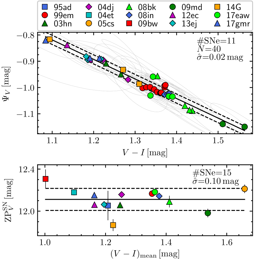
Figure 9: Top panel: $\Psi_{V}$ against ${V\!-\!I}$, where the solid line is a linear fit and ellipses are the $1\,\sigma$ confidence regions. Bottom panel: $\mathrm{ZP}^{\mathrm{SN}}_{V}$ as a function of the mean ${V\!-\!I}$ colour, where the solid line indicates the mean value. Dashed lines are the $\pm 1\,\hat{\sigma}$ limits.

The top panel of Fig. 9 shows the result of the aforementioned process, where we exclude SNe 1995ad, 2004et, 2005cs, and 2009bw because they have only one $\mathrm{BC}_{V}$ estimate. From this analysis we obtain that data are well represented by a straight line with slope ($\beta_{V}$) of ${-0.745\pm 0.002}$.

To compute the $\mathrm{ZP}_{V}^{\mathrm{BC}}$ value for each SN ($\mathrm{ZP}_{V}^{\mathrm{SN}}$), we arrange equations (24), (15), and (2), obtaining

$$\mathrm{ZP}_{V}^{\mathrm{SN}}=\langle m_{\mathrm{bol},i}-(1+\beta_{V})V_{i}+\beta_{V}I_{i}\rangle+(E_{{B\!-\!V}}^{\mathrm{G}}+E_{{B\!-\!V}}^{\mathrm{h}})\xi,$$ (26)

where ${\xi=(1+\beta_{V})R_{\bar{\lambda}_{V}}-\beta_{V}R_{\bar{\lambda}_{I}}=2.01}$ (using the $R_{\bar{\lambda}_{x}}$ values provided in Table 12). The angle brackets in equation (26) denote a weighted mean with weights

$$w_{i}=\left[\sigma_{m_{\mathrm{bol},i}}^{2}+(1+\beta_{V})^{2}\sigma_{V_{i}}^{2}+\beta_{V}^{2}\sigma_{I_{i}}^{2}\right]^{-1},$$ (27)

where $\sigma_{m_{\mathrm{bol},i}}$ only includes the error on photometry. The random error for each $\mathrm{ZP}_{V}^{\mathrm{SN}}$ value is given by

$$\sigma_{\mathrm{ZP}_{V}^{\mathrm{SN}}}=\left[\frac{1}{\sum_{i}w_{i}}+(\sigma_{E_{{B\!-\!V}}^{\mathrm{G}}}^{2}+\sigma_{E_{{B\!-\!V}}^{\mathrm{h}}}^{2})\zeta^{2}\right]^{1/2},$$ (28)

where ${\zeta=\xi-R_{\mathrm{p}}}$, being $R_{\mathrm{p}}$ the pSED total-to-selective extinction ratio (see Appendix B). For our BC calibration set ${R_{\mathrm{p}}=1.68}$, so the $E_{{B\!-\!V}}^{\mathrm{G}}$ and $E_{{B\!-\!V}}^{\mathrm{h}}$ errors are scaled by 0.33. For example, an $E_{{B\!-\!V}}^{\mathrm{h}}$ uncertainty of 0.08 mag (the typical value for our sample) induces an error on $\mathrm{ZP}_{V}^{\mathrm{SN}}$ of 0.03 mag.

The bottom panel of Fig. 9 shows the $\mathrm{ZP}^{\mathrm{SN}}_{V}$ values for the SNe in the BC calibration set. To verify whether a residual correlation between $\mathrm{ZP}^{\mathrm{SN}}_{V}$ and ${V\!-\!I}$ exists, in the figure we plot the $\mathrm{ZP}^{\mathrm{SN}}_{V}$ values against mean ${V\!-\!I}$ colours. Using the model selection given in Appendix C, we find that data are consistent with $\mathrm{ZP}^{\mathrm{SN}}_{V}$ being constant, meaning that all the dependence of $\mathrm{ZP}^{\mathrm{SN}}_{V}$ on ${V\!-\!I}$ was captured by $\Psi_{V}$. We compute a mean and $\hat{\sigma}$ value of 12.11 and 0.10 mag, respectively. The typical $\mathrm{ZP}^{\mathrm{SN}}_{V}$ error is about $0.03$ mag, so the observed $\hat{\sigma}$ value is mainly due to intrinsic differences between SNe. Therefore we adopt ${\mathrm{ZP}_{V}^{\mathrm{BC}}=12.11\pm 0.10}$ mag.

4.2.2 BCs for other combinations

In addition to $\mathrm{BC}_{V}$ as a function of ${V\!-\!I}$, we also calibrate the dependence of $\mathrm{BC}_{x}$ for the $V\!r\!RiI$ bands as a function of different independent variables. In the BC calibration set there are only six SNe having $ri$ photometry in the radioactive tail (namely SNe 2008in, 2012ec, 2013ej, 2014G, 2017eaw, and 2017gmr). For the remaining nine SNe we convert the $RI$ magnitudes to $ri$ ones (see Appendix H).

To calibrate the dependence of $\mathrm{BC}_{x}$ on a given $X$ variable, we perform the same analysis as in Section 4.2.1. As independent variables, we consider the ten colour indices that can be defined with the $V\!r\!RiI$ bands along with $\Delta t$. We find that the BC calibrations providing the lowest $\hat{\sigma}$ values are $\mathrm{BC}_{V}$ as a function of ${V\!-\!I}$, $\mathrm{BC}_{r}$ as a function of $r\!-\!I$, $\mathrm{BC}_{R}$ as a function of $R\!-\!I$, $\mathrm{BC}_{i}$ as a function of $i\!-\!I$, and $\mathrm{BC}_{I}$ as a function of $\Delta t$. In all cases the dependence of $\mathrm{BC}_{x}$ on the $X$ variable is linear. The slopes of the linear relations ($\beta_{x}$) are reported in Column 3 of Table 2.

Table 2: BC calibrations.

$x$	$X$	$\beta_{x}$	$\mathrm{ZP}_{x}^{\mathrm{BC}}$ (mag)
$V$	${V\!-\!I}$	$-0.745\pm 0.002$	$12.11\pm 0.10$
$r$	$r\!-\!I$	$-0.837\pm 0.004$	$12.35\pm 0.10$
$R$	$R\!-\!I$	$-0.755\pm 0.007$	$12.35\pm 0.10$
$i$	$i\!-\!I$	$-0.963\pm 0.005$	$12.42\pm 0.10$
$I$	$\Delta t/(100\,\mathrm{d})$	$\phantom{-}0.036\pm 0.002$	$12.37\pm 0.10$
$V$	–	–	$11.15\pm 0.18$
$r$	–	–	$11.89\pm 0.16$
$R$	–	–	$12.07\pm 0.14$
$i$	–	–	$11.91\pm 0.12$
$I$	–	–	$12.44\pm 0.11$
Notes. $\mathrm{BC}_{x}=\mathrm{ZP}_{x}^{\mathrm{BC}}+\beta_{x}X$, valid for $\Delta t$ between 95 and 320 d. $\mathrm{ZP}_{x}^{\mathrm{BC}}$ errors do not include the uncertainty due to the $\alpha$ error.

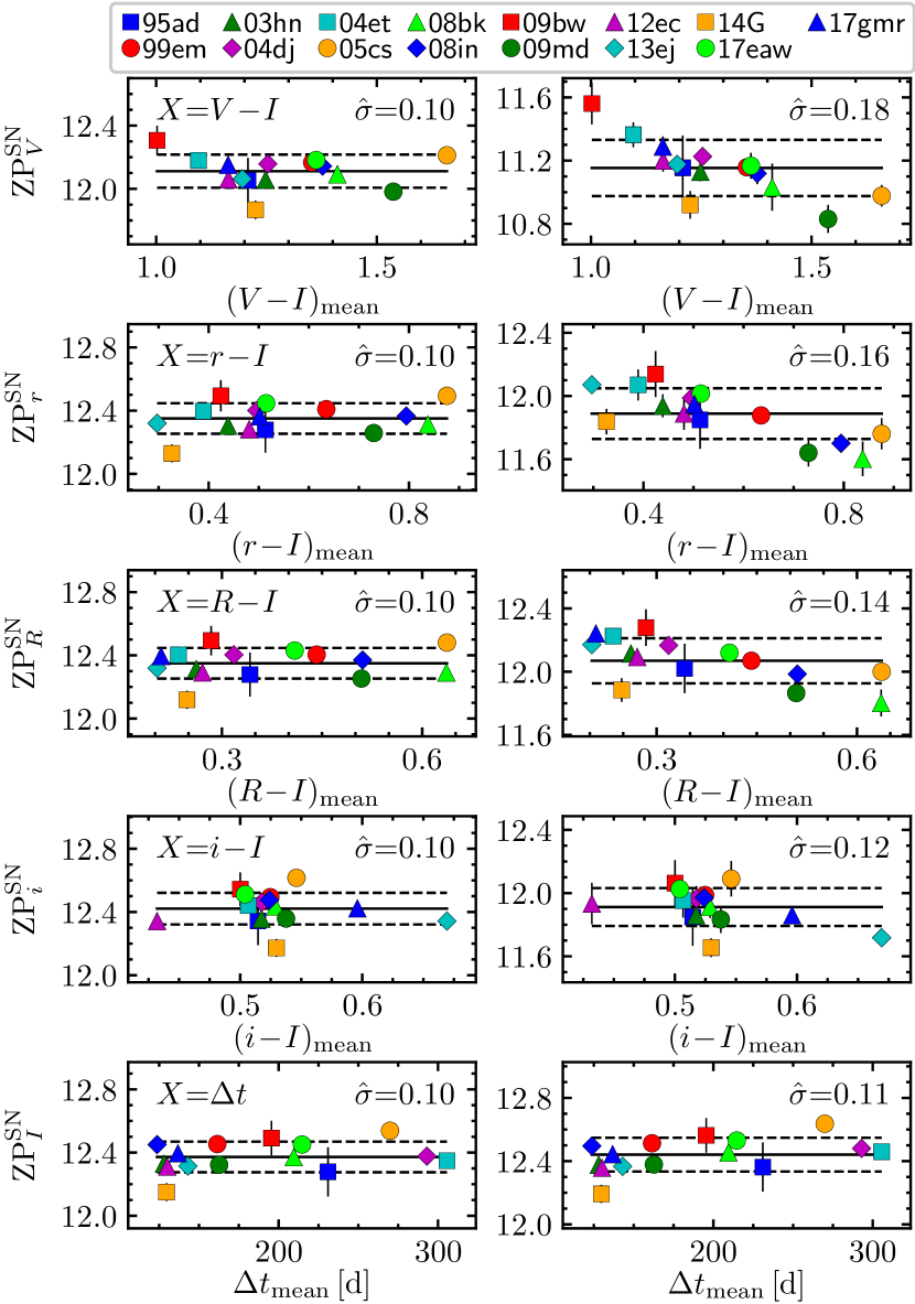
Figure 10: $\mathrm{ZP}^{\mathrm{SN}}_{x}$ versus the mean $X$ value. Left-hand panels: using the calibration with the lowest $\hat{\sigma}$ value. Right-hand panels: assuming a constant BC. Solid and dashed lines indicate mean values and $\pm 1\,\hat{\sigma}$ limits around the mean, respectively.

The left-hand side of Fig. 10 shows the $\mathrm{ZP}^{\mathrm{SN}}_{x}$ values for the aforementioned calibrations. For each one we find that the $\mathrm{ZP}^{\mathrm{SN}}_{x}$ estimates are consistent with a constant value (using the model selection given in Appendix C). As for $\mathrm{BC}_{V}$ as a function of ${V\!-\!I}$, for $r\!RiI$ bands we adopt the mean and $\hat{\sigma}$ value as $\mathrm{ZP}_{x}^{\mathrm{BC}}$ and its error, respectively. Those values are listed in Column 4 of Table 2. Given the domain of the data (top panel of Fig. 7), our BC calibrations are valid for $\Delta t$ between 95 and 320 d. Since the BC calibration set includes sub-luminous (SNe 2005cs, 2008bk, and 2009md) and moderately-luminous (e.g. SNe 2004et, 2009bw, and 2017gmr) SNe II, we assume that our $\mathrm{BC}_{x}$ calibrations are valid for all normal SNe II.

We also compute $\mathrm{BC}_{x}$ calibrations assuming they are constant. The $\mathrm{ZP}_{x}^{\mathrm{BC}}$ values are given in Column 4 of Table 2, while the $\mathrm{ZP}^{\mathrm{SN}}_{x}$ estimates are shown in the right-hand side of Fig. 10. Since $\mathrm{BC}_{x}$ is not actually constant but depends on a specific $X$ variable, there is a dependence of $\mathrm{ZP}^{\mathrm{SN}}_{x}$ on the mean $X$ values. The latter, as we can see in right-hand side of Fig. 10, is more evident for $V\!r\!R$ bands.

The BCs with the best precision are those including the $I$-band in the calibration (${\hat{\sigma}=0.10}$–0.11 mag), followed by $\mathrm{BC}_{i}$ as a constant (${\hat{\sigma}=0.12}$ mag). The latter means that, among the $V\!r\!RiI$ bands, the $I$- and $i$-band magnitudes are more correlated with the bolometric one. In order to compute luminosities through the BC technique (equation 17), the $I$-band photometry along with $\mathrm{BC}_{I}$ as a function of $\Delta t$ must be preferred. If the $I$-band photometry is not available, then the $i$-, $R$-, $r$-, or $V$-band photometry along with the constant $\mathrm{BC}_{x}$ can be used to estimate luminosities. In the latter case, however, we caution that the derived luminosities of sub-luminous and moderately-luminous SNe II will be systematically under and overestimated, respectively, specially for the $V\!r\!R$ bands.

4.3 ⁵⁶Ni mass distribution

4.3.1 $\log M_{{}^{56}\mathrm{Ni}}$ estimates

Armed with BCs for normal SNe II in the radioactive tail, we compute $\log M_{{}^{56}\mathrm{Ni}}$ using the recipe given in Appendix D.

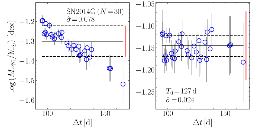
Figure 11: $\log M_{{}^{56}\mathrm{Ni}}$ estimates of SN 2014G versus the time since explosion, assuming the complete $\gamma$-ray trapping scenario (left-hand panel), and correcting for $f_{\mathrm{dep}}$ (right-hand panel). Solid horizontal lines correspond to the $\log M_{{}^{56}\mathrm{Ni}}$ values that maximize the likelihood, and dashed lines are the $\pm 1\,\hat{\sigma}$ limits around them. Error bars are $1\,\sigma$ errors due to uncertainties on photometry, while red vertical bars depict the $1\,\sigma$ errors due to the uncertainty on $\mu$, colour excesses, $t_{0}$, and BC.

For 25 SNe in our sample we find it is necessary to correct for the deposition function. As example, the left-hand side of Fig. 11 shows the $\log M_{{}^{56}\mathrm{Ni}}$ estimates of SN 2014G as a function of the time since explosion, assuming the complete $\gamma$-ray trapping scenario (i.e. $D_{i}=0$ in equation 18). As visible in the figure, the $\log M_{{}^{56}\mathrm{Ni}}$ estimates are not concentrated around a constant but they decrease with time. This trend emerges because the ejecta becomes less able to thermalize $\gamma$-rays with time. In this case of $\gamma$-ray leakage, the inferred $\log M_{{}^{56}\mathrm{Ni}}$ corresponds to a lower limit. The right-hand side of the figure shows the $\log M_{{}^{56}\mathrm{Ni}}$ estimates corrected for $f_{\mathrm{dep}}$. We can see that, using $T_{0}=127$ d, the systematic with time disappears and the $\log M_{{}^{56}\mathrm{Ni}}$ estimates are consistent with a constant value.

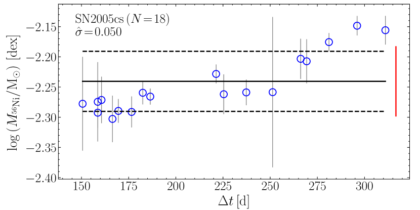
Figure 12: $\log M_{{}^{56}\mathrm{Ni}}$ estimates of SN 2005cs versus the time since explosion, assuming the complete $\gamma$-ray trapping scenario. Error bars and lines have the same meaning than in Fig. 11.

In our SN set, SNe 2004dj, 2005cs, 2006my, 2013am, and 2013bu have $\log M_{{}^{56}\mathrm{Ni}}$ estimates that increase with time, which is shown in Fig. 12 for the case of SN 2005cs. This trend indicates that the observed luminosity increases with time relative to that expected from the radioactive decay. The latter suggests that (1) the SN ejecta during the early radioactive tail is not optically thin enough, so the energy deposited in the ejecta is not immediately emitted (i.e. ${L<Q_{\mathrm{dep}}}$); and/or (2) there is an additional source of energy (i.e. ${L>Q_{\mathrm{dep}}}$), whose relative contribution to the observed flux increases with time. For the latter scenarios, the higher and lower $\log M_{{}^{56}\mathrm{Ni}}$ estimates are closer to the real value, respectively. In this work, in order to be conservative about the origin of the observed tendency, for the aforementioned five SNe we adopt the $\log M_{{}^{56}\mathrm{Ni}}$ value obtained with ${D_{i}=0}$.

In the case of SNe 1988A, 2003iq, 2005dx, PTF10gva, 2010aj, LS13dpa, 2015cz, and 2016ija we obtain ${D_{i}=0}$ because the characteristics of their photometry (number of data, photometry errors, and time baseline) are not good enough to detect departures from a constant $\log M_{{}^{56}\mathrm{Ni}}$ value. In our sample 30 out of 102 SNe are consistent with ${D_{i}\neq 0}$. Therefore, we expect only two out of the aforementioned SNe to have ${D_{i}\neq 0}$, which should not impact our results.

Table 19 lists the derived $\log M_{{}^{56}\mathrm{Ni}}$ and $M_{{}^{56}\mathrm{Ni}}$ values (Columns 6 and 7, respectively), along with the bands and numbers of photometric points used to compute $\log M_{{}^{56}\mathrm{Ni}}$ (Columns 2 and 4, respectively). The $T_{0}$ values of the 24 SNe corrected for the deposition function are listed in Column 5.

Table 3 shows the error budget for the $\log M_{{}^{56}\mathrm{Ni}}$ estimates computed with the $I$-band photometry (the preferred one), adopting the typical errors in our SN sample. The uncertainty on $\mu$ dominates the error budget, accounting for about 50 per cent of the total error. The $\mathrm{ZP}_{I}^{\mathrm{BC}}$ error, on the other hand, is the main source of systematic uncertainty. Errors in photometry, $t_{0}$, and $E_{{B\!-\!V}}^{\mathrm{G}}$ induce only $\sim$3 per cent of the total $\log M_{{}^{56}\mathrm{Ni}}$ error. The typical error of the measured $\log M_{{}^{56}\mathrm{Ni}}$ is of 0.102 dex ($M_{{}^{56}\mathrm{Ni}}$ error of 24 per cent).

Table 3: Error budget for the $\log M_{{}^{56}\mathrm{Ni}}$ estimates.

Error	Error	Typical	Error in	% of total
type	source	error	$\log M_{{}^{56}\mathrm{Ni}}$	error
			(dex)
Random	$\mu$	0.18 mag	0.072	50.4
	$E_{{B\!-\!V}}^{\mathrm{h}}$	0.08 mag	0.054	28.0
	$t_{0}$	3.8 d	0.013	1.6
	$m_{I}$	0.05 mag	0.012∗	1.3
	$E_{{B\!-\!V}}^{\mathrm{G}}$	0.01 mag	0.007	0.4
	All		0.092	81.7
Systematic	$\mathrm{ZP}_{I}^{\mathrm{BC}}$	0.10 mag	0.040	15.5
	$\alpha$	3.9 %	0.017	2.8
	All		0.043	18.3
Total			0.102	100.0
∗Considering three photometric points.

Similar to the $I$-band, the $\log M_{{}^{56}\mathrm{Ni}}$ error budgets for the $V\!r\!Ri$ bands are dominated by uncertainties on $\mu$ and $\mathrm{ZP}_{x}^{\mathrm{BC}}$. Errors in photometry, $t_{0}$, and $E_{{B\!-\!V}}^{\mathrm{G}}$ induce about 2–3 per cent of the total $\log M_{{}^{56}\mathrm{Ni}}$ error, while the typical $\log M_{{}^{56}\mathrm{Ni}}$ errors are of 0.143, 0.128, 0.121, and 0.109 dex for the $V\!r\!Ri$ bands, respectively.

4.3.2 Outliers

Fig. 13 shows $\log M_{{}^{56}\mathrm{Ni}}$ versus the absolute $V$-band magnitude at 50 d since the explosion ($M_{V}^{50\mathrm{d}}$, listed in Column 8 of Table 19). As reported by Hamuy (2003) and other authors (e.g. Spiro et al. 2014, Pejcha & Prieto 2015a, b, Valenti et al. 2016, Müller et al. 2017, Singh et al. 2019), we see a correlation between both quantities. As noted by Pejcha & Prieto (2015a), SN 2007od is an outlier in the $\log M_{{}^{56}\mathrm{Ni}}$ versus $M_{V}^{50\mathrm{d}}$ distribution. The latter is a consequence of the increase in extinction due to the newly formed dust during the radioactive tail (Andrews et al., 2010; Inserra et al., 2011).

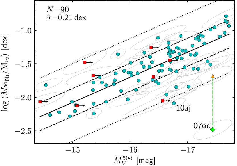
Figure 13: $\log M_{{}^{56}\mathrm{Ni}}$ against $M_{V}^{50\mathrm{d}}$. The solid line is a straight-line fit to the data (cyan circles, 90 SNe), dashed lines indicate the $\pm 1\,\hat{\sigma}$ limits around the fit, while dotted lines are the Chauvenet rejection limits. SNe with upper limits on $M_{V}^{50\mathrm{d}}$ are indicated as red squares. The green diamond corresponds to SNe 2007od, while the orange triangle is SN 2007od with a $\log M_{{}^{56}\mathrm{Ni}}$ correction of 0.8 dex. Ellipses indicate $1\,\sigma$ confidence regions, which for clarity are drawn only for SNe outside the $\pm 1\,\hat{\sigma}$ limits.

Using the model selection procedure (Appendix C), we find that the correlation between $\log M_{{}^{56}\mathrm{Ni}}$ and $M_{V}^{50\mathrm{d}}$ can be represented by the straight line

$$\log M_{{}^{56}\mathrm{Ni}}=-7.708(\pm 0.445)-0.3755(\pm 0.0271)M_{V}^{50\mathrm{d}},$$ (29)

where the parameter errors (in parentheses) are obtained performing $10^{4}$ bootstrap resamplings.

To identify outliers other than SN 2007od in the $\log M_{{}^{56}\mathrm{Ni}}$ versus $M_{V}^{50\mathrm{d}}$ distribution, we use the Chauvenet’s criterion. In Fig. 13 we see that SN 2010aj is located below the Chauvenet lower rejection limit but consistent with it within $2\,\sigma$, which means that we cannot confirm that SN as an outlier. SN 2010aj was presented in Inserra et al. (2013), which suggested that it may be affected by newly formed dust. In that work, however, the lack of further evidence did not allow confirmation of the above scenario.

In the case of SNe 2007od we consider its $\log M_{{}^{56}\mathrm{Ni}}$ values as lower limits. Indeed, based on the $M_{{}^{56}\mathrm{Ni}}$ values reported by Inserra et al. (2011), the inclusion of the IR light excess to the luminosity of SN 2007od increases its $\log M_{{}^{56}\mathrm{Ni}}$ in $\sim$0.8 dex. Applying this correction, SN 2007od moves in Fig. 13 from $-6.3$ to $-2.5\,\hat{\sigma}$ below the fit, becoming consistent with the $\log M_{{}^{56}\mathrm{Ni}}$ versus $M_{V}^{50\mathrm{d}}$ distribution.

4.3.3 Sample completeness

The SNe in our set were selected from the literature by having at least three photometric points in the radioactive tail, so our sample is potentially affected by the selection bias. In order to correct for the latter bias and construct an SN sample as complete as possible, we use as reference the volume-limited SN sample of Shivvers et al. (2017). Most of the SNe II in that sample have completeness $\gtrsim$95 per cent at the cut-off distance of 38 Mpc ($\mu=32.9$ mag), while sub-luminous and highly reddened SNe have completeness $\gtrsim$70 per cent (see Fig. 4 of Li et al. 2011). Therefore, we assume that the set of normal SNe II at $\mu<32.9$ in the Shivvers et al. (2017) sample is roughly complete.

From the Shivvers et al. (2017) sample we select the 28 normal SNe II with $\mu<32.9$ mag (hereafter the RC set), where we use $\mu$ values computed with the procedure described in Section 3.6.1 (reported in Column 8 of Table 16). We recalibrate their absolute $R$ magnitudes ($M_{R}$) at maximum ($M_{R}^{\max}$, listed in Li et al. 2011) using our $\mu$ values, and correcting for $E_{{B\!-\!V}}^{\mathrm{h}}$ (estimated with the procedure described in Section 3.6.2, and reported in Column 6 of Table 17). We also replace the Schlegel et al. (1998) $E_{{B\!-\!V}}^{\mathrm{G}}$ values used in Li et al. (2011) by the new ones provided by Schlafly & Finkbeiner (2011). Table 21 lists the $M_{R}^{\max}$ estimates for the RC sample.

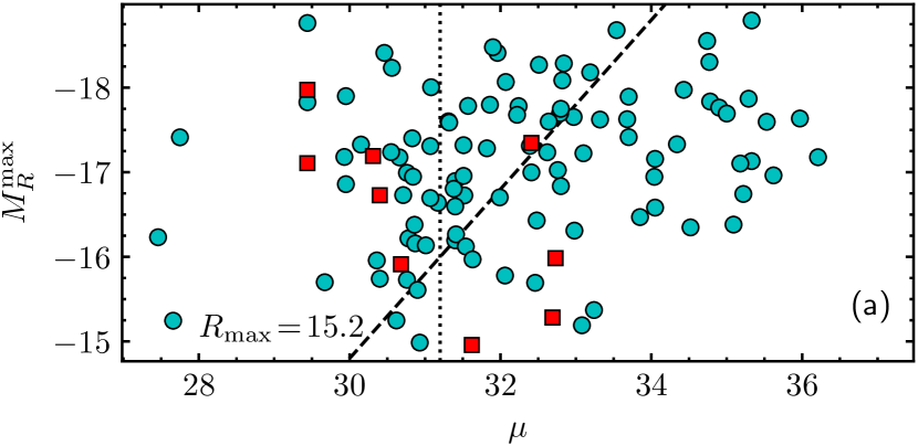
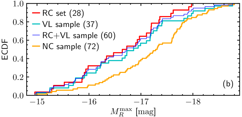
Figure 14: Panel (a): $M_{R}^{\max}$ against $\mu$ for the SNe in our sample, where red squares are the SNe in common with the RC set. The dashed line corresponds to ${R_{\max}}=15.2$ mag, while the dotted line (${\mu=31.2}$) is the limit for our VL sample. Panel (b): ECDF for the $M_{R}^{\max}$ values in the RC (red line), VL (cyan line), and RC+VL (thin blue line) samples, and for the $M_{R}^{\max}$ values of the SNe in our sample with ${\mu>31.2}$ (orange line).

Among the 109 SNe in our sample, nine have $M_{R}^{\max}$ estimates provided in the RC set, so we adopt those values for consistency. Out of the remaining 100 SNe:

• Forty-seven SNe have $R$- or $r$-band light curves during the maximum light, where $r$ magnitudes are converted into $R$ ones using ${r\!-\!R=0.12}$ (see Appendix H). We measure $M_{R}^{\max}$ performing an ALR fit to the maximum photometry or adopting the brightest $M_{R}$ value ($M_{R}^{\mathrm{br}}$) as $M_{R}^{\max}$. The average of the rise time ($t_{R}^{\mathrm{rise}}$) for the latter SNe is of $15\pm 6$ d ($1\,\hat{\sigma}$ error), while the mean $V\!-\!R$ and $R\!-\!I$ colours at time $t_{R}^{\mathrm{rise}}$ are of $0.15\pm 0.08$ and $0.04\pm 0.07$ mag, respectively.

• Thirty SNe have $R/r$ light curves where the maximum light cannot be determined; six SNe have $V\!I$ photometry, which we convert into $R$ magnitudes using ${V\!-\!R=0.05+0.59({V\!-\!I})}$ (see Appendix H); and eight SNe (one SN) only have $V$-band ($I$-band) photometry, which we convert into $R$ magnitudes using $V\!-\!R=0.15$ ($R\!-\!I=0.04$). For each of these 45 SNe we fit a straight line to the light curve, compute $M_{R}$ at $t_{R}^{\mathrm{rise}}$ ($M_{R}(t_{R}^{\mathrm{rise}})$), and adopt the minimum between $M_{R}^{\mathrm{br}}$ and $M_{R}(t_{R}^{\mathrm{rise}})$ as $M_{R}^{\max}$.

• Eight SNe have photometry starting at ${\Delta t>80}$ d. Two of them (SNe 1997D and 2004eg) are sub-luminous SNe II, which tend to have flat light curves during the photospheric phase (e.g. Spiro et al., 2014), so we adopt $M_{R}^{\mathrm{br}}$ as $M_{R}^{\max}$. For the remaining six SNe we estimate $M_{R}^{\mathrm{max}}$ using their $\log M_{{}^{56}\mathrm{Ni}}$ values and $M_{R}^{\max}=-20.01-1.86\log M_{{}^{56}\mathrm{Ni}}$, obtained from the 47 SNe with well-defined maximum light.

The $M_{R}^{\max}$ values for the SNe in our sample are reported in Table 21 and plotted in Fig. 14(a) against $\mu$. The mean apparent $R$-band magnitude at maximum ($R_{\max}$, corrected for reddening) is of 15.2 mag, which is indicated as a dashed line. As we move to greater $R_{\max}$ values (right-hand side of the dashed line) we see a decrement in the number of SNe, which is due to (1) bright SNe (in apparent magnitude) are more likely to be selected for photometric monitoring in the radioactive tail than faint ones; and (2) faint SNe have in general less photometric points in the radioactive tail than bright ones, so they are more likely not to meet our selection criterion of having at least three photometric points. In order to minimize the effect of the selection bias, we construct a volume-limited (VL) sample with the 37 SNe at $\mu\leq 31.2$ such that the selection bias could be relevant only in the small region between $R_{\max}>15.2$ and $\mu\leq 31.2$.

Fig. 14(b) shows the empirical cumulative distribution function (ECDF) for the $M_{R}^{\max}$ values in the VL (cyan line) and the RC (red line) samples. To test whether both $M_{R}^{\max}$ samples are drawn from a common unspecified distribution (the null hypothesis), we use the two-sample Anderson-Darling (AD) test (e.g. Scholz & Stephens, 1987). We obtain a standardized test statistic ($T_{\mathrm{AD}}$) of $-0.65$ with a $p$-value of 0.74, meaning that the null hypothesis cannot be rejected at a significance level $>$74 per cent. Since the $M_{R}^{\max}$ values of the RC and the VL samples are likely drawn from the same $M_{R}^{\max}$ distribution, we can assume that the completeness of both samples is quite similar, so we combine them into a single data set (RC+VL). The $M_{R}^{\max}$ ECDF of the RC+VL sample (blue thin line) has a minimum, maximum, mean and $\hat{\sigma}$ of $-18.8$, $-15.0$, $-16.7$, and $0.9$ mag, respectively.

Fig. 14(b) also shows the ECDF for the $M_{R}^{\max}$ values of the 72 SNe at $\mu>31.2$ (orange line), which we refer as the non-complete (NC) sample. Using the two-sample AD test to test the null hypothesis for the $M_{R}^{\max}$ values of the RC+VL and the NC samples, we obtain a $T_{\mathrm{AD}}$ of $5.66$ and a $p$-value of 0.002. Thus, the null hypothesis can be rejected at a significance level of 0.2 per cent, which is expected since the NC sample is affected by the selection bias.

In order to roughly quantify the number and magnitudes of the SNe missing from the NC sample, and therefore from our full sample, we proceed as follows. First, we divide the $M_{R}^{\max}$ distribution into four bins of width 1 mag (Column 1 of Table 4), and register the number of SNe within each bin for the NC and the RC+VL samples (Columns 2 and 3, respectively). Then, since bright SNe are less affected by the selection bias, we scale the number of SNe in the RC+VL sample by a factor of 15/8 (Column 4) in order to match the number of SNe with $M_{R}^{\max}<-17.8$ to that of the NC sample. In other words, the numbers in Column 4 are the SNe we would expect for a roughly complete sample with 15 SNe at $M_{R}^{\max}<-17.8$. The number of expected SNe minus the observed ones (i.e. the NC sample) is listed in Column 5. Thus, to correct our full SN sample for selection bias, we have to include 3, 23, and 15 SNe of magnitude ${-17.8\leq M_{R}^{\max}<-16.8}$, ${-16.8\leq M_{R}^{\max}<-15.8}$, and ${M_{R}^{\max}\geq-15.8}$, respectively. The latter SNe can be randomly selected from the VL or the RC+VL sample within the corresponding $M_{R}^{\max}$ bins.

Table 4: Histogram for $M_{R}^{\max}$.

$M_{R}^{\max}$ range	NC	RC+VL	Expected	Missing
$-17.8,\,-18.8$	15	8	15	0
$-16.8,\,-17.8$	36	21	39	3
$-15.8,\,-16.8$	15	20	38	23
$-14.8,\,-15.8$	6	11	21	15
Notes: $\mathrm{Expected}=15/8\mathrm{(RC+VL)}$. $\mathrm{Missing}=\mathrm{Expected}\!-\!\mathrm{NC}$.

4.3.4 Mean ⁵⁶Ni mass

Fig. 15 shows the ECDFs for the $M_{{}^{56}\mathrm{Ni}}$ values in the VL (cyan line) and the full (blue line) samples. The ECDF of the VL sample has a $\langle M_{{}^{56}\mathrm{Ni}}\rangle$ and $\hat{\sigma}$ of 0.037 and 0.032 $\mathrm{M}_{\sun}$, respectively, while the random error (ran) on the mean ($\hat{\sigma}/\sqrt{N}$) is of $0.005\,\mathrm{M}_{\sun}$. On the other hand, the $M_{{}^{56}\mathrm{Ni}}$ distribution of the full sample has a minimum, maximum, mean, and $\hat{\sigma}$ of 0.005, 0.177, 0.042, and $0.033\,\mathrm{M}_{\sun}$, respectively, with $\hat{\sigma}/\sqrt{N}=0.003\,\mathrm{M}_{\sun}$. The latter mean value corresponds to $\langle M_{{}^{56}\mathrm{Ni}}\rangle$ uncorrected for selection bias ($\langle M_{{}^{56}\mathrm{Ni}}\rangle^{\mathrm{unc}}$) which, as expected, is greater than the $\langle M_{{}^{56}\mathrm{Ni}}\rangle$ estimate for the VL sample. We note that for models based on the neutrino-heating mechanism (the generally accepted one for CC SNe, e.g. Burrows & Vartanyan 2021) the upper limit for the synthesized $M_{{}^{56}\mathrm{Ni}}$ is around 0.15 and 0.23 $\mathrm{M}_{\sun}$ (e.g. Ugliano et al., 2012; Suwa et al., 2019), which is consistent with the maximum $M_{{}^{56}\mathrm{Ni}}$ of our full SN sample.

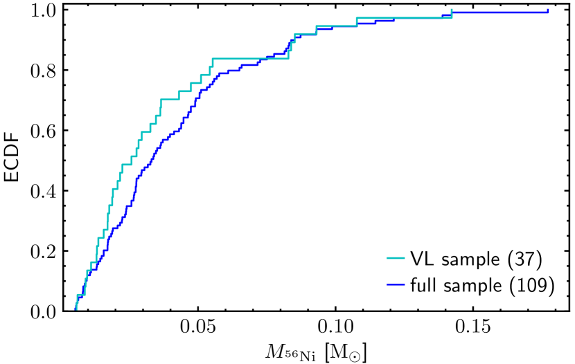
Figure 15: ECDF for the ⁵⁶Ni masses in the VL (cyan line) and the full sample (blue line).

The random error on $\langle M_{{}^{56}\mathrm{Ni}}\rangle^{\mathrm{unc}}$ is made up of the sampling error along with the uncertainties induced by errors in $\mu$ and $E_{{B\!-\!V}}^{\mathrm{h}}$. To estimate the random error in $\langle M_{{}^{56}\mathrm{Ni}}\rangle^{\mathrm{unc}}$ induced by uncertainties in $\mu$, we perform $10^{5}$ simulations varying randomly $\mu$ according to its errors (assumed normal). For each realization, we rescale the $\log M_{{}^{56}\mathrm{Ni}}$ values of the SNe in our full sample using the simulated $\mu$ values and calculate the mean ⁵⁶Ni mass. Using those $10^{5}$ simulated mean values we compute a $\hat{\sigma}$ around $\langle M_{{}^{56}\mathrm{Ni}}\rangle^{\mathrm{unc}}$ of $0.0009\,\mathrm{M}_{\sun}$, which we adopt as the error induced by uncertainties in $\mu$. We repeat the same process for $E_{{B\!-\!V}}^{\mathrm{h}}$, obtaining $0.0011\,\mathrm{M}_{\sun}$. The random error on $\langle M_{{}^{56}\mathrm{Ni}}\rangle^{\mathrm{unc}}$ is $0.0028\,\mathrm{M}_{\sun}$ greater in quadrature than the error induced by $\mu$ and $E_{{B\!-\!V}}^{\mathrm{h}}$. We adopt the latter value as the sampling error.

As mentioned in Section 4.3.3, to correct our full SN sample for selection bias we have to include 41 SNe. The mean ⁵⁶Ni mass of the selection-bias-corrected sample can be written as

$$\langle M_{{}^{56}\mathrm{Ni}}\rangle=\langle M_{{}^{56}\mathrm{Ni}}\rangle^{\mathrm{unc}}-\mathrm{sbc}.$$ (30)

Here,

$$\mathrm{sbc}=\frac{41}{109+41}(\langle M_{{}^{56}\mathrm{Ni}}\rangle^{\mathrm{unc}}-\langle M_{{}^{56}\mathrm{Ni}}\rangle_{41}^{\mathrm{unc}})$$ (31)

is the selection bias correction, where $\langle M_{{}^{56}\mathrm{Ni}}\rangle_{41}^{\mathrm{unc}}$ is the mean ⁵⁶Ni mass computed with the 41 SNe that we have to add to our full SN sample. Performing $10^{5}$ simulations, where the missing SNe (Column 5 of Table 4) are randomly selected from the VL sample within the corresponding $M_{R}^{\max}$ bins, we obtain a sbc of $0.005\pm 0.001\,\mathrm{M}_{\sun}$. Therefore, our best estimate of $\langle M_{{}^{56}\mathrm{Ni}}\rangle$ for normal SNe II is of $0.037\pm 0.003\,\mathrm{(ran)}\,\mathrm{M}_{\sun}$, with a systematic error due to the uncertainty on $\mathrm{ZP}^{\mathrm{BC}}$ and $\alpha$ of $0.004\,\mathrm{M}_{\sun}$. This result compares to the $\langle M_{{}^{56}\mathrm{Ni}}\rangle$ value of $0.037\pm 0.005\,\mathrm{(ran)}\,\mathrm{M}_{\sun}$ obtained with the VL sample.

Table 5 summarizes the error budget for $\langle M_{{}^{56}\mathrm{Ni}}\rangle$. The $\mathrm{ZP}_{I}^{\mathrm{BC}}$ error, accounting for 46 per cent of the total uncertainty, dominates the error budget. The sampling error, which is the main source of random uncertainty, accounts for 31 per cent of the total error.

Table 5: Error budget for the mean ⁵⁶Ni mass.

Error type	Error	Typical	Error in	% of total
	source	error	$\langle M_{{}^{56}\mathrm{Ni}}\rangle$	error
			($\mathrm{M}_{\sun}$)
Random	Sampling	0.0028 $\mathrm{M}_{\sun}$	0.0028	31.0
	sbc	0.0014 $\mathrm{M}_{\sun}$	0.0014	7.7
	$E_{{B\!-\!V}}^{\mathrm{h}}$	0.08 mag	0.0011	4.8
	$\mu$	0.18 mag	0.0009	3.2
	All		0.00344	46.7
Systematic	$\mathrm{ZP}^{\mathrm{BC}}$	0.10 mag	0.0034	45.6
	$\alpha$	3.9 %	0.0014	7.7
	All		0.00368	53.3
Total			0.00504	100.0

4.4 Mean iron yield

With our $\langle M_{{}^{56}\mathrm{Ni}}\rangle$ measurement along with equation (21) and ${\eta=1.07\pm 0.04}$ (see Section 3.5), we obtain a $\bar{y}_{\mathrm{Fe}}$ value of ${0.040\pm 0.005\,\mathrm{M}_{\sun}}$ for normal SNe II.

In addition, we evaluate $\bar{y}_{\mathrm{Fe}}$ for CC SNe employing recent estimations of mean ⁵⁶Ni masses for other CC SN subtypes. The mean ⁵⁶Ni mass for CC SNe, using the SN rates provided in Shivvers et al. (2017), is given by

$$f_{\mathrm{CC}}^{\mathrm{Ni}}=0.696f^{\mathrm{Ni}}_{\mathrm{II}}+0.304f^{\mathrm{Ni}}_{\mathrm{SE}}.$$ (32)

Here,

$$f_{\mathrm{II}}^{\mathrm{Ni}}=0.891f^{\mathrm{Ni}}_{\text{II-normal}}+0.067f^{\mathrm{Ni}}_{\mathrm{IIn}}+0.042f^{\mathrm{Ni}}_{\text{long-rising}}$$ (33)

and

$$f_{\mathrm{SE}}^{\mathrm{Ni}}=0.360f_{\mathrm{IIb}}^{\mathrm{Ni}}+0.356f_{\mathrm{Ib}}^{\mathrm{Ni}}+0.247f_{\mathrm{Ic}}^{\mathrm{Ni}}+0.037f_{\text{Ic-BL}}^{\mathrm{Ni}},$$ (34)

where $f^{\mathrm{Ni}}$ denotes the mean ⁵⁶Ni mass for the subscripted CC SN types and subtypes.

In equation (33) we adopt ${f^{\mathrm{Ni}}_{\text{long-rising}}=0.086\,\mathrm{M}_{\sun}}$ (Anderson, 2019) and for SNe IIn we assume ${f^{\mathrm{Ni}}_{\mathrm{IIn}}=f^{\mathrm{Ni}}_{\text{II-normal}}}$, thus obtaining ${f^{\mathrm{Ni}}_{\mathrm{II}}=0.039\,\mathrm{M}_{\sun}}$.

For SNe IIb, Ib, Ic and Ic-BL we adopt the mean $M_{{}^{56}\mathrm{Ni}}$ values from the compilation of Anderson (2019): 0.124, 0.199, 0.198, and 0.507 $\mathrm{M}_{\sun}$, respectively. The ⁵⁶Ni masses of the SE SNe compiled by Anderson (2019) were mainly computed with the Arnett (1982) rule, which overestimates the ⁵⁶Ni mass of SE SNe by $\sim$50 per cent (Dessart et al., 2015, 2016). Including this correction to the mean $M_{{}^{56}\mathrm{Ni}}$ values of SE SNe, with equation (34) we get ${f^{\mathrm{Ni}}_{\mathrm{SE}}=0.122\,\mathrm{M}_{\sun}}$. Recently, by using the radioactive tail luminosity, Afsariardchi et al. (2020) estimated mean $M_{{}^{56}\mathrm{Ni}}$ values of 0.06, 0.11, 0.20, and $0.15\,\mathrm{M}_{\sun}$ for SNe IIb, Ib, Ic, and Ic-BL, respectively. Inserting these values in equation (33) we get ${f^{\mathrm{Ni}}_{\mathrm{SE}}=0.116\,\mathrm{M}_{\sun}}$, which is similar to the previous finding. Since the SN samples of Anderson (2019) and Afsariardchi et al. (2020) are not corrected for selection bias, we adopt ${f^{\mathrm{Ni}}_{\mathrm{SE}}<0.12\,\mathrm{M}_{\sun}}$

Replacing the $f^{\mathrm{Ni}}_{\mathrm{SE}}$ and $f^{\mathrm{Ni}}_{\mathrm{II}}$ values in equation (32), we get ${f^{\mathrm{Ni}}_{\mathrm{CC}}<0.064\,\mathrm{M}_{\sun}}$, where the contribution of normal SNe II to $f^{\mathrm{Ni}}_{\mathrm{CC}}$ is $>$36 per cent. Finally, if we assume ${\eta=1.07}$ for all CC SN subtypes, then from equation (21) we obtain ${\bar{y}_{\mathrm{Fe}}<0.068\,\mathrm{M}_{\sun}}$ for CC SNe.

4.5 Steepness as ⁵⁶Ni mass indicator

From the analysis of nine normal SNe II and the long-rising SN 1987A, Elmhamdi et al. (2003b) reported a linear correlation between $\log M_{{}^{56}\mathrm{Ni}}$ and the maximum value of $dV/dt$ during the transition phase, called $V$-band steepness $S_{V}$. This correlation was also rebuilt by Singh et al. (2018), which included another 30 SNe to the sample of Elmhamdi et al. (2003b). The observed correlation is proposed to be a consequence of the ⁵⁶Ni heating during the transition phase (e.g. Pumo & Zampieri, 2011, 2013). The latter produces slower transitions of the luminosity from the end of the plateau phase to the beginning of the radioactive tail as $M_{{}^{56}\mathrm{Ni}}$ increases. Since the correlation between $\log M_{{}^{56}\mathrm{Ni}}$ and steepness has not been studied for bands other than $V$, in this work we will include the $gr\!RiI$ bands in the analysis.

In order to measure the $x$-band steepness, $S_{x}$, we represent the light-curve transition phase by the function

$$m_{x}(t)=m_{0,x}-\frac{a_{0,x}}{1+e^{(t-t_{\mathrm{PT},x})/w_{0,x}}}+p_{0,x}\frac{t-t_{\mathrm{PT},x}}{100\,\mathrm{d}}$$ (35)

(e.g. Olivares E. et al., 2010; Valenti et al., 2016). The parameters $m_{0,x}$, $a_{0,x}$, $t_{\mathrm{PT},x}$ (the middle of the transition phase), $w_{0,x}$, and $p_{0,x}$ are obtained maximizing the model log-likelihood (equation 50). Fig. 16 shows this analytical fit applied to the $V$-band photometry of SN 2014G. Using the aforementioned parametric function, the $x$-band steepness (in mag d^-1) in the SN rest frame is given by

$$S_{x}=\left(\frac{a_{0,x}}{4w_{0,x}}+\frac{p_{0,x}}{100\,\mathrm{d}}\right)/(1+z^{\mathrm{SN}}_{\mathrm{helio}}).$$ (36)

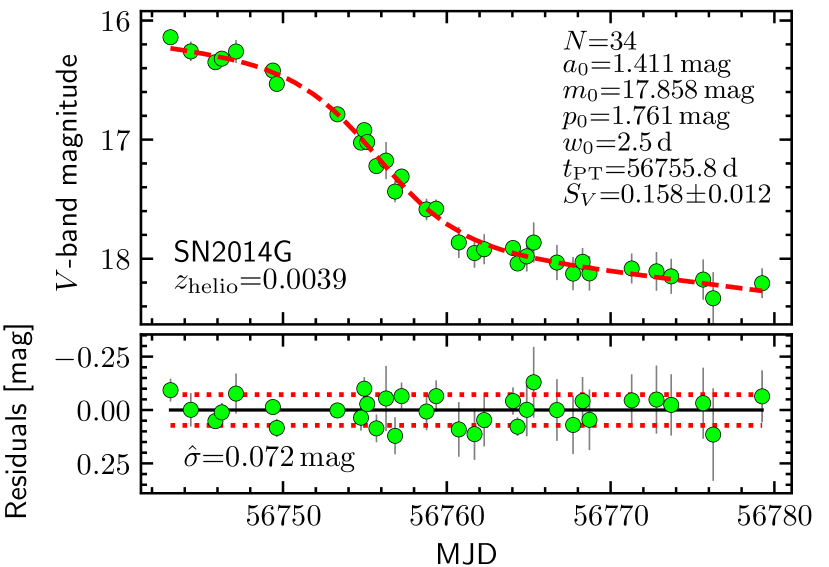
Figure 16: Top panel: $V$-band light curve of SN 2014G in the transition phase, where the dashed line corresponds to the best fit. Bottom panel: best fit residuals, where dotted lines indicate the $\pm 1\,\hat{\sigma}$ limits. Error bars are $1\,\sigma$ errors.

Columns 2–7 of Table 22 list the $gV\!r\!RiI$-band $S_{x}$ values and their bootstrap errors. As visible in the table, the $S_{x}$ estimates are in general not available for each of the $gV\!r\!RiI$ bands. In those cases we estimate $S_{x}$ indirectly from the steepnesses in bands other than $x$ (see Appendix J). These indirect $S_{x}$ values ($S_{x}^{*}$) for the $gV\!r\!RiI$ bands and their errors are in Columns 8–13 of Table 22. Table 6 lists the mean and $\hat{\sigma}$ values of the $S_{x}^{*}\!-\!S_{x}$ estimates for the $gV\!r\!RiI$ bands. The mean values are statistically consistent with zero within $1\,\hat{\sigma}/\sqrt{N}$. Therefore, for SNe without an specific $S_{x}$ value, we can use their respective $S_{x}^{*}$ as a proxy.

Table 6: Mean $S_{x}^{*}\!-\!S_{x}$ values.

$x$	$\langle S_{x}^{*}\!-\!S_{x}\rangle$	$\hat{\sigma}$	$N$	$x$	$\langle S_{x}^{*}\!-\!S_{x}\rangle$	$\hat{\sigma}$	$N$
$g$	$-0.002$	0.016	16	$V$	$-0.003$	0.024	41
$r$	$0.003$	0.029	20	$R$	$-0.002$	0.017	32
$i$	$-0.004$	0.036	22	$I$	$0.002$	0.018	31
Note. Mean and $\hat{\sigma}$ values are in mag d-1 units.

Fig. 17 shows $\log M_{{}^{56}\mathrm{Ni}}$ versus $S_{x}$ for the $gV\!r\!RiI$ bands. Through the model selection procedure (Appendix C), we find that the correlation between $\log M_{{}^{56}\mathrm{Ni}}$ and $S_{x}$ is well represented by the straight line

$$\log M_{{}^{56}\mathrm{Ni}}=c_{0,x}+c_{1,x}S_{x}$$ (37)

which, for the $V$-band, corresponds to the best fit proposed by Elmhamdi et al. (2003b). The parameters $c_{0,x}$ and $c_{1,x}$ (and their bootstrap errors) for the $gV\!r\!RiI$ bands are reported in Table 7. To evaluate the linear correlation between $\log M_{{}^{56}\mathrm{Ni}}$ and $S_{x}$, we calculate the Pearson correlation coefficient $r_{x}$, listed in Column 6 of Table 7. The probability of obtaining ${|r_{x}|\geq 0.65}$ from a random population with ${N=72}$ is $<$0.001 per cent.

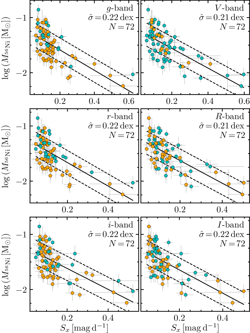
Figure 17: $\log M_{{}^{56}\mathrm{Ni}}$ against $S_{x}$ for $gV\!r\!RiI$ bands. Cyan circles are SNe with $S_{x}$ measured from their $x$-band light curves, while orange circles are SNe with $S_{x}$ estimated from the steepnesses in other bands. Solid lines are straight-line fits to the data, dashed lines are $\pm 1\,\hat{\sigma}$ limits around the fits, and error bars are $1\,\sigma$ errors.

Table 7: $\log M_{{}^{56}\mathrm{Ni}}$ versus $S_{x}$ calibrations.

$x$	$c_{0,x}$	$c_{1,x}$	$\hat{\sigma}$	$N$	$r_{x}$
	(dex)	(dex)	(dex)
$g$	$-1.219\pm 0.049$	$-1.844\pm 0.256$	0.217	72	$-0.67$
$V$	$-1.201\pm 0.043$	$-1.789\pm 0.183$	0.210	72	$-0.69$
$r$	$-1.238\pm 0.047$	$-2.130\pm 0.292$	0.219	72	$-0.66$
$R$	$-1.217\pm 0.042$	$-2.053\pm 0.217$	0.210	72	$-0.69$
$i$	$-1.237\pm 0.044$	$-1.901\pm 0.231$	0.221	72	$-0.65$
$I$	$-1.223\pm 0.045$	$-2.106\pm 0.253$	0.219	72	$-0.66$
Notes. $\log M_{{}^{56}\mathrm{Ni}}=c_{0,x}+c_{1,x}S_{x}$. $M_{{}^{56}\mathrm{Ni}}$ and $S_{x}$ are in $\mathrm{M}_{\sun}$ and mag d-1 units, respectively.

The observed $\hat{\sigma}$ of 0.21–0.22 dex for the $gV\!r\!RiI$ bands indicates that there is no preferred band for the $\log M_{{}^{56}\mathrm{Ni}}$ versus $S_{x}$ correlation. Since the $\hat{\sigma}$ values are $\sim$0.17 dex greater in quadrature than the typical random error (0.13 dex), the observed dispersion is mainly intrinsic. The latter was also pointed out by Pumo & Zampieri (2013). Indeed, the shape of light curves in the transition phase not only depends on $M_{{}^{56}\mathrm{Ni}}$ but also, among others, on the H mass retained before the explosion and the ⁵⁶Ni mixing (e.g. Young, 2004; Bersten et al., 2011; Kozyreva et al., 2019).

Fig. 18 shows the residuals of the $\log M_{{}^{56}\mathrm{Ni}}$ versus $S_{V}$ correlation (i.e. upper-right panel of Fig. 17) plotted against $M_{V}^{50\mathrm{d}}$, where we detect a linear dependence of the residuals on $M_{V}^{50\mathrm{d}}$. Therefore the Elmhamdi et al. (2003b) relation over and underestimates the $\log M_{{}^{56}\mathrm{Ni}}$ of sub-luminous and moderately-luminous SNe II, respectively, by up to $\sim$0.3 dex. This fact, along with the low statistical precision of the Elmhamdi et al. (2003b) relation to measure $M_{{}^{56}\mathrm{Ni}}$ (around 50 per cent), makes the latter method poorly suited for ⁵⁶Ni mass measurements.

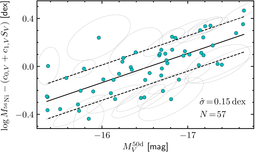
Figure 18: Residuals of the $\log M_{{}^{56}\mathrm{Ni}}$ versus $S_{V}$ correlation, as a function of $M_{V}^{50\mathrm{d}}$. The solid and dashed lines have the same meaning than in Fig 17. Ellipses are 1 $\sigma$ confidence regions, which for clarity are drawn only for SNe outside the dashed lines.

4.6 Nickel-magnitude-steepness relation

Our previous finding suggests a correlation of $\log M_{{}^{56}\mathrm{Ni}}$ as a function not only of $S_{x}$ but also of the $x$-band absolute magnitude at ${\Delta t=50}$ d ($M_{x}^{50\mathrm{d}}$). The $M_{x}^{50\mathrm{d}}$ values for $gr\!RiI$ are listed in Table 24. If $M_{x}^{50\mathrm{d}}$ is not available for a given band, then we estimate it using photometry in other bands and magnitude transformation formulae (see Appendix H).

Using the model selection procedure (Appendix C), we find that the correlation of $\log M_{{}^{56}\mathrm{Ni}}$ as a function of $S_{x}$ and $M_{x}^{50\mathrm{d}}$ can be represented by

$$\log M_{{}^{56}\mathrm{Ni}}=a_{x}+b_{x}M_{x}^{50\mathrm{d}}+c_{x}\log S_{x},$$ (38)

where $\log S_{x}$ is given by equation (62). Fig. 19 shows the nickel-magnitude-steepness (NMS) relation for the $gV\!r\!RiI$ bands, while Table 8 lists the parameters (and their bootstrap errors) of equation (38) along with the ranges of $M_{x}^{50\mathrm{d}}$ and $\log S_{x}$ where the relation is valid. To evaluate the linear correlation of $\log M_{{}^{56}\mathrm{Ni}}$ on $M_{x}^{50\mathrm{d}}$ and $\log S_{x}$, we calculate the multiple correlation coefficient ($R_{x}^{\mathrm{mc}}$, reported in Column 10 of Table 8). The probability of obtaining $R_{x}^{\mathrm{mc}}\geq 0.89$ from a random population is $<$0.001 per cent.

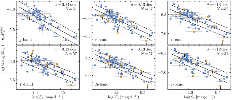
Figure 19: NMS relations for the $gV\!r\!RiI$ bands. Solid lines are the best fits to the data (circles), while dashed lines indicate the $\pm 1\,\hat{\sigma}$ limits around the fits. Orange squares correspond to SNe with lower/upper limits on $M_{x}^{50\mathrm{d}}$. Error bars are $1\,\sigma$ errors.

Table 8: NMS relation parameters.

$x$	$a_{x}$	$b_{x}$	$c_{x}$	$\hat{\sigma}$	$\sigma_{0,x}$	$N$	$M_{x}^{50\mathrm{d}}$ range	$\log S_{x}$ range	$R_{x}^{\mathrm{mc}}$
	(dex)	(dex mag-1)		(dex)	(dex)		(mag)	(dex)
$g$	$-5.894\pm 0.461$	$-0.2311\pm 0.0306$	$-0.750\pm 0.097$	$0.136$	$0.112$	51	$-14.9,\,-17.4$	$-1.26,\,-0.21$	0.89
$V$	$-6.612\pm 0.409$	$-0.2778\pm 0.0266$	$-0.608\pm 0.083$	$0.132$	$0.106$	57	$-15.4,\,-17.7$	$-1.22,\,-0.23$	0.89
$r$	$-6.683\pm 0.459$	$-0.2710\pm 0.0294$	$-0.669\pm 0.087$	$0.132$	$0.107$	57	$-15.6,\,-18.1$	$-1.39,\,-0.29$	0.90
$R$	$-6.315\pm 0.449$	$-0.2487\pm 0.0287$	$-0.673\pm 0.082$	$0.128$	$0.094$	57	$-15.7,\,-18.2$	$-1.39,\,-0.30$	0.90
$i$	$-7.154\pm 0.442$	$-0.3066\pm 0.0281$	$-0.590\pm 0.079$	$0.127$	$0.098$	52	$-15.4,\,-17.7$	$-1.33,\,-0.28$	0.90
$I$	$-7.324\pm 0.430$	$-0.3083\pm 0.0267$	$-0.608\pm 0.080$	$0.124$	$0.098$	52	$-15.7,\,-18.1$	$-1.32,\,-0.30$	0.91
Notes. $\log M_{{}^{56}\mathrm{Ni}}=a_{x}+b_{x}M_{x}^{50\mathrm{d}}+c_{x}\log S_{x}$. $M_{{}^{56}\mathrm{Ni}}$, $M_{x}^{50\mathrm{d}}$, and $S_{x}$ are in units of $\mathrm{M}_{\sun}$, mag, and mag d-1, respectively.

The NMS relation allows to measure $\log M_{{}^{56}\mathrm{Ni}}$ with a statistical precision of 0.12–0.14 dex ($M_{{}^{56}\mathrm{Ni}}$ error of $\sim$30 per cent). The observed random error is about 0.08 dex, so the intrinsic random error on the NMS relation ($\sigma_{0,x}$, listed in Column 6 of Table 8) is around 0.10 dex. Since $\sim$80 per cent of the SNe used to calibrate equation (38) have $\log M_{{}^{56}\mathrm{Ni}}$ computed with $I$- or $i$-band photometry, we adopt a systematic uncertainty due to the $\mathrm{ZP}^{\mathrm{BC}}$ errors of 0.044 dex (the average between the errors on $\mathrm{ZP}_{I}^{\mathrm{BC}}$ and $\mathrm{ZP}_{i}^{\mathrm{BC}}$ in dex scale). The total systematic error ($\sigma_{\mathrm{sys}}$), including the uncertainty due to $\alpha$, is of 0.047 dex, while the total error on $\log M_{{}^{56}\mathrm{Ni}}$ provided by the NMS relation is given by

$$\sigma_{\log M_{{}^{56}\mathrm{Ni}}}=\sqrt{(b_{x}\sigma_{M_{x}^{50\mathrm{d}}})^{2}+(c_{x}\sigma_{\log Sx})^{2}+\sigma_{0,x}^{2}+\sigma_{\mathrm{sys}}^{2}}.$$ (39)

Since $|b_{x}|<0.4$, the $\log M_{{}^{56}\mathrm{Ni}}$ values estimated with the NMS relation are less dependent on $E_{{B\!-\!V}}^{\mathrm{h}}$ and $\mu$ than those computed with the radioactive tail photometry and the BC technique (Appendix D).

As a first application of the NMS relation, we compute $\log M_{{}^{56}\mathrm{Ni}}$ estimates ($\log M_{{}^{56}\mathrm{Ni}}^{\mathrm{NMS}}$) for a sample of normal SNe II observed by the Zwicky Transient Facility (ZTF; Bellm et al. 2019; Graham et al. 2019). Specifically, we employ SNe from the ZTF bright transient survey (BTS; Fremling et al., 2020; Perley et al., 2020), which consists on SNe brighter than 19 mag. From this magnitude-limited survey, we select SNe spectroscopically classified as SNe II, discarding those (1) classified as Type IIb or IIn, (2) with long-rising light curves, (3) with less than three $r_{\mathrm{ZTF}}$ photometric points in the radioactive tail, (4) with $t_{0}$ errors greater than 10 d, and (5) with absolute magnitudes and steepnesses outside the range where the NMS relation is valid. The selected ZTF BTS (SZB) sample of 28 normal SNe II and their main properties are summarized in Table 25, while Fig. 20 shows their $r_{\mathrm{ZTF}}$ light curves. Out of the SNe in the SZB set, 24 have $M_{R}^{\max}<-17$ mag, so the sample consists mainly of moderately-luminous SNe II.

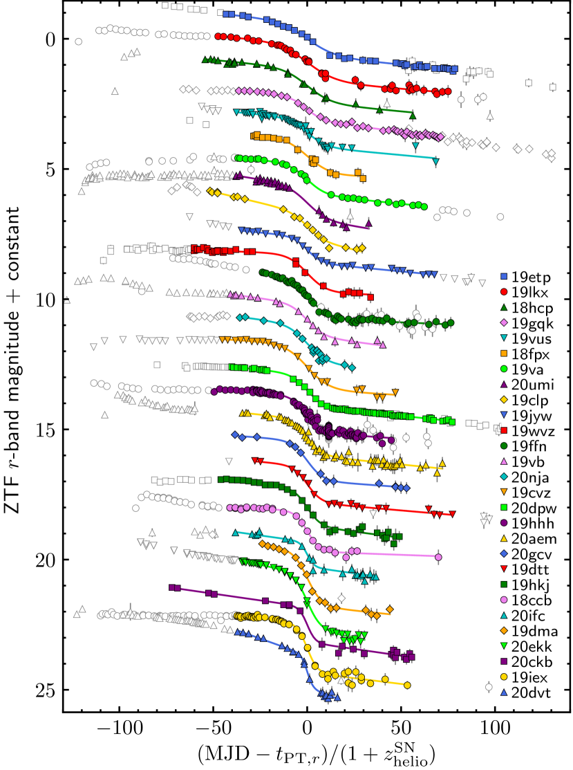
Figure 20: $r_{\mathrm{ZTF}}$ light curves of the 28 normal SNe II in the SZB sample. Data used to measure the steepness are shown with colour-filled symbols, while solid lines are analytical fits.

Given that ${r_{\mathrm{ZTF}}\!-\!R=0.14}$ mag from the photospheric to the radioactive tail phase (see Appendix H), for the $r_{\mathrm{ZTF}}$ band we adopt the $R$-band NMS relation, but with ${a_{r_{\mathrm{ZTF}}}=a_{R}-0.14b_{R}}$ equal to $-6.281$ dex. Since we cannot measure $E_{{B\!-\!V}}^{\mathrm{h}}$ for the SZB sample with the available data, we assume $E_{{B\!-\!V}}^{\mathrm{h}}=0.16\pm 0.15$ mag (the average of the $E_{{B\!-\!V}}^{\mathrm{h}}$ distribution shown in Fig. 6). Column 9 of Table 25 lists the inferred $\log M_{{}^{56}\mathrm{Ni}}^{\mathrm{NMS}}$ values. For comparison, we also compute $\log M_{{}^{56}\mathrm{Ni}}$ with the radioactive tail luminosity ($\log M_{{}^{56}\mathrm{Ni}}^{\mathrm{tail}}$, Column 10 of Table 25), using a constant $\mathrm{BC}_{r_{\mathrm{ZTF}}}=\mathrm{BC}_{R}-0.14$ equivalent to $11.93\pm 0.14$ mag.

The mean offset between the $\log M_{{}^{56}\mathrm{Ni}}^{\mathrm{tail}}$ and $\log M_{{}^{56}\mathrm{Ni}}^{\mathrm{NMS}}$ values is of 0.038 dex with a $\hat{\sigma}$ of 0.110 dex. The $\hat{\sigma}$ value is similar to that expected for the NMS relation (0.13 dex), while the offset is consistent with zero within $1.9\,\hat{\sigma}/\sqrt{N}$. As stated in Section 4.2.2, the use of the constant $\mathrm{BC}_{R}$ reported in Table 2 (${\mathrm{BC}_{R}=12.07}$) overestimates the radioactive tail luminosities (and therefore the $\log M_{{}^{56}\mathrm{Ni}}^{\mathrm{tail}}$ values) of moderately-luminous SNe II. To roughly estimate a more appropriate constant $\mathrm{BC}_{R}$ for the SZB sample, we use the $\mathrm{ZP}_{R}^{\mathrm{SN}}$ values of the nine SNe in the BC calibration set with $M_{R}^{\max}<-17$ mag, obtaining a $\mathrm{BC}_{R}$ of $12.13$ mag. Increasing $\mathrm{BC}_{r_{\mathrm{ZTF}}}$ by 0.06 mag decreases the offset from 0.046 to 0.014 dex, being consistent with zero within $0.7\,\hat{\sigma}/\sqrt{N}$. In addition, the offset decreases from $1.9\,\hat{\sigma}/\sqrt{N}$ to zero if we adopt $E_{{B\!-\!V}}^{\mathrm{h}}=0.05$ mag. Therefore, part of the offset could be due to an overestimation of the adopted $E_{{B\!-\!V}}^{\mathrm{h}}$. The results we obtain with the SZB sample provides further evidence supporting the usefulness of the NMS relation for $\log M_{{}^{56}\mathrm{Ni}}$ measurements.

5 Discussion

5.1 Comparison with other works

Table 2 summarizes the BC values for SNe II in the radioactive tail reported by Hamuy (2001), Bersten & Hamuy (2009), Maguire et al. (2010), and Pejcha & Prieto (2015a). From each value we subtract the zero-point used to define the apparent bolometric magnitude scale ($-10.89$ mag for Hamuy 2001 and Maguire et al. 2010, $-11.64$ mag for Bersten & Hamuy 2009, and $-11.48$ mag for Pejcha & Prieto 2015a). Since previous works reported constant BC values, for the comparison we use our estimates assuming a constant BC, which are also listed in the table. The BC values reported in the literature are consistent with our estimations within $\pm 1.1\,\sigma$. Except for Pejcha & Prieto (2015a), which did not report BC errors, the uncertainties provided in previous works are lower than those reported here. The latter is due to the few SNe used in previous studies to compute BCs. Indeed, they used only SN 1999em and the long-rising SN 1987A to compute BCs. It is interesting to note the good agreement between our constant BC values for $r\!RiI$ bands and those of Pejcha & Prieto (2015a) within $\pm 0.04$ mag.

Table 9: Constant BC values for the radioactive tail.

$\mathrm{BC}_{x}$ (mag)	$x$	$N$	Reference
$11.15\pm 0.06$	$V$	2a	Hamuy (2001)
$10.94\pm 0.05$	$V$	1a	Bersten & Hamuy (2009)
$11.22\pm 0.06$	$V$	2a	Maguire et al. (2010)
$11.27$	$V$	26b	Pejcha & Prieto (2015a)
$11.15\pm 0.18$	$V$	15	This work
$11.90$	$r$	26b	Pejcha & Prieto (2015a)
$11.89\pm 0.16$	$r$	15	This work
$12.07$	$R$	26b	Pejcha & Prieto (2015a)
$12.07\pm 0.14$	$R$	15	This work
$11.95$	$i$	26b	Pejcha & Prieto (2015a)
$11.91\pm 0.12$	$i$	15	This work
$12.41$	$I$	26b	Pejcha & Prieto (2015a)
$12.44\pm 0.11$	$I$	15	This work
aIt includes the long-rising SN 1987A.
bOnly six SNe with optical and near-IR photometry in the radioactive tail.

Table 10 collects the mean and $\hat{\sigma}$ values of the normal SN II $M_{{}^{56}\mathrm{Ni}}$ distributions presented in Blanc & Greggio (2008) and Müller et al. (2017). Despite the Blanc & Greggio (2008) sample includes the long-rising SN 1987A, we find that removing that SN only marginally modifies the reported mean and $\hat{\sigma}$ value. In addition, we include the mean ⁵⁶Ni mass computed with the 107 normal SNe II in the sample of Anderson (2019). Since previous estimates are not corrected for selection bias, for the comparison we use our $\langle M_{{}^{56}\mathrm{Ni}}\rangle^{\mathrm{unc}}$ value. The latter value and those from the aforementioned samples are consistent within $1.6\,\hat{\sigma}/\sqrt{N}$. It is worth mentioning that the collected $\langle M_{{}^{56}\mathrm{Ni}}\rangle^{\mathrm{unc}}$ values are not independent since they were computed with SN samples having objects in common. The number of SNe in common between a given set and our full sample is indicated in Column 5. In particular, the similarity between our result and that obtained from the Anderson (2019) sample is because both analyses have 70 per cent of SNe in common.

Table 10: Mean ⁵⁶Ni mass values for normal SNe II.

$\langle M_{{}^{56}\mathrm{Ni}}\rangle^{\mathrm{unc}\dagger}$	$\hat{\sigma}$	$N$	$\hat{\sigma}/\sqrt{N}$	${N_{c}}^{*}$	Reference‡
($\mathrm{M}_{\sun}$)	($\mathrm{M}_{\sun}$)		($\mathrm{M}_{\sun}$)
$0.066$	$0.082$	28	0.015	17	B08
$0.046$	$0.048$	38	0.008	33	M17
$0.042$	$0.044$	107	0.004	75	A19
$0.042$	$0.033$	109	0.003	–	This work
${}^{\dagger}\langle M_{{}^{56}\mathrm{Ni}}\rangle$ uncorrected for selection bias.
∗Number of SNe in common with our full sample (109 SNe).
‡B08: Blanc & Greggio (2008); M17: Müller et al. (2017); A19: Anderson (2019), selecting only normal SNe II.

We also compare the $\log M_{{}^{56}\mathrm{Ni}}$ values of the SNe in common between our SN set and the samples analysed in Müller et al. (2017), Valenti et al. (2016), and Sharon & Kushnir (2020). Müller et al. (2017) employed the methodology of Pejcha & Prieto (2015a), which computes $\log M_{{}^{56}\mathrm{Ni}}$ using the luminosity at ${\Delta t=200}$ d and equation (3) of Hamuy (2003). Valenti et al. (2016) used

$${M_{{}^{56}\mathrm{Ni}}/\mathrm{M}_{\sun}=0.075L_{\mathrm{SN}}^{\mathrm{opt}}(\Delta t)/L_{\mathrm{87A}}^{\mathrm{opt}}}(\Delta t),$$ (40)

being $L_{\mathrm{SN}}^{\mathrm{opt}}(\Delta t)$ and $L_{\mathrm{87A}}^{\mathrm{opt}}(\Delta t)$ the optical quasi-bolometric luminosity in the radioactive tail of a specific SN and of the long-rising SN 1987A, respectively. Sharon & Kushnir (2020) used the radioactive tail luminosity and the set of equations presented in Wygoda et al. (2019) to derive $\log M_{{}^{56}\mathrm{Ni}}$. For each sample we compute the differences between its $\log M_{{}^{56}\mathrm{Ni}}$ measurements, and calculate the mean offset ($\Delta$) and its $\hat{\sigma}$. Then, to track the main source of the observed dispersion, we repeat the previous process, but recomputing our $\log M_{{}^{56}\mathrm{Ni}}$ values without correcting for the $\gamma$-ray leakage (except for Sharon & Kushnir 2020, which included this correction) and using the $\mu$ and $E_{{B\!-\!V}}^{\mathrm{h}}$ values of the comparison work. The $\Delta$ and $\hat{\sigma}$ values are listed in Table 11.

Table 11: Mean $\log{M_{{}^{56}\mathrm{Ni}}}$ differences between different works.

$\log{M_{{}^{56}\mathrm{Ni}}}$ differences†	$N$	$\Delta$ (dex)	$\hat{\sigma}$ (dex)
M17$-$here	33	$-0.01$	$0.29$
M17$-$here(a)	33	$\phantom{-}0.01$	$0.28$
M17$-$here(a,b)	33	$\phantom{-}0.07$	$0.13$
M17$-$here(a,b,c)	33	$\phantom{-}0.05$	$0.08$
V16$-$here	33	$-0.15$	$0.30$
V16$-$here(a,b,c)	33	$-0.05$	$0.14$
S20$-$here	7	$-0.09$	$0.15$
S20$-$here(b,c)	7	$\phantom{-}0.02$	$0.05$
†M17: Müller et al. (2017); S20: Sharon & Kushnir (2020); V16: Valenti et al. (2016); here: this work, uncorrected for $\gamma$-ray leakage (a), and using the distance moduli (b) and colour excesses (c) of the comparison work.

From the comparison with the Müller et al. (2017) sample we obtain ${\hat{\sigma}=0.29}$ dex. This value decreases to 0.28 dex when we do not correct for $\gamma$-ray leakage, to 0.13 dex when we use the distance moduli of Müller et al. (2017), and to 0.08 dex if we also use their colour excesses. This indicates that differences between our $\log M_{{}^{56}\mathrm{Ni}}$ estimates and those of Müller et al. (2017) are mainly due to differences in the adopted distance moduli and colour excesses. Therefore, the $\hat{\sigma}$ value of 0.08 dex represents the typical $\log M_{{}^{56}\mathrm{Ni}}$ error for single SNe due to differences in the methodology used to compute $\log M_{{}^{56}\mathrm{Ni}}$. For the other two comparison samples we arrive at similar results.

The $\Delta$ value from the comparison with the sample of Müller et al. (2017) is equivalent to $3.5\,\hat{\sigma}/\sqrt{N}$, which indicates the presence of a systematic offset. We note that, of the 0.05 dex offset, 0.03 dex is due to the numerical coefficients of the equation used in Pejcha & Prieto (2015a) to compute $\log M_{{}^{56}\mathrm{Ni}}$. The remaining 0.02 dex is statistically consistent with zero within 1.4 $\hat{\sigma}/\sqrt{N}$. The $\Delta$ values from the comparison with the samples of Valenti et al. (2016) and Sharon & Kushnir (2020) are statistically consistent with zero within 2.0 and $1.0\,\hat{\sigma}/\sqrt{N}$, respectively.

5.2 Systematics

The models we use in this work (SN II spectra and nucleosynthesis yields) were generated by adopting many approximations and assumptions that help to characterize the underlying complex physical processes of SN explosions. Therefore, our $\mathrm{ZP}_{x}^{\mathrm{BC}}$, $\log M_{{}^{56}\mathrm{Ni}}$, $\langle M_{{}^{56}\mathrm{Ni}}\rangle$, and $\bar{y}_{\mathrm{Fe}}$ values are potentially affected by systematics on the spectral models, while $\bar{y}_{\mathrm{Fe}}$ is also affected by systematics on nucleosynthesis yield models. An analysis and quantification of those systematics is beyond the scope of this study.

5.2.1 Local Hubble-Lemaître constant

The distance moduli of 92 SNe in our sample were estimated as the weighted average of $\mu_{\mathrm{TF}}$, $\mu_{\mathrm{HLL}}$, and $\mu_{\mathrm{SVF}}$ (see Section 3.6.1). The latter are anchored to Cepheid-calibrated $H_{0}$ values of around 75 km s^-1 Mpc^-1. If we adopt a TRGB-calibrated $H_{0}$ value between 69.6 and 72.4 km s^-1 Mpc^-1 (e.g. Freedman et al., 2020; Yuan et al., 2019), then the $\mu$ values of our SN sample increase by about 0.08–0.16 mag. In this case, we obtain $\langle M_{{}^{56}\mathrm{Ni}}\rangle$ values around 0.040–0.044 $\mathrm{M}_{\sun}$. If we assume that the true local $H_{0}$ value lies between 71 and 75 km s^-1 Mpc^-1 with a uniform probability, then the systematic offset in $\langle M_{{}^{56}\mathrm{Ni}}\rangle$ induced by the $H_{0}$ uncertainty ranges between 0.0 and 0.005 $\mathrm{M}_{\sun}$, with a mean of ${0.002\pm 0.001\,\mathrm{M}_{\sun}}$. This systematic error is lower than that induced by the $\mathrm{ZP}^{\mathrm{BC}}$ error ($0.003\,\mathrm{M}_{\sun}$). Therefore the $H_{0}$ uncertainty is not so relevant for our current analysis.

5.2.2 Early dust formation

To compute $\log M_{{}^{56}\mathrm{Ni}}$ we assumed that the extinction along the SN line of sight is constant for ${\Delta t\leq 320}$ d. However, normal SNe II are dust factories, where the onset of the dust formation is different for each SN. In some cases, the dust formation begins as early as ${\Delta t\sim 100}\text{\textendash}200$ d (e.g. SN 2007od, Andrews et al. 2010, Inserra et al. 2011; SN 2011ja, Andrews et al. 2016; SN 2017eaw, Rho et al. 2018, Tinyanont et al. 2019). The latter indicates that some normal SNe II may experience a non-negligible increase of the extinction at ${\Delta t\leq 320}$ d, with a consequent decrease in their ⁵⁶Ni masses inferred from optical light.

In the case of SN 2007od, the newly formed dust decreases the $\log M_{{}^{56}\mathrm{Ni}}$ inferred from optical light in $\sim$0.8 dex (see Section 4.3.2). On the other hand, for SN 2017eaw (which shows evidence of dust formation at ${\Delta t\sim 120}$ d, Rho et al. 2018) we measure a $\log M_{{}^{56}\mathrm{Ni}}$ of $-1.087$ dex (${M_{{}^{56}\mathrm{Ni}}=0.083\,\mathrm{M}_{\sun}}$). This value is about 0.1–0.2 dex greater than the predicted from the NMS relation. Moreover, our $M_{{}^{56}\mathrm{Ni}}$ estimate is consistent with the ⁵⁶Ni mass of $0.084\,\mathrm{M}_{\sun}$ used in the models found by Rho et al. (2018) to be consistent with the near-IR spectra of SN 2017eaw. Therefore, the early dust formation does not necessarily translate into a non-negligible increase of the extinction.

In the case of strong extinction due to newly formed dust, if it only affects to SNe 2007od, and possibly to SN 2010aj in our set, then the fraction of these events is around 1–2 per cent. Therefore, they should not be a severe contaminant in the mean ⁵⁶Ni mass of normal SNe II.

5.3 Future improvements

Future works on improving the precision of $\langle M_{{}^{56}\mathrm{Ni}}\rangle$ should focus on reducing the random and $\mathrm{ZP}^{\mathrm{BC}}$ errors.

The $\mathrm{ZP}_{x}^{\mathrm{BC}}$ values we present in Section 4.2 are based on only 15 SNe, so their errors could be misestimated due to the small sample size. Indeed, the real error on $\mathrm{ZP}_{x}^{\mathrm{BC}}$ for the $I$-band (the preferred one to measure $\log M_{{}^{56}\mathrm{Ni}}$) can be as low as 0.07 mag or as large as 0.19 mag at a confidence level of 99 per cent. Moreover, the small sample size of our BC calibration set does not allow us to robustly detect outliers. For example, using the Chauvenet’s criterion, we find that SN 2014G is a possible outlier in the $\mathrm{ZP}_{I}^{\mathrm{BC}}$ distribution (Fig. 10). On the other hand, using the Chauvenet’s criterion over $10^{4}$ bootstrap resampling, we find that SN 2014G is consistent with the $\mathrm{ZP}_{I}^{\mathrm{BC}}$ distribution in 65 per cent of the realizations. Increasing the number of SNe used to calibrate BCs (i.e. observed at optical and near-IR filters in the radioactive tail) is, therefore, a necessary step to improve the $\mathrm{ZP}^{\mathrm{BC}}$ error estimation.

One of the current surveys providing optical photometry is the ZTF, which observe about 2300 normal SNe II brighter than 20 mag per year (Feindt et al., 2019). Based on our SN sample, the $R$-band magnitude of normal SNe II during the first 50 d of the radioactive tail is between 1.5–3.8 mag dimmer than at the maximum light, with an average of 2.5 mag. This means that roughly 3 per cent of all normal SNe II observed by the ZTF have $r_{\mathrm{ZTF}}$ photometry useful to estimate $\log M_{{}^{56}\mathrm{Ni}}$ with the radioactive tail photometry. Therefore, it is possible to construct an SN set of similar size to that we used here with two years of ZTF data. Within a few years, the Rubin Observatory Legacy Survey of Space and Time (LSST) will be the main source of photometric data, which will observe $\sim$10⁵ SNe II per year (Lien & Fields, 2009). With one year of LSST data ($\sim$2500 normal SNe II with radioactive tail photometry), it will be feasible to reduce the random error in $\langle M_{{}^{56}\mathrm{Ni}}\rangle$ from 9 per cent (estimated in this work) to around 2 per cent.

The NMS relation provides a method to measure $\log M_{{}^{56}\mathrm{Ni}}$ virtually independent on the radioactive tail photometry. Therefore, the $\log M_{{}^{56}\mathrm{Ni}}$ estimates computed with the radioactive tail luminosity and the NMS relation could be combined to further reduce the random error. Since the transition phase lasts $\lesssim$30 d, $\log M_{{}^{56}\mathrm{Ni}}$ measurements with the NMS relation require light curves sampled with a cadence of $\sim$5 d. As we see in Figure 20, the cadence of the ZTF (around 3 d) is more than enough to estimate the steepness parameter. In the case of the LSST, in order to have light curves sampled with a cadence of $\sim$5 d, it will be necessary to combine light curves in different bands into a single one.

Finally, based on the empirical correlation between absolute magnitude and expansion velocity at $\Delta t=50$ d ($v_{50\mathrm{d}}$) (e.g. Hamuy & Pinto, 2002; Hamuy, 2003), we expect a relation between $\log M_{{}^{56}\mathrm{Ni}}$, $v_{50\mathrm{d}}$, and $S_{x}$. If confirmed, the latter relation will provide a method to measure $\log M_{{}^{56}\mathrm{Ni}}$ independent of the distance and colour excess.

6 SUMMARY and CONCLUSIONS

In this work we computed the ⁵⁶Ni masses of 110 normal SNe II from their luminosities in the radioactive tail. To estimate those luminosities we employed the BC technique. We used 15 SNe with $BV\!(r)R(i)I\!J\!H\!K$ photometry and three theoretical spectral models to calibrate the BC values. In order to convert ⁵⁶Ni masses to iron masses, we used iron isotope ratios of CC nucleosynthesis models. We also analysed the correlation of the ⁵⁶Ni mass on the steepness parameter and on the absolute magnitude at $\Delta t=50$ d.

Our main conclusion are the following:

• The $I$- and $i$-band are best suited to estimate radioactive tail luminosities through the BC technique. In particular, the $\mathrm{BC}_{V}$ value is not constant as reported in previous studies but it is correlated with the ${V\!-\!I}$ colour.

• We obtained $\langle M_{{}^{56}\mathrm{Ni}}\rangle=0.037\pm 0.005\,\mathrm{M}_{\sun}$ for normal SNe II, which translates into a $\bar{y}_{\mathrm{Fe}}$ of $0.040\pm 0.005\,\mathrm{M}_{\sun}$. Combining this result with recent mean ⁵⁶Ni mass measurements for other CC SN subtypes, we estimated a mean CC SN iron yield $<$0.068 $\mathrm{M}_{\sun}$. The contribution of normal SNe II to this yield is $>$36 per cent.

• The relation between $\log M_{{}^{56}\mathrm{Ni}}$ and $S_{V}$ suggested by Elmhamdi et al. (2003b) is poorly suited to estimate $M_{{}^{56}\mathrm{Ni}}$. Instead we proposed the NMS method, based on the correlation of $\log M_{{}^{56}\mathrm{Ni}}$ on $M_{x}^{50\mathrm{d}}$ and $\log S_{x}$, which allows to measure $\log M_{{}^{56}\mathrm{Ni}}$ with a precision of 0.13 dex. Using the $r_{\mathrm{ZTF}}$ photometry of 28 normal SNe II from the ZTF BTS, we obtained further evidence supporting the usefulness of the NMS relation to measure $\log M_{{}^{56}\mathrm{Ni}}$.

Future works with ZTF and LSST data during the first years of operation will allow to verify our $\langle M_{{}^{56}\mathrm{Ni}}\rangle$ measurement. In particular, it will be feasible to reduce its random error by a factor of four with one year of LSST data. On the other hand, to reduce the error due to the BC ZP uncertainty, it will be necessary to carry out an observational campaign to increase the number of normal SNe II observed with optical and near-IR filters during the radioactive tail.

Data availability

The data underlying this article will be shared on reasonable request to the corresponding author.

Appendix A Synthetic magnitudes

Given a SED $f_{\lambda}$ (in erg s^-1 cm${}^{-2}\,\mbox{\AA}^{-1}$), we can compute the synthetic magnitude in the $x$-band using

$$m_{x}=-2.5\log{\int d\lambda S_{x,\lambda}\frac{\lambda f_{\lambda}}{hc}}+\mathrm{ZP}_{x}^{\mathrm{mag}}$$ (41)

(e.g. Hamuy, 2001). Here $\lambda$ is the observed wavelength (in Å), $S_{x,\lambda}$ is the peak-normalized $x$-band transmission function (considering a photon-counting detector), ${hc=1.986\times 10^{-8}}$ erg Å, and $\mathrm{ZP}_{x}^{\mathrm{mag}}$ is the zero-point for the magnitude system. To compute $\mathrm{ZP}_{x}^{\mathrm{mag}}$ values in the Vega system, we use equation (41) along with the Vega SED published by Bohlin & Gilliland (2004) and the Vega magnitudes published by Fukugita et al. (1996): ${B=0.03}$, ${V=0.03}$, and ${I=0.024}$ mag, and by Cohen et al. (1999): ${J=-0.001}$, ${H=0.000}$, and ${K=-0.001}$ mag. For Johnson-Kron-Cousins $BV\!RI$ bands we adopt the transmission functions given in Stritzinger et al. (2005), while for 2MASS $J\!H\!K$ bands we adopt the transmission of Cohen et al. (2003). To compute $\mathrm{ZP}_{x}^{\mathrm{mag}}$ values in the AB system, we use equation (41), ${f_{\lambda}=1/\lambda^{2}}$, and ${m_{x}=-2.408}$. For the Sloan $gri$ bands we use the transmission functions of the SDSS Data Release 7. To compute the $r_{\mathrm{ZTF}}$ transmission function, we use equation (1) of Pastorello et al. (2007), adopting the corresponding ZTF filter transmission¹⁷ and CCD quantum efficiency, the atmospheric extinction at Palomar Observatory of Hayes & Latham (1975) (assuming an airmass of 1.2) combined with atmospheric telluric lines, a standard aluminium reflectivity curve, and a constant lens throughput. Column 3 of Table 12 lists the $\mathrm{ZP}_{x}^{\mathrm{mag}}$ values.

Table 12: Properties of the filters used in this work.

$x$	System	$\mathrm{ZP}_{x}^{\mathrm{mag}}$	$\mathrm{ZP}_{x}^{\mathrm{mflux}}$	$\bar{\lambda}_{x}$	$R_{\bar{\lambda}_{x}}$	$R_{x}^{\mathrm{pt}}$
		(mag)	(mag)	(Å)
$B$	Vega	15.300	$-20.462$	0$4610$	3.86	3.99
$g$	AB	15.329	$-20.770$	0$4860$	3.62	3.68
$V$	Vega	14.865	$-21.074$	0$5600$	2.96	3.04
$r$	AB	14.986	$-21.361$	0$6330$	2.49	2.55
$r_{\mathrm{ZTF}}$	AB	15.212	$-21.436$	0$6490$	2.40	2.45
$R$	Vega	15.053	$-21.629$	0$6610$	2.33	2.40
$i$	AB	14.710	$-21.780$	0$7450$	1.93	1.91
$I$	Vega	14.538	$-22.354$	0$8090$	1.68	1.71
$J$	Vega	13.729	$-23.787$	$12470$	0.80	0.80
$H$	Vega	13.412	$-24.886$	$16520$	0.51	0.51
$K$	Vega	12.691	$-25.948$	$21630$	0.35	0.35

Appendix B Photometric SED

To compute pSEDs, we need to convert $x$-band magnitudes to monochromatic fluxes $\bar{f}_{x}$ (in erg s^-1 cm^-2 $\mbox{\AA}^{-1}$). For this, we use ${f_{\lambda}=\bar{f}_{x}}$ in equation (41), thus obtaining

$$\bar{f}_{x}=10^{-0.4(m_{x}-\mathrm{ZP}_{x}^{\mathrm{mflux}})},$$ (42)

where

$$\mathrm{ZP}_{x}^{\mathrm{mflux}}=2.5\log{\int d\lambda S_{x,\lambda}\frac{\lambda}{hc}}+\mathrm{ZP}_{x}^{\mathrm{mag}}.$$ (43)

Values of $\mathrm{ZP}_{x}^{\mathrm{mflux}}$ are reported in Column 4 of Table 12.

The effective wavelength of the $x$-band as a function of the SED is given by

$$\lambda_{x}=\frac{\int d\lambda S_{x,\lambda}\lambda^{2}f_{\lambda}}{\int d\lambda S_{x,\lambda}\lambda f_{\lambda}}$$ (44)

(e.g. Bessell & Murphy, 2012). To estimate this value for the $BV\!RI\!J\!H\!K$ bands, we use the theoretical spectral models of D13, J14, and L17 during the radioactive tail, adopting the median as the representative effective wavelength $\bar{\lambda}_{x}$. These values are summarized in Column 5 of Table 12. In Column 6 we report the total-to-selective extinction ratio for $\bar{\lambda}_{x}$ ($R_{\bar{\lambda}_{x}}$), assuming the extinction curve of Fitzpatrick (1999) with ${R_{V}=3.1}$. We also compute the $R_{\bar{\lambda}_{x}}$ values for the photospheric and transition phase ($R_{x}^{\mathrm{pt}}$). Those values are listed in Column 7 of Table 12.

To obtain monochromatic fluxes corrected for reddening ($\bar{f}_{x}^{\mathrm{corr}}$) we use

$$\bar{f}_{x}^{\mathrm{corr}}=\bar{f}_{x}\cdot 10^{0.4(E_{{B\!-\!V}}^{\mathrm{G}}+E_{{B\!-\!V}}^{\mathrm{h}})R_{\bar{\lambda}_{x}}}.$$ (45)

Using the set of ($\bar{\lambda}_{x}$, $\bar{f}_{x}^{\mathrm{corr}}$) values, we construct the pSED, from which the quasi-bolometric flux is computed with the trapezoidal rule, i.e.,

$$F^{BV\!RI\!J\!H\!K}=\frac{1}{2}\sum_{i=1}^{6}(\bar{\lambda}_{x_{i+1}}-\bar{\lambda}_{x_{i}})(\bar{f}_{x_{i+1}}^{\mathrm{corr}}+\bar{f}_{x_{i}}^{\mathrm{corr}}),$$ (46)

where ${x_{j}=B,V,R,I,J,H,K}$ for ${j=1,\ldots,7}$. The error on $F^{BV\!RI\!J\!H\!K}$ due to error in photometry, $\sigma_{m_{x}}$, is given by

$$\sigma_{F^{BV\!RI\!J\!H\!K}}= \frac{\ln(10)}{5}\left([(\bar{\lambda}_{x_{1}}-\bar{\lambda}_{x_{2}})\bar{f}_{x_{1}}^{\mathrm{corr}}\sigma_{m_{x_{1}}}]^{2}\right.$$

$$+\sum_{i=2}^{6}[(\bar{\lambda}_{x_{i+1}}-\bar{\lambda}_{x_{i-1}})\bar{f}_{x_{i}}^{\mathrm{corr}}\sigma_{m_{x_{i}}}]^{2}$$

$$\left.+[(\bar{\lambda}_{x_{7}}-\bar{\lambda}_{x_{6}})\bar{f}_{x_{7}}^{\mathrm{corr}}\sigma_{m_{x_{7}}}]^{2}\right)^{1/2}.$$ (47)

To estimate the error on $F^{BV\!RI\!J\!H\!K}$ due to uncertainties on $E_{{B\!-\!V}}^{\mathrm{G}}$ and $E_{{B\!-\!V}}^{\mathrm{h}}$, we define the pSED total-to-selective extinction ratio as

$$R_{\mathrm{p}}=-\frac{2.5}{E_{{B\!-\!V}}^{\mathrm{G}}+E_{{B\!-\!V}}^{\mathrm{h}}}\log\left(\frac{F^{BV\!RI\!J\!H\!K}_{\mathrm{unc}}}{F^{BV\!RI\!J\!H\!K}}\right).$$ (48)

Here $F^{BV\!RI\!J\!H\!K}_{\mathrm{unc}}$ is the quasi-bolometric flux uncorrected for $E_{{B\!-\!V}}^{\mathrm{G}}$ and $E_{{B\!-\!V}}^{\mathrm{h}}$, i.e., replacing $\bar{f}_{x}^{\mathrm{corr}}$ in equation (46) by $\bar{f}_{x}$. With this, the error on $F^{BV\!RI\!J\!H\!K}$ due to the uncertainties on $E_{{B\!-\!V}}^{\mathrm{G}}$ and $E_{{B\!-\!V}}^{\mathrm{h}}$, in magnitude scale, is

$$\sigma(2.5\log(F^{BV\!RI\!J\!H\!K}))=R_{\mathrm{p}}\sqrt{\sigma_{E_{{B\!-\!V}}^{\mathrm{G}}}^{2}+\sigma_{E_{{B\!-\!V}}^{\mathrm{h}}}^{2}}.$$ (49)

Appendix C Model selection

Let a set of $N$ data ${X_{i}={\{x_{i},y_{i},\sigma_{y_{i}}\}}}$ (${i=1,\ldots,N}$) and a set of $M$ models ${\{f_{j,\theta}\}}$ (${j=1,\ldots,M}$) with parameters $\theta$. To select the model that best represents the data, we use the Bayesian information criterion (BIC, Schwarz, 1978), performing the following procedure. First, we compute the parameters $\theta$ of each model, maximizing its log-likelihood

$$\ln\mathcal{L}(f_{j,\theta}|X_{i})=-\frac{1}{2}\sum_{i}^{N}{\left[\ln(\sigma_{i}^{2})+\frac{(y_{i}-f_{j,\theta}(x_{i}))^{2}}{\sigma_{i}^{2}}\right]},$$ (50)

where ${\sigma_{i}^{2}=\sigma_{y_{i}}^{2}+\sigma_{0}^{2}}$, being $\sigma_{0}$ the error not accounted for the errors in $y_{i}$. Next, for each model we compute

$$\mathrm{BIC}_{j}=-2\ln\mathcal{L}_{j}^{\mathrm{max}}+k\ln{N}$$ (51)

(Schwarz, 1978), where $\ln\mathcal{L}_{j}^{\mathrm{max}}$ is the maximum log-likelihood and $k$ is the number of free parameters. Then, we evaluate the Bayesian weights

$$p_{j}=e^{-0.5(\mathrm{BIC}_{j}-\mathrm{BIC}_{l})}\left(\sum_{m=1}^{M}e^{-0.5(\mathrm{BIC}_{m}-\mathrm{BIC}_{l})}\right)^{-1}$$ (52)

(Burnham & Anderson, 2002), where $l$ is the index of the model with the lowest BIC value. As reference, if ${p_{l}/p_{j}>13.0}$ (e.g. Liddle, 2007), then there is a strong evidence in favour of the $l$th model over the $j$th one. Finally, among all models with ${p_{l}/p_{j}\leq 13.0}$, by the principle of parsimony, we select the one with less parameters.

In the case of least-square regressions (e.g. when $\sigma_{y_{i}}$ values are not available), we replace equation (51) by

$$\mathrm{BIC}_{j}=\ln(s_{j}^{2})+k/N\cdot\ln{N}$$ (53)

(e.g. Rodríguez et al., 2019), where $s_{j}^{2}$ is the average of the squared residuals around the $j$th model.

Appendix D ⁵⁶Ni mass equation

Let a normal SN II with a set of $N$ measurements of ${\{m_{x,i}\}}$ magnitudes ($K$-corrected, see Appendix I) at times $t_{i}$, and a set of parameters ${\{t_{0},\mu,E_{{B\!-\!V}}^{\mathrm{G}},E_{{B\!-\!V}}^{\mathrm{h}},z^{\mathrm{SN}}_{\mathrm{helio}}\}}$. The ⁵⁶Ni mass (in $\mathrm{M}_{\sun}$) can be computed using equations (17) and (18), which can be written as

$$\log M_{{}^{56}\mathrm{Ni}}=\langle A_{i}-D_{i}\rangle+B.$$ (54)

Here the angle brackets denote the value that maximizes the log-likelihood of a constant-only model (equation 50) where, using ${\mathrm{BC}_{x}=\mathrm{ZP}_{x}^{\mathrm{BC}}+\beta_{x}\Delta t/100\,\mathrm{d}}$,

$$A_{i}=-\frac{m_{x,i}}{2.5}+\frac{(0.39-\beta_{x}/2.5)t_{i}}{(1+z^{\mathrm{SN}}_{\mathrm{helio}})100\,\mathrm{d}},$$ (55)

$$B=\frac{\mu-\mathrm{ZP}_{x}^{\mathrm{BC}}+A_{x}^{\mathrm{tot}}}{2.5}-\frac{(0.39-\beta_{x}/2.5)t_{0}}{(1+z^{\mathrm{SN}}_{\mathrm{helio}})100\,\mathrm{d}}-3.076,$$ (56)

where ${A_{x}^{\mathrm{tot}}=(E_{{B\!-\!V}}^{\mathrm{G}}+E_{{B\!-\!V}}^{\mathrm{h}})R_{\bar{\lambda}_{x}}}$. To evaluate whether it is necessary to include the $D_{i}$ correction in equation (54), we have to check the constancy of the $\log M_{{}^{56}\mathrm{Ni}}$ estimates with respect to $t_{i}$. For this, we use the model selection procedure given in Appendix C using the ${\{t_{i},A_{i},\sigma_{A_{i}}\}}$ data along with a zero-order and a linear polynomial. If data can be represented by a zero-order polynomial, then ${D_{i}=0}$ in equation (54). In this case, the $\log M_{{}^{56}\mathrm{Ni}}$ error is given by

$$\sigma_{\log M_{{}^{56}\mathrm{Ni}}}=\sqrt{\sigma_{\langle A_{i}\rangle}^{2}+\sigma_{B}^{2}}.$$ (57)

Here

$$\sigma_{B}^{2}=\frac{\sigma_{\mu}^{2}+\sigma_{\mathrm{ZP}_{x}^{\mathrm{BC}}}^{2}+\sigma_{A_{x}^{\mathrm{tot}}}^{2}}{6.25}+\left[\frac{(0.39-\beta_{x}/2.5)\sigma_{t_{0}}}{(1+z^{\mathrm{SN}}_{\mathrm{helio}})100\,\mathrm{d}}\right]^{2},$$ (58)

where $\sigma$ denotes the error in the subscripted quantity, and ${\sigma_{\langle A_{i}\rangle}=\hat{\sigma}_{A,k}/\sqrt{N}}$, being

$$\hat{\sigma}_{X,k}=\left[\frac{1}{N-k}\sum_{i}^{N}\left(X_{i}-\langle X_{i}\rangle\right)^{2}\right]^{1/2}$$ (59)

the sample standard deviation, and $k$ the number of free parameters.

If data are not well represented by a zero-order polynomial, then there is a dependence of the $\log M_{{}^{56}\mathrm{Ni}}$ estimates on $t_{i}$, so we have to include the $D_{i}$ term. If the time derivative of $A$ is negative as in the case of SN 2014G (left-hand side of Fig. 11), then we use the $D_{i}(T_{0})$ term given by equations (19) and (20). The value of $T_{0}$ is computed through a log-likelihood maximization (equation 50). Once the value of $T_{0}$ is determined, we compute $\log M_{{}^{56}\mathrm{Ni}}$ using equation (54) and ${D_{i}=D_{i}(T_{0})}$. The error in $\log M_{{}^{56}\mathrm{Ni}}$ is given by equation (57) replacing $\sigma_{\langle A_{i}\rangle}$ by $\hat{\sigma}_{A-D,k}/\sqrt{N}$ if the $\log M_{{}^{56}\mathrm{Ni}}$ estimates are independent on $t_{i}$ (using the procedure given in Appendix C), otherwise we replace $\sigma_{\langle A_{i}\rangle}$ by $\hat{\sigma}_{A-D,k\textasciiacute}$. If the time derivative of $A$ is positive as in the case of SN 2005cs (Fig. 12), then we assume the result obtained with ${D_{i}=0}$, and ${\sigma_{\langle A_{i}\rangle}=\hat{\sigma}_{A,k}}$ in equation (57).

Appendix E Log-normal mean

Let the quantity $x$ (e.g. $M_{{}^{56}\mathrm{Ni}}$, $D$, $S_{x}$) and its log-transformation $y=\log x$. If $y$ has a normal PDF with mean $\bar{y}$ and standard deviation $\sigma_{y}$, then $x$ has a log-normal distribution. The mean of the latter PDF ($\bar{x}$) is not $10^{\bar{y}}$ (which indeed is the median) but

$$\bar{x}=10^{\bar{y}+0.5\ln(10)\sigma_{y}^{2}}$$ (60)

(e.g. Angus, 1994). The standard deviation of the $x$ PDF is

$$\sigma_{x}=|\bar{x}|\sqrt{10^{\ln(10)\sigma_{y}^{2}}-1}.$$ (61)

On the other hand, if $x$ has a normal PDF then $\bar{y}$ is not $\log\bar{x}$ but

$$\bar{y}=\log\bar{x}-0.5\log(1+(\sigma_{x}/\bar{x})^{2}),$$ (62)

while the standard deviation of the $y$ PDF is

$$\sigma_{y}=\sqrt{\ln(1+(\sigma_{x}/\bar{x})^{2})}/\ln(10).$$ (63)

Appendix F C3 method

The C3 method (Rodríguez et al., 2014; Rodríguez et al., 2019) relies on the assumption that, during the plateau phase, all normal SNe II have similar linear ${V\!-\!I}$ versus ${B\!-\!V}$ C3s. For an SN with a measurement of ${V\!-\!I}$ and ${B\!-\!V}$ (corrected for $E_{{B\!-\!V}}^{\mathrm{G}}$ and $K$-correction, e.g. Rodríguez et al. 2019) at time $t_{i}$ (during the plateau phase), the host galaxy color excess is given by

$$E^{\mathrm{h}}_{{B\!-\!V},i}=A_{i}+\mathrm{ZP}_{\mathrm{C3}}.$$ (64)

Here $\mathrm{ZP}_{\mathrm{C3}}$ is the zero-point for the C3 method, and

$$A_{i}=[({V\!-\!I})_{i}-m_{\mathrm{C3}}\cdot({B\!-\!V})_{i}]/(R_{V}-R_{I}-m_{\mathrm{C3}})$$ (65)

(e.g. Rodríguez et al., 2019), where ${R_{V}=3.1}$, ${R_{I}=1.72}$, and ${m_{\mathrm{C3}}=0.45\pm 0.07}$ is the ${V\!-\!I}$ versus ${B\!-\!V}$ C3 slope (Rodríguez et al., 2019). For an SN with a set of $N$ measurement of $\{({B\!-\!V})_{i},({V\!-\!I})_{i}\}$, the $E_{{B\!-\!V}}^{\mathrm{h}}$ value is given by

$$E_{{B\!-\!V}}^{\mathrm{h}}=\langle A_{i}\rangle+\mathrm{ZP}_{\mathrm{C3}},$$ (66)

where the angle brackets denote the value that maximizes the log-likelihood of a constant-only model (equation 50).

The $\mathrm{ZP}_{\mathrm{C3}}$ value can be computed from a set of reddening-free SNe. For each of those SNe, following equation (66), we have $\mathrm{ZP}_{\mathrm{C3}}^{\mathrm{SN}}=-\langle A_{i}\rangle^{\mathrm{SN}}$. Using this set of $\mathrm{ZP}_{\mathrm{C3}}^{\mathrm{SN}}$ values, we calculate the mean and the $\hat{\sigma}$ value, which we adopt as $\mathrm{ZP}_{\mathrm{C3}}$ and its error, respectively. To determine $\mathrm{ZP}_{\mathrm{C3}}$ we use SNe 2005ay, 2008gz, 2013ej, and 2014cx, which are found to have low reddening by other methods (see Table 17), and SN 2003bn (Galbany et al., 2016), which is also affected by low reddening (e.g. Olivares E. et al., 2010). Using those SNe, we obtain ${\mathrm{ZP}_{\mathrm{C3}}=-0.116\pm 0.024}$ mag. This value is equivalent to the $\mathrm{ZP}_{\mathrm{C3}}$ inferred by Rodríguez et al. (2019) from SNe 2003bn and 2013ej, but with a lower error as we use more SNe to determine the $\mathrm{ZP}_{\mathrm{C3}}$ value.

The expression for the $E_{{B\!-\!V}}^{\mathrm{h}}$ error is

$$\sigma_{E_{{B\!-\!V}}^{\mathrm{h}}}=\sqrt{\hat{\sigma}_{A,k}^{2}+\sigma_{\mathrm{ZP}_{\mathrm{C3}}}^{2}+\sigma_{m}^{2}},$$ (67)

where $\hat{\sigma}_{A,k}$ is given by equation (59), and

$$\sigma_{m}=\left|\frac{E_{{B\!-\!V}}^{\mathrm{h}}-\langle({B\!-\!V})_{i}\rangle+\overline{\langle({B\!-\!V})_{i}^{\mathrm{ZP}}\rangle}}{R_{V}-R_{I}-m_{\mathrm{C3}}}\right|\sigma_{m_{\mathrm{C3}}}$$ (68)

is the error induced by the $m_{\mathrm{C3}}$ uncertainty. In the latter expression, $\overline{\langle({B\!-\!V})_{i}^{\mathrm{ZP}}\rangle}=1.065$ is the mean $\langle({B\!-\!V})_{i}^{\mathrm{ZP}}\rangle$ value of the five SNe we use to calibrate the C3 method.

For example, Fig. 21 shows the $E^{\mathrm{h}}_{{B\!-\!V},i}$ estimates for SN 2009N obtained with the C3 method. For that SN we compute $E_{{B\!-\!V}}^{\mathrm{h}}=0.277\pm 0.082$ mag.

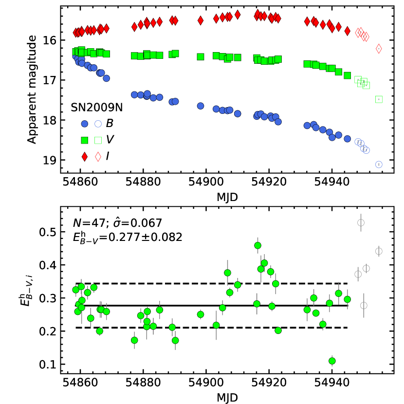
Figure 21: Top panel: $BV\!I$ light curves of SN 2009N during the plateau phase. Bottom panel: $E^{\mathrm{h}}_{{B\!-\!V},i}$ estimates obtained with the C3 method. Filled symbols are the data used to compute $E_{{B\!-\!V}}^{\mathrm{h}}$. The solid line corresponds to the $E_{{B\!-\!V}}^{\mathrm{h}}$ value that maximizes the likelihood, and dashed lines are the $\pm 1\,\hat{\sigma}$ limits around $E_{{B\!-\!V}}^{\mathrm{h}}$. Error bars are $1\,\sigma$ errors due to uncertainties on photometry.

Appendix G Spectroscopic reddening

Let a set of $N$ SN spectra $\{f_{i}\}$ corrected for $E_{{B\!-\!V}}^{\mathrm{G}}$ and $z^{\mathrm{SN}}_{\mathrm{helio}}$, where each spectrum has a dispersion $\Delta_{i}$ (in Å/pixel) and $n_{i}$ flux measurements at wavelengths $\lambda_{i,k}$ (${k=1,\ldots,n_{i}}$), and a set of $M$ reddening-free spectra $\{F_{j}\}$. For each $\{f_{i},F_{j}\}$ combination, the $E_{{B\!-\!V}}^{\mathrm{h}}$ value can be inferred minimizing

$$\hat{\sigma}_{i,j}^{2}=\frac{\Delta_{i}^{-1}}{n_{i}\!-\!2}\sum_{k}^{n_{i}}{\left[\log{\left[\frac{f_{i}(\lambda_{i,k})}{F_{j}(\lambda_{i,k})}\right]}-\!A+\frac{E_{{B\!-\!V}}^{\mathrm{h}}R_{\lambda_{i,k}}}{2.5}\right]^{2}}.$$ (69)

Here $A$ is a constant accounting for differences in SN distances and photosphere radius sizes, and $R_{\lambda}$ is the extinction curve for the host-galaxy dust along the line of sight. The best estimation for $E_{{B\!-\!V}}^{\mathrm{h}}$ is that provided by the $\{f_{i},F_{j}\}$ combination with the lowest $\hat{\sigma}_{i,j}$ value.

In this work we use the D13 and L17 spectral models as $\{F_{j}\}$, and adopt the extinction curve of Fitzpatrick (1999) with ${R_{V}=3.1}$. For an input SN we select spectra: (1) earlier that 40 d since the explosion, (2) with a minimum wavelength coverage of 360–700 nm, and (3) with differences between synthetic and observed colours lower than 0.1 mag. These criteria are such that the selected spectra are suitable to measure $E_{{B\!-\!V}}^{\mathrm{h}}$ with an error of 0.05 mag (e.g. Olivares E. et al., 2010). To be conservative, we adopt an error of 0.1 mag. For example, Fig. 22 shows the $\{f_{i},F_{j}\}$ combination for SN 2009N that minimizes equation (69). For that SN we compute $E_{{B\!-\!V}}^{\mathrm{h}}=0.202$ mag.

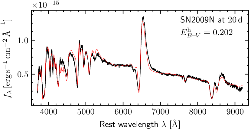
Figure 22: Spectrum of SN 2009N (corrected for $E_{{B\!-\!V}}^{\mathrm{G}}$ and $z^{\mathrm{SN}}_{\mathrm{helio}}$, black line) and model (reddened for $E_{{B\!-\!V}}^{\mathrm{h}}=0.202$ mag, red line) that minimizes equation (69).

Appendix H Magnitude transformations

We present magnitude transformations between Sloan and Johnson–Kron–Cousins filters, and between $r_{\mathrm{ZTF}}$ and $R$. All magnitudes are corrected for $E_{{B\!-\!V}}^{\mathrm{G}}$, $E_{{B\!-\!V}}^{\mathrm{h}}$, and $K$-correction, while reported uncertainties are $1\,\hat{\sigma}$ errors.

Using 12 SNe in out set having $V\!RI$ and $ri$ photometry in the radioactive tail (see Table 14), we find that $r\!-\!R$ and $i\!-\!I$ have a small linear dependence on ${V\!-\!I}$, i.e.,

$$c_{y}=a+b({V\!-\!I}),$$ (70)

where $c_{y}=r\!-\!R,i\!-\!I$. Fig. 23 shows the mean $r\!-\!R$ ($\langle r\!-\!R\rangle$) and $i\!-\!I$ ($\langle i\!-\!I\rangle$) values of each SN as a function of the mean ${V\!-\!I}$ ($\langle{V\!-\!I}\rangle$). The average of equation (70) is $\langle c_{y}\rangle=a+b\langle{V\!-\!I}\rangle$, so we can compute $a$ and $b$ fitting a straight line to the data plotted in the figure. We obtain

$$r-R=0.17({V\!-\!I})-0.03\pm 0.08$$ (71)

and

$$i-I=0.12({V\!-\!I})+0.38\pm 0.10.$$ (72)

Using the same technique for $V\!-\!R$ versus ${V\!-\!I}$ during the photospheric phase (69 SNe, Fig. 23), we obtain

$$V\!-\!R=0.59({V\!-\!I})+0.05\pm 0.05.$$ (73)

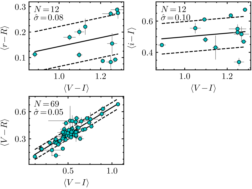
Figure 23: Upper-left (upper-right) panel: mean $r\!-\!R$ ($i\!-\!I$) against mean ${V\!-\!I}$ for 12 normal SNe II during the radioactive tail. Bottom panel: mean $V\!-\!R$ versus mean ${V\!-\!I}$ for 69 normal SNe II during the photospheric phase. Solid and dashed lines are straight line fits and $\pm 1\,\hat{\sigma}$ limits, respectively. Error bars are $1\,\sigma$ errors.

To convert $r$ to $R$ magnitudes near the maximum light, we use 18 SNe with $r\!R$ photometry at $\Delta t<20$ d (see Table 14). We find that $r\!-\!R$ is consistent with a constant value of $r\!-\!R=0.12\pm 0.08$ mag (see Fig. 24(a)).

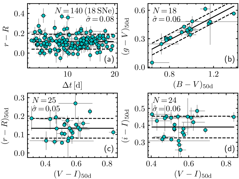
Figure 24: Panel (a): $r\!-\!R$ versus time since explosion for ${\Delta t<20}$ d. Panel (b): $g\!-\!V$ against $B\!-\!V$ at $\Delta t=50$ d. Panels (c) and (d): $r\!-\!R$ and $i\!-\!I$ versus ${V\!-\!I}$ at $\Delta t=50$ d, respectively. Solid and dashed lines are the best fits and the $\pm 1\,\hat{\sigma}$ limits, respectively. Error bars are $1\,\sigma$ errors.

To compute conversions between magnitudes at ${\Delta t=50}$ d we use 18, 25, and 24 SNe for $g/V$, $r/R$, and $i/I$ transformations, respectively. We find $(g\!-\!V)_{50\mathrm{d}}=-0.20+0.61(B\!-\!V)_{50\mathrm{d}}\pm 0.06$ (see Fig 24(b)), while the ${(r\!-\!R)_{50\mathrm{d}}}$ and ${(i\!-\!I)_{50\mathrm{d}}}$ values are consistent with constant values of $0.13\pm 0.05$ and $0.39\pm 0.06$, respectively (see Fig 24(c)-(d)).

The public ZTF photometry is not in the SDSS photometric system but in the native ZTF one, so we cannot just adopt $r_{\mathrm{ZTF}}=r$. To assess how similar the $r_{\mathrm{ZTF}}$ photometry is to the $r$- and $R$-band photometry, we compute synthetic magnitudes (Appendix A) using SN spectra. From the spectra of the SNe in our set, we select those having differences between synthetic and observed $V\!-\!r$, $V\!-\!R$, $V\!-\!i$, and/or ${V\!-\!I}$ colours lower than 0.1 mag.

The left-hand panels of Fig. 25 show the $r_{\mathrm{ZTF}}\!-\!r$ (top panel) and $r_{\mathrm{ZTF}}\!-\!R$ (bottom panel) values, computed with 308 spectra of 36 SNe during the photospheric and transition phase, against the time since explosion. We see that the $r_{\mathrm{ZTF}}\!-\!R$ values have a lower dependence on time and a lower scatter than the $r_{\mathrm{ZTF}}\!-\!r$ estimates (the $y$-axis scale is the same in the two panels). Therefore, the $r_{\mathrm{ZTF}}$ light curves during the photospheric and transition phase are more similar to the $R$-band light curves than the $r$-band ones. Given the low $\hat{\sigma}$ value (0.008 mag) around the mean ${r_{\mathrm{ZTF}}\!-\!R}$ (0.138 mag), we consider the time dependence to be negligible and adopt ${r_{\mathrm{ZTF}}\!-\!R=0.138\pm 0.008}$ mag to transform $r_{\mathrm{ZTF}}$ into $R$ magnitudes. We find similar results for the radioactive tail (right-hand panels, using 56 spectra of 13 SNe), for which we adopt $r_{\mathrm{ZTF}}\!-\!R=0.142\pm 0.024$ mag.

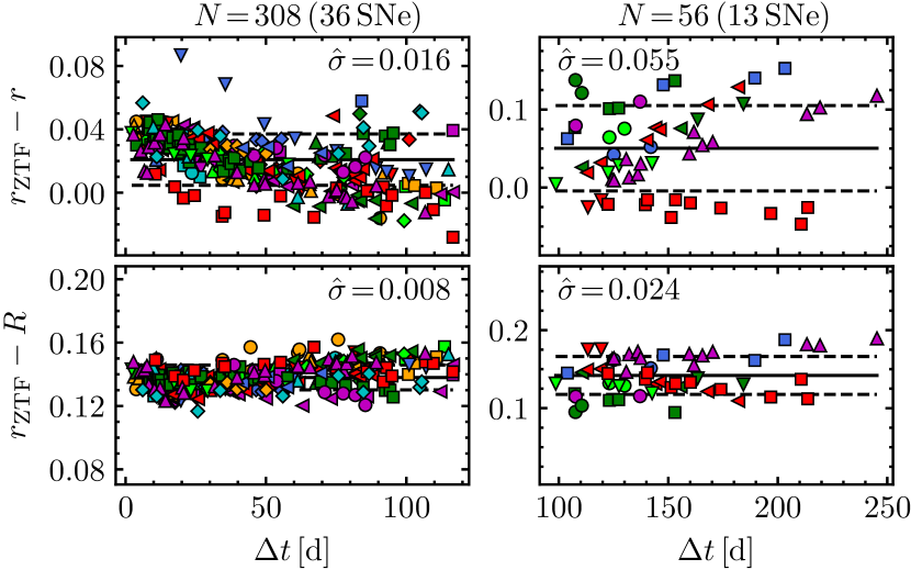
Figure 25: $r_{\mathrm{ZTF}}\!-\!r$ (top panels) and $r_{\mathrm{ZTF}}\!-\!R$ (bottom panels) values computed from spectra of normal SNe II in the photospheric and transition phase (left-hand panels) and in the radioactive tail (right-hand panels), against the time since explosion. Solid and dashed lines are mean values and $\pm 1\,\hat{\sigma}$ limits, respectively.

In the literature we find only one normal SN II having $r_{\mathrm{ZTF}}$ and $R$ photometry (SN 2018aoq; Tsvetkov et al. 2019). For that SN we measure a mean ${r_{\mathrm{ZTF}}\!-\!R}$ of $0.17\pm 0.04$ mag (16 points in the photospheric phase), which is consistent within its error with our result from synthetic magnitudes.

Appendix I $K$-corrections

We express the $x$-band $K$-correction ($K_{x,j}$) such that the apparent magnitude ($m_{x,j}$) corrected for $K$-correction is ${m_{x,j}^{K}=m_{x,j}-K_{x,j}}$, where

$$K_{x,j}=-2.5\log(1+z^{\mathrm{SN}}_{\mathrm{helio}})+k_{x,j}^{s},$$ (74)

being

$$k_{x,j}^{s}=2.5\log\left(\frac{d\lambda S_{x,\lambda}\lambda f_{j,\lambda}}{d\lambda^{\prime}S_{x,\lambda}\lambda^{\prime}f_{j,\lambda^{\prime}}}\right)$$ (75)

and $\lambda^{\prime}=\lambda/(1+z^{\mathrm{SN}}_{\mathrm{helio}})$. To compute $k_{x}^{s}$ we use the spectral models of D13, J14, and L17, and $z^{\mathrm{SN}}_{\mathrm{helio}}$ values uniformly distributed between 0.001 and 0.043. Expressing $k_{x}^{s}$ as polynomials on $\Delta t$, we obtain

$$k_{x,j}^{s}=\left(\sum_{i=0}k_{i}\cdot\left[\frac{\Delta t_{j}}{100\,\mathrm{d}}\right]^{i}\pm\hat{\sigma}\right)z^{\mathrm{SN}}_{\mathrm{helio}}.$$ (76)

Table 13 lists the parameters for the photospheric and radioactive tail phase. At ${\Delta t=200}$ d (the midpoint of the time range we use to estimate $M_{{}^{56}\mathrm{Ni}}$) $K_{x}$ values are ${<0.03}$ mag for $z^{\mathrm{SN}}_{\mathrm{helio}}=0.009$ (the median redshift in our set), while for ${z^{\mathrm{SN}}_{\mathrm{helio}}>0.02}$ (15 out of 110 SNe in our sample) $K_{x}$ values start to be comparable to the typical photometry errors.

Table 13: $K$-correction parameters.

$x$	$k_{0}^{*}$	$k_{1}^{*}$	$k_{2}^{*}$	$\hat{\sigma}^{*}$	$k_{0}^{\dagger}$	$k_{1}^{\dagger}$	$\hat{\sigma}^{\dagger}$
$B$	$-1.50$	19.8	$-10.8$	1.32	–	–	–
$g$	$-1.23$	16.1	$-10.2$	0.90	–	–	–
$V$	$-1.46$	8.85	$-5.27$	0.66	8.10	$-1.69$	2.97
$r$	$-0.05$	6.56	$-4.12$	0.72	4.12	$0.88$	2.21
$r_{\mathrm{ZTF}}$	$-0.70$	4.21	$-2.54$	0.24	0.60	$0.77$	1.22
$R$	$-0.42$	3.56	$-2.09$	0.21	1.48	$0.57$	0.92
$i$	$-1.05$	2.33	$-0.87$	0.37	1.05	$0.26$	1.00
$I$	$-1.00$	3.60	$-1.50$	0.24	6.31	$-1.69$	1.07
Note. Parameters for the photospheric ($*$) and radioactive tail ($\dagger$) phase.

Appendix J Indirect Steepness value

In order to calculate $S_{x}$ indirectly from steepnesses in bands other than $x$, we compute steepness transformations.

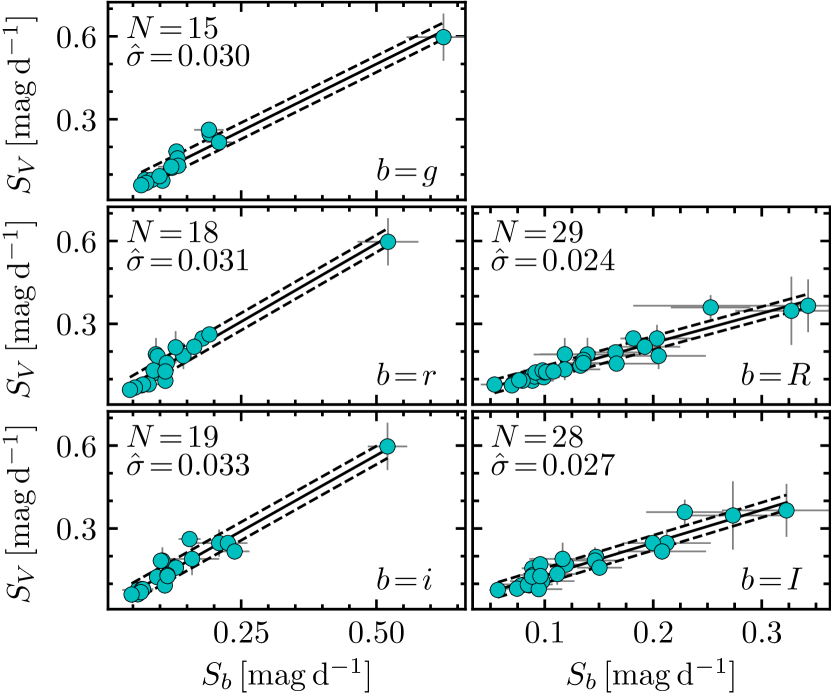
Figure 26: $V$-band steepness against the steepness for the $gr\!RiI$ bands. Solid lines are straight-line fits to the data, while dashed ones are $\pm 1\,\hat{\sigma}$ limits around the fits. Error bars are $1\,\sigma$ errors.

Fig. 26 shows $S_{V}$ against the steepness for $gr\!RiI$ bands. Using the model selection procedure (Appendix C), we find that the five correlations plotted in the figure are well represented by straight lines. In general, for the 30 possible combinations with the $gV\!r\!RiI$ bands, we find that correlations between the $x$- and $b$-band steepness are given by

$$S_{x}=c_{x,b}+d_{x,b}S_{b}.$$ (77)

Table 23 reports the $c_{x,b}$ and $d_{x,b}$ parameters, their bootstrap errors, and the $\hat{\sigma}_{x,b}$ values.

For an SN with a set of $n$ steepness estimates, $\{S_{b}\}_{b\neq x}$, we can compute a set of $n$ $S_{x}$ values, $\{S_{x}\}$, using equation (77). Our best indirect measurement of $S_{x}$ will be the weighted mean of the $\{S_{x}\}$ values, $S_{x}^{*}$, given by

$$S_{x}^{*}=\frac{1}{\sum_{b\neq x}w_{x,b}}\sum_{b\neq x}(c_{x,b}+d_{x,b}S_{b})w_{x,b},$$ (78)

where $w_{x,b}=[d_{x,b}^{2}\sigma_{S_{b}}^{2}+\hat{\sigma}_{x,b}^{2}]^{-1}$. The error on $S_{x}^{*}$ is simply

$$\sigma_{S_{x}^{*}}=\sqrt{\frac{1}{\sum_{b\neq x}w_{x,b}}}.$$ (79)

Appendix K Reference list for the data

Here the references for Tables 14, 16, 17, and 18.

(1) Barbon et al. (1982); (2) Buta (1982); (3) Tsvetkov (1983); (4) Pennypacker et al. (1989); (5) Ruiz-Lapuente et al. (1990); (6) Benetti et al. (1991); (7) Turatto et al. (1993); (8) Schmidt et al. (1993); (9) Benetti et al. (1994); (10) Cappellaro et al. (1995); (11) Blanton et al. (1995); (12) Galbany et al. (2016); (13) Clocchiatti et al. (1996); (14) Pastorello et al. (2004); (15) Inserra et al. (2013); (16) Benetti et al. (2001); (17) Elmhamdi et al. (2003a); (18) Krisciunas et al. (2009); (19) Faran et al. (2014a); (20) Rubenstein (1999); (21) Pastorello et al. (2009b); (22) Leonard et al. (2002); (23) Pozzo et al. (2006); (24) Tsvetkov et al. (2007); (25) Spiro et al. (2014); (26) Hendry et al. (2005); (27) Faran et al. (2014b); (28) Gurugubelli et al. (2008); (29) Zhang et al. (2006); (30) Vinkó et al. (2006); (31) Vinkó et al. (2009); (32) Meikle et al. (2011); (33) Anderson et al. (2014); (34) Sahu et al. (2006); (35) Misra et al. (2007); (36) Maguire et al. (2010); (37) Arcavi et al. (2012); (38) Tsvetkov et al. (2006); (39) Dessart et al. (2008); (40) Pastorello et al. (2009a); (41) Hicken et al. (2017); (42) Brown et al. (2009); (43) Andrews et al. (2011); (44) Andrews et al. (2010); (45) Inserra et al. (2011); (46) de Jaeger et al. (2019); (47) Van Dyk et al. (2012); (48) Van Dyk (2013); (49) Pignata (2013); (50) Roy et al. (2011a); (51) Roy et al. (2011b); (52) Takáts et al. (2014); (53) Tsvetkov (2014); (54) Inserra et al. (2012); (55) Elias-Rosa et al. (2011); (56) Takáts et al. (2015); (57) Fraser et al. (2011); (58) Rubin et al. (2016); (59) Tomasella et al. (2013); (60) Bayless et al. (2013); (61) Bose et al. (2013); (62) Munari et al. (2013); (63) Dall’Ora et al. (2014); (64) Barbarino et al. (2015); (65) Tomasella et al. (2018); (66) Bose et al. (2015a); (67) Zhang et al. (2014); (68) Valenti et al. (2016); (69) Valenti et al. (2015); (70) Richmond (2014); (71) Bose et al. (2015b); (72) Huang et al. (2015); (73) Dhungana et al. (2016); (74) Yuan et al. (2016); (75) Bullivant et al. (2018); (76) Bose et al. (2016); (77) Terreran et al. (2016); (78) Huang et al. (2016); (79) Dastidar et al. (2021); (80) Singh et al. (2018); (81) Wyrzykowski et al. (2014); (82) Dastidar et al. (2019); (83) Dastidar et al. (2018); (84) Bostroem et al. (2019); (85) Huang et al. (2018); (86) Bose et al. (2019); (87) Müller-Bravo et al. (2020); (88) Nakaoka et al. (2018); (89) Hosseinzadeh et al. (2018); (90) Singh et al. (2019); (91) Tartaglia et al. (2018); (92) Afsariardchi et al. (2019); (93) Tartaglia et al. (2021); (94) Rho et al. (2018); (95) Tsvetkov et al. (2018); (96) Tinyanont et al. (2019); (97) Van Dyk et al. (2019); (98) Szalai et al. (2019); (99) Buta & Keel (2019); (100) Andrews et al. (2019); (101) Dong et al. (2020); (102) Reguitti et al. (2021); (103) Anand et al. (2018); (104) de Jaeger et al. (2020); (105) Riess et al. (2016); (106) McQuinn et al. (2017); (107) Freedman et al. (2019); (108) Saha et al. (2006); (109) Carlin et al. (2016); (110) Monachesi et al. (2016); (111) Zgirski et al. (2017); (112) Jang & Lee (2017); (113) Rizzi et al. (2007); (114) Tikhonov & Galazutdinova (2020); (115) Hamuy (2001); (116) Rodríguez et al. (2014); (117) Olivares E. et al. (2010); (118) Turatto et al. (1998); (119) Pastorello et al. (2006); (120) Quimby et al. (2007); (121) Li et al. (2007); (122) Yaron et al. (2017); (123) Childress et al. (2016); (124) Thompson (1982); (125) Gutiérrez et al. (2017a); (126) Harutyunyan et al. (2008); (127) Hendry et al. (2006); (128) Shivvers et al. (2017); (129) Liao et al. (2019); (130) Itagaki (2016); (131) Dimai (2016); (132) Wiggins (2017).

Appendix L Tables

Table 14: SN sample.

SN	Host galaxy	$E_{{B\!-\!V}}^{\mathrm{G}}$	$cz^{\mathrm{SN}}_{\mathrm{helio}}$	$\mu$	$E_{{B\!-\!V}}^{\mathrm{h}}$	$t_{0}$	References
		(mag)	(km s-1)	(mag)	(mag)	(MJD)
1980K	NGC 6946	0.291	$40$	$29.44\pm 0.09$	$-0.106\pm 0.084$	$44528.2\pm 5.9$	1, 2, 3
1986I	M99	0.034	$2407$	$30.71\pm 0.40$	$0.212\pm 0.142$	$46556.4\pm 1.9$	4
1988A	M58	0.035	$1517$	$31.17\pm 0.35$	$0.090\pm 0.111$	$47176.2\pm 0.3$	5, 6, 7
1990E	NGC 1035	0.022	$1362$	$30.83\pm 0.26$	$0.598\pm 0.072$	$47934.4\pm 1.4$	8, 9
1990K	NGC 150	0.012	$1584$	$31.57\pm 0.24$	$0.227\pm 0.034$	$48013.8\pm 4.2$	10
1991G	NGC 4088	0.017	$757$	$30.76\pm 0.17$	$0.025\pm 0.071$	$48281.5\pm 5.3$	11
1991al	LEDA 140858	0.044	$4572$	$32.80\pm 0.12$	$0.067\pm 0.026$	$48446.7\pm 3.7$	12
1992H	NGC 5377	0.015	$1793$	$32.07\pm 0.17$	$0.167\pm 0.123$	$48656.4\pm 4.5$	13
1992ba	NGC 2082	0.050	$1135$	$30.78\pm 0.29$	$0.096\pm 0.029$	$48886.1\pm 2.8$	12
1994N	UGC 5695	0.032	$2940$	$33.24\pm 0.20$	$0.045\pm 0.036$	$49453.9\pm 4.5$	14
1995ad†	NGC 2139	0.029	$1837$	$32.24\pm 0.18$	$0.090\pm 0.111$	$49972.0\pm 4.2$	15
1996W	NGC 4027	0.036	$1617$	$31.86\pm 0.19$	$0.260\pm 0.054$	$50180.2\pm 2.5$	15
1997D	NGC 1536	0.017	$1217$	$30.93\pm 0.25$	$0.090\pm 0.111$	$50361.0\pm 15.0$	16
1999ca	NGC 3120	0.094	$2791$	$32.82\pm 0.11$	$0.076\pm 0.033$	$51273.4\pm 2.9$	12
1999em†	NGC 1637	0.035	$800$	$30.31\pm 0.09$	$0.082\pm 0.034$	$51474.5\pm 2.0$	12, 17, 18, 19
1999ga	NGC 2442	0.173	$1466$	$31.51\pm 0.05$	$0.511\pm 0.084$	$51419.5\pm 20.0$	20, 21
1999gi	NGC 3184	0.014	$503$	$30.40\pm 0.18$	$0.250\pm 0.033$	$51518.6\pm 1.8$	19, 22
2001X	NGC 5921	0.034	$1480$	$31.52\pm 0.21$	$0.063\pm 0.031$	$51963.6\pm 2.6$	19
2001dc	NGC 5777	0.009	$2145$	$32.69\pm 0.16$	$0.694\pm 0.076$	$52046.0\pm 5.0$	14
2002gw	NGC 922	0.016	$3143$	$32.98\pm 0.22$	$0.138\pm 0.036$	$52554.8\pm 3.0$	12
2002hh	NGC 6946	1.065	$110$	$29.44\pm 0.09$	$1.545\pm 0.182$	$52575.6\pm 2.5$	23, 24
2002hx	PGC 23727	0.045	$9299$	$35.53\pm 0.08$	$0.140\pm 0.043$	$52580.3\pm 3.7$	12
2003B	NGC 1097	0.023	$1141$	$30.62\pm 0.25$	$0.023\pm 0.033$	$52622.2\pm 4.2$	12
2003T	UGC 4864	0.027	$8368$	$35.33\pm 0.10$	$0.154\pm 0.040$	$52652.6\pm 4.6$	12
2003Z	NGC 2742	0.033	$1289$	$31.62\pm 0.23$	$0.109\pm 0.050$	$52665.1\pm 2.4$	19, 25
2003fb	UGC 11522	0.155	$5081$	$34.05\pm 0.13$	$0.371\pm 0.046$	$52779.0\pm 4.4$	12
2003gd	M74	0.060	$657$	$29.95\pm 0.08$	$0.144\pm 0.040$	$52716.5\pm 21.0$	12, 19, 26
2003hd	ESO 543-G17	0.011	$12031$	$35.97\pm 0.08$	$0.124\pm 0.042$	$52857.2\pm 2.8$	12
2003hk	NGC 1085	0.032	$6880$	$34.77\pm 0.12$	$0.142\pm 0.054$	$52868.3\pm 2.7$	12, 27
2003hn†	NGC 1448	0.012	$1305$	$31.31\pm 0.04$	$0.169\pm 0.040$	$52865.6\pm 4.0$	12, 18
2003ho	ESO 235-G58	0.033	$4091$	$33.70\pm 0.18$	$0.640\pm 0.050$	$52848.5\pm 3.3$	12
2003iq	NGC 772	0.062	$2331$	$32.41\pm 0.16$	$0.122\pm 0.038$	$52919.4\pm 0.9$	12, 19
2004A	NGC 6207	0.013	$852$	$30.87\pm 0.26$	$0.177\pm 0.043$	$53012.5\pm 1.7$	28
2004dj†	NGC 2403	0.034	$221$	$27.46\pm 0.11$	$0.094\pm 0.035$	$53180.6\pm 15.6$	29, 30, 31, 32
2004eg	UGC 3053	0.390	$2414$	$32.46\pm 0.24$	$0.160\pm 0.150$	$53169.5\pm 30.0$	25
2004ej	NGC 3095	0.060	$2723$	$32.76\pm 0.13$	$0.145\pm 0.116$	$53231.5\pm 4.2$	33
2004et†	NGC 6946	0.293	$40$	$29.44\pm 0.09$	$0.073\pm 0.043$	$53270.5\pm 0.3$	19, 34, 35, 36
2004fx	MCG -02-14-3	0.088	$2673$	$32.73\pm 0.19$	$0.090\pm 0.115$	$53305.1\pm 1.4$	33
2005af	NGC 4945	0.159	$563$	$27.75\pm 0.12$	$0.090\pm 0.117$	$53320.8\pm 17.0$	33
2005au	NGC 5056	0.010	$5592$	$34.43\pm 0.12$	$0.117\pm 0.073$	$53441.4\pm 6.1$	37
2005ay	NGC 3938	0.018	$850$	$30.68\pm 0.21$	$0.035\pm 0.037$	$53450.7\pm 1.8$	19, 38
2005cs†∗	M51a	0.032	$463$	$29.67\pm 0.07$	$0.124\pm 0.037$	$53548.4\pm 0.3$	19, 38, 39, 40
2005dx	ESO 550-G2	0.021	$8012$	$35.09\pm 0.09$	$0.090\pm 0.142$	$53615.7\pm 4.6$	33
2006my	NGC 4651	0.012	$788$	$31.40\pm 0.10$	$-0.062\pm 0.152$	$53942.5\pm 20.0$	36
2006ov‡	M61	0.019	$1566$	$31.40\pm 0.63$	$0.275\pm 0.105$	$53973.5\pm 6.0$	25, 41
2007aa	NGC 4030	0.023	$1574$	$31.99\pm 0.27$	$0.046\pm 0.100$	$54131.9\pm 4.1$	33, 41, 42
2007hv	UGC 2858	0.418	$5054$	$34.05\pm 0.16$	$0.000\pm 0.100$	$54346.6\pm 2.8$	41
2007it	NGC 5530	0.099	$1193$	$30.56\pm 0.24$	$0.109\pm 0.111$	$54348.0\pm 0.6$	33, 43
2007od	UGC 12846	0.031	$1734$	$31.63\pm 0.25$	$0.134\pm 0.070$	$54388.2\pm 4.1$	41, 44, 45, 46
2008K	ESO 504-G4	0.033	$7964$	$35.29\pm 0.10$	$0.090\pm 0.111$	$54466.8\pm 4.8$	33
2008M	ESO 121-G26	0.039	$2192$	$32.62\pm 0.20$	$0.090\pm 0.112$	$54475.3\pm 3.3$	33
2008aw	NGC 4939	0.035	$3110$	$33.19\pm 0.17$	$0.226\pm 0.043$	$54519.3\pm 3.9$	33
2008bk†	NGC 7793	0.017	$230$	$27.66\pm 0.08$	$0.090\pm 0.111$	$54547.1\pm 2.6$	47, 48, 49
2008gz	NGC 3672	0.036	$1862$	$32.22\pm 0.15$	$-0.031\pm 0.040$	$54693.5\pm 5.0$	50
2008in†‡∗	M61	0.019	$1566$	$31.40\pm 0.63$	$0.037\pm 0.044$	$54824.2\pm 0.1$	41, 46, 51
2009N‡∗	NGC 4487	0.018	$905$	$30.90\pm 0.38$	$0.265\pm 0.045$	$54850.1\pm 3.4$	41, 46, 52
2009at	NGC 5301	0.015	$1503$	$31.82\pm 0.22$	$0.551\pm 0.079$	$54899.1\pm 2.0$	46
2009ay	NGC 6479	0.034	$6650$	$34.74\pm 0.13$	$0.252\pm 0.087$	$54898.3\pm 4.4$	41, 46, 53
2009bw†	UGC 2890	0.197	$1155$	$31.07\pm 0.26$	$0.160\pm 0.049$	$54916.5\pm 3.0$	54
2009dd	NGC 4088	0.017	$757$	$30.76\pm 0.17$	$0.285\pm 0.057$	$54916.0\pm 4.2$	15, 41
2009hd	M66	0.029	$727$	$30.15\pm 0.07$	$1.206\pm 0.056$	$55001.6\pm 3.9$	55
2009ib∗	NGC 1559	0.026	$1304$	$31.41\pm 0.05$	$0.147\pm 0.038$	$55040.3\pm 4.0$	56
2009md†	NGC 3389	0.023	$1308$	$32.06\pm 0.12$	$0.165\pm 0.048$	$55161.9\pm 7.9$	57
2010aj	MCG -01-32-35	0.029	$6497$	$34.78\pm 0.12$	$0.082\pm 0.048$	$55261.8\pm 3.5$	15, 41
PTF10gva	NSA 49030	0.026	$8253$	$35.33\pm 0.10$	$0.111\pm 0.111$	$55320.3\pm 0.9$	58
2011fd	NGC 2273B	0.063	$2101$	$32.41\pm 0.22$	$0.090\pm 0.111$	$55777.9\pm 4.5$	46
PTF11go	MCG +09-19-105	0.010	$8037$	$35.22\pm 0.10$	$0.160\pm 0.150$	$55570.9\pm 1.4$	58
PTF11htj	SDSS J211603.12+123124.4	0.060	$5096$	$34.04\pm 0.15$	$0.160\pm 0.150$	$55751.9\pm 1.5$	58
PTF11izt	anonymous	0.047	$5996$	$34.52\pm 0.11$	$0.160\pm 0.150$	$55766.8\pm 1.3$	58
2012A∗	NGC 3239	0.027	$753$	$30.66\pm 0.24$	$0.040\pm 0.049$	$55929.3\pm 2.6$	46, 59
2012aw∗	M95	0.024	$778$	$29.93\pm 0.05$	$0.115\pm 0.041$	$56002.0\pm 0.5$	46, 60, 61, 62, 63
2012br	SDSS J122417.04+185529.4	0.031	$6805$	$34.90\pm 0.12$	$0.199\pm 0.260$	$56000.9\pm 0.2$	58
2012cd	CGCG 271-34	0.025	$3525$	$33.54\pm 0.19$	$0.123\pm 0.134$	$56019.4\pm 1.9$	58
2012ec†‡∗	NGC 1084	0.023	$1407$	$31.07\pm 0.25$	$0.102\pm 0.048$	$56144.5\pm 3.4$	46, 64
PTF12grj	WISEA J012039.07+044621.5	0.024	$10193$	$35.62\pm 0.09$	$0.160\pm 0.150$	$56123.4\pm 0.6$	58
PTF12hsx	SDSS J005503.33+421954.0	0.079	$5696$	$34.34\pm 0.14$	$0.167\pm 0.221$	$56113.0\pm 0.5$	58
2013K	ESO 9-G10	0.122	$2418$	$32.48\pm 0.21$	$0.512\pm 0.066$	$56294.5\pm 4.2$	65
2013ab‡∗	NGC 5669	0.023	$1368$	$31.38\pm 0.20$	$0.028\pm 0.040$	$56339.6\pm 0.6$	46, 66
2013am∗	M65	0.021	$1114$	$30.36\pm 0.29$	$0.536\pm 0.069$	$56371.8\pm 0.4$	46, 65, 67
2013bu	NGC 7331	0.078	$440$	$30.84\pm 0.10$	$0.523\pm 0.062$	$56396.6\pm 2.0$	46, 68

Table 15: continued

SN	Host galaxy	$E_{{B\!-\!V}}^{\mathrm{G}}$	$cz^{\mathrm{SN}}_{\mathrm{helio}}$	$\mu$	$E_{{B\!-\!V}}^{\mathrm{h}}$	$t_{0}$	References
		(mag)	(km s-1)	(mag)	(mag)	(MJD)
2013by	ESO 138-G10	0.188	$1144$	$30.46\pm 0.29$	$0.196\pm 0.100$	$56401.6\pm 3.6$	69
2013ej†‡∗	M74	0.060	$657$	$29.95\pm 0.08$	$0.044\pm 0.040$	$56496.8\pm 0.2$	46, 70, 71, 72, 73, 74
2013fs∗	NGC 7610	0.035	$3554$	$33.32\pm 0.18$	$0.027\pm 0.037$	$56570.8\pm 0.5$	68, 75
2013hj	MCG -02-24-3	0.045	$2072$	$32.51\pm 0.13$	$0.047\pm 0.039$	$56636.8\pm 0.9$	76
iPTF13dkz	SDSS J013611.64+333703.6	0.039	$4797$	$33.85\pm 0.17$	$0.144\pm 0.180$	$56547.9\pm 0.3$	58
LSQ13dpa	LCSB S1492O	0.032	$7045$	$35.00\pm 0.11$	$0.160\pm 0.150$	$56642.2\pm 2.0$	68
2014G†‡∗	NGC 3448	0.010	$1160$	$31.96\pm 0.14$	$0.268\pm 0.046$	$56669.3\pm 0.8$	46, 76, 77
2014cx‡∗	NGC 337	0.096	$1646$	$31.51\pm 0.22$	$-0.021\pm 0.045$	$56901.9\pm 0.3$	78
2014cy∗	NGC 7742	0.048	$1663$	$31.54\pm 0.23$	$0.090\pm 0.045$	$56899.6\pm 0.7$	46, 68, 79
2014dw	NGC 3568	0.092	$2444$	$32.39\pm 0.13$	$0.182\pm 0.127$	$56957.5\pm 10.0$	68
ASASSN-14dq‡	UGC 11860	0.060	$3125$	$32.97\pm 0.21$	$0.108\pm 0.038$	$56841.0\pm 5.5$	80
ASASSN-14ha	NGC 1566	0.008	$1504$	$30.86\pm 0.15$	$0.090\pm 0.111$	$56909.5\pm 0.6$	68
OGLE14-18	ESO 87-G3	0.049	$8082$	$35.18\pm 0.10$	$0.144\pm 0.137$	$56701.7\pm 0.9$	81
2015V	UGC 11000	0.031	$1369$	$31.63\pm 0.22$	$0.031\pm 0.060$	$57112.3\pm 4.3$	46
2015W	UGC 3617	0.118	$3984$	$33.70\pm 0.19$	$0.157\pm 0.063$	$57015.0\pm 6.5$	46, 68
2015an	IC 2367	0.009	$2448$	$32.79\pm 0.13$	$0.114\pm 0.111$	$57268.0\pm 1.6$	82
2015ba	IC 1029	0.015	$2383$	$32.80\pm 0.16$	$0.416\pm 0.047$	$57347.5\pm 4.9$	83
2015cz	NGC 582	0.045	$4352$	$33.68\pm 0.16$	$0.472\pm 0.065$	$57290.4\pm 7.5$	79
ASASSN-15oz	LEDA 4614833	0.078	$2078$	$31.90\pm 0.26$	$0.230\pm 0.056$	$57259.1\pm 1.9$	84
2016X‡∗	UGC 8041	0.019	$1321$	$31.32\pm 0.34$	$0.079\pm 0.049$	$57405.9\pm 0.3$	46, 85, 86
2016aqf	NGC 2101	0.047	$1204$	$31.01\pm 0.25$	$0.180\pm 0.100$	$57442.6\pm 0.3$	87
2016bkv∗	NGC 3184	0.014	$592$	$30.40\pm 0.18$	$0.036\pm 0.078$	$57467.5\pm 1.2$	88, 89
2016gfy	NGC 2276	0.086	$2416$	$32.64\pm 0.22$	$0.163\pm 0.045$	$57641.3\pm 2.6$	90
2016ija	NGC 1532	0.013	$1040$	$30.55\pm 0.17$	$1.950\pm 0.150$	$57712.1\pm 1.0$	91
2017it	anonymous	0.029	$12891$	$36.21\pm 0.07$	$-0.087\pm 0.042$	$57746.2\pm 0.7$	92
2017ahn	NGC 3318	0.067	$2775$	$32.84\pm 0.10$	$0.233\pm 0.148$	$57791.8\pm 0.5$	93
2017eaw†‡∗	NGC 6946	0.293	$40$	$29.44\pm 0.09$	$0.059\pm 0.037$	$57886.2\pm 0.6$	94, 95, 96, 97, 98, 99
2017gmr†‡∗	NGC 988	0.023	$1510$	$31.08\pm 0.19$	$0.332\pm 0.045$	$57999.2\pm 0.6$	100
2018cuf	IC 5092	0.028	$3248$	$33.10\pm 0.19$	$0.221\pm 0.100$	$58291.8\pm 0.3$	101
2018hwm	IC 2327	0.022	$2684$	$33.08\pm 0.19$	$0.150\pm 0.069$	$58424.8\pm 0.9$	102
Notes. Column 1: SN names. Column 2: SN host galaxy names, Column 3: Galactic colour excesses with random errors of 16 per cent. Column 4: heliocentric SN redshifts. Column 5 and 6: host galaxy distance moduli and colour excesses, respectively. Column 7: explosion epochs. Column 8: references for the photometry (codes are in Appendix K).
†Selected to compute BCs.
‡With $V\!RI$ and $ri$ photometry in the radioactive tail.
∗Used to compute $r\!-\!R$ for $\Delta t<20$ d.

Table 16: Host galaxy distance moduli. The full table is available online as supplementary data.

Host galaxy	SN	$\mu_{\mathrm{CPL}}$	$\mu_{\mathrm{TRGB}}$	$\mu_{\mathrm{TF}}$	$\mu_{\mathrm{HLL}}$	$\mu_{\mathrm{SVF}}$	$\mu$
NGC 6946	1980K	–	$29.44\pm 0.09^{103}$	–	–	–	$29.44\pm 0.09$
	2002hh	–	–	–	–	–	$29.44\pm 0.09$
	2004et	–	–	–	–	–	$29.44\pm 0.09$
Notes. Column 1: SN host galaxy names. Column 2: SN names, Columns 3 and 4: Cepheids and TRGB distances from the literature, respectively. Column 5: Tully-Fisher distances from EDD. Column 6: distances compute with the Hubble-Lemaître law. Column 6: distances inferred from smoothed velocity fields (Kourkchi et al., 2020). Column 8: adopted distance moduli. References for the data (superscript numbers) are in Appendix K.

Table 17: Host galaxy colour excesses. The full table is available online as supplementary data.

SN	$E_{{B\!-\!V}}^{\mathrm{h,C3}}$	$E_{{B\!-\!V}}^{\mathrm{h},{V\!-\!I}}$	$E_{{B\!-\!V}}^{\mathrm{h,spec}}$	$E_{{B\!-\!V}}^{\mathrm{h,NaID}}$	$E_{{B\!-\!V}}^{\mathrm{h}}$
1980K	$-0.106\pm 0.084$	–	–	–	$0.106\pm 0.084$
1986I	–	–	–	$\phantom{-}0.122\pm 0.090^{4}$	$\phantom{-}0.212\pm 0.142$
1988A	–	–	–	$\phantom{-}0.000\pm 0.014^{115}$	$\phantom{-}0.090\pm 0.111$
Notes. Column 1: SN names. Column 2: $E_{{B\!-\!V}}^{\mathrm{h}}$ values computed with the C3 method. Column 3: $E_{{B\!-\!V}}^{\mathrm{h}}$ values measured with the ${V\!-\!I}$ colour method. Column 4: $E_{{B\!-\!V}}^{\mathrm{h}}$ computed with the spectrum-fitting technique. Column 5: $E_{{B\!-\!V}}^{\mathrm{h}}$ values estimated from the pEW of the host galaxy Na i D line. Column 6: adopted host galaxy colour excesses. References for the data (superscript numbers) are in Appendix K.

Table 18: SN explosion epochs. The full table is available online as supplementary data.

SN	$t_{\mathrm{ln}}$ (MJD)	$t_{\mathrm{fd}}$ (MJD)	$t_{0}$ (MJD)	Phase source	Spectral source
1980K	$44494.0$	$44540.0$	$44528.2\pm 5.9$	124, IAUC 3532	WISeREP
1986I	–	$46558.0$	$46556.4\pm 1.9$	IAUC 4219	4
1988A	$47175.7$	$47176.8$	$47176.2\pm 0.3$	IAUC 4533, IAUC 4540	125
Notes. Column 1: SN names. Column 2 and 3: SN last non-detection and first detection epochs, respectively. Column 4: explosion epochs estimated with the SNII_ETOS code ($\pm 1\,\hat{\sigma}$ error), unless otherwise noted. Column 5: references for $t_{\mathrm{ln}}$ and $t_{\mathrm{fd}}$. Column 6: data source of spectroscopy used to compute $t_{0}$ with the SNII_ETOS code. Reference codes are in Appendix K.

Table 19: ⁵⁶Ni masses and light-curve parameters.

SN	$x$	Range	$N$	$T_{0}$	$\log{(M_{{}^{56}\mathrm{Ni}}[\mathrm{M}_{\sun}])}$	$M_{{}^{56}\mathrm{Ni}}$	$M_{V}^{50\mathrm{d}}$	$\rho$
		(d)		(d)	(dex)	($\mathrm{M}_{\sun}$)	(mag)
1980K	$V$	100–285	9	–	$-1.462\pm 0.147$	$0.03655\pm 0.01273$	$-17.348\pm 0.379$	$-0.655$
1986I	$I$	171–213	4	–	$-1.302\pm 0.198$	$0.05535\pm 0.02661$	$-16.911\pm 0.590$	$-0.900$
1988A	$R$	185–189	3	–	$-1.109\pm 0.185$	$0.08519\pm 0.03800$	$-16.488\pm 0.488$	$-0.930$
1990E	$I$	141–300	7	–	$-1.383\pm 0.123$	$0.04309\pm 0.01245$	$-16.702\pm 0.341$	$-0.899$
1990K	$R$	100–223	7	222	$-1.470\pm 0.118$	$0.03516\pm 0.00973$	$-16.705\pm 0.275$	$-0.810$
1991G	$I$	135–303	7	–	$-1.778\pm 0.099$	$0.01711\pm 0.00395$	$-15.365\pm 0.277$	$-0.798$
1991al	$I$	101–129	4	–	$-1.629\pm 0.068$	$0.02379\pm 0.00375$	$-15.974\pm 0.159$	$-0.670$
1992H	$V$	140–292	7	–	$-0.788\pm 0.178$	$0.17721\pm 0.07579$	$-17.670\pm 0.413$	$-0.899$
1992ba	$I$	150–197	3	–	$-1.744\pm 0.126$	$0.01881\pm 0.00557$	$-15.733\pm 0.305$	$-0.925$
1994N	$R$	260–290	3	–	$-2.283\pm 0.106$	$0.00537\pm 0.00133$	$-14.955\pm 0.233$	$-0.801$
1995ad	$I$	104–229	7	258	$-1.230\pm 0.115$	$0.06099\pm 0.01644$	$-17.086\pm 0.387$	$-0.858$
1996W	$I$	250–309	3	–	$-0.952\pm 0.097$	$0.11451\pm 0.02590$	$-17.469\pm 0.256$	$-0.823$
1997D	$I$	125–176	6	–	$-2.064\pm 0.144$	$0.00912\pm 0.00311$	$<-14.436\pm 0.423$	$-0.824$
1999ca	$I$	203–223	7	–	$-1.846\pm 0.070$	$0.01444\pm 0.00234$	$-16.804\pm 0.167$	$-0.644$
1999em	$I$	132–311	11	–	$-1.296\pm 0.062$	$0.05110\pm 0.00733$	$-16.692\pm 0.138$	$-0.661$
1999ga	$I$	121–196	3	–	$-1.446\pm 0.120$	$0.03720\pm 0.01048$	$<-16.693\pm 0.285$	$-0.497$
1999gi	$I$	133–177	7	186	$-1.333\pm 0.087$	$0.04739\pm 0.00959$	$-16.250\pm 0.207$	$-0.845$
2001X	$I$	123–144	4	–	$-1.395\pm 0.097$	$0.04129\pm 0.00934$	$-16.348\pm 0.231$	$-0.877$
2001dc	$I$	119–153	7	–	$-2.119\pm 0.110$	$0.00785\pm 0.00202$	$-15.059\pm 0.283$	$-0.709$
2002gw	$I$	137–153	3	–	$-1.631\pm 0.103$	$0.02406\pm 0.00579$	$-16.017\pm 0.246$	$-0.869$
2002hh	$I$	167–286	14	–	$-1.082\pm 0.069$	$0.08385\pm 0.01341$	$-16.882\pm 0.285$	$-0.611$
2002hx	$I$	96–160	7	–	$-1.186\pm 0.064$	$0.06587\pm 0.00976$	$-16.671\pm 0.165$	$-0.612$
2003B	$I$	223–282	3	–	$-2.223\pm 0.115$	$0.00620\pm 0.00167$	$-14.768\pm 0.271$	$-0.876$
2003T	$V$	121–137	3	–	$-1.344\pm 0.101$	$0.04653\pm 0.01097$	$-16.674\pm 0.164$	$-0.595$
2003Z	$I$	151–208	3	–	$-2.262\pm 0.116$	$0.00567\pm 0.00154$	$-14.610\pm 0.277$	$-0.821$
2003fb	$V$	116–147	5	–	$-1.482\pm 0.111$	$0.03406\pm 0.00885$	$-16.016\pm 0.206$	$-0.725$
2003gd	$I$	128–301	17	303	$-1.694\pm 0.099$	$0.02076\pm 0.00480$	$<-16.405\pm 0.149$	$-0.407$
2003hd	$I$	104–138	4	–	$-1.362\pm 0.063$	$0.04391\pm 0.00640$	$-17.056\pm 0.156$	$-0.629$
2003hk	$R$	117–145	3	–	$-1.572\pm 0.105$	$0.02759\pm 0.00677$	$-17.101\pm 0.211$	$-0.635$
2003hn	$I$	121–151	8	187	$-1.412\pm 0.056$	$0.03905\pm 0.00506$	$-16.819\pm 0.136$	$-0.514$
2003ho	$R$	102–118	3	–	$-1.601\pm 0.105$	$0.02580\pm 0.00633$	$-16.554\pm 0.267$	$-0.717$
2003iq	$I$	120–126	3	–	$-1.318\pm 0.082$	$0.04895\pm 0.00933$	$-16.763\pm 0.200$	$-0.817$
2004A	$I$	122–241	21	–	$-1.604\pm 0.116$	$0.02579\pm 0.00701$	$-15.898\pm 0.291$	$-0.913$
2004dj	$I$	131–284	17	–	$-1.902\pm 0.130$	$0.01311\pm 0.00401$	$-15.846\pm 0.178$	$-0.320$
2004eg	$I$	150–203	4	–	$-2.126\pm 0.188$	$0.00822\pm 0.00373$	$<-15.077\pm 0.551$	$-0.744$
2004ej	$V$	120–194	14	–	$-1.793\pm 0.166$	$0.01733\pm 0.00687$	$-16.494\pm 0.380$	$-0.881$
2004et	$I$	135–319	23	372	$-1.037\pm 0.071$	$0.09307\pm 0.01532$	$-17.645\pm 0.213$	$-0.759$
2004fx	$V$	109–161	24	–	$-1.802\pm 0.173$	$0.01708\pm 0.00708$	$-15.720\pm 0.400$	$-0.906$
2005af	$V$	123–162	20	234	$-1.477\pm 0.179$	$0.03630\pm 0.01562$	$<-15.212\pm 0.383$	$-0.836$
2005au	$I$	102–137	5	–	$-1.195\pm 0.085$	$0.06506\pm 0.01286$	$-17.291\pm 0.273$	$-0.718$
2005ay	$R$	117–236	5	–	$-1.778\pm 0.109$	$0.01721\pm 0.00439$	$-15.512\pm 0.239$	$-0.828$
2005cs	$I$	150–311	18	–	$-2.241\pm 0.076$	$0.00583\pm 0.00103$	$-15.371\pm 0.133$	$-0.474$
2005dx	$V$	103–120	3	–	$-2.064\pm 0.194$	$0.00954\pm 0.00448$	$-15.583\pm 0.445$	$-0.878$
2006my	$I$	177–261	8	–	$-1.674\pm 0.141$	$0.02233\pm 0.00745$	$<-15.361\pm 0.473$	$-0.768$
2006ov	$I$	145–231	9	–	$-2.051\pm 0.267$	$0.01074\pm 0.00728$	$<-16.568\pm 0.707$	$-0.961$
2007aa	$i$	106–121	7	–	$-1.522\pm 0.143$	$0.03174\pm 0.01074$	$-16.556\pm 0.407$	$-0.907$
2007hv	$i$	113–131	6	–	$-1.326\pm 0.125$	$0.04920\pm 0.01446$	$-16.698\pm 0.400$	$-0.887$
2007it	$I$	137–312	7	–	$-0.987\pm 0.130$	$0.10776\pm 0.03299$	$-17.400\pm 0.417$	$-0.899$
2007od	$I$	239–316	3	–	$>-2.482\pm 0.148$	$>0.00349\pm 0.00123$	$-17.438\pm 0.332$	$-0.713$
2008K	$V$	122–182	4	–	$-1.611\pm 0.180$	$0.02669\pm 0.01155$	$-16.806\pm 0.378$	$-0.713$
2008M	$V$	96–120	5	–	$-1.605\pm 0.172$	$0.02686\pm 0.01107$	$-16.504\pm 0.396$	$-0.900$
2008aw	$V$	103–133	5	117	$-1.074\pm 0.114$	$0.08729\pm 0.02331$	$-17.228\pm 0.230$	$-0.700$
2008bk	$I$	175–292	5	–	$-2.064\pm 0.094$	$0.00883\pm 0.00193$	$-14.992\pm 0.366$	$-0.806$
2008gz	$I$	127–273	26	–	$-1.253\pm 0.081$	$0.05683\pm 0.01069$	$<-16.366\pm 0.194$	$-0.784$
2008in	$I$	113–152	9	–	$-1.640\pm 0.258$	$0.02733\pm 0.01778$	$-16.134\pm 0.644$	$-0.979$
2009N	$I$	109–191	23	–	$-1.891\pm 0.161$	$0.01377\pm 0.00528$	$-15.357\pm 0.404$	$-0.951$
2009at	$I$	115–142	3	–	$-1.750\pm 0.115$	$0.01842\pm 0.00496$	$-16.153\pm 0.332$	$-0.841$
2009ay	$R$	100–178	8	–	$-0.932\pm 0.116$	$0.12120\pm 0.03296$	$-17.720\pm 0.309$	$-0.790$
2009bw	$I$	138–235	10	236	$-1.737\pm 0.120$	$0.01904\pm 0.00536$	$-16.393\pm 0.316$	$-0.897$
2009dd	$R$	139–298	6	–	$-1.474\pm 0.112$	$0.03471\pm 0.00910$	$-16.385\pm 0.259$	$-0.716$
2009hd	$I$	158–271	5	220	$-1.959\pm 0.066$	$0.01112\pm 0.00170$	$-16.632\pm 0.188$	$-0.677$
2009ib	$R$	149–262	4	–	$-1.356\pm 0.075$	$0.04472\pm 0.00778$	$-15.790\pm 0.131$	$-0.524$
2009md	$I$	123–180	4	–	$-2.097\pm 0.078$	$0.00813\pm 0.00147$	$-15.365\pm 0.195$	$-0.689$
2010aj	$I$	95–107	4	–	$-2.088\pm 0.075$	$0.00829\pm 0.00144$	$-16.764\pm 0.203$	$-0.690$
PTF10gva	$r$	175–213	3	–	$-1.111\pm 0.138$	$0.08146\pm 0.02655$	–	–
2011fd	$I$	126–260	12	292	$-1.498\pm 0.125$	$0.03311\pm 0.00973$	–	–
PTF11go	$R$	97–160	15	–	$-1.593\pm 0.160$	$0.02732\pm 0.01042$	–	–
PTF11htj	$r$	133–173	6	–	$-1.309\pm 0.175$	$0.05324\pm 0.02236$	–	–
PTF11izt	$R$	111–182	49	–	$-1.651\pm 0.159$	$0.02388\pm 0.00905$	–	–
2012A	$I$	125–310	9	–	$-1.766\pm 0.111$	$0.01771\pm 0.00460$	$-16.454\pm 0.284$	$-0.888$
2012aw	$I$	221–309	22	537	$-1.269\pm 0.055$	$0.05426\pm 0.00690$	$-16.847\pm 0.135$	$-0.602$
2012br	$R$	99–263	37	–	$-1.219\pm 0.254$	$0.07166\pm 0.04576$	–	–
2012cd	$r$	108–216	6	228	$-1.038\pm 0.168$	$0.09874\pm 0.03967$	–	–
2012ec	$I$	111–163	8	–	$-1.545\pm 0.115$	$0.02953\pm 0.00796$	$-16.336\pm 0.290$	$-0.891$
PTF12grj	$r$	107–139	6	–	$-1.565\pm 0.169$	$0.02937\pm 0.01187$	–	–
PTF12hsx	$R$	135–223	575	–	$-1.090\pm 0.225$	$0.09296\pm 0.05158$	–	–
2013K	$R$	211–303	5	–	$-1.593\pm 0.123$	$0.02657\pm 0.00768$	$-16.711\pm 0.297$	$-0.851$
2013ab	$I$	107–218	19	312	$-1.482\pm 0.095$	$0.03376\pm 0.00747$	$-16.199\pm 0.234$	$-0.867$
2013am	$I$	230–314	5	–	$-1.695\pm 0.163$	$0.02166\pm 0.00842$	$-15.470\pm 0.358$	$-0.743$
2013bu	$I$	130–281	9	–	$-1.888\pm 0.093$	$0.01324\pm 0.00287$	$-16.104\pm 0.217$	$-0.604$

Table 20: continued

SN	$x$	Range	$N$	$T_{0}$	$\log{(M_{{}^{56}\mathrm{Ni}}[\mathrm{M}_{\sun}])}$	$M_{{}^{56}\mathrm{Ni}}$	$M_{V}^{50\mathrm{d}}$	$\rho$
		(d)		(d)	(dex)	($\mathrm{M}_{\sun}$)	(mag)
2013by	$i$	104–153	10	176	$-1.512\pm 0.151$	$0.03268\pm 0.01171$	$-17.397\pm 0.436$	$-0.902$
2013ej	$I$	107–226	107	172	$-1.551\pm 0.060$	$0.02839\pm 0.00394$	$-16.950\pm 0.149$	$-0.675$
2013fs	$r$	102–107	4	–	$-1.323\pm 0.106$	$0.04897\pm 0.01213$	$-16.739\pm 0.213$	$-0.762$
2013hj	$I$	117–168	19	–	$-1.092\pm 0.073$	$0.08206\pm 0.01389$	$-17.564\pm 0.178$	$-0.767$
iPTF13dkz	$r$	152–174	5	–	$-1.173\pm 0.205$	$0.07506\pm 0.03750$	–	–
LSQ13dpa	$i$	144–152	3	–	$-1.101\pm 0.135$	$0.08317\pm 0.02649$	$-17.181\pm 0.470$	$-0.913$
2014G	$I$	95–165	30	127	$-1.146\pm 0.077$	$0.07258\pm 0.01297$	$-17.203\pm 0.199$	$-0.793$
2014cx	$I$	120–150	10	–	$-1.251\pm 0.103$	$0.05771\pm 0.01388$	$-16.668\pm 0.263$	$-0.884$
2014cy	$R$	128–164	4	113	$-1.820\pm 0.117$	$0.01569\pm 0.00431$	$-15.584\pm 0.269$	$-0.861$
2014dw	$r$	97–143	18	85	$-1.544\pm 0.158$	$0.03053\pm 0.01149$	$-16.238\pm 0.487$	$-0.734$
ASASSN-14dq	$I$	108–204	10	266	$-1.308\pm 0.101$	$0.05055\pm 0.01192$	$-16.967\pm 0.249$	$-0.826$
ASASSN-14ha	$i$	140–181	18	–	$-2.030\pm 0.120$	$0.00970\pm 0.00273$	$-15.963\pm 0.369$	$-0.859$
OGLE14-18	$I$	182–235	6	–	$-1.367\pm 0.123$	$0.04471\pm 0.01292$	–	–
2015V	$I$	124–217	33	–	$-1.643\pm 0.107$	$0.02345\pm 0.00587$	$-15.751\pm 0.287$	$-0.871$
2015W	$i$	253–289	4	–	$-1.372\pm 0.110$	$0.04385\pm 0.01129$	$-17.129\pm 0.314$	$-0.714$
2015an	$i$	148–218	13	–	$-1.575\pm 0.113$	$0.02752\pm 0.00728$	$-17.184\pm 0.363$	$-0.873$
2015ba	$i$	166–259	3	–	$-1.840\pm 0.114$	$0.01496\pm 0.00400$	$-17.020\pm 0.221$	$-0.613$
2015cz	$I$	125–143	4	–	$-1.344\pm 0.093$	$0.04634\pm 0.01004$	$-17.158\pm 0.272$	$-0.750$
ASASSN-15oz	$i$	185–261	18	126	$-0.875\pm 0.124$	$0.13890\pm 0.04048$	$-17.682\pm 0.316$	$-0.887$
2016X	$I$	98–196	37	205	$-1.349\pm 0.147$	$0.04741\pm 0.01652$	$-16.856\pm 0.371$	$-0.937$
2016aqf	$i$	154–307	11	332	$-1.670\pm 0.137$	$0.02247\pm 0.00727$	$-16.024\pm 0.394$	$-0.902$
2016bkv	$I$	202–307	29	–	$-1.817\pm 0.106$	$0.01570\pm 0.00389$	$-14.537\pm 0.300$	$-0.800$
2016gfy	$I$	122–238	11	307	$-1.122\pm 0.103$	$0.07766\pm 0.01868$	$-17.145\pm 0.263$	$-0.883$
2016ija	$i$	96–105	6	–	$-1.582\pm 0.144$	$0.02766\pm 0.00943$	$-16.691\pm 0.490$	$-0.916$
2017it	$I$	118–135	18	–	$-1.257\pm 0.060$	$0.05587\pm 0.00776$	$-16.817\pm 0.149$	$-0.626$
2017ahn	$i$	101–142	5	98	$-1.316\pm 0.132$	$0.05059\pm 0.01574$	$-16.751\pm 0.464$	$-0.914$
2017eaw	$I$	128–313	136	–	$-1.087\pm 0.069$	$0.08289\pm 0.01325$	$-17.265\pm 0.203$	$-0.752$
2017gmr	$I$	103–146	6	–	$-0.857\pm 0.093$	$0.14222\pm 0.03081$	$-17.655\pm 0.235$	$-0.852$
2018cuf	$i$	123–273	18	–	$-1.417\pm 0.121$	$0.03980\pm 0.01131$	$-16.898\pm 0.359$	$-0.877$
2018hwm	$r$	171–191	3	–	$-2.205\pm 0.124$	$0.00650\pm 0.00189$	$-15.041\pm 0.284$	$-0.822$
Notes. Column 1: SN names. Column 2, 3, and 4: bands, phase ranges, and number of points used to compute $\log M_{{}^{56}\mathrm{Ni}}$, respectively. Column 5: $\gamma$-ray escape times. Column 6 and 7: derived $\log M_{{}^{56}\mathrm{Ni}}$ and $M_{{}^{56}\mathrm{Ni}}$ values. Column 8: Absolute $V$-band magnitudes at 50 d since explosion. Column 9: correlation coefficients between $\log M_{{}^{56}\mathrm{Ni}}$ and $M_{V}^{50\mathrm{d}}$.

Table 21: $M_{R}^{\mathrm{max}}$ value for the LOSS set and our SN sample.

SN†	$M_{R}^{\mathrm{max}}$	SN‡	$M_{R}^{\mathrm{max}}$	SN‡	$M_{R}^{\mathrm{max}}$	SN‡	$M_{R}^{\mathrm{max}}$	SN‡	$M_{R}^{\mathrm{max}}$
	(mag)		(mag)		(mag)		(mag)		(mag)
1999an	$-16.931$	1980K	$-18.764$	2003hk	$-18.303$	2009ay	$-18.552$	LSQ13dpa	$-17.694$
1999bg	$-16.473$	1986I	$-16.730$	2003hn	$-17.602$	2009bw	$-17.309$	2014G	$-18.411$
1999br	$-15.526$	1988A	$-16.639$	2003ho	$-17.415$	2009dd	$-16.993$	2014cx	$-16.957$
1999em	$-17.192$	1990E	$-17.401$	2003iq	$-17.347$	2009hd	$-17.327$	2014cy	$-16.122$
1999gi	$-16.728$	1990K	$-17.784$	2004A	$-16.159$	2009ib	$-16.266$	2014dw	$-17.312$
2000dc	$-17.921$	1991G	$-15.729$	2004dj	$-16.232$	2009md	$-15.779$	ASASSN-14dq	$-17.653$
2000el	$-16.312$	1991al	$-16.836$	2004eg	$-15.693$	2010aj	$-17.836$	ASASSN-14ha	$-16.379$
2001bq	$-17.577$	1992H	$-18.067$	2004ej	$-17.026$	PTF10gva	$-18.794$	OGLE14-18	$-17.103$
2001dc	$-15.283$	1992ba	$-16.218$	2004et	$-17.974$	2011fd	$-16.998$	2015V	$-15.970$
2001fz	$-15.865$	1994N	$-15.371$	2004fx	$-15.984$	PTF11go	$-16.743$	2015W	$-17.893$
2002bx	$-16.901$	1995ad	$-17.782$	2005af	$-17.413$	PTF11htj	$-16.946$	2015an	$-17.697$
2002ce	$-15.319$	1996W	$-17.798$	2005au	$-17.974$	PTF11izt	$-16.348$	2015ba	$-17.750$
2002dq	$-16.232$	1997D	$-14.986$	2005ay	$-15.912$	2012A	$-17.176$	2015cz	$-17.627$
2002ds	$-17.197$	1999ca	$-18.086$	2005cs	$-15.700$	2012aw	$-17.181$	ASASSN-15oz	$-18.478$
2002gd	$-15.939$	1999em	$-17.192$	2005dx	$-16.381$	2012br	$-17.764$	2016X	$-17.588$
2002hh	$-17.107$	1999ga	$-17.320$	2006my	$-16.896$	2012cd	$-18.680$	2016aqf	$-16.136$
2003Z	$-14.958$	1999gi	$-16.728$	2006ov	$-16.195$	2012ec	$-16.695$	2016bkv	$-15.741$
2003ao	$-16.339$	2001X	$-16.726$	2007aa	$-16.703$	PTF12grj	$-16.963$	2016gfy	$-17.599$
2003hl	$-17.364$	2001dc	$-15.283$	2007hv	$-17.158$	PTF12hsx	$-17.331$	2016ija	$-17.238$
2003iq	$-17.347$	2002gw	$-16.310$	2007it	$-18.234$	2013K	$-16.430$	2017it	$-17.178$
2004et	$-17.974$	2002hh	$-17.107$	2008K	$-17.869$	2013ab	$-16.804$	2017ahn	$-18.286$
2004fc	$-16.642$	2002hx	$-17.596$	2008M	$-17.236$	2013am	$-15.958$	2017eaw	$-17.828$
2004fx	$-15.984$	2003B	$-15.248$	2008aw	$-18.181$	2013bu	$-16.947$	2017gmr	$-18.005$
2005ad	$-15.882$	2003T	$-17.131$	2008bk	$-15.245$	2013by	$-18.411$	2018cuf	$-17.224$
2005ay	$-15.912$	2003Z	$-14.958$	2008gz	$-17.679$	2013ej	$-17.900$	2018hwm	$-15.191$
2006be	$-16.972$	2003fb	$-16.582$	2008in	$-16.596$	2013fs	$-17.623$	–	–
2006bp	$-17.622$	2003gd	$-16.859$	2009N	$-15.609$	2013hj	$-18.270$	–	–
2006ca	$-17.202$	2003hd	$-17.635$	2009at	$-17.283$	iPTF13dkz	$-16.470$	–	–
†LOSS set. Original $M_{R}^{\mathrm{max}}$ values (listed in Li et al. 2011) were recalibrated using $E_{{B\!-\!V}}^{\mathrm{G}}$ values from Schlafly & Finkbeiner (2011), $\mu$ estimates listed in Column 8 of Table 16, and $E_{{B\!-\!V}}^{\mathrm{h}}$ values reported in Column 6 of Table 17.
‡Our SN sample.

Table 22: Steepness parameters. The full table is available online as supplementary data.

SN	$S_{g}$	$S_{V}$	$S_{r}$	$S_{R}$	$S_{i}$	$S_{I}$	$S_{g}^{*}$	$S_{V}^{*}$	$S_{r}^{*}$	$S_{R}^{*}$	$S_{i}^{*}$	$S_{I}^{*}$
1980K	–	$0.159(39)$	–	–	–	–	$0.149(49)$	–	$0.118(42)$	$0.134(40)$	$0.131(44)$	$0.125(37)$
1991G	–	$0.120(46)$	–	$0.089(18)$	–	$0.069(20)$	$0.109(14)$	$0.104(23)$	$0.080(14)$	$0.083(26)$	$0.086(24)$	$0.090(22)$
1992ba	–	$0.098(23)$	–	–	–	$0.082(25)$	$0.102(21)$	$0.108(40)$	$0.076(19)$	$0.084(23)$	$0.081(26)$	$0.079(28)$
Notes. Steepness values are in mag d-1 units. Numbers in parentheses are $1\,\sigma$ errors in units of the last significant digits.
∗Values estimated from the steepnesses in other bands (see Section 4.5).

Table 23: $S_{b}$ to $S_{x}$ transformation parameters.

$x$	$b$	$c_{x,b}$	$d_{x,b}$	$\hat{\sigma}_{x,b}$	$N$	$x$	$b$	$c_{x,b}$	$d_{x,b}$	$\hat{\sigma}_{x,b}$	$N$
		(mag d-1)		(mag d-1)				(mag d-1)		(mag d-1)
$g$	$V$	$-0.008\pm 0.027$	$0.986\pm 0.208$	0.030	15	$V$	$g$	$0.015\pm 0.033$	$0.969\pm 0.272$	0.030	15
$g$	$r$	$0.004\pm 0.015$	$1.161\pm 0.145$	0.021	15	$V$	$r$	$0.026\pm 0.018$	$1.129\pm 0.157$	0.031	18
$g$	$R$	$0.042\pm 0.006$	$0.817\pm 0.056$	0.012	8	$V$	$R$	$0.017\pm 0.008$	$1.072\pm 0.075$	0.024	29
$g$	$i$	$-0.000\pm 0.025$	$1.118\pm 0.227$	0.030	15	$V$	$i$	$0.016\pm 0.010$	$1.099\pm 0.045$	0.033	19
$g$	$I$	$0.054\pm 0.016$	$0.677\pm 0.089$	0.020	8	$V$	$I$	$0.011\pm 0.011$	$1.187\pm 0.093$	0.027	28
$r$	$g$	$-0.001\pm 0.008$	$0.842\pm 0.017$	0.018	15	$R$	$g$	$-0.041\pm 0.010$	$1.146\pm 0.063$	0.014	8
$r$	$V$	$-0.014\pm 0.023$	$0.832\pm 0.162$	0.027	18	$R$	$V$	$-0.002\pm 0.010$	$0.853\pm 0.077$	0.022	29
$r$	$R$	$0.026\pm 0.011$	$0.686\pm 0.114$	0.015	10	$R$	$r$	$-0.015\pm 0.020$	$1.256\pm 0.198$	0.021	10
$r$	$i$	$-0.001\pm 0.020$	$0.939\pm 0.184$	0.031	17	$R$	$i$	$0.039\pm 0.024$	$0.680\pm 0.123$	0.037	11
$r$	$I$	$0.022\pm 0.011$	$0.717\pm 0.081$	0.015	10	$R$	$I$	$0.002\pm 0.009$	$1.053\pm 0.067$	0.025	28
$i$	$g$	$0.007\pm 0.024$	$0.853\pm 0.201$	0.027	15	$I$	$g$	$-0.040\pm 0.035$	$1.189\pm 0.199$	0.027	8
$i$	$V$	$-0.004\pm 0.009$	$0.848\pm 0.051$	0.029	19	$I$	$V$	$0.005\pm 0.010$	$0.755\pm 0.072$	0.022	28
$i$	$r$	$0.011\pm 0.010$	$0.986\pm 0.029$	0.032	17	$I$	$r$	$-0.009\pm 0.017$	$1.203\pm 0.145$	0.020	10
$i$	$R$	$0.022\pm 0.029$	$0.872\pm 0.291$	0.042	11	$I$	$R$	$0.012\pm 0.008$	$0.855\pm 0.055$	0.022	28
$i$	$I$	$0.000\pm 0.016$	$1.037\pm 0.109$	0.028	11	$I$	$i$	$0.024\pm 0.015$	$0.792\pm 0.084$	0.024	11
Notes. $S_{x}=c_{x,b}+d_{x,b}S_{b}$.

Table 24: Absolute magnitudes at 50 d since explosion. The full table is available online as supplementary data.

SN	$M_{g}^{50\mathrm{d}}$	$M_{r}^{50\mathrm{d}}$	$M_{R}^{50\mathrm{d}}$	$M_{i}^{50\mathrm{d}}$	$M_{I}^{50\mathrm{d}}$
1980K	$-17.099\pm 0.429^{*}$	$>-18.255\pm 0.270^{*}$	$>-18.385\pm 0.253$	$>-17.897\pm 0.219^{*}$	$>-18.287\pm 0.194$
1986I	–	$-16.490\pm 0.548^{*}$	$-16.619\pm 0.532$	$-16.739\pm 0.489^{*}$	$-17.129\pm 0.471$
1990E	–	$-17.084\pm 0.324^{*}$	$-17.214\pm 0.314$	$-16.915\pm 0.302^{*}$	$-17.304\pm 0.289$
∗Values estimated using photometry in other bands (see Section 4.6).

Table 25: SZB sample.

IAU SN	$E_{{B\!-\!V}}^{\mathrm{G}}$	$cz^{\mathrm{SN}}_{\mathrm{helio}}$	$\mu$	$t_{0}$	$M_{R}^{\max}$	$M_{r_{\mathrm{ZTF}}}^{50\mathrm{d}}$	$S_{r_{\mathrm{ZTF}}}$	$\log M_{{}^{56}\mathrm{Ni}}^{\mathrm{NMS}}$	$\log M_{{}^{56}\mathrm{Ni}}^{\mathrm{tail}}$
	(mag)	(km s-1)	(mag)	(MJD)	(mag)	(mag)	(mag d-1)	(dex)	(dex)
2018ccb	0.139	4740	$33.90\pm 0.12$	$58267.9\pm 1.4$	$-17.313$	$-16.67\pm 0.39$	$0.116\pm 0.009$	$-1.505\pm 0.145$	$-1.399\pm 0.162$
2018fpx	0.210	7500	$35.03\pm 0.09$	$58356.6\pm 4.0$	$<-18.246$	$-17.75\pm 0.39$	$0.059\pm 0.011$	$-1.033\pm 0.153$	$-0.971\pm 0.161$
2018hcp	0.030	5934	$34.59\pm 0.11$	$58377.0\pm 1.5$	$-17.381$	$-16.94\pm 0.39$	$0.055\pm 0.004$	$-1.218\pm 0.144$	$-1.215\pm 0.160$
2019va	0.016	2637	$33.03\pm 0.19$	$58497.6\pm 3.1$	$-17.488$	$-17.20\pm 0.41$	$0.065\pm 0.004$	$-1.205\pm 0.148$	$-0.962\pm 0.170$
2019vb	0.011	6039	$34.60\pm 0.12$	$58500.6\pm 1.0$	$-18.469$	$-17.88\pm 0.39$	$0.074\pm 0.011$	$-1.069\pm 0.149$	$-0.872\pm 0.160$
2019clp	0.031	7127	$35.01\pm 0.11$	$58569.0\pm 0.5$	$-18.490$	$-17.66\pm 0.39$	$0.068\pm 0.009$	$-1.103\pm 0.147$	$-1.074\pm 0.158$
2019cvz	0.011	5578	$34.39\pm 0.13$	$58577.6\pm 1.0$	$-17.282$	$-17.09\pm 0.39$	$0.076\pm 0.008$	$-1.274\pm 0.146$	$-1.177\pm 0.162$
2019dma	0.113	4880	$33.89\pm 0.15$	$58560.2\pm 6.4$	$<-17.395$	$-17.22\pm 0.41$	$0.143\pm 0.017$	$-1.426\pm 0.150$	$-1.585\pm 0.167$
2019dtt	0.056	4673	$33.86\pm 0.15$	$58584.2\pm 5.3$	$<-17.051$	$-16.88\pm 0.40$	$0.096\pm 0.012$	$-1.397\pm 0.149$	$-1.279\pm 0.165$
2019etp	0.044	4683	$33.77\pm 0.16$	$58607.2\pm 2.7$	$<-17.788$	$-17.45\pm 0.40$	$0.048\pm 0.004$	$-1.054\pm 0.147$	$-1.065\pm 0.165$
2019ffn	0.102	7800	$35.09\pm 0.11$	$58616.9\pm 0.4$	$-18.300$	$-17.81\pm 0.39$	$0.071\pm 0.003$	$-1.078\pm 0.143$	$-1.039\pm 0.159$
2019gqk	0.079	3900	$33.35\pm 0.19$	$58625.6\pm 4.9$	$<-16.894$	$-16.69\pm 0.42$	$0.056\pm 0.004$	$-1.288\pm 0.149$	$-1.247\pm 0.171$
2019hhh	0.281	4500	$33.72\pm 0.17$	$58635.4\pm 4.5$	$-17.059$	$-16.69\pm 0.42$	$0.081\pm 0.004$	$-1.395\pm 0.149$	$-1.254\pm 0.172$
2019hkj	0.071	5400	$34.17\pm 0.15$	$58620.6\pm 9.1$	$<-17.051$	$-16.87\pm 0.40$	$0.103\pm 0.008$	$-1.421\pm 0.146$	$-1.332\pm 0.167$
2019iex	0.063	4211	$33.54\pm 0.19$	$58658.9\pm 1.5$	$-17.503$	$-17.21\pm 0.41$	$0.173\pm 0.012$	$-1.486\pm 0.149$	$-1.339\pm 0.171$
2019jyw	0.029	3489	$33.16\pm 0.21$	$58659.5\pm 2.9$	$-17.850$	$-17.03\pm 0.43$	$0.070\pm 0.004$	$-1.269\pm 0.150$	$-1.140\pm 0.174$
2019lkx	0.454	3000	$32.81\pm 0.23$	$58677.0\pm 1.5$	$-17.220$	$-16.85\pm 0.47$	$0.052\pm 0.002$	$-1.229\pm 0.157$	$-1.224\pm 0.190$
2019vus	0.025	7500	$35.08\pm 0.09$	$58806.6\pm 1.0$	$<-17.374$	$-16.94\pm 0.38$	$0.057\pm 0.009$	$-1.224\pm 0.148$	$-1.174\pm 0.163$
2019wvz	0.009	9571	$35.61\pm 0.09$	$58832.5\pm 0.9$	$-18.031$	$-17.75\pm 0.38$	$0.071\pm 0.016$	$-1.086\pm 0.155$	$-0.878\pm 0.156$
2020aem	0.034	6650	$34.74\pm 0.13$	$58860.6\pm 6.0$	$-17.602$	$-16.87\pm 0.39$	$0.087\pm 0.008$	$-1.371\pm 0.146$	$-1.284\pm 0.162$
2020ckb	0.075	7503	$34.98\pm 0.11$	$58861.9\pm 4.5$	$<-17.867$	$-17.50\pm 0.39$	$0.159\pm 0.037$	$-1.383\pm 0.158$	$-1.188\pm 0.159$
2020dpw	0.320	1424	$31.68\pm 0.17$	$58904.8\pm 0.7$	$<-16.945$	$-16.75\pm 0.42$	$0.078\pm 0.004$	$-1.368\pm 0.150$	$-1.257\pm 0.174$
2020dvt	0.013	4200	$33.82\pm 0.18$	$58908.5\pm 2.0$	$-17.398$	$-16.91\pm 0.41$	$0.217\pm 0.023$	$-1.628\pm 0.150$	$-1.719\pm 0.168$
2020ekk	0.041	4273	$33.80\pm 0.16$	$58918.7\pm 0.6$	$-17.905$	$-17.22\pm 0.40$	$0.156\pm 0.020$	$-1.452\pm 0.150$	$-1.666\pm 0.165$
2020gcv	0.031	8513	$35.27\pm 0.10$	$58934.5\pm 6.5$	$<-17.629$	$-17.32\pm 0.40$	$0.090\pm 0.014$	$-1.267\pm 0.152$	$-1.171\pm 0.159$
2020ifc	0.173	4683	$33.79\pm 0.15$	$58930.5\pm 5.7$	$-15.851$	$-15.62\pm 0.41$	$0.133\pm 0.139$	$-1.698\pm 0.290$	$-1.760\pm 0.167$
2020nja	0.026	5656	$34.29\pm 0.15$	$59015.2\pm 4.9$	$<-16.702$	$-16.50\pm 0.40$	$0.074\pm 0.008$	$-1.412\pm 0.148$	$-1.519\pm 0.166$
2020umi	0.058	5610	$34.43\pm 0.15$	$59119.5\pm 1.0$	$-17.860$	$-17.00\pm 0.40$	$0.067\pm 0.018$	$-1.253\pm 0.163$	$-1.214\pm 0.169$
Notes. We adopt $E_{{B\!-\!V}}^{\mathrm{h}}=0.16\pm 0.15$ mag, while to estimate $M_{R}^{\max}$ we use $r_{\mathrm{ZTF}}\!-\!R=0.14$ mag.

References

- Afsariardchi et al. (2019) Afsariardchi N., et al., 2019, ApJ, 881, 22
- Afsariardchi et al. (2020) Afsariardchi N., Drout M. R., Khatami D., Matzner C. D., Moon D.-S., Ni Y. Q., 2020, arXiv e-prints, p. arXiv:2009.06683
- Anand et al. (2018) Anand G. S., Rizzi L., Tully R. B., 2018, AJ, 156, 105
- Anderson (2019) Anderson J. P., 2019, A&A, 628, A7
- Anderson et al. (2014) Anderson J. P., et al., 2014, ApJ, 786, 67
- Andrews et al. (2010) Andrews J. E., et al., 2010, ApJ, 715, 541
- Andrews et al. (2011) Andrews J. E., et al., 2011, ApJ, 731, 47
- Andrews et al. (2016) Andrews J. E., et al., 2016, MNRAS, 457, 3241
- Andrews et al. (2019) Andrews J. E., et al., 2019, ApJ, 885, 43
- Angus (1994) Angus J. E., 1994, Journal of the Royal Statistical Society. Series D (The Statistician), 43, 395
- Arcavi et al. (2012) Arcavi I., et al., 2012, ApJ, 756, L30
- Arcavi et al. (2017) Arcavi I., et al., 2017, Nature, 551, 210
- Arnett (1982) Arnett W. D., 1982, ApJ, 253, 785
- Barbarino et al. (2015) Barbarino C., et al., 2015, MNRAS, 448, 2312
- Barbon et al. (1982) Barbon R., Ciatti F., Rosino L., 1982, A&A, 116, 35
- Bayless et al. (2013) Bayless A. J., et al., 2013, ApJ, 764, L13
- Bellm et al. (2019) Bellm E. C., et al., 2019, PASP, 131, 018002
- Benetti et al. (1991) Benetti S., Cappellaro E., Turatto M., 1991, A&A, 247, 410
- Benetti et al. (1994) Benetti S., Cappellaro E., Turatto M., della Valle M., Mazzali P. A., Gouiffes C., 1994, A&A, 285, 147
- Benetti et al. (2001) Benetti S., et al., 2001, MNRAS, 322, 361
- Bersten & Hamuy (2009) Bersten M. C., Hamuy M., 2009, ApJ, 701, 200
- Bersten et al. (2011) Bersten M. C., Benvenuto O., Hamuy M., 2011, ApJ, 729, 61
- Bessell & Murphy (2012) Bessell M., Murphy S., 2012, PASP, 124, 140
- Blanc & Greggio (2008) Blanc G., Greggio L., 2008, New Astron., 13, 606
- Blanton et al. (1995) Blanton E. L., Schmidt B. P., Kirshner R. P., Ford C. H., Chromey F. R., Herbst W., 1995, AJ, 110, 2868
- Bohlin & Gilliland (2004) Bohlin R. C., Gilliland R. L., 2004, AJ, 127, 3508
- Bose et al. (2013) Bose S., et al., 2013, MNRAS, 433, 1871
- Bose et al. (2015a) Bose S., et al., 2015a, MNRAS, 450, 2373
- Bose et al. (2015b) Bose S., et al., 2015b, ApJ, 806, 160
- Bose et al. (2016) Bose S., Kumar B., Misra K., Matsumoto K., Kumar B., Singh M., Fukushima D., Kawabata M., 2016, MNRAS, 455, 2712
- Bose et al. (2018) Bose S., et al., 2018, ApJ, 862, 107
- Bose et al. (2019) Bose S., et al., 2019, ApJ, 873, L3
- Bostroem et al. (2019) Bostroem K. A., et al., 2019, MNRAS, 485, 5120
- Bostroem et al. (2020) Bostroem K. A., et al., 2020, ApJ, 895, 31
- Brown et al. (2009) Brown P. J., et al., 2009, AJ, 137, 4517
- Bullivant et al. (2018) Bullivant C., et al., 2018, MNRAS, 476, 1497
- Burnham & Anderson (2002) Burnham K. P., Anderson D. R., 2002, Model Selection and Multimodel Inference, 2nd edn. Springer-Verlag, New York
- Burrows & Vartanyan (2021) Burrows A., Vartanyan D., 2021, Nature, 589, 29
- Buta (1982) Buta R. J., 1982, PASP, 94, 578
- Buta & Keel (2019) Buta R. J., Keel W. C., 2019, MNRAS, 487, 832
- Cappellaro et al. (1995) Cappellaro E., Danziger I. J., della Valle M., Gouiffes C., Turatto M., 1995, A&A, 293, 723
- Carlin et al. (2016) Carlin J. L., et al., 2016, ApJ, 828, L5
- Chauvenet (1863) Chauvenet W., 1863, A manual of spherical and practical astronomy
- Childress et al. (2016) Childress M. J., et al., 2016, Publ. Astron. Soc. Australia, 33, e055
- Cleveland et al. (1992) Cleveland W. S., Grosse E., Shyu W. M., 1992, in Chambers J. M., Hastie T. J., eds, , Statistical models in S. Chapman and Hall, London, Chapt. 8, pp 309–376
- Clocchiatti et al. (1996) Clocchiatti A., et al., 1996, AJ, 111, 1286
- Cohen et al. (1999) Cohen M., Walker R. G., Carter B., Hammersley P., Kidger M., Noguchi K., 1999, AJ, 117, 1864
- Cohen et al. (2003) Cohen M., Wheaton W. A., Megeath S. T., 2003, AJ, 126, 1090
- Curtis et al. (2019) Curtis S., Ebinger K., Fröhlich C., Hempel M., Perego A., Liebendörfer M., Thielemann F.-K., 2019, ApJ, 870, 2
- Dall’Ora et al. (2014) Dall’Ora M., et al., 2014, ApJ, 787, 139
- Dastidar et al. (2018) Dastidar R., et al., 2018, MNRAS, 479, 2421
- Dastidar et al. (2019) Dastidar R., et al., 2019, MNRAS, 490, 1605
- Dastidar et al. (2021) Dastidar R., et al., 2021, MNRAS,
- Dessart & Hillier (2011) Dessart L., Hillier D. J., 2011, MNRAS, 410, 1739
- Dessart et al. (2008) Dessart L., et al., 2008, ApJ, 675, 644
- Dessart et al. (2013) Dessart L., Hillier D. J., Waldman R., Livne E., 2013, MNRAS, 433, 1745
- Dessart et al. (2015) Dessart L., Hillier D. J., Woosley S., Livne E., Waldman R., Yoon S.-C., Langer N., 2015, MNRAS, 453, 2189
- Dessart et al. (2016) Dessart L., Hillier D. J., Woosley S., Livne E., Waldman R., Yoon S.-C., Langer N., 2016, MNRAS, 458, 1618
- Dhungana et al. (2016) Dhungana G., et al., 2016, ApJ, 822, 6
- Dimai (2016) Dimai A., 2016, Transient Name Server Discovery Report, 2016-673, 1
- Dong et al. (2020) Dong Y., et al., 2020, ApJ, 906, 56
- Elias-Rosa et al. (2011) Elias-Rosa N., et al., 2011, ApJ, 742, 6
- Elmhamdi et al. (2003a) Elmhamdi A., et al., 2003a, MNRAS, 338, 939
- Elmhamdi et al. (2003b) Elmhamdi A., Chugai N. N., Danziger I. J., 2003b, A&A, 404, 1077
- Faran et al. (2014a) Faran T., et al., 2014a, MNRAS, 442, 844
- Faran et al. (2014b) Faran T., et al., 2014b, MNRAS, 445, 554
- Feindt et al. (2019) Feindt U., Nordin J., Rigault M., Brinnel V., Dhawan S., Goobar A., Kowalski M., 2019, J. Cosmology Astropart. Phys., 2019, 005
- Fitzpatrick (1999) Fitzpatrick E. L., 1999, PASP, 111, 63
- Förster et al. (2018) Förster F., et al., 2018, Nature Astronomy, 2, 808
- Förster et al. (2021) Förster F., et al., 2021, AJ, 161, 242
- Foster et al. (2014) Foster C., et al., 2014, MNRAS, 442, 3544
- Fraser et al. (2011) Fraser M., et al., 2011, MNRAS, 417, 1417
- Freedman et al. (2019) Freedman W. L., et al., 2019, ApJ, 882, 34
- Freedman et al. (2020) Freedman W. L., et al., 2020, ApJ, 891, 57
- Fremling et al. (2020) Fremling C., et al., 2020, ApJ, 895, 32
- Fukugita et al. (1996) Fukugita M., Ichikawa T., Gunn J. E., Doi M., Shimasaku K., Schneider D. P., 1996, AJ, 111, 1748
- Gal-Yam (2017) Gal-Yam A., 2017, Observational and Physical Classification of Supernovae. p. 195, doi:10.1007/978-3-319-21846-5_35
- Galbany et al. (2016) Galbany L., et al., 2016, AJ, 151, 33
- Graham et al. (2019) Graham M. J., et al., 2019, PASP, 131, 078001
- Graziani et al. (2019) Graziani R., Courtois H. M., Lavaux G., Hoffman Y., Tully R. B., Copin Y., Pomarède D., 2019, MNRAS, 488, 5438
- Gurugubelli et al. (2008) Gurugubelli U. K., Sahu D. K., Anupama G. C., Chakradhari N. K., 2008, Bulletin of the Astronomical Society of India, 36, 79
- Gutiérrez et al. (2017a) Gutiérrez C. P., et al., 2017a, ApJ, 850, 89
- Gutiérrez et al. (2017b) Gutiérrez C. P., et al., 2017b, ApJ, 850, 90
- Gutiérrez et al. (2020) Gutiérrez C. P., et al., 2020, MNRAS, 496, 95
- Hamuy (2001) Hamuy M. A., 2001, PhD thesis, The University of Arizona
- Hamuy (2003) Hamuy M., 2003, ApJ, 582, 905
- Hamuy & Pinto (2002) Hamuy M., Pinto P. A., 2002, ApJ, 566, L63
- Hamuy et al. (1988) Hamuy M., Suntzeff N. B., Gonzalez R., Martin G., 1988, AJ, 95, 63
- Harutyunyan et al. (2008) Harutyunyan A. H., et al., 2008, A&A, 488, 383
- Hayes & Latham (1975) Hayes D. S., Latham D. W., 1975, ApJ, 197, 593
- Hendry et al. (2005) Hendry M. A., et al., 2005, MNRAS, 359, 906
- Hendry et al. (2006) Hendry M. A., et al., 2006, MNRAS, 369, 1303
- Hicken et al. (2017) Hicken M., et al., 2017, ApJS, 233, 6
- Hoeflich (2017) Hoeflich P., 2017, Explosion Physics of Thermonuclear Supernovae and Their Signatures. p. 1151, doi:10.1007/978-3-319-21846-5_56
- Hosseinzadeh et al. (2018) Hosseinzadeh G., et al., 2018, ApJ, 861, 63
- Huang et al. (2015) Huang F., et al., 2015, ApJ, 807, 59
- Huang et al. (2016) Huang F., et al., 2016, ApJ, 832, 139
- Huang et al. (2018) Huang F., et al., 2018, MNRAS, 475, 3959
- Inserra et al. (2011) Inserra C., et al., 2011, MNRAS, 417, 261
- Inserra et al. (2012) Inserra C., et al., 2012, MNRAS, 422, 1122
- Inserra et al. (2013) Inserra C., et al., 2013, A&A, 555, A142
- Itagaki (2016) Itagaki K., 2016, Transient Name Server Discovery Report, 2016-234, 1
- Iwamoto et al. (1999) Iwamoto K., Brachwitz F., Nomoto K., Kishimoto N., Umeda H., Hix W. R., Thielemann F.-K., 1999, ApJS, 125, 439
- Jang & Lee (2017) Jang I. S., Lee M. G., 2017, ApJ, 836, 74
- Jeffery (1999) Jeffery D. J., 1999, arXiv e-prints, pp astro–ph/9907015
- Jerkstrand et al. (2011) Jerkstrand A., Fransson C., Kozma C., 2011, A&A, 530, A45
- Jerkstrand et al. (2014) Jerkstrand A., Smartt S. J., Fraser M., Fransson C., Sollerman J., Taddia F., Kotak R., 2014, MNRAS, 439, 3694
- Kobayashi et al. (2006) Kobayashi C., Umeda H., Nomoto K., Tominaga N., Ohkubo T., 2006, ApJ, 653, 1145
- Kourkchi et al. (2020) Kourkchi E., Courtois H. M., Graziani R., Hoffman Y., Pomarède D., Shaya E. J., Tully R. B., 2020, AJ, 159, 67
- Kozyreva et al. (2019) Kozyreva A., Nakar E., Waldman R., 2019, MNRAS, 483, 1211
- Krisciunas et al. (2009) Krisciunas K., et al., 2009, AJ, 137, 34
- Leonard et al. (2002) Leonard D. C., et al., 2002, AJ, 124, 2490
- Li et al. (2007) Li W., Wang X., Van Dyk S. D., Cuilland re J.-C., Foley R. J., Filippenko A. V., 2007, ApJ, 661, 1013
- Li et al. (2011) Li W., et al., 2011, MNRAS, 412, 1441
- Liao et al. (2019) Liao J., Sun G., Gao X., 2019, Transient Name Server Discovery Report, 2019-1124, 1
- Liddle (2007) Liddle A. R., 2007, MNRAS, 377, L74
- Lien & Fields (2009) Lien A., Fields B. D., 2009, J. Cosmology Astropart. Phys., 2009, 047
- Lisakov et al. (2017) Lisakov S. M., Dessart L., Hillier D. J., Waldman R., Livne E., 2017, MNRAS, 466, 34
- Lu (1960) Lu J. Y., 1960, Journal of Farm Economics, 42, 910
- Lusk & Baron (2017) Lusk J. A., Baron E., 2017, PASP, 129, 044202
- Maguire et al. (2010) Maguire K., et al., 2010, MNRAS, 404, 981
- Maoz & Graur (2017) Maoz D., Graur O., 2017, ApJ, 848, 25
- McQuinn et al. (2017) McQuinn K. B. W., Skillman E. D., Dolphin A. E., Berg D., Kennicutt R., 2017, AJ, 154, 51
- Meikle et al. (2011) Meikle W. P. S., et al., 2011, ApJ, 732, 109
- Meza & Anderson (2020) Meza N., Anderson J. P., 2020, A&A, 641, A177
- Minkowski (1941) Minkowski R., 1941, PASP, 53, 224
- Misra et al. (2007) Misra K., Pooley D., Chandra P., Bhattacharya D., Ray A. K., Sagar R., Lewin W. H. G., 2007, MNRAS, 381, 280
- Monachesi et al. (2016) Monachesi A., Bell E. F., Radburn-Smith D. J., Bailin J., de Jong R. S., Holwerda B., Streich D., Silverstein G., 2016, MNRAS, 457, 1419
- Morozova et al. (2018) Morozova V., Piro A. L., Valenti S., 2018, ApJ, 858, 15
- Müller-Bravo et al. (2020) Müller-Bravo T. E., et al., 2020, MNRAS, 497, 361
- Müller et al. (2017) Müller T., Prieto J. L., Pejcha O., Clocchiatti A., 2017, ApJ, 841, 127
- Munari et al. (2013) Munari U., Henden A., Belligoli R., Castellani F., Cherini G., Righetti G. L., Vagnozzi A., 2013, New Astron., 20, 30
- Nakaoka et al. (2018) Nakaoka T., et al., 2018, ApJ, 859, 78
- Nomoto et al. (1997) Nomoto K., Hashimoto M., Tsujimoto T., Thielemann F. K., Kishimoto N., Kubo Y., Nakasato N., 1997, Nuclear Phys. A, 616, 79
- Olivares E. et al. (2010) Olivares E. F., et al., 2010, ApJ, 715, 833
- Pastorello et al. (2004) Pastorello A., et al., 2004, MNRAS, 347, 74
- Pastorello et al. (2006) Pastorello A., et al., 2006, MNRAS, 370, 1752
- Pastorello et al. (2007) Pastorello A., et al., 2007, MNRAS, 376, 1301
- Pastorello et al. (2009a) Pastorello A., et al., 2009a, MNRAS, 394, 2266
- Pastorello et al. (2009b) Pastorello A., et al., 2009b, A&A, 500, 1013
- Pejcha & Prieto (2015a) Pejcha O., Prieto J. L., 2015a, ApJ, 799, 215
- Pejcha & Prieto (2015b) Pejcha O., Prieto J. L., 2015b, ApJ, 806, 225
- Pennypacker et al. (1989) Pennypacker C. R., et al., 1989, AJ, 97, 186
- Perley et al. (2020) Perley D. A., et al., 2020, ApJ, 904, 35
- Phillips et al. (2013) Phillips M. M., et al., 2013, ApJ, 779, 38
- Pignata (2013) Pignata G., 2013, in Massive Stars: From alpha to Omega. p. 176
- Poznanski et al. (2012) Poznanski D., Prochaska J. X., Bloom J. S., 2012, MNRAS, 426, 1465
- Pozzo et al. (2006) Pozzo M., et al., 2006, MNRAS, 368, 1169
- Priestley et al. (2020) Priestley F. D., Bevan A., Barlow M. J., De Looze I., 2020, MNRAS, 497, 2227
- Pumo & Zampieri (2011) Pumo M. L., Zampieri L., 2011, ApJ, 741, 41
- Pumo & Zampieri (2013) Pumo M. L., Zampieri L., 2013, MNRAS, 434, 3445
- Quimby et al. (2007) Quimby R. M., Wheeler J. C., Höflich P., Akerlof C. W., Brown P. J., Rykoff E. S., 2007, ApJ, 666, 1093
- Reguitti et al. (2021) Reguitti A., et al., 2021, MNRAS, 501, 1059
- Rho et al. (2018) Rho J., Geballe T. R., Banerjee D. P. K., Dessart L., Evans A., Joshi V., 2018, ApJ, 864, L20
- Richmond (2014) Richmond M. W., 2014, Journal of the American Association of Variable Star Observers (JAAVSO), 42, 333
- Riess et al. (2016) Riess A. G., et al., 2016, ApJ, 826, 56
- Riess et al. (2019) Riess A. G., Casertano S., Yuan W., Macri L. M., Scolnic D., 2019, ApJ, 876, 85
- Rizzi et al. (2007) Rizzi L., Tully R. B., Makarov D., Makarova L., Dolphin A. E., Sakai S., Shaya E. J., 2007, ApJ, 661, 815
- Rodríguez et al. (2014) Rodríguez Ó., Clocchiatti A., Hamuy M., 2014, AJ, 148, 107
- Rodríguez et al. (2019) Rodríguez Ó., et al., 2019, MNRAS, 483, 5459
- Rodríguez et al. (2020) Rodríguez Ó., et al., 2020, MNRAS, 494, 5882
- Roy et al. (2011a) Roy R., et al., 2011a, MNRAS, 414, 167
- Roy et al. (2011b) Roy R., et al., 2011b, ApJ, 736, 76
- Rubenstein (1999) Rubenstein E. P., 1999, IAU Circ., 7319, 2
- Rubin et al. (2016) Rubin A., et al., 2016, ApJ, 820, 33
- Ruiz-Lapuente et al. (1990) Ruiz-Lapuente P., Kidger M., Lopez R., Canal R., 1990, AJ, 100, 782
- Saha et al. (2006) Saha A., Thim F., Tammann G. A., Reindl B., Sand age A., 2006, ApJS, 165, 108
- Sahu et al. (2006) Sahu D. K., Anupama G. C., Srividya S., Muneer S., 2006, MNRAS, 372, 1315
- Sanders et al. (2015) Sanders N. E., et al., 2015, ApJ, 799, 208
- Schlafly & Finkbeiner (2011) Schlafly E. F., Finkbeiner D. P., 2011, ApJ, 737, 103
- Schlegel (1990) Schlegel E. M., 1990, MNRAS, 244, 269
- Schlegel et al. (1998) Schlegel D. J., Finkbeiner D. P., Davis M., 1998, ApJ, 500, 525
- Schmidt et al. (1993) Schmidt B. P., et al., 1993, AJ, 105, 2236
- Scholz & Stephens (1987) Scholz F. W., Stephens M. A., 1987, Journal of the American Statistical Association, 82, 918
- Schwarz (1978) Schwarz G., 1978, Annals of Statistics, 6, 461
- Sharon & Kushnir (2020) Sharon A., Kushnir D., 2020, MNRAS, 496, 4517
- Shaya et al. (2017) Shaya E. J., Tully R. B., Hoffman Y., Pomarède D., 2017, ApJ, 850, 207
- Shivvers et al. (2017) Shivvers I., et al., 2017, PASP, 129, 054201
- Silverman et al. (2017) Silverman J. M., et al., 2017, MNRAS, 467, 369
- Singh et al. (2018) Singh A., Srivastav S., Kumar B., Anupama G. C., Sahu D. K., 2018, MNRAS, 480, 2475
- Singh et al. (2019) Singh A., Kumar B., Moriya T. J., Anupama G. C., Sahu D. K., Brown P. J., Andrews J. E., Smith N., 2019, ApJ, 882, 68
- Smartt (2009) Smartt S. J., 2009, ARA&A, 47, 63
- Smartt (2015) Smartt S. J., 2015, Publ. Astron. Soc. Australia, 32, e016
- Spiro et al. (2014) Spiro S., et al., 2014, MNRAS, 439, 2873
- Stritzinger et al. (2005) Stritzinger M., Suntzeff N. B., Hamuy M., Challis P., Demarco R., Germany L., Soderberg A. M., 2005, PASP, 117, 810
- Sukhbold et al. (2016) Sukhbold T., Ertl T., Woosley S. E., Brown J. M., Janka H. T., 2016, ApJ, 821, 38
- Suwa et al. (2019) Suwa Y., Tominaga N., Maeda K., 2019, MNRAS, 483, 3607
- Szalai et al. (2019) Szalai T., et al., 2019, ApJ, 876, 19
- Taddia et al. (2016) Taddia F., et al., 2016, A&A, 588, A5
- Takáts et al. (2014) Takáts K., et al., 2014, MNRAS, 438, 368
- Takáts et al. (2015) Takáts K., et al., 2015, MNRAS, 450, 3137
- Tartaglia et al. (2018) Tartaglia L., et al., 2018, ApJ, 853, 62
- Tartaglia et al. (2021) Tartaglia L., et al., 2021, ApJ, 907, 52
- Terreran et al. (2016) Terreran G., et al., 2016, MNRAS, 462, 137
- Terreran et al. (2017) Terreran G., et al., 2017, Nature Astronomy, 1, 713
- Thompson (1982) Thompson L. A., 1982, ApJ, 257, L63
- Tikhonov & Galazutdinova (2020) Tikhonov N. A., Galazutdinova O. A., 2020, Astrophysical Bulletin, 75, 384
- Tinyanont et al. (2019) Tinyanont S., et al., 2019, ApJ, 873, 127
- Tomasella et al. (2013) Tomasella L., et al., 2013, MNRAS, 434, 1636
- Tomasella et al. (2018) Tomasella L., et al., 2018, MNRAS, 475, 1937
- Tsvetkov (1983) Tsvetkov D. Y., 1983, Peremennye Zvezdy, 22, 39
- Tsvetkov (2014) Tsvetkov D. Y., 2014, Peremennye Zvezdy, 34, 2
- Tsvetkov et al. (2006) Tsvetkov D. Y., Volnova A. A., Shulga A. P., Korotkiy S. A., Elmhamdi A., Danziger I. J., Ereshko M. V., 2006, A&A, 460, 769
- Tsvetkov et al. (2007) Tsvetkov D. Y., Muminov M., Burkhanov O., Kahharov B., 2007, Peremennye Zvezdy, 27, 5
- Tsvetkov et al. (2018) Tsvetkov D. Y., et al., 2018, Astronomy Letters, 44, 315
- Tsvetkov et al. (2019) Tsvetkov D. Y., et al., 2019, MNRAS, 487, 3001
- Tully et al. (2009) Tully R. B., Rizzi L., Shaya E. J., Courtois H. M., Makarov D. I., Jacobs B. A., 2009, AJ, 138, 323
- Turatto et al. (1993) Turatto M., Cappellaro E., Benetti S., Danziger I. J., 1993, MNRAS, 265, 471
- Turatto et al. (1998) Turatto M., et al., 1998, ApJ, 498, L129
- Ugliano et al. (2012) Ugliano M., Janka H.-T., Marek A., Arcones A., 2012, ApJ, 757, 69
- Valenti et al. (2015) Valenti S., et al., 2015, MNRAS, 448, 2608
- Valenti et al. (2016) Valenti S., et al., 2016, MNRAS, 459, 3939
- Van Dyk (2013) Van Dyk S. D., 2013, AJ, 146, 24
- Van Dyk et al. (2012) Van Dyk S. D., et al., 2012, AJ, 143, 19
- Van Dyk et al. (2019) Van Dyk S. D., et al., 2019, ApJ, 875, 136
- Vinkó et al. (2006) Vinkó J., et al., 2006, MNRAS, 369, 1780
- Vinkó et al. (2009) Vinkó J., et al., 2009, ApJ, 695, 619
- Weaver & Woosley (1980) Weaver T. A., Woosley S. E., 1980, in Ninth Texas Symposium on Relativistic Astrophysics. pp 335–357, doi:10.1111/j.1749-6632.1980.tb15942.x
- Wiggins (2017) Wiggins P., 2017, Transient Name Server Discovery Report, 2017-548, 1
- Woosley & Weaver (1995) Woosley S. E., Weaver T. A., 1995, ApJS, 101, 181
- Wygoda et al. (2019) Wygoda N., Elbaz Y., Katz B., 2019, MNRAS, 484, 3941
- Wyrzykowski et al. (2014) Wyrzykowski Ł., et al., 2014, Acta Astron., 64, 197
- Yaron et al. (2017) Yaron O., et al., 2017, Nature Physics, 13, 510
- Young (2004) Young T. R., 2004, ApJ, 617, 1233
- Yuan et al. (2016) Yuan F., et al., 2016, MNRAS, 461, 2003
- Yuan et al. (2019) Yuan W., Riess A. G., Macri L. M., Casertano S., Scolnic D. M., 2019, ApJ, 886, 61
- Zgirski et al. (2017) Zgirski B., et al., 2017, ApJ, 847, 88
- Zhang et al. (2006) Zhang T., Wang X., Li W., Zhou X., Ma J., Jiang Z., Chen J., 2006, AJ, 131, 2245
- Zhang et al. (2014) Zhang J., et al., 2014, ApJ, 797, 5
- de Jaeger et al. (2019) de Jaeger T., et al., 2019, MNRAS, 490, 2799
- de Jaeger et al. (2020) de Jaeger T., Stahl B. E., Zheng W., Filippenko A. V., Riess A. G., Galbany L., 2020, MNRAS, 496, 3402