Global dynamics of the hyperbolic Chiral-Phantom model

Abstract

We perform a detailed analysis of the asymptotic behavior of a multifield cosmological model with phantom terms. Specifically, we consider the Chiral-Phantom model consisting of two scalar fields with a mixed kinetic term, while one scalar field has negative kinetic energy, that is, it has phantom properties. We show that the Hubble function can change sign, and we study the global evolution of the field equation in the finite and infinity regions with the use of Poincaré variables. We find that in the Chiral-Phantom model the limit of the quintessence scalar field is recovered while the cosmological evolution differs from the standard hyperbolic theory. Finally, the linear cosmological perturbations are studied.

I Introduction

Scalar field inflation is the main mechanism that is used to explain the homogeneity and isotropy of the present universe. The scalar field dominates in driving the dynamics and explaining the expansion era Aref1 ; guth . Moreover, the scalar field inflationary models are mainly defined on homogeneous spacetimes or background spaces with small inhomogeneities st1 ; st2 . Multiscalar field cosmological models because of the additional degrees of freedom and the different dynamics provide an alternative approach on the description of the early inflationary era of our universe. The existence of multifield during the inflationary epoch provides non-adiabatic field perturbations which can lead to detectable non-Gaussianities in the power spectrum mf1 ; mf2 ; mf3 . Moreover, the multifield inflationary model provides a different exit from the inflationary era. The values of the scalar fields during the beginning and at the exit of the inflation are not necessarily the same which can lead to a different number of e-folds and affect the curvature perturbations mf4 ; mf5 .

In addition, multiscalar field theories can provide a mechanism for the description of the late-time acceleration phase of our universe dm1 ; dm2 ; dm3 . Indeed, the so-called quintom model consists of two scalar fields where one of the two fields is quintessence while the second scalar field is phantom kj1 which means that the energy qq2 ; aa2 ; aa3 can lead to negative energy density. The main characteristic of this model which makes it of special interest in cosmological studies is that the effective parameter for the equation of state for the cosmological fluid can cross the phantom divide line more than once which can be used to explain some of the recent cosmological observations, while quintom model can be used as a mechanism to solve the Hubble tension rev1 . Another multiscalar field model of special interest is the two-scalar field model with symmetric potential and hyperbolic field space, also known as the Chiral model atr6 ; atr7 and it is inspired by the $\sigma$-model sigm0 .

In the Chiral model, the dynamics of the scalar fields is defined in a space of constant curvature, such that mixed kinetic term provides an effective interaction between the two fields. In contrast to the quintom model where the interaction between the two fluids is provided only by the potential terms. The chiral theory has various applications for the description of the inflationary epoch vr91 ; vr92 ; cher1 which leads to hyperinflation. Furthermore, it was found that there can be various applications of the Chiral model in the late-time universe, because it can describe the background dynamics in the evolution of the universe, such that to introduce a matter-dominated era, which means that the Chiral model can be seen as a unified dark model and1 . There are various studies in the literature where the field equations are explicitly solved for different functional forms of the potential function in Chiral model ans1 ; ans2 ; ans3 ; ans4 ; ans5 ; ans5b , while some extensions of the chiral model with more scalar fields have been studied before in ans6 ; ans7 . Moreover, in ans8 an extension of the Chiral model in the five-dimensional Einstein Gauss-Bonnet theory was considered and new exact solutions were found.

The effective fluid in the Chiral model has an equation of state parameter with lower bound the minus one, in the quantum level there are transitions such that the parameter for the effective equation of state to cross the phantom divide line and2 . Inspired by the latter in and3 , generalized Chiral models where at least one of the scalar fields has negative kinetic energy was proposed. As a primary study of the dynamics of the background space a Chiral-Phantom model was found with the property that the equation of state parameter the cosmological fluid crosses twice the phantom divide line during the evolution without the appearance of ghosts and3 . However, when one of the two fields is a phantom, the Hubble function can change the sign, however, such a case has not been studied before in and3 . In this work, we are interested in the global dynamics and the asymptotic solutions for the Chiral-Phantom model.

The plan of the paper is as follows. In Section II, we define the Chiral-Phantom cosmological model of our consideration in a spatially flat Friedmann–Lemaître–Robertson–Walker  (FLRW) background space and we present the gravitational field equations. Furthermore, we define new dimensionless variables and we write the field equations in an equivalent system of algebraic-differential equations. Section III includes the main results of this analysis where we study the asymptotic behavior for the cosmological field equations in a different parametrization from that of $H$-normalization. The asymptotic behavior is investigated in the finite and infinite regions. Moreover, in Section IV we study the linear cosmological perturbations in the Newtonian gauge. Specifically, we derive the perturbation equations and we investigate the evolution for the perturbations of the two coupled scalar fields with the background space described by the asymptotic solutions. Finally, in Section V we summarize our results and draw our conclusions.

II Chiral-Phantom model

We consider an extension of the Chiral cosmological model; specifically, we assume Einstein’s General Relativity with two scalar fields with kinetic terms defined in the hyperbolic plane, while the second field has a negative kinetic term, that is, the Gravitational Action integral has the following form

$$S=\int\sqrt{-g}\left(R-\frac{1}{2}g^{\mu\nu}\nabla_{\mu}\phi\nabla_{\nu}\phi+\frac{1}{2}g^{\mu\nu}e^{\kappa\phi}\nabla_{\mu}\psi\nabla_{\nu}\psi-V\left(\phi\right)\right).$$ (1)

Parameter $\kappa$ is the coupling constant and defines the curvature of the two-dimensional hyperbolic space in which the motion of the scalar field occurs. In the limit $\kappa=0$, this two-dimensional space becomes flat and the gravitational action integral (1) is that of the quintom model. In our analysis, we focus on the case of $\sigma-$model where $\kappa\neq 0$.

For the cosmological background space of a spatially flat FLRW spacetime

$$ds^{2}=-dt^{2}+a\left(t\right)^{2}\left(dx_{1}^{2}+dx_{2}^{2}+dx_{2}^{2}\right),$$ (2)

where $a\left(t\right)$ is the scale factor which is the radius of the three-dimensional hypersurface, variation with respect to the metric tensor in (1) provides the field equations which are and3

$$3H^{2} =\frac{1}{2}\dot{\phi}^{2}-\frac{1}{2}e^{\kappa\phi}\dot{\psi}^{2}+V\left(\phi\right),$$ (3)

$$-\left(2\dot{H}+3H^{2}\right) =\frac{1}{2}\dot{\phi}^{2}-\frac{1}{2}e^{\kappa\phi}\dot{\psi}^{2}-V\left(\phi\right).$$ (4)

where dot means derivative with respect to the time variable and $H\left(t\right)=\frac{\dot{a}}{a}$ is the Hubble function. Furthermore, variation with respect to the scalar fields leads to the Klein-Gordon equations

$$\left(\ddot{\phi}+3H\dot{\phi}\right)+\frac{1}{2}\kappa e^{\kappa\phi}\dot{\psi}^{2}+V_{,\phi}=0~{},$$ (5)

$$\ddot{\psi}+3H\dot{\psi}+\kappa\dot{\phi}\dot{\psi}=0~{},$$ (6)

where we have assumed that the scalar fields inherit the symmetries of the spacetime, that is, $\phi\left(x^{\mu}\right)=\phi\left(t\right)$ and $\psi\left(x^{\mu}\right)=\phi\left(t\right)$. Equation (6) becomes $\left(a^{3}e^{\kappa\phi}\dot{\psi}\right)^{\cdot}=0$, which provides the conservation law $I_{0}=a^{3}e^{\kappa\phi}\dot{\psi}$.

II.1 Dimensionless variables

From equation (3) we observe that $H\left(t\right)$ can take the value zero, i.e. $H\left(t\right)=0$, which means that we can not continue with the standard $H-$normalization cop1 for the definition of the dimensionless variables. Thus, we introduce a new parametrization and we define the new variables gg1

$$x=\frac{\dot{\phi}}{\sqrt{6\left(1+H^{2}\right)}}~{},~{}y^{2}=\frac{V\left(\phi\right)}{3\left(1+H^{2}\right)}~{},~{}z=e^{\frac{\kappa}{2}\phi}\frac{\dot{\psi}}{\sqrt{6\left(1+H^{2}\right)}}~{},~{}\eta^{2}=\frac{H^{2}}{1+H^{2}}.$$ (7)

In these new variables, the constraint equation (3) reads

$$\eta^{2}-x^{2}-y^{2}+z=0,$$ (8)

while the evolution equations are

$$x^{\prime} =\frac{1}{2}\left(3x^{3}\eta-3x\eta\left(2+y^{2}+z-\eta^{2}\right)-\sqrt{6}\left(z\kappa+\lambda y^{2}\right)\right),$$ (9)

$$y^{\prime} =\frac{1}{2}y\left(3\eta^{3}-3\eta\left(y^{2}+z-x^{2}\right)+\sqrt{6}\lambda x\right),$$ (10)

$$z^{\prime} =z\left(3\eta^{3}-3\left(2-x^{2}+y^{2}+z\right)\eta-\sqrt{6}\kappa x\right),$$ (11)

$$\eta^{\prime} =\frac{3}{2}\left(\eta^{2}-1\right)\left(x^{2}-y^{2}-z+\eta^{2}\right),$$ (12)

where a prime notes derivative with respect to the new independent variable $\tau,~{}d\tau=\sqrt{1+H^{2}}dt$. Function $\lambda$ is defined as $\lambda=\left(\ln V\left(\phi\right)\right)_{,\phi}$ with the evolution equation

$$\lambda^{\prime}=\sqrt{6}\lambda^{2}x\left(\Gamma\left(\lambda\right)-1\right),\Gamma\left(\lambda\right)=\frac{V_{,\phi\phi}V}{\left(V_{,\phi}\right)^{2}}\text{.}$$ (13)

For the scalar field potential we select the exponential $V\left(\phi\right)=V_{0}e^{\lambda_{0}\phi}$ which gives $\lambda^{\prime}=0$, that is, $\lambda$ is a constant, i.e. $\lambda=\lambda_{0}$.

From (8) it follows that the variables are not bounded and they can take values in the range of real numbers, except the variable $y$ which we assume that is positive, i.e. $y>0$.

III Global dynamics

This work focus on the study of the global dynamics for the Chiral-Phantom model. Specifically, we investigate the asymptotic behavior for the dimensionless algebraic-differential system (8)-(12). Any stationary point of the latter system describes an asymptotic exact solution for the cosmological field equations with the effective equation of state parameter $w_{eff}\left(x,y,z,\eta\right)=1-\frac{2y^{2}}{x^{2}+y^{2}-z}$. Previous studies related to analyzes of the dynamics of multi-field models can be found for instance in mmf1 ; mmf2 ; mmf3 ; mmf4 , while for the Chiral model it can be found and1 .

III.1 Local analysis

From the constraint equation (8) we find $z=x^{2}+y^{2}-\eta^{2}$, which can be used to reduce the dynamical system in the following dynamical system of three first-order differential equations

$$x^{\prime} =\frac{1}{2}\left(3x^{3}\eta-6x\eta\left(1+y^{2}\right)+\sqrt{6}\kappa\eta^{2}-\sqrt{6}\left(x^{2}\kappa+y^{2}\left(\kappa+\lambda\right)\right)\right),$$ (14)

$$y^{\prime} =3y\eta\left(\eta^{2}-y^{2}\right)+\frac{\sqrt{6}}{2}\lambda xy,$$ (15)

$$\eta^{\prime} =\frac{3}{2}\left(\eta^{2}-1\right)\left(\eta^{2}-y^{2}\right).$$ (16)

We shall find  all the points $P=P\left(x\left(P\right),y\left(P\right),\eta\left(P\right)\right)$ of the phase space in which the right hand side of the later system are zero. Points $P$ are stationary points for the dynamical system. Hence, from the algebraic equations:

$$\left(3x^{3}\eta-6x\eta\left(1+y^{2}\right)+\sqrt{6}\kappa\eta^{2}-\sqrt{6}\left(x^{2}\kappa+y^{2}\left(\kappa+\lambda\right)\right)\right) =0,$$ (17)

$$3y\eta\left(\eta^{2}-y^{2}\right)+\frac{\sqrt{6}}{2}\lambda xy =0,$$ (18)

$$\frac{3}{2}\left(\eta^{2}-1\right)\left(\eta^{2}-y^{2}\right) =0,$$ (19)

we obtain the following singular points:

$P_{1}=\left(1,0,1\right)$ describes a universe dominated by the kinetic term of the scalar field $\phi$, while the second field $\psi$ and the scalar field potential $V\left(\phi\right)$ do not contribute in the cosmological fluid. The asymptotic solution is that of the stiff fluid source, $w_{eff}\left(P_{1}\right)=1$. The eigenvalues of the linearized system are $e_{1}\left(P_{1}\right)=6~{},~{}e_{2}\left(P_{1}\right)=-\sqrt{6}\kappa,~{}e_{3}\left(P_{1}\right)=\frac{1}{2}\left(6+\sqrt{6}\lambda\right)$. Therefore, the point is a source when $\kappa<0$, $\lambda>-\sqrt{6}$ or a saddle point when $\kappa>0$ and $\lambda\,$  arbitrary.

$P_{2}=\left(-1,0,1\right)$ has the same physical properties as point $P_{1}$. However, the eigenvalues of the linearized system are $e_{1}\left(P_{2}\right)=6~{},~{}e_{2}\left(P_{2}\right)=\sqrt{6}\kappa,~{}e_{3}\left(P_{2}\right)=\frac{1}{2}\left(6-\sqrt{6}\lambda\right)$ from where we infer that the point is a source for $\kappa>0,~{}\lambda<\sqrt{6}$, while for $\kappa<0$, $P_{2}$ is a saddle point.

$P_{3}=\left(1,0,-1\right)$ with physical properties similar to $P_{1}$ and eigenvalues $e_{1}\left(P_{3}\right)=-6~{},~{}e_{2}\left(P_{3}\right)=-\sqrt{6}\kappa,~{}e_{3}\left(P_{3}\right)=\frac{1}{2}\left(-6+\sqrt{6}\lambda\right)$. Hence, $P_{3}$ is an attractor, for $\kappa>0$, $\lambda<\sqrt{6}$ otherwise is a saddle point.

$P_{4}=\left(-1,0,-1\right)$ with physical solution similar to $P_{1}$ and eigenvalues $e_{1}\left(P_{4}\right)=-6~{},~{}e_{2}\left(P_{4}\right)=\sqrt{6}\kappa,~{}e_{3}\left(P_{4}\right)=\frac{1}{2}\left(-6-\sqrt{6}\lambda\right)$. Hence, $P_{4}$ is an attractor, for $\kappa>0$, $\lambda>\sqrt{6}$. Otherwise, it is a saddle point.

$P_{5}=\left(\frac{\lambda}{\sqrt{6}},\sqrt{1-\frac{\lambda^{2}}{6}},-1\right)$ describes a quintessence model where the second scalar field $\psi$ does not contribute in the cosmological fluid. The equation of state parameter is $w_{eff}=\frac{\lambda^{2}}{3}-1$ which means that it describes an inflationary universe for $-\sqrt{2}<\lambda<\sqrt{2}$. The eigenvalues of the linearized system are $e_{1}\left(P_{5}\right)=-\lambda^{2}~{},~{}e_{2}\left(P_{5}\right)=\frac{1}{2}\left(6-\lambda^{2}\right),~{}e_{3}\left(P_{5}\right)=\left(6-\kappa\lambda-\lambda^{2}\right)$. Therefore, the stationary point is an attractor when $\left\{\lambda<-\sqrt{6}~{},~{}\lambda>-\frac{\kappa}{2}+\frac{\sqrt{24+\kappa^{2}}}{2},~{}\kappa<0\right\}~{}$or $\left\{\lambda>\sqrt{6}~{},~{}\lambda<-\frac{\kappa}{2}-\frac{\sqrt{24+\kappa^{2}}}{2},~{}\kappa>0\right\}$. Otherwise, $P_{5}$ is a saddle point. The region space of the variables $\left\{\lambda,\kappa\right\}$ in which point $P_{5}$ is an attractor is presented in Fig. 1.

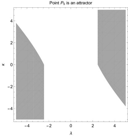
Figure 1: Region space of the free parameters $\left\{\lambda,\kappa\right\}$ in which point $P_{5}$ is an attractor.

$P_{6}=\left(-\frac{\lambda}{\sqrt{6}},\sqrt{1-\frac{\lambda^{2}}{6}},1\right)$ with physical properties similar to $P_{5}$. The eigenvalues of the linearized system are $e_{1}\left(P_{6}\right)=\lambda^{2}~{},~{}e_{2}\left(P_{6}\right)=\frac{1}{2}\left(\lambda^{2}-6\right),~{}e_{3}\left(P_{6}\right)=-\left(6-\kappa\lambda-\lambda^{2}\right)$ from where we infer that $P_{6}$ can not be a stable point while it is a saddle point for $\lambda^{2}<6$ or $\left\{\lambda<0,\kappa<\frac{6-\lambda^{2}}{\lambda}\right\}$ or $\left\{\lambda>0,\kappa>\frac{6-\lambda^{2}}{\lambda}\right\}$.

$P_{7}=\left(\frac{\sqrt{6}}{\kappa+\lambda},\sqrt{\frac{\kappa}{\kappa+\lambda}},-1\right)$  describes the so-called hyperinflation exact solution in which both the scalar fields contribute to the cosmological fluid. The equation of state parameter is $w_{eff}\left(P_{7}\right)=1-\frac{2\kappa}{\kappa+\lambda}$ which means $w_{eff}\left(P_{7}\right)<-\frac{1}{3}$ for $\ \left\{\lambda<0~{}|~{}\kappa>-\lambda\text{ or }\kappa<2\lambda\right\}$ or $\left\{\lambda>0~{}|~{}\kappa<-\lambda\text{ or }\kappa>2\lambda\right\}$. The asymptotic solution describes an inflationary universe. Moreover, it is important to mention that the point is physically acceptable when $\frac{\kappa}{\kappa+\lambda}>0~{}$and exist when $\kappa+\lambda\neq 0$. The eigenvalues of the linearized system are $e_{1}\left(P_{7}\right)=-\frac{6\lambda}{\kappa+\lambda}~{},~{}e_{2}\left(P_{7}\right)=\frac{3\kappa}{\kappa+\lambda}+\frac{\sqrt{3\kappa}}{\kappa+\lambda}\left(27\kappa-4\left(\kappa^{2}-6\right)\lambda-8\kappa\lambda^{2}-4\lambda^{3}\right)^{\frac{1}{2}}$,  $e_{3}\left(P_{7}\right)=\frac{3\kappa}{\kappa+\lambda}-\frac{\sqrt{3\kappa}}{\kappa+\lambda}\left(27\kappa-4\left(\kappa^{2}-6\right)\lambda-8\kappa\lambda^{2}-4\lambda^{3}\right)^{\frac{1}{2}}$. The region space of the variables $\left\{\lambda,\kappa\right\}$ in which point $P_{7}$ is an attractor is presented in Fig. 2.

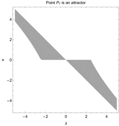
Figure 2: Region space of the free parameters $\left\{\lambda,\kappa\right\}$ in which point $P_{7}$ is an attractor.

$P_{8}=\left(-\frac{\sqrt{6}}{\kappa+\lambda},\sqrt{\frac{\kappa}{\kappa+\lambda}},1\right)$ has physical properties similar to point $P_{7}$. The eigenvalues of the linearized system are $e_{1}\left(P_{8}\right)=\frac{6\lambda}{\kappa+\lambda}~{},~{}e_{2}\left(P_{7}\right)=-\frac{3\kappa}{\kappa+\lambda}+\frac{\sqrt{3\kappa}}{\kappa+\lambda}\left(27\kappa-4\left(\kappa^{2}-6\right)\lambda-8\kappa\lambda^{2}-4\lambda^{3}\right)^{\frac{1}{2}}$,  $e_{3}\left(P_{7}\right)=-\frac{3\kappa}{\kappa+\lambda}-\frac{\sqrt{3\kappa}}{\kappa+\lambda}\left(27\kappa-4\left(\kappa^{2}-6\right)\lambda-8\kappa\lambda^{2}-4\lambda^{3}\right)^{\frac{1}{2}}$. Then, it follows that $P_{7}$ is a saddle point.

$P_{9}=\left(0,0,0\right)\,\ \$describes the Minkowski spacetime, where $H=0$. This point describes the transition where the Hubble function changes the sign. The eigenvalues of the linearized system are found to be zero $e_{1}\left(P_{9}\right)=0~{},~{}e_{2}\left(P_{9}\right)=0~{}$ and $e_{3}\left(P_{9}\right)=0$. By numerical inspection it is shown this point is always a saddle point.

Figs. 3 and 4 show two-dimensional phase space portraits for the dynamical system (14)-(16) for different values of the free parameters $\lambda,~{}\kappa$. In Figs. 3, orbits in the $x-y$ plane are displayed; in Fig. 4 orbits in the $x-\eta$ and $y-\eta$ planes are presented. In Figs. 5 orbits in the special case $\kappa+\lambda=0$ in a two-dimensional phase space are presented. Moreover, Fig. 6 shows orbits of the three-dimensional phase space of the dynamical system under study.

Figure 3: Two-dimensional phase space portrait for the dynamical system (14)-(16) in the $x-y$ plane for $\eta^{2}=1$ and $\eta=0$.

Figure 4: Two-dimensional phase space portrait for the dynamical system (14)-(16) in the $x-\eta$ and $y-\eta$ planes.

Figure 5: Two-dimensional phase space portrait for the dynamical system (14)-(16) in the $x-y$ plane for $\eta^{2}=1,~{}\eta=0$, and in the $x-\eta$ and $y-\eta$ planes, for $\kappa+\lambda=0$.

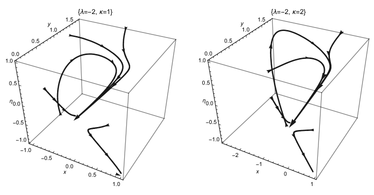
Figure 6: Trajectories in the three-dimensional phase space for the dynamical system (14)-(16) for different values of the free parameters $\lambda$ and $\kappa$.

III.2 Analysis at infinity

We continue our analysis by studying the existence of stationary points at the infinity. For this reason, we perform the change of variables by assuming the Poincaré variables

$$x=\frac{\rho}{\sqrt{1-\rho^{2}}}\cos\chi\cos\theta,~{}~{}y=\frac{\rho}{\sqrt{1-\rho^{2}}}\sin\chi\cos\theta~{},~{}\eta=~{}\frac{\rho}{\sqrt{1-\rho^{2}}}\sin\theta,$$ (20)

where $\chi\in[0,\pi],~{}\theta\in[-\frac{\pi}{2},\frac{\pi}{2}]$ and $0\leq\rho\leq 1$. Therefore, the dynamical system (14)-(16) reads

$$\frac{4}{\rho}\frac{d\rho}{d\sigma} =\sqrt{6}\kappa\left(\rho^{2}-1\right)\left(\cos\theta+\cos\left(3\theta\right)\right)\cos\chi+3\left(3\rho^{2}-2-\left(5\rho^{2}-2\right)\cos 2\theta\right)\sin\theta$$

$$+6\left(3\rho^{2}-2\right)\cos^{2}\theta\cos\left(2\chi\right)\sin\theta~{},~{}$$ (21)

$$\frac{d\chi}{d\sigma} =\frac{1}{4}\left(\sqrt{6}\left(\lambda+\left(2\kappa+\lambda\right)\cos\left(2\theta\right)\right)\frac{\sin\chi}{\cos\theta}+6\sin\theta\sin\left(2\chi\right)\right)~{},$$ (22)

$$\frac{d\theta}{d\sigma} =\frac{1}{2}\cos\left(2\theta\right)\left(\sqrt{6}\kappa\cos\chi\sin\theta+6\sin^{2}\chi\cos\theta\right)~{},$$ (23)

where the new independent variable $\sigma$ is defined as $d\sigma=\frac{\sqrt{1-\rho^{2}}}{\rho}d\tau$.

We work at the infinity in which $\rho\rightarrow 1^{+}$. As $\rho\rightarrow 1^{+}$ the leading terms in (21) are

$$\frac{d\rho}{d\sigma}=\frac{3}{4}\sin(\theta)\left(2\cos^{2}(\theta)\cos(2\chi)-3\cos(2\theta)+1\right).$$ (24)

Then, we analyze the stability at infinity using the asymptotic equation (24) together with equations (22) and (23). The radial equation (24) does not contain the radial coordinate, so the singular points can be obtained using the angular equations only. Setting $\chi^{\prime}(\sigma)=0$, and $\theta^{\prime}(\sigma)=0$, we obtain the singular points which are listed below. The stability of these points is studied by analyzing first the stability of the angular coordinates and then deducing, from the sign of equation (24), the stability on the radial direction. Note that from $\frac{d\rho}{d\sigma}=c$, if $c>0$ the $\rho$ increases and reaches the value one, while when $c<0$, $\rho$ decreases and goes far from the value $\rho=1$.

The stationary points of the two dimensional dynamical system (22), (23) in the range $\chi\in[0,\pi],~{}\theta\in[-\frac{\pi}{2},\frac{\pi}{2}]$ are:

$Q_{1}^{\pm}=\left(0,\pm\frac{\pi}{4}\right)$ that describe stiff fluid solutions, $w_{eff}\left(Q_{1}^{\pm}\right)=0$, with $\eta\neq 0$. The eigenvalues of the linearized system are $e_{1}\left(Q_{1}^{\pm}\right)=-\sqrt{3}\kappa~{},~{}e_{2}\left(Q_{2}^{\pm}\right)=\frac{1}{2}\left(\sqrt{3}\lambda\pm 3\sqrt{2}\right)$, while from (24) we find, $\frac{d\rho}{d\sigma}=\pm\frac{3}{2\sqrt{2}}$ as $\rho\rightarrow 1^{+}$, where we find point $Q_{1}^{+}$ is a sink when $\left\{\kappa>0,\lambda<-\sqrt{6}\right\}$ while $Q_{2}^{-}$ is always a source.

$Q_{2}=\left(0,0\right)$ is a stationary point where $\eta=0$, which means that $H=0$; hence, it changes the sign. The eigenvalues of the linearized system are $e_{1}\left(Q_{2}\right)=\sqrt{\frac{3}{2}}\kappa~{},~{}e_{2}\left(Q_{2}\right)=\sqrt{\frac{3}{2}}\left(\kappa+\lambda\right)$, while from (24) we have $\frac{d\rho}{d\sigma}=0$. Therefore, $e_{1}\left(Q_{2}\right)<0,~{}e_{2}\left(Q_{2}\right)<0$ when $\kappa<0$ and $\lambda<-\kappa$.

$Q_{3}^{\pm}=\left(\pi,\pm\frac{\pi}{4}\right)$ have physical properties similar to $Q_{1}^{\pm}$. The eigenvalues of the linearized system are $e_{1}\left(Q_{3}^{\pm}\right)=\sqrt{3}\kappa~{},~{}e_{2}\left(Q_{3}^{\pm}\right)=\frac{1}{2}\left(-\sqrt{3}\lambda\pm 3\sqrt{2}\right)$. From equation (24) it follows $\frac{d\rho}{d\sigma}=\pm\frac{3}{2\sqrt{2}}$ from where we conclude that $Q_{3}^{+}$ is a sink for $\kappa<0$ and $\lambda>\sqrt{6}$ while $Q_{3}^{-}$ is always a source.

$Q_{4}=\left(\pi,0\right)~{}$is a point in which $\eta=0$. The eigenvalues of the linearized system are $e_{1}\left(Q_{2}\right)=-\sqrt{\frac{3}{2}}\kappa~{},~{}e_{2}\left(Q_{2}\right)=-\sqrt{\frac{3}{2}}\left(\kappa+\lambda\right)$. Hence, they are negative when $\kappa>0,~{}\lambda>-\kappa$. Moreover, from (24) it follows $\frac{d\rho}{d\sigma}=0$.

$Q_{5}^{\pm}=\left(\pm\arccos\left(\frac{\lambda}{\sqrt{6}}\right),-\frac{\pi}{4}\right)$ describes a scaling solution with $w_{ff}\left(Q_{5}^{\pm}\right)=\frac{\lambda^{2}}{3}-1$, they are the analog of point $P_{5}$ at infinity. Equation (24) gives $\frac{d\rho}{d\sigma}=-\frac{\lambda^{2}}{4\sqrt{2}}$, while the eigenvalues of the linearized system are $e_{1}\left(Q_{5}^{\pm}\right)=\frac{1}{\sqrt{2}}\left(6-\lambda\left(\kappa+\lambda\right)\right),~{}e_{2}\left(Q_{5}^{\pm}\right)=\frac{1}{2\sqrt{2}}\left(6-\lambda^{2}\right)$. Therefore, we conclude that for $\left\{\lambda^{2}<0~{},~{}\kappa\lambda<6-\lambda^{2}\right\}$ the points are sources. Otherwise they are saddle points.

$Q_{6}^{\pm}=\left(\pm\arccos\left(-\frac{\lambda}{\sqrt{6}}\right),\frac{\pi}{4}\right)$  are the equivalent points of $P_{6}$ at infinity where we find $\frac{d\rho}{d\sigma}=\frac{\lambda^{2}}{4\sqrt{2}}$, $e_{1}\left(Q_{6}^{\pm}\right)=\frac{3}{2\sqrt{2}}\left(\lambda^{2}-2\right),e_{2}\left(Q_{6}^{\pm}\right)=\frac{\lambda^{2}-\kappa\lambda-6}{\sqrt{2}}$. Therefore, we infer that the points are sinks when $\lambda^{2}<2$ and $\kappa\lambda>\lambda^{2}-6$.

Furthermore, we find the stationary points  $Q_{7}^{\pm}=\left(\pm 2\arctan\left(\delta^{-}\right),2\arctan\left(\upsilon^{+}\right)\right),Q_{8}^{\pm}=\left(\pm 2\arctan\left(\delta^{+}\right),-2\arctan\left(\upsilon^{+}\right)\right)$ , $Q_{9}^{\pm}=\left(\pm 2\arctan\left(\delta^{-}\right),2\arctan\left(\upsilon^{-}\right)\right)$ and $Q_{10}^{\pm}=\left(\pm 2\arctan\left(\delta^{+}\right),-2\arctan\left(\upsilon^{-}\right)\right)$, where $\delta^{\pm}=\sqrt{\frac{12+\kappa\left(\kappa+\lambda\right)\pm 2\sqrt{6\left(6+\kappa\left(\kappa+\lambda\right)\right)}}{\left(\kappa+\lambda\right)}}~{}~{},~{}\upsilon^{\pm}=\frac{\sqrt{6+\kappa\left(\kappa+\lambda\right)}\pm\sqrt{6+\left(\kappa+\lambda\right)\left(2\kappa+\lambda\right)}}{\left(\kappa+\lambda\right)}$. The points are real when $\left\{\kappa<0,~{}\lambda>0\text{ and }\kappa+\lambda>0\right\}$ or $\left\{\kappa>0,~{}\lambda<0\text{ and }\kappa+\lambda<0\right\}$. The asymptotic solutions describe scaling solutions, with the same physics of point $P_{7}$. In Fig. 7 the regions of $\left(\lambda,\kappa\right)$ in which the points are sinks are present.

Figure 7: Region plot in the space of the free variables $\left(\lambda,\kappa\right)$ where the stationary points  $Q_{7}^{\pm},~{}$ $Q_{8}^{\pm}$,  $Q_{8}^{\pm}\$and  $Q_{10}^{\pm}$ are attractors.

Finally, in Fig. 8 we present phase-space portraits for the dynamical system (22), (23) for different values of the free parameters $\left(\lambda,\kappa\right).$ Hence, it is clear that the Minkowski universes described by points $Q_{2}$ and $Q_{4}$ are saddle points.

Figure 8: Phase-space portraits for the dynamical system (22), (23) for different values of the free parameters $\left(\lambda,\kappa\right)$

IV Evolution of the perturbations

Let us now study the evolution of the cosmological perturbations around the stationary points of special physical interests. In order to perform such analysis we select to apply the linear perturbation theory in the Newtonian gauge, where the perturbed spacetime around the spatially FLRW space is written as follows amebook

$$ds^{2}=a^{2}\left(\sigma\right)\left(-\left(1+2\Phi\left(\sigma,x,y,z\right)\right)d\sigma^{2}+\left(1-2\Phi\left(\sigma,x,y,z\right)\right)\left(dx^{2}+dy^{2}+dz^{2}\right)\right),$$ (25)

where $\sigma$ is the conformal time $\sigma=\int a^{-1}dt$. Function $\Phi\left(\sigma,x,y,z\right)$ includes the perturbation terms.  As far as the two scalar fields $\phi~{}$and $\psi$, are concerned, they are perturbed as $\phi+\delta\phi~{},~{}\psi+\delta\psi$ where we select $\varphi\left(\sigma,x,y,z\right)=\delta\phi$ and $\xi\left(\sigma,x,y,z\right)=\delta\psi$.

In the linear perturbation theory in the Newtonian gauge the perturbative components of Einstein’s tensor are

$$\delta G_{0}^{0} =-\frac{2}{a^{2}}\nabla^{2}\Phi+\frac{6}{a}\mathcal{H}\left(\dot{\Phi}+a\mathcal{H}\Phi\right)\,,$$ (26)

$$\delta G_{i}^{0} =-\frac{2}{a^{2}}\nabla_{i}\left(\dot{\Phi}+a\mathcal{H}\Phi\right)\,,$$ (27)

$$\delta G_{i}^{i} =2\Phi\left(\frac{2}{a}\mathcal{\dot{H}}+3\mathcal{H}^{2}\right)+\frac{2}{a^{2}}\left(\ddot{\Phi}+3a\mathcal{H}\dot{\Phi}\right)\,,$$ (28)

where now dot means derivative with respect the variable $\sigma$, and $\mathcal{H}=\frac{\dot{a}}{a^{2}}$ is the Hubble parameter in the new frame and $i,j,k=1,2,3$.

The contribution of the scalar fields in the linear perturbations $\delta T_{\mu\nu}$ is as follows

$$\delta T_{0}^{0}=-\frac{1}{a^{2}}\left(\dot{\phi}\dot{\varphi}-\dot{\phi}^{2}\Phi\right)-V_{,\phi}\varphi+\frac{e^{\kappa\phi}}{a^{2}}\left(\dot{\psi}\dot{\xi}-\dot{\psi}^{2}\Phi\right)+\frac{e^{\kappa\phi}}{2a^{2}}\varphi\dot{\psi}^{2}$$ (29)

$$\delta T_{i}^{\left(d\right)0}=\frac{1}{a^{2}}\nabla_{i}\left(\dot{\phi}\varphi-e^{\kappa\phi}\dot{\psi}\xi\right).$$ (30)

$$\delta T_{i}^{i}=\frac{1}{a^{2}}\left(\dot{\phi}\dot{\varphi}-\dot{\phi}^{2}\Phi\right)-V_{,\phi}\varphi-\frac{e^{\kappa\phi}}{a^{2}}\left(\dot{\psi}\dot{\xi}-\dot{\psi}^{2}\Phi\right)+\frac{e^{\kappa\phi}}{2a^{2}}\varphi\dot{\psi}^{2}$$ (31)

Furthermore, from the equation of motions (5), (6), that is, the conservation law $T_{~{}~{}~{};\nu}^{\mu\nu}=0$, we find for the following system which describes the solution of the perturbations

$$\frac{1}{a^{2}}\left(\ddot{\varphi}-\nabla^{2}\varphi-4\dot{\Phi}\dot{\phi}\right)+\frac{2}{a}\mathcal{H}\dot{\varphi}+\frac{\kappa^{2}}{2a^{2}}e^{\kappa\phi}\dot{\psi}^{2}\varphi+V_{,\phi\phi}\varphi+2\Phi V_{,\phi}=0,$$ (32)

$$\frac{1}{a^{2}}\left(\ddot{\xi}-\nabla^{2}\xi-4\dot{\Phi}\dot{\psi}\right)+\frac{2}{a}\mathcal{H}\dot{\xi}+\frac{\kappa}{a^{2}}\dot{\psi}\dot{\varphi}=0\,,$$ (33)

We define the new independent variable $\tau$ such that,

$$\frac{1}{a}\frac{d}{d\sigma} =\sqrt{1+\mathcal{H}^{2}}\frac{d}{d\ln a},$$ (34)

$$\frac{1}{a^{2}}\frac{d^{2}}{d\sigma^{2}} =\left(1+\mathcal{H}^{2}\right)\frac{d^{2}}{d\tau^{2}}+\mathcal{HH}^{\prime}$$ (35)

where a prime means total derivative with respect to $\tau$, i.e. $\mathcal{H}^{\prime}=\frac{d\mathcal{H}}{d\tau}$.

In the new variables, equations (32) and (33) become

$$\varphi^{\prime\prime}+\eta\left(\frac{1-3w_{eff}}{2}\right)\varphi^{\prime}-4\sqrt{6}\Phi^{\prime}x+\frac{k^{2}}{a^{2}\left(1+\mathcal{H}^{2}\right)}\varphi+3\kappa^{2}z^{2}\varphi+3\lambda y^{2}\left(\lambda\Gamma\left(\lambda\right)\varphi+2\Phi\right)=0$$ (36)

$$\xi^{\prime\prime}+\eta\left(\frac{1-3w_{eff}}{2}\right)\xi^{\prime}-4\sqrt{6}\Phi^{\prime}e^{-\frac{\kappa}{2}\phi}z+\frac{k^{2}}{a^{2}\left(1+\mathcal{H}^{2}\right)}\xi+\sqrt{6}\kappa\varphi ze^{-\frac{\kappa}{2}\phi}=0.$$ (37)

in which we replaced $\varphi=\varphi\left(\tau\right)e^{-ikx^{i}}$, $\xi=\xi\left(\tau\right)e^{-ikx^{i}}$ and $\Phi=\Phi\left(\tau\right)e^{-ikx^{i}}$ and we assumed $\eta=\frac{\mathcal{H}}{\sqrt{1+\mathcal{H}^{2}}},$ while we have replaced $\eta\frac{\mathcal{H}^{\prime}}{\mathcal{H}}=-\frac{3}{2}\left(1+w_{eff}\right)\,.$

In addition, from the field equations we find

$$\Phi^{\prime}=-\frac{\sqrt{6}}{2}\left(x\varphi-e^{\frac{\kappa}{2}\phi}z\xi\right)-\eta\Phi.$$ (38)

$$-\frac{2k^{2}}{a^{2}\sqrt{1+\mathcal{H}^{2}}}\Phi+6\left(\eta\Phi^{\prime}+\eta^{2}\Phi\right)=-\left(\sqrt{6}x\varphi^{\prime}-6x^{2}\Phi\right)-3\lambda y^{2}\varphi+\left(\sqrt{6}e^{\frac{\kappa}{2}\phi}z\xi^{\prime}-6z^{2}\Phi\right)+3\varphi z^{2}.$$ (39)

We proceed by doing the change of variables $\xi=\zeta e^{-\frac{\kappa}{2}\phi}$, thus equations (37), (38) and (39) are written as follows

$$0 =\zeta^{\prime\prime}-\frac{\sqrt{6}\kappa}{2}\zeta^{\prime}x+\frac{\kappa^{2}\sqrt{6}}{4}\zeta x^{\prime}+\frac{k^{2}}{a^{2}\left(1+\mathcal{H}^{2}\right)}\zeta-4\sqrt{6}\Phi^{\prime}z$$ (40)

$$+\left(\eta\left(\frac{1-3w_{eff}}{2}\right)\right)\left(\zeta^{\prime}-\frac{\sqrt{6}\kappa}{2}\zeta x\right)+\sqrt{6}\kappa\varphi z,$$

$$\Phi^{\prime}=-\frac{\sqrt{6}}{2}\left(x\varphi-z\zeta\right)-\eta\Phi,$$ (41)

and

$$0 =-\left(\sqrt{6}x\varphi^{\prime}-6x^{2}\Phi\right)-3\lambda y^{2}\varphi+\left(\sqrt{6}z\left(\zeta^{\prime}-\frac{\sqrt{6}\kappa}{2}\zeta x\right)-6z^{2}\Phi\right)$$ (42)

$$+3\varphi z^{2}+\frac{2k^{2}}{a^{2}\sqrt{1+\mathcal{H}^{2}}}\Phi-6\left(\eta\Phi^{\prime}+\eta^{2}\Phi\right).$$

Until now we have considered variables at the finite regime. From the results of the previous section, we found that at the infinity the stationary points have the same physical properties as that of the finite regime. Hence, in order to study the evolution of the perturbations at the asymptotic solutions we select to work with the finite variables only.

IV.1 Perturbations at the stationary points $P_{7}$ and $P_{8}$

We carry on our analysis by studying the qualitative evolution for the perturbations on the background space in which the physical solution is described by the asymptotic solutions at the stationary points. We observe that equations (36), (41) and (42) are independent on $\zeta$ when the second field does not contribute in the background space, that is, for $z=0$, the evolution of the perturbations it is similar with that for the quintessence scalar field. Hence, we shall on the new stationary points which describe the hyperbolic inflation, points $P_{7}$ and $P_{8}$. For the exponential potential $\Gamma\left(\lambda\right)=1,$ while at the stationary points $P_{7}$ and $P_{8}$ we find $\eta^{2}=1$, which means that $\mathcal{H}^{2}\rightarrow+\infty.$

Consequently, the perturbation equations for the scalar fields read

$$0 =\varphi^{\prime\prime}+\frac{(1-3w_{eff})}{2}\eta\varphi^{\prime}+3\kappa^{2}z^{2}\varphi$$

$$+\frac{\lambda y^{2}\left(-3\varphi\left((\lambda+1)z^{2}-\lambda\left(x^{2}+y^{2}\right)\right)+\sqrt{6}\left(x\varphi^{\prime}-z\zeta^{\prime}\right)+3\kappa xz\zeta\right)}{x^{2}-z^{2}}+$$

$$+\frac{2\left(\varphi\left(6x^{3}-6xz^{2}+\sqrt{6}\eta\left(\lambda y^{2}-z^{2}\right)\right)+\zeta\left(-6x^{2}z+\sqrt{6}\eta\kappa xz+6z^{3}\right)+2\eta x\varphi^{\prime}-2\eta z\zeta^{\prime}\right)}{x^{2}-z^{2}},$$ (43)

$$0 =\zeta^{\prime\prime}+\frac{(1-3w_{eff})}{2}\eta\left(\zeta^{\prime}-\frac{\sqrt{6}}{2}\kappa x\zeta\right)-\sqrt{\frac{3}{2}}\kappa x\zeta^{\prime}+2\sqrt{6}\kappa z\varphi+$$

$$-\frac{2z\left(\varphi\left(6x^{3}-6xz^{2}+\sqrt{6}\eta\left(\lambda y^{2}-z^{2}\right)\right)+z\zeta\left(-6x^{2}+\sqrt{6}\eta\kappa x+6z^{2}\right)+2\eta x\varphi^{\prime}-2\eta z\zeta^{\prime}\right)}{z^{2}-x^{2}}.$$ (44)

We write the two second-order differential equations as a linear system

$$\varphi^{\prime} =p_{\varphi}~{},~{}$$ (45)

$$\zeta^{\prime} =p_{\zeta}$$ (46)

$$p_{\varphi}^{\prime} =f\left(\varphi,\zeta,p_{\varphi},p_{\zeta}\right)$$ (47)

$$p_{\zeta}^{\prime} =g\left(\varphi,\zeta,p_{\varphi},p_{\zeta}\right)~{}$$ (48)

For the background solutions described by the stationary points $P_{7}$ and $P_{8}$, the dynamical system (45)-(48) admit the stationary point $\left(\varphi,\zeta,p_{\varphi},p_{\zeta}\right)=\left(0,0,0,0\right)$. The real part of the eigenvalues for the linear system are plot numerically. In Fig. 9 we plot the real part of the eigenvalues for the system (45)-(48) at the point $P_{7}$, while in Fig. 10 we plot the eigenvalues for the background solution described by $P_{8}$.

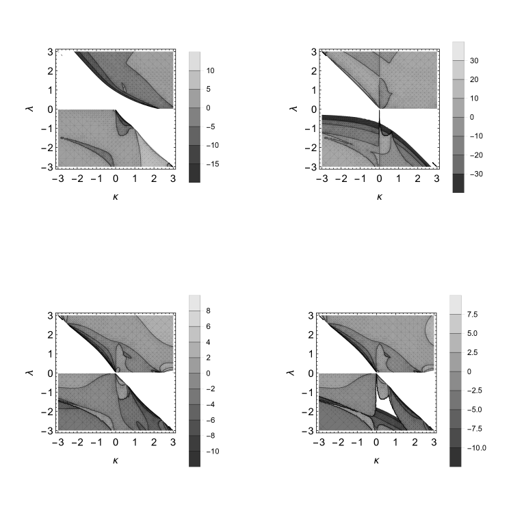
Figure 9: Contour plots for the real part for the four eigenvalues of the linear system (45)-(48) in the space of the free variables $\left\{\kappa,\lambda\right\}$ with background solution described by $P_{7}$.

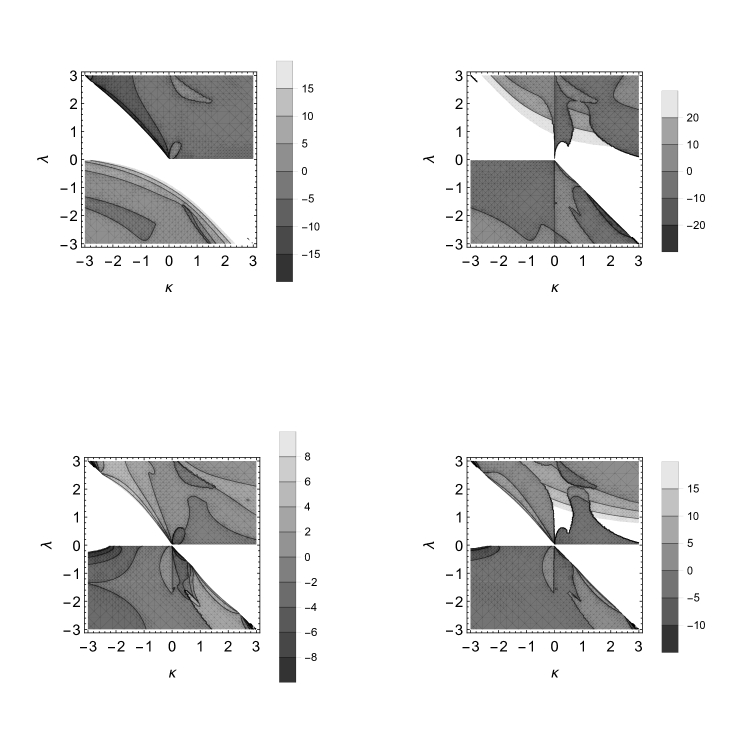
Figure 10: Contour plots for the real part for the four eigenvalues of the linear system (45)-(48) in the space of the free variables $\left\{\kappa,\lambda\right\}$ with background solution described by $P_{8}$.

The equation of state parameter for the background solution at the stationary points $P_{7}$ and $P_{8}$ is $w_{eff}=1-\frac{2\kappa}{\kappa+\lambda}$. Thus for $\kappa=\lambda$, $w_{eff}=0$ which means that the solution describes the matter era. The real part for the eigenvalues of the perturbation system in the matter solution with $\kappa=\lambda$ is presented in Fig. 11. We observe that not all the eigenvalues are negative which means that the perturbations do not decay.

Figure 11: Real part for the four eigenvalues of the linear system (45)-(48) in in the case where $P_{7}$ and $P_{8}$ describe the matter era.

V Conclusions

In this work, we have investigated the global dynamics of a multiscalar field cosmological model known as hyperbolic Chiral-Phantom theory. It is a two-scalar field theory in which the scalar fields are minimally coupled to gravity, but they interact in the kinetic part. In particular, the kinetic Lagrangian for the scalar fields defines a two-dimensional manifold of constant negative curvature, i.e., a hyperbolic plane. Moreover, one of the two scalar fields is assumed to have a negative kinetic term, which means that its energy density can be negative and have phantom properties. This model has been recently proposed in and3 and it was found that provides a different cosmological history from the standard hyperbolic Chiral theory. While there are similarities with the quintom theory, the two theories are dissimilar.

To study the cosmological history provided by this model, we use new dimensionless variables different from the usual $H$-normalization because the Hubble function can change the sign and vanishes, so, the $H$-normalization is not applicable. In terms of the new variables, the field equations were written in the equivalent form of an algebraic-differential system. For this system, we have investigated the stationary points and their stability. Each stationary point describes a specific epoch in the cosmological evolution. The stationary points were investigated in the local variables, also at the infinity region with the use of Poincaré variables. Furthermore, for the scalar field potential, we have considered the exponential potential.

In the finite regime with the use of local variables, we found that the dynamical system admits nine stationary points. That is a greater number from that of the quintessence model, and of the standard hyperbolic model. Points $P_{1},~{}P_{2}$, $P_{3}$, $P_{4}$ and $P_{5},~{}P_{6}$ can be categorized as $\left\{P_{1},P_{3}\right\},~{}\left\{P_{2},P_{4}\right\}~{}$and $\left\{P_{5},P_{6}\right\}$. These three categories describe the three stationary points of the quintessence scalar field model with exponential potential cop1 . The two first categories describe the stiff fluid solutions, while the third category describes the scaling solution. Moreover, from the stability analysis of the stationary points, we found that the quintessence model is possible to be an attractor for the system. Stationary points $P_{7},~{}P_{8}$ describe the so-called hyperbolic inflation, while $P_{9}$ corresponds to Einstein’s universe in the spatially flat FLRW background space, that is, the Minkowski space. Point $P_{9}$ was found to be a saddle point. $P_{7}$ can be an attractor while $P_{8}$ is a saddle point.

However, by using the Poincaré variables we were able to find new stationary points. Specifically, we found ten families of stationary points. Points $\left\{Q_{1}^{\pm},Q_{3}^{\pm},Q_{5}^{\pm},Q_{6}^{\pm}\right\}$ describe the limit of quintessence theory, point $\left\{Q_{2},Q_{4}\right\}$ describe the Einstein static space; while the stationary points $\left\{Q_{7}^{\pm},Q_{8}^{\pm},Q_{9}^{\pm},Q_{10}^{\pm}\right\}$ describe the hyperbolic inflation similarly to the points $P_{7}$ and $P_{8}$.

Furthermore, we investigated the linear cosmological perturbations in the Newtonian gauge. We derived the perturbed field equations and the equations of motions for the evolution of the perturbation terms for the scalar fields. The stability properties for the scalar field perturbations were investigated at the background solutions where the two scalar fields contribute to the cosmological fluid.

The theory provides a rich cosmological history, either in the finite or the infinity regime. That is an important property because there is more than one set of initial conditions which can be the same cosmological evolution. Furthermore, this model can play a role not only in the description of inflation, as it is mainly used, but also can be a dark energy candidate. In future work, we plan to investigate further considerations by using cosmological observations.

- (1) A.A. Starobinsky, Phys. Lett. B 91, 99 (1980)
- (2) A. Guth, Phys. Rev. D 23, 347 (1981)
- (3) V. Muller, H.-J. Schmidt and A.A. Starobinsky, Phys. Lett. B 202, 2, 198 (1988)
- (4) L.A Kofman, A.D. Linde and A.A. Starobinsky, Phys. Lett. B 157, 5-6, 361 (1985)
- (5) D. Wands, Lect. Notes Phys. 738, 275 (2008)
- (6) D.I. Kaiser, E.A. Mazenc and E.I. Sfakianakis, Phys. Rev. D 87, 064004 (2013)
- (7) D. Langlois and S. Renaux-Peterl, JCAP 0804, 017 (2008)
- (8) K.Y. Choi, S.A. Kim and B. Kyae, Nucl. Phys. B 861, 271 (2021)
- (9) D.H. Lyth, JCAP 0511, 006 (2005)
- (10) O. Bertolami, P. Carrilho and J. Páramos, Phys. Rev. D 86, 103522 (2012)
- (11) M. Cicoli, G. Dibitetto and F.G. Pedro, JHEP 2020, 35 (2020)
- (12) Y. Akrami, M. Sasaki, A.R. Solomon and V. Vardanyan, Multi-field dark energy: cosmic acceleration on a steep potential, [arXiv:2008.13660]
- (13) K.J. Ludwick, Mod. Phys. Lett. A 32, 28 (2017)
- (14) Y.-F. Cai, E.N. Saridakis, M.R. Setare and J.-Q. Xia, Phys. Rept. 493, 1 (2010)
- (15) S. Mishra and S. Chakraborty, EPJC 78, 917 (2018)
- (16) M.R. Setare and E.N. Saridakis, Phys. Rev. D 79, 043005 (2009)
- (17) E. Di Valentino, O. Mena, S. Pan, L. Visinelli, W. Yang, A. Melchiorri, D.F. Mota, A.G. Riess and J. Silk, In the Realm of the Hubble tension - a Review of Solutions, [arXiv:2103.01183]
- (18) S.V. Chervon, Quantum Matter 2, 71 (2013)
- (19) I.V. Fomin, J. Phys.: Conf. Ser. 918, 012009 (2017)
- (20) S. V. Ketov, Quantum Non-linear Sigma Models, Springer-Verlag, Berlin, (2000)
- (21) A. R. Brown, Phys. Rev. Lett. 121, 251601 (2018)
- (22) S. Mizuno and S. Mukohyama, Phys. Rev. D 96, 103533 (2017)
- (23) P. Christodoulidis, D. Roest and E.I. Sfakianakis, JCAP 1911, 002 (2019)
- (24) A. Paliathanasis, Class. Quantum Grav. 37, 195014 (2020)
- (25) A. Paliathanasis and M. Tsamparlis, Phys. Rev. D 90, 043529 (2014)
- (26) A. Paliathanasis, G. Leon and S. Pan, Gen. Rel. Grav. 51, 106 (2019)
- (27) P. Christodoulidis, Probing the inflationary evolution using analytical solutions, [arXiv:1811.06456]
- (28) J. Socorro, S. Pérez-Payán, A. Espinoza-García and L.R. Díaz-Barrón, Anisotropic chiral cosmology: exact solutions (2021) [arXiv:2101.05973]
- (29) J. Socorro, S. Pérez-Payán, R. Hernández, A. Espinoza-García and L.R. Díaz-Barrón, Classical and quantum exact solutions for a FRW in chiral like cosmology (2020) [arXiv:2012.11108]
- (30) A. Giacomini, E. Gonzalez, G. Leon and A. Paliathanasis, Variational symmetries and superintegrability in multifield cosmology, (2021) [arXiv:2104.13649]
- (31) A. Paliathanasis and G. Leon, EPJC 80, 1099 (2020)
- (32) P. Christodoulidis and A. Paliathanasis, -field cosmology in hyperbolic field space: stability and general solutions, to appear in JCAP [arXiv:2101.09582]
- (33) S.D. Maharaj, A. Beesham, S.V. Chernov and A.S. Kubasov, Gravitation and Cosmology 23, 375 (2017)
- (34) N. Dimakis and A. Paliathanasis, Class. Quantum Grav. 38, 075016 (2021)
- (35) A. Paliathanasis and G. Leon, Class. Quantum Grav. 38, 075013 (2021)
- (36) E.J. Copeland, M. Sami and S. Tsujikawa, IJMPD 15, 1753 (2006)
- (37) A. Giacomini, S. Jamal, G. Leon, A. Paliathanasis and J. Saveedra, Phys. Rev. D 95, 124060 (2017)
- (38) A.A. Coley, Phys. Rev. D 62, 023517 (2000)
- (39) R. Lazkoz and G. Leon, Phys. Lett. B 638, 303 (2006)
- (40) A. Collinucci, M. Nielsen and T. Van Riet, Class. Quantum Grav. 22, 1269 (2005)
- (41) A.A. Coley and R.J. van den Hoogen, Phys. Rev. D 62, 023517 (2000)
- (42) L. Amendola and S. Tsujikawa, Dark Energy: Theory and Observations, Cambridge University Press, New York (2010)