A reverse quantitative isoperimetric type inequality for the Dirichlet Laplacian

Abstract.

A stability result in terms of the perimeter is obtained for the first Dirichlet eigenvalue of the Laplacian operator. In particular, we prove that, once we fix the dimension $n\geq 2$, there exists a constant $c>0$, depending only on $n$, such that, for every $\Omega\subset\mathbb{R}^{n}$ open, bounded and convex set with volume equal to the volume of a ball $B$ with radius $1$, it holds

$$\lambda_{1}(\Omega)-\lambda_{1}(B)\geq c\left(P(\Omega)-P(B)\right)^{2},$$

where by $\lambda_{1}(\cdot)$ we denote the first Dirichlet eigenvalue of a set and by $P(\cdot)$ its perimeter. The hearth of the present paper is a sharp estimate of the Fraenkel asymmetry in terms of the perimeter.

MSC 2020: 35J05, 35J57, 52A27
Keywords: Dirichlet-Laplace eigenvalue, Fraenkel asymmetry, Hausdorff asymmetry, quantitative inequality.

A REVERSE QUANTITATIVE ISOPERIMETRIC INEQUALITY

1. Introduction

Let $\Omega\subset\mathbb{R}^{n}$, with $n\geq 2$, be an open set with finite Lebesgue measure. The first Dirichlet-Laplacian eigenvalue associated to $\Omega$, that we denote by $\lambda_{1}(\Omega)$, is the least positive $\lambda$ such that

$$\begin{cases}-\Delta u=\lambda u&\mbox{in }\Omega\\ u=0&\mbox{on }\partial\Omega\end{cases}$$

admits non-trivial solutions in $H^{1}_{0}(\Omega)$. The classical result of Faber and Krahn states that, among measurable domains with fixed measure, $\lambda_{1}(\cdot)$ is minimized by a ball (see [10, 20, 26]). In other words, the following scaling invariant inequality holds:

$$\lambda_{1}(\Omega)|\Omega|^{2/n}\geq\lambda_{1}(B_{R})|B_{R}|^{2/n},$$ (1.1)

where by $|\Omega|$ we denote the volume of a measurable set $\Omega$, i.e. its Lebesgue measure, and by $B_{R}$ a geniric ball in $\mathbb{R}^{n}$ of radius $R$. Equality in (1.1) holds if and only if $\Omega$ is equivalent to a ball. Moreover, the quantity $\lambda_{1}(\Omega)$ can be variationaly characterized by

$$\lambda_{1}(\Omega)=\min_{\begin{subarray}{c}v\in H^{1}_{0}(\Omega)\\ v\nequiv 0\end{subarray}}\dfrac{\displaystyle\int_{\Omega}|Dv|^{2}\;dx}{\displaystyle\int_{\Omega}v^{2}\;dx}$$

and has the following scaling property, for every $t>0$,

$$\lambda_{1}(t^{2}\Omega)=t^{-2}\lambda_{1}(\Omega).$$

We refer to [21] and [19] as survay books on the argument.

In this paper we consider the following class of admissible sets

$$\mathcal{C}_{n}:=\{\Omega\subseteq\mathbb{R}^{n}\;|\;\Omega\text{ convex},\;|\Omega|=|B|\},$$

where $B$ is a ball of $\mathbb{R}^{n}$ with radius equal to $1$. From now on, we denote by $P(\Omega)$ the perimeter of $\Omega$ in the De Giorgi sense and by $\omega_{n}$ the volume of the ball $B$. Our starting point is the following conjecture in the planar case, that is stated in [11].

Conjecture 1.1.

[11] Let $\Omega$ be an open, bounded and convex subset of $\mathbb{R}^{2}$ with $|\Omega|=\omega_{n}$, then

$$\lambda_{1}(\Omega)-\lambda_{1}(B)\geq\beta\left(P(\Omega)-P(B)\right)^{3/2},$$ (1.2)

where $\beta:=\frac{4\cdot 3^{3/2}\;\zeta(3)}{\pi^{9/2}}$ and $\zeta(n)=\sum_{k=1}^{\infty}k^{-n}$ is the Riemann zeta function.

This conjecture is supported by numerical and analytical results, in particular we refer to [17, 16, 24].

Proposition 1.2.

[17] Let $\mathcal{P}^{*}_{k}$ be the regular polygon with $k$ edges and area equal to $\pi$. Then, as $k$ goes to $+\infty$,

$$\lambda_{1}(\mathcal{P}^{*}_{k})-\lambda_{1}(B)\sim\beta\left(P(\mathcal{P}_{k}^{*})-P(B)\right)^{3/2},$$

where $\beta$ is the constant defined in Conjecture 1.1.

The method used by Grinfeld and Strang in [17, 16] to prove this fact comes from differential geometry and relays on the calculus of moving surfaces. This result was also proved by Molinari in [24], using the Schwartz-Christoffel mappings, that are useful tools to express the Dirichlet eigenvalue of a polygon as a series expansion, relating each expansion term to a summation over Bessel functions.

By the way, we recall that the fundamental tone of the Dirichlet-Laplacian on polygons has been widely investigated and, nevertheless, many questions are still unsolved. The famous Polyá-Szegö conjecture [26],for example, states that among all the $k$-gons of given area the regular one achieves the least possible $\lambda_{1}$ and has been settled only for $k=3$ and $k=4$, that are the only cases for which it is possible to use the Steiner symmetrization (see [21, 26]).

Conjecture 1.1 is also supported by numerical observations, linked to the plot of the Blaschke-Santaló diagram for the triplet $(P(\cdot),\,\lambda_{1}(\cdot),\,|\cdot|\;)$, that is the sets of points

$$\{\left(P(\Omega),\lambda_{1}(\Omega)\right)\;|\;\;\Omega\in\mathcal{C}_{2}\}.$$

For these numerical results we refer to [1, 11]. In particular, in [11], the authors, by generating random polygons woth sides between $3$ and $30$, find out that regular polygons lay on the lower part of the diagram, while the shapes that lay on the upper part of the boundary of the diagram are smooth, expecting that stadii are a good approximation of the upper part.

In this work we are not able to prove Conjecture 1.1 in the plane. Instead, we prove a less strong result, but in every dimension. The main Theorem is the following.

Theorem 1.3.

Let $n\geq 2$. There exists a constant $c>0$, depending only on $n$, such that, for every $\Omega\in\mathcal{C}_{n}$, it holds

$$\lambda_{1}(\Omega)-\lambda_{1}(B)\geq c\left(P(\Omega)-P(B)\right)^{2},$$ (1.3)

being $B$ a ball of $\mathbb{R}^{n}$ with radius equal to $1$.

In order to obtain this, we prove an intermediate result, that is the core of this work and that has its own interest: there exists a constant $C>0$, depending only on the dimension $n$, such that, for every $\Omega\in\mathcal{C}_{n}$, it holds

$$\mathcal{A}_{F}(\Omega)\geq C\left(P(\Omega)-P(B)\right),$$ (1.4)

where $\mathcal{A}_{F}(\Omega)$ is the Fraenkel asymmetry of $\Omega$ (a $L^{1}-$distance between sets), defined as

$$\mathcal{A}_{F}(\Omega)=\min_{x\in\mathbb{R}^{n}}\bigg{\{}\dfrac{|\Omega\Delta B_{R}(x)|}{|\Omega|}\;:\>\text{$B_{R}(x)$ is a ball s.t. $|B_{R}(x)|=|\Omega|$}\bigg{\}},$$ (1.5)

denoting by $\Delta$ the symmetric difference between two sets and by $B_{R}(x)$ the ball of radius $R$ centered at the point $x$. Inequality (1.4) is true provided that the isoperimetric deficit $P(\Omega)-P(B)$ is small enough.

We prove (1.3) combing (1.4) with the sharp stability result for the Faber-Krahn inequality, proved in [6], that states that there exists a constant $\bar{C}>0$ such that for every open set $\Omega$ with $|\Omega|=\omega_{n}$, the following inequality holds:

$$\lambda_{1}(\Omega)-\lambda_{1}(B)\geq\bar{C}\mathcal{A}_{F}(\Omega)^{2}.$$ (1.6)

Unfortunately, as we will show providing a class of counter-examples, inequality (1.4) is not true when the difference of perimeters has exponent $3/4$, that is the target power to obtain (1.2), if we combine it with (1.6). The exponent $1$ of the difference of the perimeters in (1.4) is, indeed, an optimal exponent, since it is reached asymptotically by regular polygons with number of sides that goes to infinity. This is the reason for which we cannot use this strategy to prove Conjecture 1.1. So, this work represents a step forward to the resolution of this still open problem, generalising and obtaining some results also in dimension greater than $2$.

Moreover, we can say that inequality (1.4) is a sort of reverse quantitative inequality. We recall indeed that the sharp quantitative isoperimetric inequality, proved in [14] in any dimension, asserts that there exists a constant $K>0$ such that, for every Borel set $\Omega\subset\mathbb{R}^{n}$ with $|\Omega|=\omega_{n}$,

$$\left(P(\Omega)-P(B)\right)\geq K\mathcal{A}_{F}^{2}(\Omega).$$ (1.7)

On the contrary to (1.7), in our inequality (1.3) the terms of the difference of the perimeter is used as an asymmetry functional and, so, it is situated in the left hand side of the inequality, obtaining, in this way, a quantitative isoperimetric inequality for $\lambda_{1}(\cdot)$ in terms of the difference of the perimeter.

As a consequence of the fact that the Fraenkel asymmetry is a bounded quantity, more precicelly $\mathcal{A}_{F}(\Omega)\in[0,2)$ and is zero if and only if $\Omega$ is a ball, inequality (1.4) cannot be true when $\Omega$ is, for example, a long and flat domain and this is the reason for which, in the non local case, the proof of inequality (1.3) will be treated separatelly.

The paper is organized as follows. In Section $2$ we recall some preliminary definitions and results about convex sets and some spectral inequalities, proving also a lower bound of the Hausdorff distance in terms of the perimeter. Section $3$ is devoted to the proof of the sharp geometric inequality (1.4), that is the core of the present paper. Finally, in Section $4$ we prove the main Theorem 1.3.

2. Notations and preliminary results

2.1. Notations and basic definitions

We will use the following notations: $\cdot$ is the Euclidean scalar product in $\mathbb{R}^{n}$, $B$ is a generic ball of radius equal to $1$, $B(O)$ is the ball with radius equal to $1$ centered at the fixed origin $O=(0,\dots,0)$ and $\mathbb{S}^{n-1}$ is the unit sphere in $\mathbb{R}^{n}$. Moreover, we denote by $|\cdot|$ the Lebesgue measure of a set and by $\mathcal{H}^{k}$, for $k\in[0,n)$, the $k-$dimensional Hausdorff measure in $\mathbb{R}^{n}$. The perimeter of $\Omega$ in $\mathbb{R}^{n}$ will be denoted by $P(\Omega)$ and, if $P(\Omega)<\infty$, we say that $\Omega$ is a set of finite perimeter. In our case $\Omega$ is a convex and bounded set and this ensures us that it is a set of finite perimeter and that $P(\Omega)=\mathcal{H}^{n-1}(\partial\Omega)$.

For simplicity, we introduce the following notation:

$$\Delta\lambda_{1}(\Omega):=\lambda_{1}(\Omega)-\lambda_{1}(B),\qquad\Delta P(\Omega):=P(\Omega)-P(B).$$

We give the definition of tangential gradient, that can be found in [2].

Definition 2.1.

Let $\Omega$ be an open, bounded subset of $\mathbb{R}^{n}$ with Lipschitz boundary and let $u:\mathbb{R}^{n}\rightarrow\mathbb{R}$ be a Lipschitz function. We can define the tangential gradient of $u$ for almost every $x\in\partial\Omega$ as

$$\nabla_{\tau}u(x)=\nabla u(x)-\langle\nabla u(x),\nu_{\partial\Omega}(x)\rangle\nu_{\partial\Omega}(x),$$

where $\nu_{\partial\Omega}$ is the outer unit normal to $\partial\Omega$, whenever $\nabla u$ exists at $x$.

From now on we will consider open, bounded and convex subsets of $\mathbb{R}^{n}$, with $n\geq 2$. and, for the content of the following, we refer mainly to [27]. We start by recalling the definition of Hausdorff distance between two open, bounded and convex sets $\Omega,K\subset\mathbb{R}^{n}$, that is:

$$d_{\mathcal{H}}(\Omega,K)=\inf\left\{\varepsilon>0\;:\;\Omega\subset K+B_{\varepsilon},\;K\subset\Omega+B_{\varepsilon}\right\},$$ (2.1)

where by $+$ we denote the Minkowski sum between sets and $B_{\varepsilon}$ is a geniric ball of radius $\varepsilon$. Note that we have $d_{\mathcal{H}}(\Omega,K)=d_{\mathcal{H}}(\partial\Omega,\partial K)$ and that the following rescaling property holds

$$d_{\mathcal{H}}(t\Omega,tK)=t\,d_{\mathcal{H}}(\Omega,K),\quad t>0.$$

We recall the definition of support function of a convex set.

Definition 2.2.

Let $\Omega$ be an open, bounded and convex set of $\mathbb{R}^{n}$. The support function associated to $\Omega$ is defined, for every $y\in\mathbb{R}^{n}$, as follows:

$$h_{\Omega}(y)=\max_{x\in\Omega}\left(x\cdot y\right).$$ (2.2)

If there is no possibility of confusion, we use the notation $h$ instead of $h_{\Omega}$. It is easy to see that the support function associated to a ball of radius $R$ centered at the origin is constantly equal to $R$. In the following remark the relation between the Haussdorf distance and the support function is pointed out.

Remark 2.3.

Let $K,\Omega$ be two open, bounded and convex subsets of $\mathbb{R}^{n}$. It holds:

$$d_{\mathcal{H}}(\Omega,K)=||h_{\Omega}-h_{K}||_{L^{\infty}(\mathbb{S}^{n-1})}.$$

We define now another kind asymmetry, usually used for convex sets, different from the one recalled in (1.5).

Definition 2.4.

Let $\Omega$ be an open, bounded and convex subset of $\mathbb{R}^{n}$. We define the Hausdorff asymmetry as

$$\mathcal{A_{\mathcal{H}}}(\Omega)=\min_{x\in\mathbb{R}^{n}}\bigg{\{}\frac{d_{\mathcal{H}}(\Omega,B_{R}(x))}{R}\;:\>\text{$B_{R}(x)$ is a ball centered at $x$ s.t. $|B_{R}(x)|=|\Omega|$}\bigg{\}}.$$ (2.3)

Finally, if $\Omega\in\mathcal{C}_{n}$ is such that the origin $O\in\Omega$, then its boundary can be parametrized as :

$$\partial\Omega=\{y\in\mathbb{R}^{n}\;|\;y=r(x);\;x\in\mathbb{S}^{n-1}\}$$ (2.4)

and we have the following results (see for the exact computations [12]):

$$\mathcal{A}_{F}(\Omega)=\frac{1}{n}\displaystyle\int_{\mathbb{S}^{n-1}}|r^{n}(x)-1|\;d\mathcal{H}^{n-1}(x)$$ (2.5)

and

$$P(\Omega)=\int_{\mathbb{S}^{n-1}}\sqrt{r^{2(n-1)}(x)+r^{2(n-2)}(x)|\nabla_{\tau}r|^{2}}\>d\mathcal{H}^{n-1}.$$ (2.6)

In particular, if $\Omega\in\mathcal{C}_{2}$, we can use the classical polar coordinates representation, that this

$$\Omega=\bigg{\{}(r,\theta)\in[0,\infty)\times[0,2\pi)\;|\;r<\frac{1}{u(\theta)}\bigg{\}},$$ (2.7)

where $u$ is a positive and $2\pi-$periodic function, often called the gauge function of $\Omega$, for a reference see e.g [27, 18]. It is well known that $\Omega$ is convex if and only if $u^{\prime\prime}+u\geq 0$. Moreover, we can write the volume, the perimeter and the Fraenkel asymmetry of $\Omega$ in terms of $u$:

$$|\Omega|=\frac{1}{2}\displaystyle\int_{0}^{2\pi}\dfrac{1}{u^{2}(\theta)}\;d\theta;$$ (2.8)

$$P(\Omega)=\displaystyle\int_{0}^{2\pi}\dfrac{\sqrt{u^{2}+u^{\prime 2}}}{u^{2}}d\theta$$ (2.9)

and, setting $r(\theta):=1/u(\theta)$, we have

$$\mathcal{A}_{F}(\Omega)=\displaystyle\int_{0}^{2\pi}\big{|}\displaystyle\int_{r(\theta)}^{1}r\;dr|\;d\theta=\displaystyle\int_{0}^{2\pi}\dfrac{|1-r^{2}(\theta)|}{2}d\theta=\frac{1}{2}\displaystyle\int_{0}^{2\pi}\dfrac{|1-u^{2}(\theta)|}{u^{2}(\theta)}\;d\theta.$$ (2.10)

2.2. Definition and some properties on quermassintegrals

We give in this Section the definition of quermassintegrals, referring to [27]. Let $\Omega$ be an open, bounded and convex subset of $\mathbb{R}^{n}$. We define the outer parallel body of $\Omega$ at distance $\rho$ as the Minkowski sum

$$\Omega+\rho B=\{x+\rho y\in\mathbb{R}^{n}\;|\;x\in\Omega,\;y\in B\}.$$

The Steiner formula asserts that

$$|\Omega+\rho B|=\sum_{i=0}^{n}\binom{n}{i}W_{i}(\Omega)\rho^{i}.$$ (2.11)

and

$$P(\Omega+\rho B)=n\sum_{i=0}^{n-1}\binom{n}{i}W_{i+1}(\Omega)\rho^{i},$$ (2.12)

where the coefficients $W_{i}(\Omega)$ are known as quermassintegrals. In particular, we have:

$$W_{0}(\Omega)=|\Omega|;\qquad nW_{1}(\Omega)=P(\Omega);\qquad W_{n}(\Omega)=\omega_{n}$$ (2.13)

and

$$W_{n-1}(\Omega)=\dfrac{\omega_{n}}{2}\>\omega(\Omega),$$ (2.14)

where $\omega(\Omega)$ is called mean width of the convex body $\Omega$ and it is defined as

$$\omega(\Omega)=\frac{1}{n\omega_{n}}\int_{\mathbb{S}^{n-1}}\left(h_{\Omega}(x)+h_{\Omega}(-x)\right)\;d\mathcal{H}^{n-1}(x),$$ (2.15)

representing the mean value over all possible directions of the distance between parallel supporting hyperplanes to $\Omega$. Finally, we recall the Aleksandrov-Fenchel inequalities:

$$\left(\dfrac{W_{j}(\Omega)}{\omega_{n}}\right)^{\frac{1}{n-j}}\geq\left(\dfrac{W_{i}(\Omega)}{\omega_{n}}\right)^{\frac{1}{n-i}},$$ (2.16)

for $0\leq i<j<n$, with equality if and only if $\Omega$ is a ball.

In the following Proposition, using the tools introduced in this Section, we prove a lower bound of the Haussdorf distance in terms of the perimeter, that will be usefull for the proof of the main Theorem.

Proposition 2.5.

Let $\Omega$ be an open, bounded and convex subset of $\mathbb{R}^{n}$, $n\geq 2$, with $|\Omega|=\omega_{n}$ and containing the origin $O$. Then

$$d_{\mathcal{H}}(\Omega,B)\geq KP(\Omega)^{\frac{2-n}{n-1}}\Delta P(\Omega)$$ (2.17)

where $K$ is a positive constants depending only on the dimension $n$ and $B$ is the ball centered at the origin with radius equal to $1$.

Proof.

We have

$$d_{\mathcal{H}}(\Omega,B)=||h_{\Omega}-h_{B}||_{\infty}\geq||h_{\Omega}||_{\infty}-1,$$

where the quantity in the right hand side is positive, since $||h_{\Omega}||_{\infty}=\max\{|x|:x\in\Omega\}$ and having fixed the volume $|\Omega|=\omega_{n}$ . Consequently,

$$\frac{1}{n\omega_{n}}\int_{\mathbb{S}^{n-1}}h_{\Omega}(x)\;d\mathcal{H}^{n-1}(x)\leq d_{\mathcal{H}}(\Omega,B)+1.$$ (2.18)

On the other hand, we have also that

$$d_{\mathcal{H}}(\Omega,B) \geq\frac{1}{n\omega_{n}}\int_{\mathbb{S}^{n-1}}|h_{\Omega}(x)-h_{B}(x)|\>d\mathcal{H}^{n-1}(x)$$ (2.19)

$$\geq\omega(\Omega)-\frac{1}{n\omega_{n}}\int_{\mathbb{S}^{n-1}}h_{\Omega}(x)\;d\mathcal{H}^{n-1}(x)-1$$ (2.20)

So, by(2.18) and (2.14), we obtain

$$d_{\mathcal{H}}(\Omega,B)\geq c_{n}\dfrac{W_{n-1}(\Omega)-W_{n-1}(B)}{2}$$ (2.21)

and, using the Alexandrov-Fenchel inequality (2.16) for $j=n-1$ and $i=1$, we have

$$W_{n-1}(\Omega)\geq\dfrac{n^{\frac{n}{n-1}}}{\omega_{n}^{1/(n-1)}}P(\Omega)^{1/(n-1)},$$ (2.22)

where the equality if and only if $\Omega$ is a ball. So, combing (2.21) with (2.22), we obtain

$$d_{\mathcal{H}}(\Omega,B)\geq c_{n}\left(P(\Omega)^{1/(n-1)}-P(B)^{1/(n-1)}\right)\geq K_{n}P(\Omega)^{\frac{2-n}{n-1}}\Delta P(\Omega),$$ (2.23)

where $c_{n},K_{n}$ are positive constants depending only on the dimension $n$.

∎

Remark 2.6.

If we are in dimension $n=2$, since

$$P(\Omega)=\int_{0}^{2\pi}h(\theta)d\theta,$$

where $h$ is the support function associated to $\Omega$ as defined in (2.2), we have

$$d_{\mathcal{H}}(\Omega,B)=||h_{\Omega}-1||_{\infty},\geq\frac{1}{2\pi}\int_{0}^{2\pi}|h_{\Omega}(\theta)-1|\geq\frac{1}{2\pi}\Delta P(\Omega).$$ (2.24)

2.3. Spectral inequalities: background material

We recall now some spectral results that we will use in the sequel. The first of them is the sharp quantitative version of the Faber-Krahn inequality, proved in [6], where the sharpness is verified using a suitable family of ellipsoids.

Theorem 2.7 (Sharp quantitative Faber-Krahn inequality).

Let $n\geq 2$. There exists a constant $\bar{C}>0$, depending only on $n$, such that, for every open set $\Omega$ with $|\Omega|=\omega_{n}$, it holds

$$\lambda_{1}(\Omega)-\lambda_{1}(B)\geq\bar{C}\mathcal{A}_{F}(\Omega)^{2}$$ (2.25)

and the exponent $2$ is sharp.

A quantitative type result for the first Dirichlet eigenvalue was proved before by Melas in [23] for the case of convex sets in $\mathbb{R}^{n}$, with a non-sharp exponent (for a reference see also [4] and [15]).

Theorem 2.8 (Quantitative Faber-Krahn inequality).

Let $n\geq 2$. There exists a constant $\bar{c}>0$, depending only on $n$, such that, for every $\Omega\subseteq\mathbb{R}^{n}$ open bounded and convex, with $|\Omega|=\omega_{n}$, it holds

$$\lambda_{1}(\Omega)-\lambda_{1}(B)\geq\bar{c}\;d_{\mathcal{M}}(\Omega)^{2n},$$ (2.26)

where

$$d_{\mathcal{M}}(\Omega):=\min\Big{\{}\max\Big{\{}\dfrac{|\Omega\setminus B_{1}|}{\Omega},\;\dfrac{|B_{2}\setminus\Omega|}{B_{2}}\Big{\}}\;:\>B_{1}\subset\Omega\subset B_{2}\;{\rm balls}\Big{\}}.$$

From [4] and [8], we have that

$$\lambda_{1}(\Omega)-\lambda_{1}(B)\geq M\mathcal{A}_{H}(\Omega)^{2n^{2}},$$ (2.27)

with $M$ positive constant dependending only by the dimension

Finally, we recall the following lower bound of the first Dirichlet eigenvalue in term of the perimeter, proved in [3].

Theorem 2.9.

Let $n\geq 2$. There exists a constant $K>0$, depending only on $n$, such that, for every open set $\Omega$ with $|\Omega|=\omega_{n}$, it holds

$$\lambda_{1}(\Omega)\geq KP(\Omega)^{2}$$ (2.28)

and the exponent $2$ is sharp.

3. A sharp estimate of the Fraenkel asymmetry in terms of the perimeter

This Section is dedicated to the proof of the following Proposition, that is the hearth of the present paper.

Proposition 3.1.

Let $n\geq 2$. There exist two constants $\delta>0$ and $C>0$ depending only on $n$, such that, for every $\Omega\in\mathcal{C}_{n}$ with $\Delta P(\Omega)<\delta$, it holds

$$\mathcal{A}_{F}(\Omega)\geq C\left(P(\Omega)-P(B)\right).$$ (3.1)

First of all we prove inequality (3.1) in the planar case and after we generalize this result in all dimensions.

Moreover, we have that inequality (3.1) is sharp, in the sense that the exponent of the Fraenkel asymmetry in (3.1) cannot be improved, as it is pointed out in the following Remark.

Remark 3.2.

We show that

$$\mathcal{A}_{\mathcal{F}}(\mathcal{P}^{*}_{k})\sim\left(P(\mathcal{P}^{*}_{k})-P(B)\right),$$

when $\mathcal{P}_{k}^{*}$ is a regular $k$-gon of area $1$. Indeed, the following relations hold:

$$\mathcal{A}_{F}(\mathcal{P}^{*}_{k})\simeq\epsilon^{2},\qquad\qquad P(\mathcal{P}^{*}_{k})-P(B)\simeq\epsilon^{2},$$

where $\epsilon=\pi/k$ . Being $B$ the ball of area $1$, if we set $R$ the radius of $B$, we have that $R=1/\sqrt{\pi}$. Let us denote by $a$ the apothem of $\mathcal{P}_{k}^{*}$, i.e. the segment from the center of the polygon that is perpendicular to one of its sides. Setting and Taylor expanding, we obtain that

$$a=\dfrac{\left(1-\sin^{2}(\pi/k)\right)^{1/4}}{\sqrt{k\sin(\pi/k)}}\simeq\dfrac{\left(1-\epsilon^{2}\right)^{1/4}}{\sqrt{\pi}}\simeq\dfrac{1-\epsilon^{2}/4}{\sqrt{\pi}}.$$ (3.2)

Now the area $A_{\gamma}$ of the circular segment of angle $2\gamma$, that is the region of $B$ which is cut off from the rest by one edge of the polygon,

$$A_{\gamma}=\frac{1}{2\pi}(\gamma-\sin(\gamma))\simeq\frac{\sqrt{2}}{\pi}\epsilon^{3},$$

since $\gamma=\arccos(a\sqrt{\pi})\simeq\sqrt{2}\epsilon.$ Thus,

$$\mathcal{A}_{F}(\mathcal{P}^{*}_{k})\simeq 2\sqrt{2\pi}\epsilon^{2}.$$ (3.3)

Using (3.2) we obtain

$$P(\mathcal{P}^{*}_{k})-P(B)=\dfrac{2}{a}-2\sqrt{\pi}\simeq\frac{\sqrt{\pi}}{2}\epsilon^{2}.$$

On the other hand, sets that are smooth without edges do not create problems. If we consider for example the family of ellipses

$$E_{\epsilon}=\Big{\{}(x,y)\>|\>x^{2}+\dfrac{y^{2}}{(1+\epsilon)^{2}}=1\Big{\}}$$

we have that (see the computations in [5])

$$\mathcal{A}_{\mathcal{F}}(E_{\epsilon})\sim\left(P(E_{\epsilon})-P(B)\right)^{1/2},$$

being

$$P(E_{\epsilon})-P(B)\simeq\epsilon^{2},\qquad\qquad\mathcal{A}_{\mathcal{F}}(E_{\epsilon})=O(\epsilon).$$

3.1. Proof of Proposition 3.1 in the planar case

Let us consider the case $n=2$ and let $\Omega\in\mathcal{C}_{2}$. We denote by $B(x_{\infty})$ the unit ball centered at the point $x_{\infty}$ that realizes the minimum in (2.3) and by $B(x_{1})$ the unit ball centered at the point $x_{1}$ that realizes the minimum in (1.5). Without loss of generality, since convex sets which agree up to rigid motions (translations and rotations) can be systematically identified, we can assume that $O\in\Omega$ and that $x_{1}$ coincides with the origin $O$. We denote by $r$ the polar fuction centered at the origin as defined in (2.4) and by $r_{\infty}$ the polar function associated to $\Omega$ centered at $x_{\infty}$ (we can assume that $x_{1},x_{\infty}\in\Omega$).

Let us fix $\varepsilon>0$. Using the result cointained in [13] (Lemma $2.11$), we have that there exists $\delta_{1}>0$, such that, if $\Delta P(\Omega)<\delta_{1}$, then

$$d_{\mathcal{H}}(B(x_{1}),B(x_{\infty}))<\varepsilon.$$ (3.4)

Moreover, there exists $\delta_{0}>0$ such that $\delta_{0}<\delta_{1}^{1/2}$ and such that, if $\mathcal{A}_{H}(\Omega)<\delta_{0}$, then $||r_{\infty}-1||_{\infty}<\varepsilon$. Now, let us assume that $||1-r||_{\infty}\geq||1-r_{\infty}||_{\infty}$ (otherwise we have that $||1-r||_{\infty}<\varepsilon$). In this case, from (3.4), we have

$$||1-r||_{\infty}\leq||1-r_{\infty}||_{\infty}+d_{\mathcal{H}}(B(x_{1}),B(x_{\infty}))<2\varepsilon.$$ (3.5)

Choosing $\delta=\delta_{0}^{2}$, we have that, if $\Delta P(\Omega)<\delta$, then $||1-r||_{\infty}<2\varepsilon$ (Theorem $1.1.$ in [13]).

Now, recalling the definiton of gauge function given in (2.7), the formulas (2.8) (2.10) and using (3.5), we have that (3.1) follows from

$$\int_{0}^{2\pi}|1-u|(1+u)\;d\theta=\int_{0}^{2\pi}|1-u^{2}(\theta)|\;d\theta\geq C\int_{0}^{2\pi}\left(u^{\prime 2}(\theta)+u^{2}(\theta)-u^{4}(\theta)\right)\;d\theta,$$ (3.6)

after a rationalization of the denominator and after taking care of adjusting the constant in (2.10), that for convenience we still call $C$. Moreover, (3.6) follows from

$$\int_{0}^{2\pi}|1-u(\theta)|\;d\theta\geq C\displaystyle\int_{0}^{2\pi}\left(u^{\prime}(\theta)\right)^{2}d\theta.$$ (3.7)

Our strategy to prove (3.1) is to prove (3.8) for a suitable class of polygons $\mathcal{P}$ near the unit ball centerd at the origin and, then, we can conclude that (3.7) is true for every $\Omega$ such that $\Delta P(\Omega)\leq\delta$ by a standard density argument in the Hausdorff metric. More precisely, let us consider $\Omega$ such that $\Delta P(\Omega)\leq\delta$. Then, for every $n\in\mathbb{N}$ with $n>\tilde{n}$ big enough, there exists a polygon $\mathcal{P}_{n}$ such that $d_{\mathcal{H}}(\Omega,\mathcal{P}_{n})<1/n$ (see Theorem $1.8.16$ in [27]) and such that (3.7) holds for the gauge function $u_{n}$ associated to $\mathcal{P}_{n}$ (that is the claim of the following Lemma). Then, we can conclude the proof of Proposition 3.1, since $\sup|u_{n}-u|\to 0$ (see Lemma $2.1$ in [7]). So, it remains to prove only the following

Lemma 3.3.

There exists $\bar{n}\in\mathbb{N}$ and $C>0$ such that, for every $\mathcal{P}\in\mathcal{C}_{2}$ polygon such that $d_{\mathcal{H}}(\mathcal{P},B)<1/n$ for $n\geq\bar{n}$, we have

$$\int_{0}^{2\pi}|1-u(\theta)|\;d\theta\geq C\displaystyle\int_{0}^{2\pi}\left(u^{\prime}(\theta)\right)^{2}d\theta,$$ (3.8)

where $u$ is the gauge function associated to $\mathcal{P}$.

Proof.

In the following we are assuming that the segment $\overline{AB}\subset\partial\mathcal{P}$ is one side of the polygon $\mathcal{P}$ and we call $\theta_{0}$ the angle $A\hat{O}B$. We denote by $P$ the point of intersection between the segment $\overline{AB}$ and the ray that forms with the segment $\overline{AO}$ an angle of amplitude $\theta$. We analyse now all the possible cases.
Case 1: External Tangent. We set $\alpha:=O\hat{A}B$ and we assume that $\overline{OB}$ has length equal to $1$, that $\alpha+\theta_{0}=\pi/2$ and that the segment $\overline{OA}$ lies on the $y-$axis. Moreover, we set $h:=|\overline{AO}|-1$.

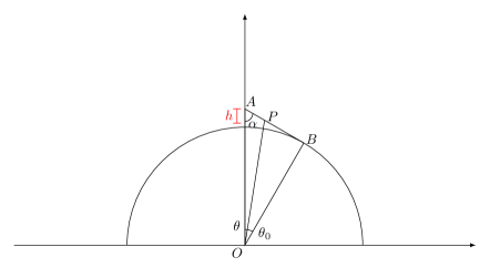
Figure 1. External tangent case

We have that

$$h+1=\dfrac{1}{\cos(\theta_{0})}.$$ (3.9)

Let $\theta\in(0,\theta_{0})$. Having $u(\theta)=1/r(\theta)$, using the sine theorem to the triangle $OAP$, we obtain

$$u(\theta)=\cos(\theta_{0}-\theta).$$ (3.10)

and, consequently,

$$u^{\prime}(\theta)=-\sin(\theta_{0}-\theta).$$ (3.11)

Using (3.11) and Taylor expanding up to the first order with respect to $\theta_{0}$, we have that

$$\int_{0}^{\theta_{0}}\left(u^{\prime}(\theta)\right)^{2}d\theta=\int_{0}^{\theta_{0}}\sin^{2}(\theta_{0}-\theta)\>d\theta=\left[\frac{\theta_{0}}{2}-\dfrac{\sin(2\theta_{0})}{4}\right]\approx\,\frac{2\theta_{0}^{3}}{3}$$ (3.12)

and

$$\displaystyle\int_{0}^{\theta_{0}}|1-u(\theta)|\;d\theta=\displaystyle\int_{0}^{\theta_{0}}\left(1-u(\theta)\right)d\theta=\displaystyle\int_{0}^{\theta_{0}}\left(1-\cos(\theta_{0}-\theta)\right)d\theta=$$ (3.13)

$$=\left(\theta_{0}-\sin(\theta_{0})\right)\approx\dfrac{\theta_{0}^{3}}{6}.$$ (3.14)

So, there exists a non negative constant $C$ such that

$$\int_{0}^{\theta_{0}}|1-u(\theta)|\;d\theta\geq C\int_{0}^{\theta_{0}}\left(u^{\prime}(\theta)\right)^{2}d\theta.$$

Case 2: External Secant. We are now considering the case when $\alpha+\theta_{0}<\pi/2$, the segment $\overline{OB}$ has length $1$ and the side of the polygon $\overline{AB}$ is external to the unitary ball and touches it in the point $B$.

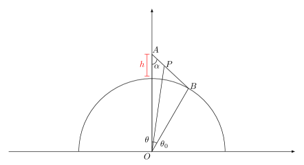
Figure 2. External Secant Case

We set $z=\pi/2-\alpha$ and in this case we have that

$$h+1=\dfrac{\sin(\alpha+\theta_{0})}{\sin(\alpha)}$$ (3.15)

and, using the sine theorem to the triangle $OAP$,

$$u(\theta)=\dfrac{\sin(\alpha+\theta)}{\sin(\alpha)(h+1)}$$ (3.16)

and so

$$u^{\prime}(\theta)=\dfrac{\cos(\alpha+\theta)}{\sin(\alpha)(h+1)}.$$ (3.17)

Denoting by $I=1/\left(\sin(\alpha)(h+1)\right)$ and Taylor expanding up to the first order with respect to $\theta_{0}$ and to $z$, we have that

$$\int_{0}^{\theta_{0}}\left(u^{\prime}(\theta)\right)^{2}d\theta=I^{2}\left(\frac{\theta_{0}}{2}+\dfrac{\sin(2z-2\theta_{0})}{4}-\dfrac{\sin(2z)}{4}\right)\simeq\frac{I^{2}}{3}\left[3z^{2}\theta_{0}-3z\theta_{0}^{2}+\theta_{0}^{3}\right].$$ (3.18)

and, using (3.15),

$$\displaystyle\int_{0}^{\theta_{0}}|1-u(\theta)|\;d\theta=\displaystyle\int_{0}^{\theta_{0}}\left(1-u(\theta)\right)d\theta=I\displaystyle\int_{0}^{\theta_{0}}\left(1-\dfrac{\cos(\theta_{0}-\theta)}{(h+1)\sin(\alpha)}\right)d\theta=$$

$$= I\left[\sin(\alpha)(h+1)\theta_{0}+\cos(\alpha+\theta_{0})-\cos(\alpha)\right]=$$

$$=I\left[\theta_{0}\cos(\theta_{0}-z)+\sin(z)\left(\cos(\theta_{0})-1\right)-\cos(z)\sin(\theta_{0})\right]\simeq\dfrac{3I}{2}\left[3z\theta_{0}^{2}-2\theta_{0}^{3}\right].$$

Since we can choose $\theta_{0}$ such that $z>(2/3)\theta_{0}$, from the last two relations, we can conclude that there exists a non negative constant $C$ such that

$$\int_{0}^{\theta_{0}}|1-u(\theta)|\;d\theta\geq C\int_{0}^{\theta_{0}}\left(u^{\prime}(\theta)\right)^{2}d\theta.$$

Case 3: External not Intersecting. We are considering the case when $\alpha+\theta_{0}\leq\pi/2$, the segment $\overline{OB}$ has length strictly greater than $1$ and the side of the polygon $\overline{AB}$ is external to the unitary ball.

Figure 3. External not intersecting case

We set $z=\pi/2-\alpha$ and we consider the line $\mathit{r}$ intersecting the segment $\overline{OA}$, that is parallel to the line passing through the points $A$ and $B$ and that touches the ball. We call $h$ the length of the segment $\overline{AQ}$, where $Q$ is the point of intersection between the segment $\overline{AO}$ and the line $\mathit{r}$ and we call $h^{\prime}$ the length of the segment $\overline{QQ^{\prime}}$, where $Q^{\prime}$ is the the point of intersection between the segment $\overline{AO}$ and the ball. Let us first assume that $\alpha+\theta_{0}=\pi/2$. We have that

$$u(\theta)=\dfrac{\cos(\theta_{0}-\theta)}{\sin(\alpha)(h+h^{\prime}+1)}.$$ (3.19)

So, setting $I=1/\left(\sin(\alpha)(h+h^{\prime}+1)\right)$, we obtain that

$$\int_{0}^{\theta_{0}}\left(u^{\prime}(\theta)\right)^{2}d\theta=I^{2}\int_{0}^{\theta_{0}}\sin^{2}(\theta-\theta_{0})\>d\theta=I^{2}\left(\dfrac{\theta_{0}}{2}-\dfrac{\sin(2\theta_{0})}{4}\right)\approx I^{2}\frac{4}{3}\theta_{0}^{3}.$$ (3.20)

Let us denote by $A_{T}$ the area of the trapeze $ABTQ$ and let us compute $A_{T}$:

$$A_{T}=\dfrac{\sin(\theta_{0})(1+2h+h^{\prime})}{2}h^{\prime}\cos(\theta_{0})\approx\frac{h^{\prime}}{2}\sin(2\theta_{0})\approx\frac{h^{\prime}}{2}(2\theta_{0}-\frac{4\theta^{3}_{0}}{3}).$$ (3.21)

So, since

$$\int_{0}^{\theta_{0}}(1-u(\theta))\;d\theta\geq A_{T},$$

we can conclude that there exists a costant $C>0$ such that

$$\int_{0}^{\theta_{0}}|1-u(\theta)|\;d\theta\geq C\int_{0}^{\theta_{0}}\left(u^{\prime}(\theta)\right)^{2}d\theta.$$

Now let us assume that $\alpha+\theta_{0}>\pi/2$ and let us set $z=\pi/2-\alpha$. We have that

$$u(\theta)=\dfrac{\sin(\theta+\alpha)}{\sin(\alpha)(h+h^{\prime}+1)}$$ (3.22)

and that

$$\dfrac{1}{I^{2}}\int_{0}^{\theta_{0}}\left(u^{\prime}(\theta)\right)^{2}d\theta=\int_{0}^{\theta_{0}}\sin^{2}(\theta+\alpha)\>d\theta=\dfrac{\theta_{0}}{2}-\dfrac{\sin(2\theta_{0}+2\alpha)}{4}+\dfrac{\sin(2\alpha)}{4}$$

$$=\dfrac{\theta_{0}}{2}+\dfrac{\sin(2z)}{4}\left(1-\cos(2\theta_{0})\right)+\dfrac{cos(2z)\sin(2\theta_{0})}{4}\approx\theta_{0}+\theta_{0}^{2}z-z^{2}\theta_{0}-\frac{2}{3}\theta_{0}^{3}.$$

If we compute $A_{T}$:

$$A_{T}=\frac{\sin(\theta_{0})}{2}[\sin^{2}(\alpha)\sin^{2}(\beta)+\sin^{3}(\alpha)\sin(\beta)(1+h+h^{\prime})]$$

and we can conclude.

Case $3$: Internal not Touching. Let us assume that the segments $\overline{OA}$ and $\overline{OB}$ are both less than $1$ and we call $h:=1-|\overline{OA}|$ and $\beta$ the angle $O\hat{B}A$

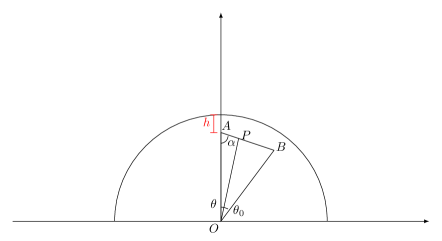
Figure 4. Internal not intersecting case

In this case we have that

$$u(\theta)=\dfrac{\sin(\alpha+\theta)}{(1-h)\sin(\alpha)}.$$

Setting $I=1/(1-h)\sin(\alpha)$ and $z=\pi/2-\alpha$,

$$\dfrac{1}{I^{2}}\int_{0}^{\theta_{0}}\left(u^{\prime}(\theta)\right)^{2}d\theta=\dfrac{\theta_{0}^{2}}{2}+\dfrac{\sin(2z-2\theta_{0})}{4}-\dfrac{\sin(2z)}{4}\approx\dfrac{\theta^{3}_{0}}{3}-z\theta_{0}^{2}+z^{2}\theta_{0}.$$

Let $Q$ be the point that lays in the circumference and in the semi-line that contains the segment $\overline{OA}$ and $Q^{\prime}$ a point that lays in the semi-line containing $\overline{OB}$, such that the segment $\overline{QQ^{\prime}}$ is parallel to $\overline{AB}$. Calling $A_{T}$ the area of the trapeze $ABQQ^{\prime}$, we have

$$A_{T}=\dfrac{h(2-h)\sin(\alpha)}{2\sin(\beta)}\sin(\theta_{0}).$$

We can conclude, since

$$\int_{0}^{\theta_{0}}|1-u(\theta)|\;d\theta\geq A_{T}.$$

Case $4$: Internal Touching. Let us assume that the side $\overline{AB}$ is now contained in the ball and that the segment $\overline{OB}$ has length less than $1$.

Figure 5. Internal secant case

In this case, setting $I=1/\sin(\alpha)$ and $z=\pi/2-\alpha$, we have, when $z\to 0$ that

$$\dfrac{1}{I^{2}}\int_{0}^{\theta_{0}}\left(u^{\prime}(\theta)\right)^{2}d\theta=\int_{0}^{\theta_{0}}\cos^{2}(\theta+\alpha)\>d\theta=\frac{\theta_{0}}{2}+\dfrac{\sin(2z-2\theta_{0})}{4}-\dfrac{\sin(2z)}{4}$$

$$\approx\frac{\theta_{0}^{3}}{3}+z^{2}\theta_{0}-z\theta_{0}^{2}$$

and

$$\dfrac{1}{I}\displaystyle\int_{0}^{\theta_{0}}(u(\theta)-1)\;d\theta=-\sin(z-\theta_{0})+\sin(z)-\theta_{0}\cos(z)\approx\dfrac{z\theta_{0}^{2}}{2}-\dfrac{\theta_{0}^{3}}{6},$$

and we can conclude, since we can show after some computations of Euclidean geometry that $z$ goes to $0$ with the same speed as $\theta_{0}$. If we are in the case that $z$ does not tend to $0$, as $\theta_{0}\to 0$, we Taylor expand in $\theta_{0}$ and we easily obtain the desired result. ∎

3.2. Proof of Proposition 3.1 in the higher dimensional case

We can assume that the boundary of $\Omega\in\mathcal{C}_{n}$ can be parametrized as in (2.4) and we can argue as in Section 3.1 (using the results contained in [13]): for every $\varepsilon>0$, there exists a positive constant $\delta$, depending only on the dimension $n$ such that, if $\Delta P(\Omega)\leq\delta$ , then $||1-r||_{L^{\infty}(\mathbb{S}^{n-1})}\leq\varepsilon$. Now, from (2.5), we have that

$$\mathcal{A}_{F}(\Omega)\leq\frac{n+1}{n}\int_{\mathbb{S}^{n-1}}|r(x)-1|\;d\mathcal{H}^{n-1}.$$ (3.23)

So, by (3.23) and (2.6), proving Proposition 3.1, is equivalent to prove that there exists $C>0$ such that

$$\int_{\mathbb{S}^{n-1}}|r(x)-1|\;d\mathcal{H}^{n-1}\geq C\int_{\mathbb{S}^{n-1}}\left[|\nabla_{\tau}r|^{2}+r^{2}-\dfrac{1}{r^{2(n-2)}}\right]\;d\mathcal{H}^{n-1}.$$ (3.24)

We note now that

$$r^{2}-\dfrac{1}{r^{2(n-2)}}=\dfrac{\left(r-1\right)}{r^{2(n-2)}}\left(1+r+\cdots r^{2n-3}\right).$$

and the term

$$\dfrac{1}{r^{2(n-2)}}\left(1+r+\cdots r^{2n-3}\right)$$

is bounded if $||1-r||_{L^{\infty}(\mathbb{S}^{n-1})}\leq\varepsilon$, so that it can absorbed by the constant $C$. For this reason, it remains to prove

$$\int_{\mathbb{S}^{n-1}}|r(x)-1|\;d\mathcal{H}^{n-1}\geq C\int_{\mathbb{S}^{n-1}}|\nabla_{\tau}r|^{2}\;d\mathcal{H}^{n-1},$$

that is the claim of the following proposition.

Lemma 3.4.

Let $n>2$. There exist $C>0$, depending only on $n$, such that, for every $\Omega\in\mathcal{C}_{n}$ with $\Delta P(\Omega)<\delta$, then, if $r$ is the function that describes the boundary of $\Omega$ as defined in (2.4), it holds

$$\int_{\mathbb{S}^{n-1}}|r(x)-1|\;d\mathcal{H}^{n-1}(x)\geq C\int_{\mathbb{S}^{n-1}}|\nabla_{\tau}r(x)|^{2}\;d\mathcal{H}^{n-1}(x).$$ (3.25)

Proof.

We fix a system of coordinates $\left(O,e_{1},\cdots,e_{n}\right)$ and we prove the desired inequality in a neighbourhood $\omega$ of the point $x_{0}:=(0,\cdots,0,1)$.
Let $x\in\omega$, there exists $c>0$ such that

$$|\nabla_{\tau}r(x)|^{2}\leq c\sum_{i=1}^{n-1}|\nabla_{i}r(x)|^{2},$$ (3.26)

where $\nabla_{i}u(x)$ is the tangential gradient of $u$ in the circle $C_{i}$, that is the circle given by the intersection of $\mathbb{S}^{n-1}$ and the plane that contains the origin $O$ and the vectors $x$ and $e_{i}$, for every $i=1,\dots,n-1$. Inequality (3.26) is an easy consequence of the fact that the tangent $\tau_{i}$ at $C_{i}$ in $x$ are almost orthogonal. We prove now the following inequality: there exists a constant $C>0$ such that

$$\int_{\omega}|r(x)-1|\;d\mathcal{H}^{n-1}(x)\geq C\int_{\omega}|\nabla_{n-1}r|^{2}\;d\mathcal{H}^{n-1}(x).$$ (3.27)

In order to do that, we consider the spherical coordinates of $\mathbb{S}^{n-1}$:

$$\begin{cases}x_{1}=\cos(\theta_{1})\\ x_{2}=sin(\theta_{1})\cos(\theta_{2})\\ \vdots\\ x_{n-1}=\sin(\theta_{1})\dots\sin(\theta_{n-2})\cos(\theta_{n-1})\\ x_{n}=\sin(\theta_{1})\dots\sin(\theta_{n-2})\sin(\theta_{n-1})\end{cases}$$

with $\theta_{1}\dots,\theta_{n-2}\in[0,\pi]$ and $\theta_{n-1}\in[0,2\pi)$. In this coordinate system the point $x_{0}=(0,\cdots,0,1)$ corresponds to

$$\theta_{1}=\pi/2,$$

$$\theta_{2}=\pi/2,$$

$$\vdots$$

$$\theta_{n-1}=\pi/2.$$

We fix now $\theta_{1},\dots,\theta_{n-2}$ and we let $\theta_{n-1}$ vary in a small interval $[\pi/2-\delta_{1},\pi/2+\delta_{1}]$. We write on the the piece of circle $\omega^{\prime}$ described by this parametrization the bidimensional inequality that we have proved in the previous Section 3.1

$$\int_{\omega^{\prime}}|r(x)-1|\;d\mathcal{H}^{1}\geq C\int_{\omega^{\prime}}|\nabla_{n-1}r|^{2}\;d\mathcal{H}^{1}.$$ (3.28)

Now we multiply both sides of (3.28) by the corresponding Jacobian

$$\left(\sin^{n-2}(\theta_{1})\sin^{n-3}(\theta_{2})\dots\sin(\theta_{n-2})\right)$$

and we integrate in $\theta_{1},\theta_{2},\dots,\theta_{n-2}$ in a small neighbourhood, proving in this way inequality (3.27). In a similar way, with a suitable choice of spherical coordinates, we prove that for $i=1,\dots,n-2$, also holds

$$\int_{\omega}|r(x)-1|\;d\mathcal{H}^{n-1}(x)\geq C\int_{\omega}|\nabla_{i}r|^{2}\;d\mathcal{H}^{n-1}(x).$$ (3.29)

Summing and using (3.26), we can conclude that

$$\int_{\omega}|r(x)-1|\;d\mathcal{H}^{n-1}(x)\geq C\int_{\omega}|\nabla_{\tau}r|^{2}\;d\mathcal{H}^{n-1}(x).$$ (3.30)

∎

4. Proof of the Theorem 1.3

Proof.

From (2.28), it follows that there exists a constant $K_{n}>0$ such that

$$\Delta\lambda_{1}(\Omega)\geq K\left(P(\Omega)\right)^{2}-\lambda_{1}(B).$$

Let us define the function $f_{1}:\mathbb{R}\to\mathbb{R}$ as

$$f_{1}(x)=\dfrac{Kx^{2}-\lambda_{1}(B)}{Kx^{2}}.$$

Since

$$\lim_{x\to+\infty}f_{1}(x)=1,$$

we have that there exists $M_{1}>0$ such that, if $x>M_{1}+P(B)$, then $f_{1}(x)\geq 1/2$. This is equivalent to say that, if $\Delta P(\Omega)>M_{1}$, then

$$\Delta\lambda_{1}(\Omega)\geq\dfrac{K}{2}P(\Omega)^{2}=\dfrac{K}{2}\left(\dfrac{\Delta P(\Omega)+P(B)}{\Delta P(\Omega)}\right)^{2}\Delta P(\Omega)^{2}.$$

If we define now

$$f_{2}(x)=\dfrac{x+P(B)}{x},$$

being $\lim_{x\to+\infty}f_{2}(x)=1$, we have that there exists $M_{2}>M_{1}$ such that, if $x>M_{2}$ then $f_{2}(x)\geq 1/2$. This means that, if $\Delta P(\Omega)>M_{2}$ then

$$\Delta\lambda_{1}(\Omega)\geq\dfrac{K}{8}\Delta P(\Omega)^{2}.$$ (4.1)

Let us assume now that we are in the case $\Delta P(\Omega)<\delta$. We can combine the sharp quantitative Faber-Krahn inequality (2.26) with Proposition 3.1 and we obtain

$$\Delta\lambda_{1}(\Omega)\geq\bar{C}\mathcal{A}^{2}_{F}(\Omega)\geq C^{2}\;\bar{C}\Delta P(\Omega)^{2}.$$ (4.2)

It remains to study the intermediate case $\delta<\Delta P(\Omega)\leq M_{2}$. Combining (2.27) and (2.5), we obtain

$$\dfrac{\Delta\lambda_{1}(\Omega)}{\left(\Delta P(\Omega)\right)^{2}}\geq\dfrac{M\mathcal{A}_{H}(\Omega)^{2n^{2}}}{M^{2}_{2}}\geq\dfrac{MK\left(\Delta P(\Omega)P(\Omega)^{(2-n)/(n-1)}\right)^{2n^{2}}}{M_{2}^{2}}\geq\dfrac{\alpha}{M_{2}^{2}},$$ (4.3)

where we have assumed, without loss of generality, that the ball centered at the origin is the one that achieves the minimum in (2.3) and

$$\alpha:=MK\left(\left(M_{2}+P(B)\right)^{(2-n)/(n-1)}\delta\right)^{2n^{2}}.$$

We conclude the proof of Theorem 1.3, choosing the constant $c=c(n)>0$ by taking the minimum between the constant in (4.1), (4.2) and (4.3):

$$c_{n}=\min\left\{\dfrac{K}{8},\;C^{2}\bar{C},\;\dfrac{\alpha}{M_{2}^{2}}\right\}.$$ (4.4)

∎

We conclude with the following Remark.

Remark 4.1.

Proceeding in this way, by using the sharp inequality proved in [6], we are not able to prove the conjectured inequality (1.2): our leading idea is indeed to combine th quantitative Faber-Krahn inequality (2.26) with an inequality of the form

$$\mathcal{A}_{\mathcal{F}}(\Omega)\geq C\left(P(\Omega)-P(B)\right)^{\delta},$$ (4.5)

$\delta>0.$ In this case, the target power in (4.5) to prove (1.2) would be $3/4$, but, unfortunately, the best power is $\delta=1$ and the ”bad” sets are in this case the polygons, as pointed out in Remark 3.2.

References

- [1] P. Antunes, P. Freitas, New bounds for the principal Dirichlet eigenvalue of planar regions, Experimental Mathematics, 15 (3), 333-342 (2006).
- [2] G. Bellettini, Lecture Notes on Mean Curvature Flow: Barriers and Singular Perturbations. Lecture Notes Scuola Normale Superiore (2013).
- [3] L. Brasco, On principal frequencies and inradius in convex sets, Bruno Pini Math. Anal. Semin., 9, 78-101 (2018).
- [4] L. Brasco, G. De Philippis, Spectral inequalities in quantitative formShape optimization and spectral theory, 201?281, De Gruyter Open, Warsaw, (2017).
- [5] L. Brasco, G. De Philippis, B. Rufini, Spectral optimization for the Stekloff–Laplacian: the stability issue, Journal of Functional Analysis, 262, 4675-4710 (2012).
- [6] L. Brasco, G. De Philippis, B. Velichkov, Faber-Krahn inequalities in sharp quantitative form, Duke Math. J., Volume 164, Number 9, 1777-1831(2015).
- [7] Z. Chen, Z. Chen, The Lp Minkowski problem for q-capacity Proceedings of the Royal Society of Edinburgh Section A: Mathematics (to appear): 1-31.
- [8] L. Esposito, N. Fusco, C. Trombetti, A quantitative version of the isoperimetric inequality: the anisotropic case, Ann. Sc. Norm. Super. Pisa Cl. Sci. 4, 619-651 (2005).
- [9] L.C. Evans, R.F. Gariepy, Measure theory and fine properties of functions, CRC Press, Inc., Boca Raton, Florida, (1992).
- [10] G. Faber, Beweis, dass unter allen homogenen Membranen von gleicher Fläche und gleicherSpannung die kreisförmige den tiefsten Grundton gibt.Verlagd, Verlagd. Bayer. Akad. d. Wiss., 8,(1923).
- [11] I. Ftouhi, J. Lamboley, Blaschke-Santaló diagram for volume, perimeter and first Dirichlet eigenvalue, SIAM Journal on Mathematical Analysis, Society for Industrial and Applied Mathematics, (2020).
- [12] N. Fusco, The stability of the isoperimetric inequality for convex or nearly spherical domains in . Lecture Notes in Math., Springer, 2179, 73-123 (2017).
- [13] N. Fusco, M. S. Gelli, G. Pisante, On a Bonnesen type inequality involving the spherical deviation, J. Math. Pures Appl. (9) 98, no. 6, 616-632 (2012).
- [14] N. Fusco, F. Maggi, A. Pratelli, The sharp quantitative isoperimetric inequality, Annals of Mathematics, 168, 941-980 (2008).
- [15] N. Fusco, F. Maggi, A. Pratelli, Stability estimates for certain Faber-Krahn, Isocapacitary and Cheeger inequalities, Ann. Sc. Norm. Super. Pisa Cl. Sci., 8, 51-71 (2009).
- [16] P. Grinfeld, G. Strang, The Laplace eigenvalue of a polygon, Computers & Mathematics with Applications, Elsevier, 48, 1121-1133, (2004).
- [17] P. Grinfeld, G. Strang, Laplace eigenvalues on regular polygons: a series in , Journal of Mathematical Analysis and Applications 385(1):135-149, (2012).
- [18] J. Lamboley, A. Novrouzi, M. Pierre, Regularity and Singularities of Optimal Convex Shape in the Plane, Arch. Ration. Mech. Anal. 205, no. 1, 311-343 (2012).
- [19] S. Kesevan, Symmetrization and applications, Series in Analysis, 3. Word Scientific Pubblishing Co. Pte. Ltd., Hackensack, NJ, (2006).
- [20] E. Krahn., Über eine von Rayleigh formulierte Minimaleigenschaft des Kreises, Math. Ann.,94(1):97?100, (1925).
- [21] A. Henrot, Extremum problems for eigenvalues of elliptic operators, Frontiers in mathematics. Birkhauser Verlag, Basel, (2006).
- [22] F. Maggi, Sets of Finite Perimeter and Geometric Variational Problems: An Introduction to Geometric Measure Theory, Cambridge Studies in Advanced Mathematics (2012).
- [23] A. Melas, The stability of some eigenvalue estimates, J. Differential Geom. 36, no. 1, 19?33 (1992).
- [24] L. Molinari, On the ground state of regular polygonal billiards, Journal of Physics A: Mathematical and General, 30(18):6517, (1997).
- [25] C. Nitsch, An isoperimetric result for the fundamental frequency via domain derivative, Calc. Var. Partial Differential Equations 49, no. 1-2, 323-335(2014).
- [26] G. Pólya, G. Szegö, Isoperimetric Inequalities in Mathematical Physics. Annals of Mathematics Studies, no. 27, Princeton University Press, Princeton, N. J. (1951).
- [27] R. Schneider, Convex bodies: the Brunn-Minkowski theory. Second expanded edition, Encyclopedia of Mathematics and its Applications, 151.Cambridge University Press, Cambridge (2014).