Odd Microswimmer

Abstract

We propose a model for a thermally driven microswimmer in which three spheres are connected by two springs with odd elasticity. We demonstrate that the presence of odd elasticity leads to the directional locomotion of the stochastic microswimmer.

Although micromachines such as proteins and enzymes experience the influence of strong thermal fluctuations, they often exhibit directional locomotion under nonequilibrium conditions Yuan21 . To elucidate this type of phenomena, we previously proposed a thermally driven elastic microswimmer consisting of three spheres Hosaka17 . In this model, the three spheres were assumed to be in equilibrium with independent heat baths characterized by different temperatures.

Recently, Scheibner et al. introduced the concept of “odd elasticity,” which can arise from active and nonreciprocal interactions Scheibner20 . Importantly, the odd part of the elastic constant tensor quantifies the amount of work extracted along quasistatic deformation cycles. In this paper, we propose a novel type of thermally driven microswimmer in which the three spheres are connected with springs having not only even elasticity Yasuda17 , but also odd elasticity Scheibner20 . We explicitly demonstrate that the proposed stochastic “odd microswimmer” can exhibit a directional locomotion as a result of odd elasticity. Additionally, we provide a simple physical interpretation of the average velocity within the nonequilibrium statistical physics.

Consider a three-sphere microswimmer in which the positions of the three spheres of radius $a$ are given by $x_{i}$ ($i=1,2,3$) in a one-dimensional coordinate system (see Fig. 1) Golestanian08 . These three spheres are connected by two springs that exhibit both even and odd elasticity. We denote the two spring extensions as $u_{\mathrm{A}}=x_{2}-x_{1}-\ell$ and $u_{\mathrm{B}}=x_{3}-x_{2}-\ell$, where $\ell$ is the natural length. Then, the forces $F_{\mathrm{A}}$ and $F_{\mathrm{B}}$ conjugate to $u_{\mathrm{A}}$ and $u_{\mathrm{B}}$, respectively, are given by $F_{\alpha}=-K_{\alpha\beta}u_{\beta}$ ($\alpha,\beta=\mathrm{A},\mathrm{B}$). For an odd spring, the elastic constant $K_{\alpha\beta}$ is given by Scheibner20

$$K_{\alpha\beta}=K^{\mathrm{e}}\delta_{\alpha\beta}+K^{\mathrm{o}}\epsilon_{\alpha\beta},$$ (1)

where $K^{\mathrm{e}}$ and $K^{\mathrm{o}}$ are the even and odd elastic constants, respectiverly, in the 2D configuration space spanned by $u_{\mathrm{A}}$ and $u_{\mathrm{B}}$ (unlike the real 2D space in Ref. Scheibner20 , $\delta_{\alpha\beta}$ is the Kronecker delta, and $\epsilon_{\alpha\beta}$ is the 2D Levi-Civita tensor with $\epsilon_{\mathrm{AA}}=\epsilon_{\mathrm{BB}}=0$ and $\epsilon_{\mathrm{AB}}=-\epsilon_{\mathrm{BA}}=1$. The presence of odd elasticity $K^{\mathrm{o}}$ in Eq. (1) reflects the nonreciprocal interaction between the two springs such that $u_{\mathrm{A}}$ and $u_{\mathrm{B}}$ influence each other in a different manner Era21 . The forces $f_{i}$ acting on each sphere are given by $f_{1}=-F_{\mathrm{A}}$, $f_{2}=F_{\mathrm{A}}-F_{\mathrm{B}}$, and $f_{3}=F_{\mathrm{B}}$. These forces satisfy the force-free condition, i.e., $f_{1}+f_{2}+f_{3}=0$.

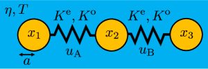
Figure 1: (Color online) Odd microswimmer in a fluid with a viscosity $\eta$ and temperature $T$. Three spheres of radius $a$ are connected by two springs with a natural length $\ell$. Each spring has both even elastic constant $K^{\mathrm{e}}$ and odd elastic constant $K^{\mathrm{o}}$. The positions of the spheres are denoted as $x_{i}$ ($i=1,2,3$), and the spring extensions with respect to $\ell$ are denoted as $u_{\mathrm{A}}$ and $u_{\mathrm{B}}$.

The odd microswimmer described above is immersed in a fluid with a shear viscosity of $\eta$ and temperature $T$. Then the equations of motion for each sphere are given by Hosaka17 ; Yasuda17 ; Golestanian08

$$\dot{x}_{i}=M_{ij}f_{j}+\xi_{i},$$ (2)

where $\dot{x}_{i}=dx_{i}/dt$ and $M_{ij}$ are the hydrodynamic mobility coefficients Golestanian08

$$M_{ij}=\begin{cases}1/(6\pi\eta a)&(i=j)\\ 1/(4\pi\eta\,|x_{i}-x_{j}|)&(i\neq j)\end{cases}.$$ (3)

In Eq. (2), the Gaussian white-noise sources $\xi_{i}$ have zero mean $\langle\xi_{i}(t)\rangle=0$, and their correlations satisfy the following fluctuation-dissipation theorem:

$$\langle\xi_{i}(t)\xi_{j}(t^{\prime})\rangle=2k_{\mathrm{B}}TM_{ij}\delta(t-t^{\prime}),$$ (4)

where $k_{\mathrm{B}}$ is the Boltzmann constant.

It is convenient to introduce a characteristic time scale $\tau=6\pi\eta a/K^{\mathrm{e}}$ and the ratio between the two spring constants $\lambda=K^{\mathrm{o}}/K^{\mathrm{e}}$. In the following analysis, we assume $u_{\mathrm{A}},u_{\mathrm{B}}\ll\ell$ and $a\ll\ell$, and focus solely on the leading-order contribution. The total velocity of the microswimmer is given by $V=(\dot{x}_{1}+\dot{x}_{2}+\dot{x}_{3})/3$. After taking the statistical average and using Eqs. (1)-(3), we obtain Hosaka17

$$\langle V\rangle =\frac{a}{8\ell^{2}\tau}\left[\langle u_{\mathrm{B}}^{2}\rangle-\langle u_{\mathrm{A}}^{2}\rangle+\lambda\left(3\langle u_{\mathrm{B}}^{2}\rangle+3\langle u_{\mathrm{A}}^{2}\rangle-2\langle u_{\mathrm{A}}u_{\mathrm{B}}\rangle\right)\right]$$

$$+\mathcal{O}[(a/\ell)^{2},(u/\ell)^{3}],$$ (5)

where we use $\langle u_{\mathrm{A}}\rangle=\langle u_{\mathrm{B}}\rangle=0$.

The equal-time correlation functions appearing in Eq. (5) can be obtained from the reduced Langevin equations for $\dot{u}_{\mathrm{A}}=\dot{x}_{2}-\dot{x}_{1}$ and $\dot{u}_{\mathrm{B}}=\dot{x}_{3}-\dot{x}_{2}$ as

$$\dot{u}_{\alpha}=\Gamma_{\alpha\beta}u_{\beta}+\Xi_{\alpha}+\mathcal{O}[a/\ell],$$ (6)

where $\Gamma_{\alpha\beta}$ and $\Xi_{\alpha}$ are

$$\mathbf{\Gamma}=-\frac{1}{\tau}\left(\begin{array}[]{ccc}2+\lambda&-1+2\lambda\\ -1-2\lambda&2-\lambda\end{array}\right),~{}~{}~{}\mathbf{\Xi}=\left(\begin{array}[]{cc}\xi_{2}-\xi_{1}\\ \xi_{3}-\xi_{2}\end{array}\right).$$ (11)

Notice that $\Gamma_{\alpha\beta}$ is nonreciprocal, i.e., $\Gamma_{\mathrm{AB}}\neq\Gamma_{\mathrm{BA}}$ when $\lambda\neq 0$. By solving Eq. (6) in the Fourier domain and using Eq. (4), we obtain the following equal-time correlation functions Hosaka17 :

$$\langle u_{\mathrm{A}}^{2}\rangle=\frac{k_{\mathrm{B}}T}{K^{\mathrm{e}}}\left[1-\frac{\lambda}{2(1+\lambda^{2})}\right]+\mathcal{O}[a/\ell],$$ (12)

$$\langle u_{\mathrm{B}}^{2}\rangle=\frac{k_{\mathrm{B}}T}{K^{\mathrm{e}}}\left[1+\frac{\lambda}{2(1+\lambda^{2})}\right]+\mathcal{O}[a/\ell],$$ (13)

$$\langle u_{\mathrm{A}}u_{\mathrm{B}}\rangle=-\frac{k_{\mathrm{B}}T}{K^{\mathrm{e}}}\frac{\lambda^{2}}{2(1+\lambda^{2})}+\mathcal{O}[a/\ell].$$ (14)

Here, we neglect the cross-correlations $\langle\xi_{i}\xi_{j}\rangle$ with $i\neq j$ because they only contribute to higher orders in $a/\ell$. When $\lambda=0$, the above expressions reduce to $\langle u_{\mathrm{A}}^{2}\rangle=\langle u_{\mathrm{B}}^{2}\rangle=k_{\mathrm{B}}T/K^{\mathrm{e}}$ and $\langle u_{\mathrm{A}}u_{\mathrm{B}}\rangle=0$, reproducing the thermal equilibrium situation. We have $\langle u_{\mathrm{A}}^{2}\rangle<\langle u_{\mathrm{B}}^{2}\rangle$ when $\lambda>0$, because the effective elastic constant of spring A is greater than that of spring B.

By substituting Eqs. (12)-(14) into Eq. (5), we obtain the average velocity as

$$\langle V\rangle=\frac{7ak_{\mathrm{B}}T\lambda}{8\ell^{2}K^{\mathrm{e}}\tau}+\mathcal{O}[(a/\ell)^{2},(u/\ell)^{3}].$$ (15)

Here, $\langle V\rangle$ is proportional to the odd elastic constant $K^{\mathrm{o}}$ that can take either positive or negative value. Because $\langle V\rangle$ is also proportional to $k_{\mathrm{B}}T$, thermal fluctuations are responsible for the locomotion of the odd microswimmer. Therefore, our model provides a novel type of Brownian ratchet.

Next, we discuss the nonequilibrium statistical properties of the odd microswimmer Sou19 ; Sou21 . For the time-dependent probability distribution function $p(u_{\mathrm{A}},u_{\mathrm{B}},t)$, the Fokker-Planck equation corresponding to Eq. (6) can be written as $\dot{p}=-\partial_{\alpha}j_{\alpha}$, where $\partial_{\alpha}=\partial/(\partial u_{\alpha})$ and $j_{\alpha}$ is the probability flux given by Sou19

$$j_{\alpha}=\Gamma_{\alpha\beta}u_{\beta}p-D_{\alpha\beta}\partial_{\beta}p.$$ (16)

Here, $D_{\alpha\beta}$ is the diffusion matrix

$$\mathbf{D}=\frac{k_{\mathrm{B}}T}{6\pi\eta a}\left(\begin{array}[]{cc}2&-1\\ -1&2\end{array}\right),$$ (19)

which satisfies the relationship $\langle\Xi_{\alpha}(t)\Xi_{\beta}(t^{\prime})\rangle=2D_{\alpha\beta}\delta(t-t^{\prime})$ according to Eq. (4).

Owing to the reproductive property of Gaussian distributions, the steady-state probability distribution function that satisfies $\dot{p}=0$ is given by a Gaussian function Sou19

$$p(u_{\mathrm{A}},u_{\mathrm{B}})=\frac{1}{2\pi\sqrt{\det\mathbf{C}}}\exp\left[-\frac{1}{2}(C^{-1})_{\alpha\beta}u_{\alpha}u_{\beta}\right].$$ (20)

Here, $C_{\alpha\beta}=\langle u_{\alpha}u_{\beta}\rangle$ is the covariance matrix obtained from Eqs. (12)-(14) as

$$\mathbf{C}=\frac{k_{\mathrm{B}}T}{K^{\mathrm{e}}}\frac{1}{1+\lambda^{2}}\left(\begin{array}[]{cc}1-\lambda/2+\lambda^{2}&-\lambda^{2}/2\\ -\lambda^{2}/2&1+\lambda/2+\lambda^{2}\end{array}\right),$$ (23)

and $(C^{-1})_{\alpha\beta}$ is the inverse matrix of $C_{\alpha\beta}$. For our purposes, we explicitly show that

$$\det\mathbf{C}=\left(\frac{k_{\mathrm{B}}T}{K^{\mathrm{e}}}\right)^{2}\frac{4+7\lambda^{2}+3\lambda^{4}}{4(1+\lambda^{2})^{2}}.$$ (24)

In Fig. 2, we plot the steady-state probability distribution function in Eq. (20) and corresponding probability flux in Eq. (16) when $\lambda=1$. The probability distribution function is distorted by the negative correlation ($C_{\mathrm{AB}}=C_{\mathrm{BA}}\sim-\lambda^{2}/2$) between $u_{\mathrm{A}}$ and $u_{\mathrm{B}}$. One can see a counter-clockwise loop of the probability flux. Such a probability flux becomes clockwise for $\lambda<0$ and vanishes when $\lambda=0$. The existence of a probability flux loop indicates that the detailed balance is broken in the nonequilibrium steady state.

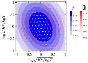
Figure 2: (Color online) Steady-state scaled probability distribution function $\tilde{p}=pk_{\mathrm{B}}T/K^{\mathrm{e}}$ and steady-state scaled probability flux $\tilde{\mathbf{j}}=\mathbf{j}\tau\sqrt{k_{\mathrm{B}}T/K^{\mathrm{e}}}$ (arrows) in the configuration space spanned by $u_{\mathrm{A}}$ and $u_{\mathrm{B}}$ when $\lambda=K^{\mathrm{o}}/K^{\mathrm{e}}=1$.

The steady-state probability flux can be conveniently expressed in terms of a frequency matrix $\Omega_{\alpha\beta}$ as $j_{\alpha}=\Omega_{\alpha\beta}u_{\beta}p$ Sou19 . For the proposed odd microswimmer, the frequency matrix is given by

$$\mathbf{\Omega}=\frac{3\lambda}{\tau(4+3\lambda^{2})}\left(\begin{array}[]{ccc}-\lambda^{2}&-2+\lambda-2\lambda^{2}\\ 2+\lambda+2\lambda^{2}&\lambda^{2}\end{array}\right),$$ (27)

which is traceless. Then, the two eigenvalues of $\Omega_{\alpha\beta}$ are given by

$$\gamma=\pm\mathrm{i}\frac{3\lambda}{\tau(4+3\lambda^{2})}\sqrt{4+7\lambda^{2}+3\lambda^{4}}.$$ (28)

Because these eigenvalues are purely imaginary, the probability current in the configuration space is rotational. Comparing Eq. (15) with Eqs. (24) and (28), we obtain the following simple expression for the average velocity:

$$|\langle V\rangle|=\frac{7a}{12\ell^{2}}\sqrt{\det\mathbf{C}}\,|\gamma|.$$ (29)

Here, $7a/(12\ell^{2})$ is the geometrical factor Golestanian08 , $\sqrt{\det\mathbf{C}}\sim k_{\mathrm{B}}T/K^{\mathrm{e}}$ is the explored area in the configuration space, and $|\gamma|\sim\tau^{-1}$ is the speed of the rotational probability flux Sou19 .

Finally, we consider the work that can be extracted when odd elasticity exisits Scheibner20 . For the stochastic odd microswimmer, the average power can be evaluated as $\langle\dot{W}\rangle=-K_{\alpha\beta}\langle\dot{u}_{\alpha}u_{\beta}\rangle$, where $W=\int du_{\alpha}\,F_{\alpha}$. From Eq. (6), we obtain $\langle\dot{u}_{\mathrm{A}}u_{\mathrm{B}}\rangle=-\langle\dot{u}_{\mathrm{B}}u_{\mathrm{A}}\rangle=-3k_{\mathrm{B}}T\lambda/(2K^{\mathrm{e}}\tau)$ and $\langle\dot{u}_{\mathrm{A}}u_{\mathrm{A}}\rangle=\langle\dot{u}_{\mathrm{B}}u_{\mathrm{B}}\rangle=0$. By using these results, we can estimate the power of the odd microswimmer as $\langle\dot{W}\rangle=3k_{\mathrm{B}}T\lambda^{2}/\tau$. We have confirmed that this power coincides with the average entropy production rate obtained by the expression $\langle\dot{\sigma}\rangle=-\mathrm{Tr}\,[\mathbf{\Gamma}(\mathbf{\Gamma}\mathbf{C}\mathbf{D}^{-1}+\mathbf{I})]$ Sou21 , where $\mathbf{I}$ is the identity matrix. Therefore, all the extracted work due to odd elasticity is converted into the entropy production. It is also useful to note that the average velocity can be alternatively written as $\langle V\rangle=7a/(12\ell^{2})\langle\dot{u}_{\mathrm{B}}u_{\mathrm{A}}\rangle$.

K.Y. and Y.H. acknowledge support by a Grant-in-Aid for JSPS Fellows (Grants No. 18J21231 and No. 19J20271) from the JSPS. S.K. acknowledges support by a Grant-in-Aid for Scientific Research (C) (Grants No. 18K03567 and No. 19K03765) from the JSPS, and support by a Grant-in-Aid for Scientific Research on Innovative Areas “Information Physics of Living Matters” (Grant No. 20H05538) from the MEXT of Japan.

References

• (1) H. Yuan, X. Liu, L. Wang, and X. Ma, Bioactive Materials 6, 1727 (2021).
• (2) Y. Hosaka, K. Yasuda, I. Sou, R. Okamoto, and S. Komura, J. Phys. Soc. Jpn. 86, 113801 (2017).
• (3) C. Scheibner, A. Souslov, D. Banerjee, P. Surówka, W. T. M. Irvine, and V. Vitelli, Nat. Phys. 16, 475 (2020).
• (4) K. Yasuda, Y. Hosaka, M. Kuroda, R. Okamoto, and S. Komura, J. Phys. Soc. Jpn. 86, 093801 (2017).
• (5) R. Golestanian and A. Ajdari, Phys. Rev. E 77, 036308 (2008).
• (6) K. Era, Y. Koyano, Y. Hosaka, K. Yasuda, H. Kitahata, and S. Komura, EPL 133, 34001 (2021).
• (7) I. Sou, Y. Hosaka, K. Yasuda, and S. Komura, Phys. Rev. E 100, 022607 (2019).
• (8) I. Sou, Y. Hosaka, K. Yasuda, and S. Komura, Physica A 562, 125277 (2021).