A multi-line study of the filamentary infrared dark cloud G351.78-0.54

Abstract

We present results of a multi-line study of the filamentary infrared dark cloud G351.78-0.54 in the 1.3 and 0.8 mm wavelength bands. The lines of the three isotopologues of carbon monoxide CO, N₂H⁺, CH₃CCH and HNCO were observed. The aim was to study the general structure of the filamentary cloud, its fragmentation and physical parameters with the emphasis on properties of dense clumps in this cloud. Several dense clumps are identified from the N₂H⁺ (3–2) data, their masses and virial parameters are determined using the C¹⁸O (2–1) line. Temperatures of some clumps are estimated from the CH₃CCH and HNCO data. Almost all clumps appear to be gravitationally unstable. The density estimates obtained from the C¹⁸O (3–2)/(2–1) and N₂H⁺ (3–2)/(1–0) intensity ratios are in the range $n\sim(0.3-3)\times 10^{5}$ cm^-3. The HNCO emission is detected exclusively toward the first clump which contains the luminous IR source IRAS 17233-3606, and indicates an even higher density. It is observed in the outflow, too. The velocity shift of the higher excitation HNCO lines may indicate a movement of the hot core relative the surrounding medium. In some clumps there is a velocity shift $\sim 1$ km s^-1 between N₂H⁺ (3–2) and CO isotopologues. The large widths of the N₂H⁺ (3–2) line in the clumps indicate an increase of the velocity dispersion in their dense interiors, which may be related to the star formation process. The N₂H⁺ abundance drops toward the luminous IR source.

1 Introduction

Filamentary structures in the interstellar medium are known for a long time already. They have been observed in the far infrared range surveys (e.g. Low et al., 1984), in the H i emission (e.g. McClure-Griffiths et al., 2006) and in molecular lines (e.g. Bally et al., 1987; Myers, 2009). They attracted an enhanced attention since the Herschel Space Observatory (Pilbratt et al., 2010) demonstrated the ubiquitous presence of filaments in nearby clouds (André et al., 2010; André et al., 2014). Pre-stellar cores are observed predominantly along the filaments. As a result, a new paradigm of star formation was suggested, in which filaments play a leading role in this process (André et al., 2014).

While Herschel observations were focused on nearby clouds, extensive galactic-wide surveys of filamentary structures have been performed to date (e.g. Li et al., 2016; Schisano et al., 2020). Statistical distributions of basic physical parameters of interstellar filaments have been derived. Nevertheless, detailed studies of individual objects are required for better understanding their physical properties and processes of star formation. In this respect, infrared dark clouds (IRDC) attract special attention. At least some of them may represent birth places of massive stars (Rathborne et al., 2006; Kauffmann & Pillai, 2010). The process of high mass star formation is still puzzling in many respects and is actively investigated (e.g. Tan et al., 2014; Motte et al., 2018). Many IRDCs are filamentary (Schisano et al., 2020).

Reliable estimates of the physical conditions in interstellar clouds require multi-transitional data. Here we present the results of such multi-transitional study of the filamentary infrared dark cloud G351.78–0.54. It is worth noting that several designations are used for this object in the literature: G351.77-0.54 (Beuther et al., 2017), G351.77–0.51 (Leurini et al., 2011b), G351.776-0.527 (Leurini et al., 2019). In the middle part of this cloud the luminous IR source IRAS 17233–3606 ($\alpha$(J2000) = 17^h26^m42.^s8, $\delta$(J2000) = –36^∘09^′17^′′) is located. This source was a target for many studies (Beuther et al., 2017; Beuther et al., 2019; Antyufeyev et al., 2016; Klaassen et al., 2015; Leurini et al., 2008; Leurini et al., 2011a; Leurini et al., 2014). The distance to this object is estimated in the range of 0.7 – 1 kpc (Leurini et al., 2011b; Wienen et al., 2015). We adopt here the distance of 1 kpc. Investigations of the filament itself are more limited. The length of the filament is 4.6 parsecs, the width is 0.2 pc, the mass exceeds 1300 M_⊙ (Leurini et al., 2019). In Leurini et al. (2011b) twelve clumps were identified and described with the help of the CLUMPFIND method on the basis the 870 $\mu$m continuum emission and lines of the CO isotopologues. The authors conclude that star formation is continuous at different stages of evolution. The broad profiles of molecular lines can be a consequence of shock compression due to the expanding H ii regions. However, it was not possible to determine the driving source (Leurini et al., 2011b).

Fig. 1 shows this region in the infrared range at $\lambda$ = 500 $\mu$m (Herschel) and 8 $\mu$m (Spitzer). The filamentary structure is clearly visible in emission at 500 $\mu$m, and as a dark lane in the 8 $\mu$m map. There is a network of fibers associated with the main structure (Leurini et al., 2019).

The aim of the current work is to investigate further the fragmentation and physical properties of this cloud with the emphasis on properties of dense clumps. For this purpose we observed this area in several molecular lines. Here, we present the observations and analysis of the data, including dense clump identification and determination of their properties.

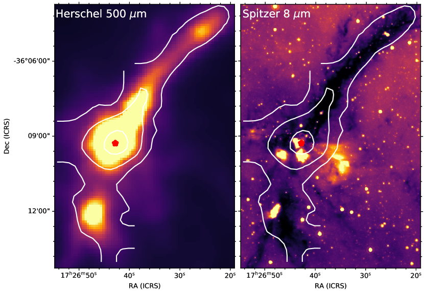
Figure 1: The map of the region G351.78–0.54 in the infrared range at $\lambda$ = 500 $\mu$m (Herschel) and 8 $\mu$m (Spitzer). The white contours show the C¹⁸O (2–1) integrated line intensity from our data. Contour levels are 5, 10, 30 K km s^-1. The position of the IR source IRAS 17233–3606 is marked with an asterisk (red).

2 Observations and data analysis

The observations were carried out with the APEX radio telescope (Güsten et al., 2006) in 2010–2017 in the wavelength ranges of 1.3 mm and 0.8 mm (projects O-085.F-9323, O-086.F-9316, O-097.F-9303, O-098.F-9306) using SHeFI receivers (Vassilev et al., 2008; Belitsky et al., 2006). The beam width at the half power level (HPBW) ranged from 27^′′ to 17^′′. The data are converted to the main beam temperature scale using the main beam efficiencies ($\eta_{mb}$) presented on the APEX web site. We adopt $\eta_{mb}=0.75$ at 1.3 mm and $\eta_{mb}=0.7$ at 0.8 mm as derived from Jupiter observations since the size of the observed compact structures is comparable to Jupiter. At 0.8 mm there is a rather large scatter in the estimates of this parameter. The adopted value is in a reasonable agreement with the most of these estimates and with the Ruze formula.

The list of the observed lines, which are analyzed here, is presented in Table 1. It includes CO (2–1), ¹³CO (2–1), C¹⁸O (2–1), ¹³CO (3–2), C¹⁸O (3–2), N₂H⁺ (3–2), CH₃CCH ($13_{K}-12_{K}$) and several HNCO transitions. The line parameters are taken mainly from the Cologne Database for Molecular Spectroscopy (CDMS) (Müller et al., 2001, 2005; Endres et al., 2016) and from the Jet Propulsion Laboratory (JPL) catalog (Pickett et al., 1998). The spectral resolution (channel width) was 244 kHz in the ¹³CO (2–1), C¹⁸O (2–1), N₂H⁺ (3–2) and HNCO observations. In the CO (2–1), ¹³CO (3–2), C¹⁸O (3–2) and CH₃CCH observations it was 76 kHz. The corresponding resolution in velocity is 0.10 km s^-1 in CO (2–1) and CH₃CCH, 0.33 km s^-1 in ¹³CO (2–1), C¹⁸O (2–1) and HNCO (10–9), 0.07 km s^-1 in ¹³CO (3–2), C¹⁸O (3–2) and HNCO (15–14), 0.26 km s^-1 in N₂H⁺ (3–2).

The median value of the RMS noise at this resolution at the $T_{\mathrm{mb}}$ scale is 0.13 K in the CO (2–1) spectra, $\sim 0.1$ K in the ¹³CO (2–1) and C¹⁸O (2–1) spectra, $\sim 0.6$ K in the ¹³CO (3–2) and C¹⁸O (3–2) spectra, $\sim 0.1$ K in the N₂H⁺ (3–2) spectra, 0.02–0.11 K in the CH₃CCH spectra, $\sim 0.07$ K in the HNCO (10–9) spectra and $\sim 0.09$ K in the HNCO (15–14) spectra.

The observations were performed in the position-switching mode. The reference positions were different for different observations. In some cases a significant emission was apparently present at the reference position resulting in negative features in the measured spectra. In particular this is a case for the ¹³CO (2–1) and C¹⁸O (2–1) observations. At least a part of these data contains a narrow such feature at –3.6 km s^-1. Its width is $\sim 0.6$ km s^-1 in C¹⁸O (2–1) and $\sim 1$ km s^-1 in ¹³CO (2–1). The integrated intensity of this feature in the average spectra is $\sim 0.3$ K km s^-1 in C¹⁸O (2–1) and $\sim 2$ K km s^-1 in ¹³CO (2–1). For C¹⁸O (2–1) it constitutes about 4% of the integrated intensity of the average spectrum and therefore has a negligible effect on the estimates of the C¹⁸O column density. However this feature should be taken into account when analyzing the line profiles. In the CO (2–1) spectra there is a negative feature at about –7 km s^-1 with the amplitude of about 2.5 K and also several features around –20 km s^-1. All these features are far from the systemic velocity of the investigated object.

The line data were processed using the CLASS program from the GILDAS (Maret et al., 2011) package, and for further analysis of the obtained images, the MIRIAD (Sault et al., 1995) and Astropy (Astropy Collaboration et al., 2018) packages were used, Starlink software package (Currie et al., 2014) was used to identify molecular clumps. Estimates of the rotational temperature for the CH₃CCH transitions were obtained with the CASSIS software. The package PySpecKit (Ginsburg & Mirocha, 2011) was used to simulate the hyperfine structure of the N₂H⁺ (3–2) line. For the excitation analysis of ¹³CO, C¹⁸O and N₂H⁺, the Radex program was used (Van der Tak et al., 2007).

Table 1: List of observed molecules

Molecule	Transition	Frequency	El
		(GHz)	(K)
CO	2–1	230.538	5.53
13CO	2–1	220.399	5.29
	3–2	330.588	15.87
C18O	2–1	219.560	5.27
	3–2	329.331	15.80
N2H+	3–2	279.512	13.41
CH3CCH	130–120	222.166	63.98
	131–121	222.163	71.18
	132–122	222.150	92.78
	133–123	222.129	128.77
	134–124	222.099	179.17
	135–125	222.061	243.97
	136–126	222.014	323.17
HNCO	100,10–90,9	219.798	47.47
	101,10–91,9	218.981	90.57
	101,9–91,8	220.585	90.92
	102,9–92,8	219.734	217.74
	102,8–92,7	219.737	217.74
	103,8–93,7	219.657	422.42
	103,7–93,6	219.657	422.42
	150,15–140,14	329.664	110.76
	152,14–142,13	329.573	281.01
	152,13–142,12	329.585	281.01
	153,13–143,12	329.460	485.67
	153,12–143,11	329.460	485.67
	154,12–144,11	329.295	761.39
	154,11–144,10	329.295	761.39

3 Results

3.1 Gas distribution and kinematics

In Fig. 2 we present maps of the integrated intensity (0th moment, M₀) in the lines ¹³CO(2–1), ¹³CO(3–2), C¹⁸O(2–1), C¹⁸O(3–2) and N₂H⁺(3–2). The filamentary structure is visible in all maps.

Fig. 3 shows the map of the integrated intensity ratio C¹⁸O(3–2)/C¹⁸O(2–1). To construct this map the C¹⁸O(3–2) map was smoothed to the same angular resolution as the C¹⁸O(2–1) map. This ratio may serve as an indicator of the physical conditions in the emission regions. The ellipses show clumps detected by GaussClump using a dense gas tracer N₂H⁺ (Sect. 3.3).

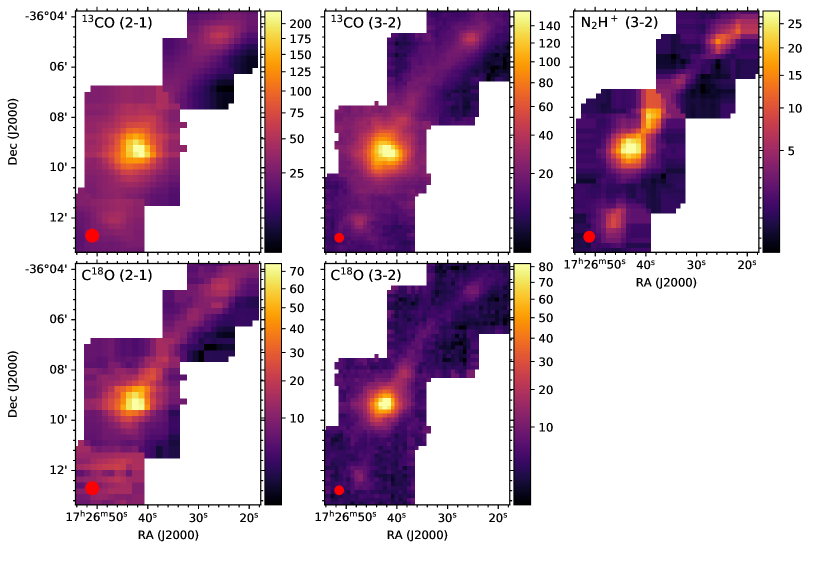
Figure 2: Integrated intensity of the lines ¹³CO (2–1), ¹³CO (3–2), C¹⁸O (2–1), C¹⁸O (3–2) and N₂H⁺ (3–2). The red circles in the lower left corners indicate the beam size (HPBW).

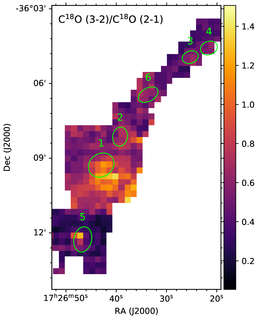
Figure 3: Integrated intensity ratio of the lines C¹⁸O (3–2)/C¹⁸O (2–1). The ellipses show clumps detected by GaussClump using the dense gas tracer N₂H⁺ (Sect. 3.3).

3.2 Column density

In order to characterize the general distribution of the CO and N₂H⁺ molecules we constructed maps of their column densities. The column densities of the C¹⁸O and N₂H⁺ molecules were calculated using the method presented in Mangum & Shirley (2015) on the basis of the C¹⁸O(2–1) and N₂H⁺(3–2) data. The first line is a tracer of the total molecular gas column density, while the second one is known to depict denser molecular gas compared to the C¹⁸O data. We assume a low optical depth in the lines and the local thermodynamic equilibrium (LTE) conditions:

$$N=\frac{3h}{8\pi^{3}S\mu^{2}}\frac{Q_{\rm rot}}{g_{J}g_{K}g_{I}}\frac{\text{exp}(\frac{E_{u}}{kT_{\rm ex}})}{\text{exp}(\frac{h\nu}{kT_{\rm ex}})-1}\frac{\int T_{\rm B}dv}{J_{\nu}(T_{\rm ex})-J_{\nu}(T_{\rm bg})},$$ (1)

$$J_{\nu}(T)=\frac{h\nu/k}{\text{exp}{\frac{h\nu}{kT}}-1},$$ (2)

where $h$ is the Planck constant, $S=J_{u}/(2J_{u}+1)$ is the line strength, $\mu$ is the dipole moment, $Q_{\rm rot}$ is the partition function, $g_{J}$ = 2J + 1 is the rotational degeneracy, $g_{K}$ is $K$-degeneracy, $g_{I}$ is the degeneracy of the nuclear spin, $J_{\nu}(T)$ is the equivalent Rayleigh-Jeans temperature, $T_{\rm ex}$ is the excitation temperature, $T_{\rm bg}$ is the background temperature and the term $\int T_{\rm R}dv$ is the integrated intensity of the line. For C¹⁸O and N₂H⁺ molecules, g_K = g_I = 1 and $Q_{\rm rot}\simeq kT/hB+1/3$, where $B$ is the rotational constant. We assume that the molecules are thermalized with the excitation temperature being equal to the gas kinetic temperature, i. e., $T_{\rm ex}=T_{\rm kin}$, and that this equals the dust temperature, $T_{\rm dust}$. We estimate the dust temperature from the Herschel Hi-GAL data at 160-–500 $\mu$m using the approach described in Mallick et al. (2015). It is based on fitting the data with a modified black body spectrum. $T_{\rm dust}$ and $N$(H₂) are free parameters. As a result, maps of the distribution of these parameters were obtained. The temperature lies in the range of 12 – 23 K, and rises towards the IRAS 17233–3606 source. However, in the direction of the IRAS source itself, it was not possible to inscribe such a model, and a temperature of 25 K was adopted there, as in Leurini et al. (2019). In general, the temperature values are very close to the map presented in (Leurini et al., 2019), so we do not show them here. Based on the 20% calibration uncertainty assigned to the Hi-GAL fluxes, a median temperature uncertainty is 13% – 18% (Battersby et al., 2011).

Assumption of $T_{\rm kin}$ = $T_{\rm dust}$ is only accurate in dense regions ($n\ga 10^{5}$ cm^-3) shielded from the UV emission, however, the gas temperature may exceed the dust temperature near infrared sources (Koumpia et al., 2015). The C¹⁸O column density is related to the hydrogen column density via a constant relative abundance C¹⁸O/H₂ = 2.0$\cdot$10^-7 (Liu et al., 2013) at the galactocentric distance of 7.4 kpc. The map of the hydrogen column density was obtained from the map of $N$(C¹⁸O) using this relation. Although the hydrogen column density was estimated also from the Hi-GAL data, we use this map for consistency with the other works (e.g Leurini et al., 2019). Next, pixel-by-pixel division of the column density maps of N₂H⁺ to H₂ was performed. The obtained maps of the distribution of the C¹⁸O, N₂H⁺ column density and N₂H⁺ relative abundance are shown in Fig. 4). On the map of the N₂H⁺ column density dense clumps are marked by white ellipses (see Sect. 3.3). It can be seen that in the direction of the luminous IR source IRAS 17233–3606, the abundance of N₂H⁺ decreases. Taking into account the uncertainties in the dust temperature and integrated intensity of the C¹⁸O and N₂H⁺ lines, we find that the $N$(C¹⁸O) uncertainty does not exceed 5% and in the direction of dense clumps with a high signal-to-noise ratio it decreases to 3%. Taking into account the negative feature in the C¹⁸O (2–1) observations caused by the emission at the reference position (Sect. 2), the column density is underestimated. Since the integrated intensity of this feature is $\sim 0.3$ K km s^-1, the corresponding column density is 1.5 $\cdot$ 10¹⁴ cm^-2, while the median $N$(C¹⁸O) is 6.7 $\cdot$ 10¹⁵ cm^-2. Hence, the average underestimation does not exceed 2%. The uncertainty in $N(\mathrm{N_{2}H^{+}})$ does not exceed 20% in the direction of dense clumps, in other directions it reaches 50%.

By integrating the column density map of hydrogen we obtain the total mass of the filament as 1800 $\pm$ 50 M_⊙. The integration area is limited by the integrated intensity of the C¹⁸O (2–1) line of 5 K km s^-1 (Fig. 1). It roughly corresponds to the signal to noise ratio of about 5 for the most noisy C¹⁸O (2–1) spectra.

The part of the filament we are studying has a length of 3.4 pc, and the mass to length ratio $M_{\rm line}$ = 529 M_⊙/pc. According to Dewangan et al. (2019), the virial (or critical) line mass for a filament with non-thermal gas motions is calculated as

$$M_{\rm line,vir}=\left[1+\left(\frac{\sigma_{\rm NT}}{c_{\rm s}}\right)^{2}\right]\times\left[16{\rm M_{\odot}pc^{-1}}\times\left(\frac{T}{10\rm K}\right)\right],$$ (3)

where $c_{\mathrm{s}}$ is the sound speed, $T$ is kinetic temperature and $\sigma_{\mathrm{NT}}$ is the non-thermal velocity dispersion, which is defined by:

$$\sigma_{\rm NT}=\sqrt{\frac{\Delta V^{2}}{8\ln 2}-\frac{kT}{30m_{H}}},$$ (4)

where $\Delta V$ is the C¹⁸O line width, $k$ is the Boltzmann constant, $m_{\rm H}$ is the mass of a hydrogen atom. The averaged over the entire filament C¹⁸O (2–1) line width is 2.5 km s^-1, the average temperature is 18 K. For our filament the critical line mass is $M_{\rm line,vir}$ = 512 M_⊙/pc. Taking into account the uncertainties, the mass to length ratio $M_{\rm line}$ is practically equal to the critical value. However, under the conditions of a possible falling motion inside the filament the velocity dispersion shows larger values than under virial equilibrium, therefore the $M_{\rm line,vir}$ artificially increases (Ballesteros-Paredes et al., 2011). Hence, the presented estimate is the upper limit of the linear critical mass. On the other hand, the derived mass to length ratio is also an upper limit since it does not take into account a possible inclination of the filament. In any case the observations show that the process of fragmentation is going on.

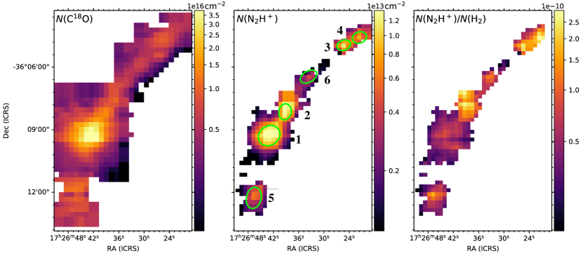
Figure 4: The column density of C¹⁸O (left), N₂H⁺ (middle), and the relative abundance of N₂H⁺ (right). The ellipses show clumps detected by GaussClump using a dense gas tracer N₂H⁺ (Sect. 3.3).

3.3 Clumps

The GaussClumps algorithm, first proposed in Stutzki & Guesten (1990), was used to identify molecular clumps. In the position-position-velocity data cube, the absolute maximum of the emission is allocated, then a three-dimensional Gaussian is fitted into the position of this maximum, which is subtracted from the original cube. After that, the next maximum is searched, followed by inscription and subtraction. This happens until the criterion for the completion of the algorithm is satisfied.

In the present work, emission of the dense gas indicator N₂H⁺(3–2) was used to identify clumps. Six clumps were found in this way, the following algorithm completion parameters were used: FWHM emission patterns in pixels (FwhmBeam) = 2.25, FWHM velocity is 3.0 km/s. Clump dimensions are defined as widths at the level of the half intensity ($\Theta_{FWHM}$). The visualization of clumps is shown in Fig. 4. The clump parameters are presented in Table 2.

We obtain the mass of the gas by integrating the $N_{\mathrm{H}_{2}}$ column density over the surface of the clump $dA$ and the virial parameter of clumps $\alpha_{\rm vir}$=M_vir/M according to the definition in Ryabukhina et al. (2018). To determine the mass of the clumps, the dust temperature obtained from the Herschel data was taken (Sect. 3.2). Integration was carried out over regions with sizes two times larger than in Fig. 4 in order to trace most of the clump emission, since the figure shows the sizes at the half intensity level. The resulting masses are presented in Table 2, where $\alpha_{2000}$ and $\delta_{2000}$ are coordinates of the center of the clump, $D$ is the clump size, FWHM (C¹⁸O) is the C¹⁸O (2–1) line width (used to determine the virial mass), $T$ is the average dust temperature according to Herschel data, $M$ is the clump mass, $M_{\rm vir}$ is the virial mass, $\alpha_{\rm vir}$ is the virial parameter.

According to Kauffmann et al. (2013), clumps are unstable and star formation processes can start when $\alpha_{\rm vir}\lesssim\alpha_{\rm crit}\simeq 2$. According to the values we obtained, this criterion is met by all clumps except the sixth one.

Spectra averaged over clumps are shown in Fig. 5. The blue dashed lines indicate the systemic velocity of each clump as $V_{\rm LSR}$ of the C¹⁸O (3–2) line. The velocity values are given in Table 2. The green solid lines indicate the velocity of the emission at the reference position in the ¹³CO and C¹⁸O (2–1) lines. Optically thick CO (2–1) line shows a complex wide spectrum with dips. The maximum width (up to 10 km/s) is observed in the direction of the first clump, and such a width may indicate outflow in this direction. The spectra of ¹³CO J = 2–1, 3–2 are narrower. The blue asymmetry of the ¹³CO (3–2) line seen in all clumps is indicative of infall (e.g. Snell & Loren, 1977). The profiles of the ¹³CO (2–1) line can be influenced by the emission at the reference position. Nevertheless, they also show real self-absorption dips at least in the first and second clumps (at about –2 km s^-1). The optically thin C¹⁸O line has an even smaller width and smaller dips, and in N₂H⁺ (3–2) toward the first clump there is no dip at all.

It is worth mentioning the apparent velocity shift between N₂H⁺ (3–2) and CO isotopologues in some clumps. We discuss this later.

According to Fig. 3, the ratio of the integrated intensities C¹⁸O(3–2)/C¹⁸O(2–1) reaches a value $\sim 1.5$ toward the first clump, however, in Fig. 5 the intensities are approximately equal. The reason is that in Fig. 5 spectra averaged over clumps are presented; therefore, the high ratio, which appears in some pixels, is smoothed out.

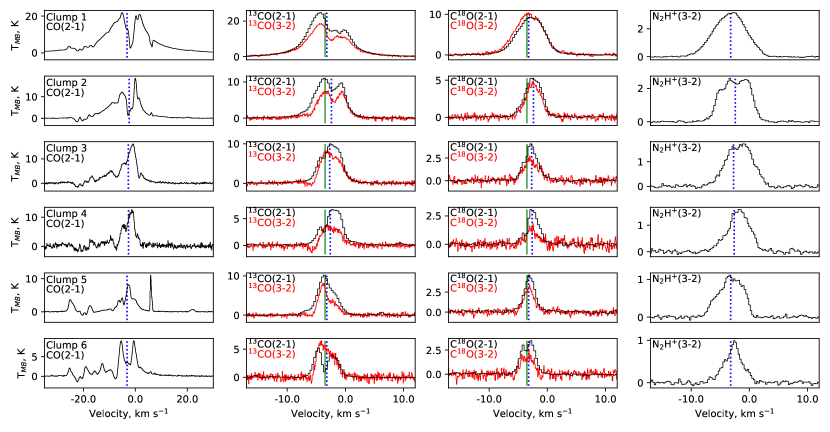
Figure 5: Spectra of lines CO (2–1), ¹³CO (2–1), ¹³CO (3–2), C¹⁸O (2–1), C¹⁸O (3–2) and N₂H⁺ (3–2) in a clumps. The dashed lines indicate LSR velocity of each clump as obtained from the C¹⁸O (3–2) line, the green solid lines indicate velocity of – 3.5 km s^-1

Table 2: Clumps parameters

Clump	$\alpha_{2000}$, h m s	$\delta_{2000}$, $\circ$ $\prime$ $\prime\prime$	D, pc	FWHM C18O (2–1), km s-1	$V_{\rm LSR}$ C18O (3–2) , km s-1	T, K Herschel	M, M⊙	Mvir, M⊙	$\alpha_{vir}$
1	17 26 43	-36 09 18	0.30 $\times$ 0.26	5.46 $\pm$ 0.04	– 3.15 $\pm$ 0.01	25	635 $\pm$ 25	889	1.4
2	17 26 39	-36 08 09	0.17 $\times$ 0.22	3.39 $\pm$ 0.03	– 2.39 $\pm$ 0.02	18	173 $\pm$ 13	235	1.35
3	17 26 25	-36 04 58	0.19 $\times$ 0.14	2.73 $\pm$ 0.05	– 2.76 $\pm$ 0.04	15	84 $\pm$ 9	130	1.55
4	17 26 21	-36 04 36	0.20 $\times$ 0.15	2.32 $\pm$ 0.06	– 2.65 $\pm$ 0.06	14	57 $\pm$ 8	100	1.75
5	17 26 46	-36 12 17	0.20 $\times$ 0.29	2.17 $\pm$ 0.04	– 3.15 $\pm$ 0.02	17	160 $\pm$ 13	121	0.76
6	17 26 33	-36 06 28	0.25 $\times$ 0.15	2.85 $\pm$ 0.07	– 3.46 $\pm$ 0.04	14	77 $\pm$ 9	166	2.15

We modelled the C¹⁸O (3-2)/(2-1) ratio with the Radex package (Fig. 6) assuming the C¹⁸O column density sufficiently low to ensure a low optical depth in the lines. By comparison with the observations this model places some constraints on the density and/or temperature of the clumps. For the first clump the observed ratio reaches a value $\sim 1.5$. This is inconsistent with the temperature of 25 K from the Herschel data (Table 2). However for the average spectra the ratio is $\sim 1$, which implies density $\sim 4\times 10^{4}$ cm^-3at $T_{k}=25$ K. For the second clump the average ratio is also $\sim 1$. At the temperature of 18 K from Herschel this implies a very high density $\ga 10^{6}$ cm^-3. However, our CH₃CCH data indicate a somewhat higher temperature (see below) which is consistent with the density similar to that in the first clump. For the other clumps the C¹⁸O (3-2)/(2-1) ratio varies from $\sim 0.5$ to $\sim 0.75$ and their temperature according to Herschel is $\sim 15$ K. This implies densities $\sim 3\times 10^{4}$ cm^-3.

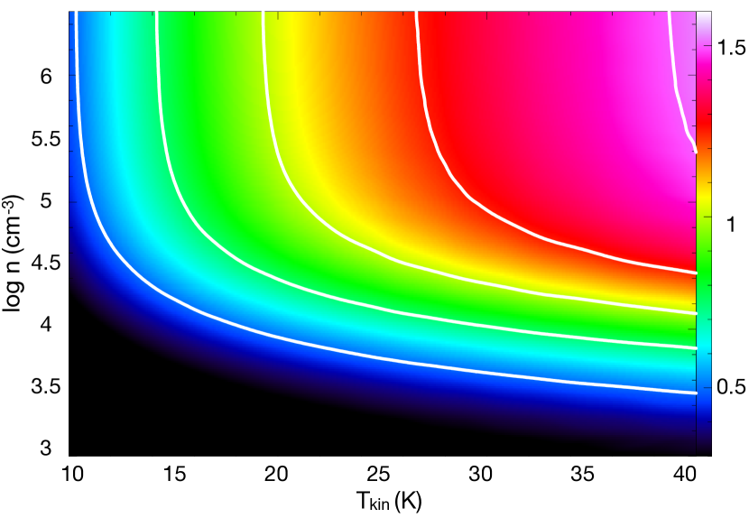
Figure 6: Model dependence of the intensity ratio of C¹⁸O (3–2)/C¹⁸O (2–1) on the gas temperature and density. White contours correspond to ratios 0.5, 0.75, 1.0, 1.25, 1.5.

In order to better characterize kinematics of the clumps we present in Fig. 7 maps of the first moment (which correspond to the velocity) and the line width (obtained from fitting by a single Gaussian) in the N₂H⁺(3–2) line toward all six clumps. In most clumps there are apparent velocity gradients. The line width peaks in the center of the clumps. We discuss these maps in Sect. 4.

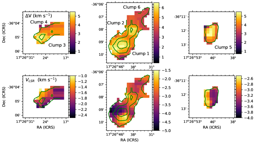
Figure 7: Maps of the first moment (bottom) and line width (top) in the N₂H⁺ (3–2) line toward various clumps. Green contours show the integrated intensity of the N₂H⁺ line, the levels are at 3, 10, 20 K km s^-1

Fig. 8 shows the map of the region G351.78–0.54 in the mid-infrared range at $\lambda$ = 24 $\mu$m (Spitzer) with clumps, obtained in this work. There is a chain of mid-IR sources along the filament, but in clumps 1–3 and 5 they are the most luminous.

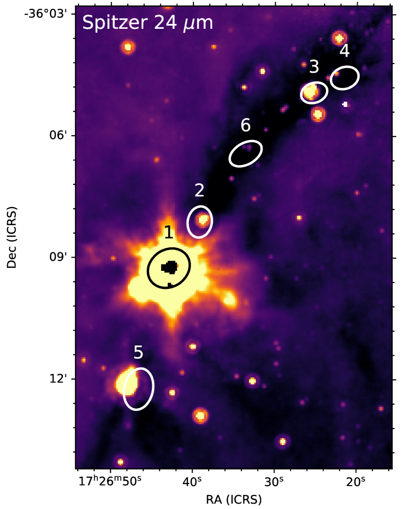
Figure 8: The map of the region G351.78–0.54 in the infrared range at $\lambda$ = 24 $\mu$m (Spitzer). Ellipses show clumps detected by GaussClump using a dense gas tracer N₂H⁺

3.4 Kinetic temperature from CH₃CCH

The kinetic temperature of the gas was estimated from observations of the CH₃CCH (13–12) line using the “rotation diagram" or “population diagram" method (Goldsmith & Langer, 1999). The methylacetylene molecule is a type of symmetric top and is a reliable indicator of kinetic temperature even at rather low densities (Bergin et al., 1994). These calculations were performed using the Cassis program. For several lines of the same rotational transition with different values of the $K$ projection for a molecule of the symmetric top type, under the LTE conditions the following relation holds:

$$\ln\frac{N_{\rm u}}{g_{\rm u}}=\ln\frac{N_{\rm tot}}{Q(T_{\rm rot})}-\frac{E_{\rm U}}{kT_{\rm rot}},$$

where $N_{\mathrm{u}}$ is the population of each level, $g_{u}$ is statistical weight, $N_{\mathrm{tot}}$ is total column density. Up to 7 lines of the CH₃CCH (13–12) transition are detected (see Table 1), for which we build the dependence of $\ln\frac{N_{\mathrm{u}}}{g_{\mathrm{u}}}$ on $\frac{E_{\rm U}}{k}$. The kinetic temperature $T$ is found as the reciprocal of the slope of a straight line approximated by this dependence. A total of six positions were observed along the filament, however, a sufficiently strong emission is detected only toward the first and second clumps. An example of the $\ln\frac{N_{\mathrm{u}}}{g_{\mathrm{u}}}$ dependence for the first spectrum in the IRAS 17233–3606 direction is shown in the Fig. 9. In this direction, 7 CH₃CCH (13–12) lines are detected (Fig. 10), however, the first two lines J = 13₀ – 12₀ and 13₁ – 12₁ are blended and it is impossible to reliably determine the integrated intensities for them. The temperature derived from the higher excitation lines from 13₃–12₃ to 13₆–12₆ is 119.7 $\pm$ 2.1 K. In the direction of the second clump, lines from 13₀–12₀ to 13₃–12₃ are observed, and the temperature according to the rotation diagram is 26 $\pm$ 4.5 K.

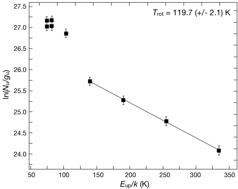
Figure 9: The rotation diagram for the CH₃CCH transitions detected toward IRAS 17233–3606

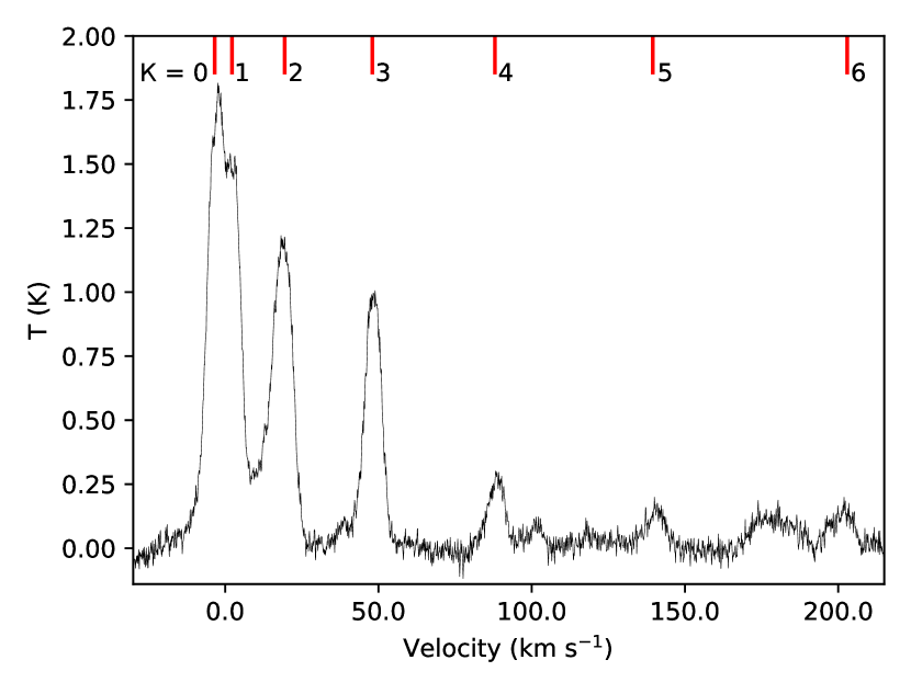
Figure 10: The CH₃CCH spectrum toward IRAS 17233–3606

3.5 HNCO toward IRAS 17233–3606

HNCO is a valuable probe of high mass star-forming regions (Zinchenko et al., 2000). Our data set includes several HNCO lines, which belong to the $J=10-9$ and $J=15-14$ transitions with the excitation energies up to $\sim 800$ K above the ground level (Table 1). The HNCO emission is detected exclusively toward the IR source IRAS 17233–3606. Examples of the detected lines are given in Fig. 11. The size of the emission region in the $J_{K_{-1}}=10_{0}-9_{0}$ line is comparable to the beam size. A 2D Gaussian fit gives the size $\approx 41^{\prime\prime}\times 34^{\prime\prime}$. Leurini et al. (2011a) measured with the Submillimeter Array (SMA) the deconvolved size in this line $2\aas@@fstack{\prime\prime}5\times 2\aas@@fstack{\prime\prime}1$. The emission in the $J_{K_{-1}}=10_{3}-9_{3}$ lines was point-like with their beam ($5\aas@@fstack{\prime\prime}4\times 1\aas@@fstack{\prime\prime}9$). A comparison of our HNCO line intensities with those measured by Leurini et al. (2011a) shows a significant flux loss (by a factor of 3) in the $J_{K_{-1}}=10_{0}-9_{0}$ line observations with the SMA. At the same time there is no flux loss for the $J_{K_{-1}}=10_{3}-9_{3}$ line. It shows that the emission in the latter line is really point-like while the $J_{K_{-1}}=10_{0}-9_{0}$ emission contains an extended component resolved out with the SMA.

Figure 11: Examples of the HNCO $J=15-14$ spectra measured toward IRAS 17233–3606. No baseline correction was applied. The spectra are shifted along the ordinate axis for clarity.

The $J_{K_{-1}}=10_{0}-9_{0}$ and $J_{K_{-1}}=15_{0}-14_{0}$ emission spectra show broad wings, which most probably arise in the outflow. It is known that HNCO is an outflow tracer (Zinchenko et al., 2000). The orientation of the HNCO outflow is in a good agreement with the observations of the outflowing gas in the lines of other molecules (Leurini et al., 2008; Klaassen et al., 2015).

The rotation diagram for the HNCO lines detected toward IRAS 17233–3606 is presented in Fig. 12. The $J=15-14$ transitions are well fitted by a single component with the rotational temperature of $T_{rot}=297\pm 8$ K. The excitation energy of the upper levels of these transitions exceeds 100 K. The $J=10-9$ transitions with lower excitation temperatures clearly indicate a lower rotational temperature. However its a more or less reliable estimate from these data looks difficult. A rough value is between 50 and 100 K. The point corresponding to the $J_{K_{-1}}=10_{3}-9_{3}$ transitions with the excitation energy of the upper level about 430 K lies somewhat lower than the fit to the $J=15-14$ data. This can be explained by the source compactness since no correction for the beam size was applied. Taking into account the difference in the beam sizes for the $J=10-9$ and $J=15-14$ transitions, this point is in a good agreement with the least squares fit mentioned above.

Figure 12: The rotation diagram for the HNCO transitions detected toward IRAS 17233–3606. The open symbols correspond to the $J=10-9$ transitions and the filled symbols correspond to the $J=15-14$ transitions. The solid line represents a least squares fit to the $J=15-14$ data. Its slope corresponds to the rotational temperature of $T_{rot}\approx 300$ K.

An interesting feature in the HNCO data is the apparent dependence of the central velocity (as derived from Gaussian fitting) on the excitation energy of the transition (Fig. 13). This shift greatly exceeds the measurement uncertainties and cannot be explained by instrumental effects since some of the high-excitation HNCO lines are close in frequency to other strong lines in this source, in particular C¹⁸O, which are observed at a “normal" velocity. We also cannot explain this picture by a possible misidentification of the high-excitation HNCO lines. No other reasonable identification of these lines could be found. Therefore, this dependence reflects apparently the internal kinematics of the source. It is worth noting that Leurini et al. (2011a) also measured a significant difference in the velocities of the $J_{K_{-1}}=10_{3}-9_{3}$ and $10_{0}-9_{0}$ transitions in the same sense as in our data. This dependence makes the rotational diagram analysis questionable, since the emission in different transitions comes apparently from different regions. At the same time the widths of the higher excitation HNCO lines ($E_{u}\ga 200$ K) do not show any dependence on the excitation energy, while the lower excitation lines are somewhat broader (Fig. 14). These broader line widths include apparently the contribution from the line wings arising in the outflow.

Figure 13: The LSR velocities measured in the HNCO lines detected toward IRAS 17233–3606 in dependence on the excitation energy of the upper level. The symbols are the same as in Fig. 12.

Figure 14: Widths the HNCO lines detected toward IRAS 17233–3606 in dependence on the excitation energy of the upper level. The symbols are the same as in Fig. 12.

4 Discussion

In Leurini et al. (2011b), a search for clumps by the ClumpFind method was also performed in the maps of the 870 $\mu$m continuum and their parameters were found. The position of our first clump corresponds to the first clump from Leurini et al. (2011b), the second corresponds to the second, third to fifth, fourth to sixth, fifth to third, sixth to seventh. The numbering of our clumps is based on the intensity of the emission peak, which decreases with increasing the number. The clumps we found are relatively large (for example, 43” $\times$ 38” in Leurini et al. (2011b) and 64” $\times$ 54” for our first clump). The intensities and profiles of the ¹³CO (2–1) and C¹⁸O (2–1) lines presented here and in Leurini et al. (2011b) are similar in general. Some differences can be related to the fact that we present spectra averaged over the clumps, while in Leurini et al. (2011b) spectra at single positions are given. In addition, the spectra, especially ¹³CO (2–1) can be influenced by the emission at the reference position (Sect. 2).

The filament contains sources at different stages of evolution. The central source IRAS 17233–3606 is considered the most evolved and probably represents a region of massive star formation (Yu et al., 2018). Three protostellar objects (AGAL351.774-00.537, 351.784-00.514, 351.804-00.449) are distributed along the filament. AGAL351.774-00.537 corresponds to the first clump, AGAL351.784-00.514 corresponds to the second clump, AGAL351.804-00.449 corresponds to the third clump. In the southern part of the filament there is a region of ionized hydrogen AGAL351.744-00.577, which is associated with our fifth clump (Contreras et al., 2013). It is worth noting that all our clumps are associated with the mid-IR sources (Fig. 8), which confirms their protostellar nature.

In our analysis the main filamentary body has a mass of $\sim 1800$ M_⊙. This value is somewhat higher than obtained by Leurini et al. (2019) using dust temperature from Herschel and C¹⁸O (2–1) molecular data ($\sim 1200$ M_⊙). However, the estimate of the filament mass from the dust emission using the Hi-GAL column density map is $\sim$ 1870 M_⊙ disregarding the region near the first clump, which is $\sim$ 190 M_⊙ (Leurini et al., 2019). Our filament mass is closer to the latter value. As shown in Sect. 3.2 the mass to length ratio $M_{line}$ is practically equal to the critical value, although both values represent upper limits. Nevertheless, the presence of several dense clumps along the filament shows that the process of fragmentation is going on.

The average clump densities estimated from the $J=2-1$ and $J=3-2$ C¹⁸O line intensity ratio are $\sim(3-4)\times 10^{4}$ cm^-3 (Sect. 3.3). Another estimate can be obtained from comparison of our N₂H⁺(3–2) data with the N₂H⁺ (1–0) observations in Leurini et al. (2011b).

In Leurini et al. (2011b) spectra of the N₂H⁺ (1–0) are presented in the direction of the first, second and fifth clumps (which correspond to our first, second and third one). In the first clump, the spectrum has the antenna temperature $\sim$ 2 K, and very broad lines: 7 hyperfine components merge into 2, and in the direction of the second and fifth clumps, the temperature is 1.4 and 1.2 K, respectively, and the lines merge into three. According to the MALT90 survey Rathborne et al. (2016), the N₂H⁺ (1–0) antenna temperature of the first clump is 2.2 $\pm$ 0.04 K, the line width is 5.03 $\pm$ 0.08 km/s. This width was obtained by approximating the line with three Gaussian functions. The N₂H⁺ (3–2) line splits into 38 hyperfine components closely spaced in frequency (Pagani et al., 2009). Due to turbulent line broadening, the components merge into one. We fit the observed profiles by a set of these components assuming a low optical depth in the line and equal excitation temperatures for all of them. For example, for the first clump, the line can be approximated by a single Gaussian function with an amplitude of 2.23 $\pm$ 0.01 K and a line width of 6.5 $\pm$ 0.03 km s^-1, but the multi-component fit gives the line width of 6.33 $\pm$ 0.02 km s^-1, and the intensity of the brightest component of 0.401 $\pm$ 0.001 K. The parameters of the hyperfine structure of the N₂H⁺ (3–2) line for the all clumps are shown in Table 3, where $T$ is the maximum intensity for the $F_{1}F=4,5-3,4$ transition at $\nu$ = 279511.8577 MHz. This estimate takes into account the convolution of the map with the same beam width as in Leurini et al. (2011b) (35^′′). For the N₂H⁺ (1–0) line, the overlap is not so high, only three central components overlap. Modeling shows that for the first clump, the overlap of three components with a line width of 4.55 km/s (Leurini et al., 2011b) and a maximum intensity of the central component ($F_{1}F=2,3-1,2$) of 1.1 K gives an observed intensity of 2.2 K. For the second clump with a line width is 3.06 km/s a maximum intensity of the most intense component is 0.7 K, for the third clump it is 0.6 K. This analysis shows that the linewidth of N₂H⁺ $J=3-2$ line is higher than $J=1-0$. It is likely that in the $J=3-2$ line we see a denser gas with a higher turbulence.

Leurini et al. (2011b) determined the N₂H⁺ column density for the first clump 5.5–10.3 $\times 10^{13}$ cm^-2, for the second clump 2.5 $\times 10^{13}$ cm^-2 and for the fifth clump 1.8 $\times$ 10¹³ cm^-2, in our analysis under the LTE assumption the column density of the first clump is 1.7 $\times$ 10¹³ cm^-2, for the second clump it is 1.4 $\times$ 10¹³ cm^-2, and for the third clump it is 1.1 $\times$ 10¹³ cm^-2. A non-LTE analysis using the RADEX software of the N₂H⁺ $J=1-0$ and $J=3-2$ data shows that for the first clump the hydrogen density $n({\mathrm{H_{2}}})\sim 3\times 10^{5}$ cm^-3 at the gas kinetic temperature $T_{\rm kin}\sim 30-100$ K with the column density $N(\mathrm{N_{2}H^{+}})\approx 2-3\times 10^{13}$ cm^-2, the model and observational data achieve the best agreement at $T_{\rm kin}\sim 40-50$ K and $N(\mathrm{N_{2}H^{+}})\approx 2.5\times 10^{13}$ cm^-2. For the second and the third clumps $n({\mathrm{H_{2}}})\sim 5\times 10^{5}$ cm^-3 at $T_{\rm kin}\sim 15-30$ K with the averaged value of the column density of $N(\mathrm{N_{2}H^{+}})\approx 2\times 10^{13}$ cm^-2 for the second clump and $N(\mathrm{N_{2}H^{+}})\approx 10^{13}$ cm^-2 for the third clump.

Table 3: Derived parameters of the hyperfine structure of the N₂H⁺ (3–2) line for the different clumps

Clump	$T(F_{1}F=4,5-3,4)$	$\Delta V$
	(K)	(km s-1)
1	0.401 $\pm$ 0.001	6.33 $\pm$ 0.02
2	0.361 $\pm$ 0.002	5.65 $\pm$ 0.03
3	0.219 $\pm$ 0.002	5.16 $\pm$ 0.06
4	0.196 $\pm$ 0.003	4.12 $\pm$ 0.07
5	0.149 $\pm$ 0.001	4.92 $\pm$ 0.05
6	0.117 $\pm$ 0.002	3.47 $\pm$ 0.05

The HNCO data imply even higher densities in the first clump. As shown in Zinchenko et al. (2000) the $K_{-1}=0$ transitions can be excited by collisions at densities $n\ga 10^{6}$ cm^-3. A collisional excitation of the $K_{-1}>0$ transitions requires very high densities. Most probably they are excited by Far-IR radiation, but densities in the emission regions should still be quite high. The emission in these transitions should arise in the close vicinity of the luminous IR source IRAS 17233–3606, which is consistent with the observed compactness of this emission. This clump was a target for many studies as mentioned above. We see there a range of temperatures from $\sim 25$ K derived from the Herschel data to $\sim 300$ K from our HNCO data. Apparently, this reflects the fact that it contains a hot core surrounded by a much colder extended envelope. The shift of the high-excitation HNCO lines in velocity relative to the lower excitation lines cannot be explained in a spherically-symmetric or cylindrically-symmetric optically thin case. One possibility is to abandon the assumption of a low optical depth in the high-excitation HNCO lines. In this case we can try to attribute the velocity shift to a self-absorption in infalling outer layers of the hot core. However, the spectra presented in Fig. 11 do not show signs of self-absorption and a high optical depth in so highly excited lines seems unrealistic and has never been observed in similar objects (Zinchenko et al., 2000). Another possibility is to assume an asymmetric distribution of the high-excitation HNCO molecules. In this case the shift can be attributed to orbital or radial motions. It is worth noting that Beuther et al. (2017) observed the blue-shifted absorption in the CH₃CN high-excitation transitions at about the same velocities as the high-excitation HNCO lines in our data. They attribute this shift to a contribution from the outflow. In this picture we have to assume that the high-excitation HNCO emission arises exclusively in the blue-shifted outflow lobe and is absent at the systemic velocity. Such assumption is rather strange and unusual. A more natural explanation is a movement of the hot dense core relative the surrounding medium at a velocity of a few km s^-1 along the line of sight. Such supersonic movements of young massive stars are frequently suggested to explain the morphology of UC H ii regions (e.g. Wood & Churchwell, 1989). Relative movements of a dense and more diffuse molecular gas have been reported, too, although at lower velocities (e.g. Kirsanova et al., 2008; Henshaw et al., 2013). In principle such a movement hints at the scenario of a triggered star formation under the influence of an external factor, such as an expanding shell or cloud collision.

As noticed in Sect. 3.3 there is a velocity shift between N₂H⁺ (3–2) and CO isotopologues in some clumps. Is is especially prominent in the third and forth clumps but is also noticeable in the sixth clump. Fig. 15 shows this shift in the third clump very clearly. The difference in the velocities is $\sim 1$ km s^-1. A very similar picture is observed in the forth clump. This shift is consistent with such scenario, too. Leurini et al. (2011b) suggested that an external agent might be the cause of the line broadening along the filament. The velocity shifts observed in our data support this suggestion.

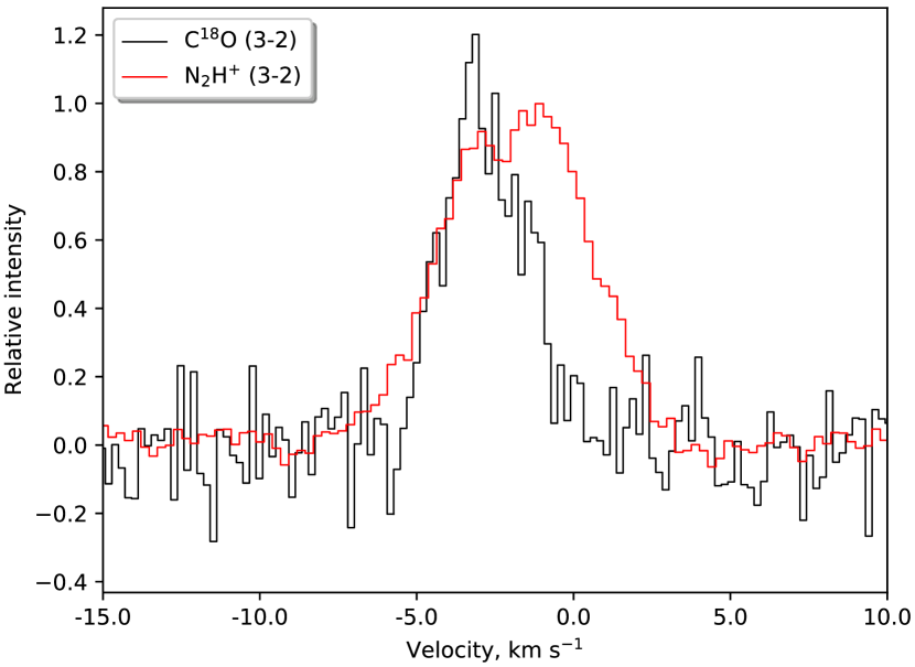
Figure 15: An overlay of the C¹⁸O (3-2) and N₂H⁺ (3–2) spectra toward the third clump. The normalized intensities of the lines are used.

Widths of all observed lines are highly supersonic. The N₂H⁺ (3–2) line width is 1.2–2.1 times higher than the C¹⁸O line width in all clumps and than the N₂H⁺ (1–0) line width in the clumps where it was observed. This hardly can be explained by the optical depth broadening (e.g. Phillips et al., 1979) since the brightness of the N₂H⁺ (3–2) line and our modeling do not support an assumption of a high optical depth. Taking into account the fact that the critical density of the N₂H⁺ (3–2) transition is much higher than critical density of the other transitions considered here, we can conclude that the velocity dispersion increases in the central denser regions of the clumps. This increase hardly can be attributed to turbulence since most clumps lack powerful sources in their interiors. Most probably the line widths increase due to Keplerian-like rotation and/or infall motions in the clumps. As mentioned above the clumps are associated with mid-IR sources, which indicates their protostellar nature. The maps of the first moment in the N₂H⁺ (3–2) line (Fig. 7) show velocity gradients in the clumps which can indicate a rotation. In the first clump the gradient is similar to that observed at small scales (Klaassen et al., 2015), which was interpreted as an evidence for rotation. The sharp increase of the line width in the center of the clumps is consistent with Keplerian-like rotation, too. However, a rotation may be not a unique interpretation of the velocity gradients in some cases. In the northern part where we see a significant difference between the velocities of N₂H⁺ (3–2) and CO isotopologues, the observed gradient can probably arise under the influence of an external factor. High resolution observations are needed to clarify kinematics of this area.

The N₂H⁺ abundance is close to the typical values (e.g. Pirogov et al., 2003). Fig. 4 shows N₂H⁺ depletion in the direction of the first clump, which contains the luminous IR source. Such behavior is rather typical for massive cores and can be probably explained by the dissociative recombination of N₂H⁺ (Pirogov et al., 2007; Zinchenko et al., 2009).

5 Conclusions

We performed a multi-line study of the filamentary infrared dark cloud G351.78–0.54 with the APEX radio telescope. The observed lines include CO (2–1), ¹³CO (2–1), C¹⁸O (2–1), ¹³CO (3–2), C¹⁸O (3–2), N₂H⁺ (3–2), CH₃CCH ($13_{K}-12_{K}$) and several HNCO transitions. The main results are the following:

1. The main filamentary body was mapped in the CO (2–1), ¹³CO (2–1), C¹⁸O (2–1), ¹³CO (3–2), C¹⁸O (3–2) and N₂H⁺ (3–2) lines. Maps of the C¹⁸O and N₂H⁺ column densities have been constructed in the LTE approximation. The total mass of the filament is estimated at $\sim 1800$ M☉. The mass per unit length ($M_{\rm line}$ = 529 M_⊙/pc) is close to the critical value. However, both values represent upper limits. The presence of several dense clumps along the filament shows that the process of fragmentation is going on.

2. Six dense clumps are identified in the N₂H⁺ (3–2) map. Their masses and virial parameters have been derived from the C¹⁸O (2–1) data assuming gas temperature equal dust temperature obtained from the Herschel data. All clumps except one appear gravitationally unstable. For two clumps we obtained temperature estimates from the CH₃CCH rotation diagrams. These temperatures are somewhat higher than the dust temperatures. In the first clump which contains the luminous IR source IRAS 17233-3606, the CH₃CCH rotation temperature is about 120 K. We use the C¹⁸O (3–2)/(2–1) intensity ratio for estimation of the clump density on the basis of non-LTE modeling. The densities obtained in this way are $n\sim 3\times 10^{4}$ cm^-3. For the three clumps with the available N₂H⁺ (1–0) data (Leurini et al., 2011b) we estimate the density from the N₂H⁺ (3–2)/(1–0) intensity ratio (taking into account the hyperfine splitting of these lines). These density estimates are about an order of magnitude higher, $n\sim 3\times 10^{5}$ cm^-3, which is consistent with the fact that N₂H⁺ traces denser regions than C¹⁸O. The width of the N₂H⁺ (3–2) lines is larger than the width of the N₂H⁺ (1–0) and C¹⁸O lines, which indicates a higher velocity dispersion in the denser parts of the clumps, which is most probably related to a Keplerian-like rotation or infall motions.

3. Exclusively toward the first clump we detected several HNCO lines with the excitation energy of the upper level up to $\sim 800$ K. The emission in the $K_{-1}=0$ transitions is rather extended and the spectra show broad wings indicative of the outflow. The orientation of the outflow lobes is in a good agreement with the observations of the outflowing gas in the lines of other molecules. The HNCO data imply even higher density in this clump, $n\ga 10^{6}$ cm^-3. The rotational temperature derived from the higher excitation transitions is $\sim 300$ K. There is a shift in velocity between the higher and lower excitation transitions, which most likely hints at a movement of the hot dense core relative the surrounding medium at a velocity of a few km s^-1 along the line of sight.

4. In some clumps there is a velocity shift $\sim 1$ km s^-1 between N₂H⁺ (3–2) and CO isotopologues. It indicates a relative movement of the dense and more diffuse gas and can be caused by an external agent as suggested earlier for explanation of the general line broadening in the filament (Leurini et al., 2011b).

5. The N₂H⁺ abundance is close to the typical values in general but drops toward the luminous IR source IRAS 17233–3606 in the first clump. This behavior is consistent with other similar objects.

6 DATA AVAILABILITY

Data directly related to this publication are available by request from the corresponding author.

References

- André et al. (2010) André P., et al., 2010, A&A, 518, L102
- André et al. (2014) André P., Di Francesco J., Ward-Thompson D., Inutsuka S.-I., Pudritz R. E., Pineda J. E., 2014, Protostars and Planets VI, pp 27–51
- Antyufeyev et al. (2016) Antyufeyev O. V., Shulga V. M., Zinchenko I. I., 2016, Kinematics and Physics of Celestial Bodies, 32, 276
- Astropy Collaboration et al. (2018) Astropy Collaboration et al., 2018, AJ, 156, 123
- Ballesteros-Paredes et al. (2011) Ballesteros-Paredes J., Hartmann L. W., Vázquez-Semadeni E., Heitsch F., Zamora-Avilés M. A., 2011, MNRAS, 411, 65
- Bally et al. (1987) Bally J., Langer W. D., Stark A. A., Wilson R. W., 1987, ApJ, 312, L45
- Battersby et al. (2011) Battersby C., et al., 2011, A&A, 535, A128
- Belitsky et al. (2006) Belitsky V., et al., 2006, in Society of Photo-Optical Instrumentation Engineers (SPIE) Conference Series. p. 62750G, doi:10.1117/12.671383
- Bergin et al. (1994) Bergin E. A., Goldsmith P. F., Snell R. L., Ungerechts H., 1994, ApJ, 431, 674
- Beuther et al. (2017) Beuther H., Walsh A. J., Johnston K. G., Henning T., Kuiper R., Longmore S. N., Walmsley C. M., 2017, A&A, 603, A10
- Beuther et al. (2019) Beuther H., et al., 2019, A&A, 621, A122
- Contreras et al. (2013) Contreras Y., et al., 2013, A&A, 549, A45
- Currie et al. (2014) Currie M. J., Berry D. S., Jenness T., Gibb A. G., Bell G. S., Draper P. W., 2014, in Manset N., Forshay P., eds, Astronomical Society of the Pacific Conference Series Vol. 485, Astronomical Data Analysis Software and Systems XXIII. p. 391
- Dewangan et al. (2019) Dewangan L. K., Pirogov L. E., Ryabukhina O. L., Ojha D. K., Zinchenko I., 2019, ApJ, 877, 1
- Endres et al. (2016) Endres C. P., Schlemmer S., Schilke P., Stutzki J., Müller H. S. P., 2016, Journal of Molecular Spectroscopy, 327, 95
- Ginsburg & Mirocha (2011) Ginsburg A., Mirocha J., 2011, PySpecKit: Python Spectroscopic Toolkit (ascl:1109.001)
- Goldsmith & Langer (1999) Goldsmith P. F., Langer W. D., 1999, ApJ, 517, 209
- Güsten et al. (2006) Güsten R., Nyman L. Å., Schilke P., Menten K., Cesarsky C., Booth R., 2006, A&A, 454, L13
- Henshaw et al. (2013) Henshaw J. D., Caselli P., Fontani F., Jiménez-Serra I., Tan J. C., Hernandez A. K., 2013, MNRAS, 428, 3425
- Kauffmann & Pillai (2010) Kauffmann J., Pillai T., 2010, ApJ, 723, L7
- Kauffmann et al. (2013) Kauffmann J., Pillai T., Goldsmith P. F., 2013, ApJ, 779, 185
- Kirsanova et al. (2008) Kirsanova M. S., Sobolev A. M., Thomasson M., Wiebe D. S., Johansson L. E. B., Seleznev A. F., 2008, MNRAS, 388, 729
- Klaassen et al. (2015) Klaassen P. D., Johnston K. G., Leurini S., Zapata L. A., 2015, A&A, 575, A54
- Koumpia et al. (2015) Koumpia E., Harvey P. M., Ossenkopf V., van der Tak F. F. S., Mookerjea B., Fuente A., Kramer C., 2015, A&A, 580, A68
- Leurini et al. (2008) Leurini S., Hieret C., Thorwirth S., Wyrowski F., Schilke P., Menten K. M., Güsten R., Zapata L., 2008, A&A, 485, 167
- Leurini et al. (2011a) Leurini S., Codella C., Zapata L., Beltrán M. T., Schilke P., Cesaroni R., 2011a, A&A, 530, A12
- Leurini et al. (2011b) Leurini S., Pillai T., Stanke T., Wyrowski F., Testi L., Schuller F., Menten K. M., Thorwirth S., 2011b, A&A, 533, A85
- Leurini et al. (2014) Leurini S., et al., 2014, A&A, 564, L11
- Leurini et al. (2019) Leurini S., et al., 2019, A&A, 621, A130
- Li et al. (2016) Li G.-X., Urquhart J. S., Leurini S., Csengeri T., Wyrowski F., Menten K. M., Schuller F., 2016, A&A, 591, A5
- Liu et al. (2013) Liu T., Wu Y., Zhang H., 2013, ApJ, 775, L2
- Low et al. (1984) Low F. J., et al., 1984, ApJ, 278, L19
- Mallick et al. (2015) Mallick K. K., Ojha D. K., Tamura M., Linz H., Samal M. R., Ghosh S. K., 2015, MNRAS, 447, 2307
- Mangum & Shirley (2015) Mangum J. G., Shirley Y. L., 2015, PASP, 127, 266
- Maret et al. (2011) Maret S., Hily-Blant P., Pety J., Bardeau S., Reynier E., 2011, A&A, 526, A47
- McClure-Griffiths et al. (2006) McClure-Griffiths N. M., Dickey J. M., Gaensler B. M., Green A. J., Haverkorn M., 2006, ApJ, 652, 1339
- Motte et al. (2018) Motte F., Bontemps S., Louvet F., 2018, ARA&A, 56, 41
- Müller et al. (2001) Müller H. S. P., Thorwirth S., Roth D. A., Winnewisser G., 2001, A&A, 370, L49
- Müller et al. (2005) Müller H. S. P., Schlöder F., Stutzki J., Winnewisser G., 2005, Journal of Molecular Structure, 742, 215
- Myers (2009) Myers P. C., 2009, ApJ, 700, 1609
- Pagani et al. (2009) Pagani L., Daniel F., Dubernet M. L., 2009, A&A, 494, 719
- Phillips et al. (1979) Phillips T. G., Huggins P. J., Wannier P. G., Scoville N. Z., 1979, ApJ, 231, 720
- Pickett et al. (1998) Pickett H. M., Poynter R. L., Cohen E. A., Delitsky M. L., Pearson J. C., Müller H. S. P., 1998, J. Quant. Spectrosc. Radiative Transfer, 60, 883
- Pilbratt et al. (2010) Pilbratt G. L., et al., 2010, A&A, 518, L1
- Pirogov et al. (2003) Pirogov L., Zinchenko I., Caselli P., Johansson L. E. B., Myers P. C., 2003, A&A, 405, 639
- Pirogov et al. (2007) Pirogov L., Zinchenko I., Caselli P., Johansson L. E. B., 2007, A&A, 461, 523
- Rathborne et al. (2006) Rathborne J. M., Jackson J. M., Simon R., 2006, ApJ, 641, 389
- Rathborne et al. (2016) Rathborne J. M., et al., 2016, Publ. Astron. Soc. Australia, 33, e030
- Ryabukhina et al. (2018) Ryabukhina O. L., Zinchenko I. I., Samal M. R., Zemlyanukha P. M., Ladeyschikov D. A., Sobolev A. M., Henkel C., Ojha D. K., 2018, Research in Astronomy and Astrophysics, 18, 095
- Sault et al. (1995) Sault R. J., Teuben P. J., Wright M. C. H., 1995, in Shaw R. A., Payne H. E., Hayes J. J. E., eds, Astronomical Society of the Pacific Conference Series Vol. 77, Astronomical Data Analysis Software and Systems IV. p. 433 (arXiv:astro-ph/0612759)
- Schisano et al. (2020) Schisano E., et al., 2020, MNRAS, 492, 5420
- Snell & Loren (1977) Snell R. L., Loren R. B., 1977, ApJ, 211, 122
- Stutzki & Guesten (1990) Stutzki J., Guesten R., 1990, ApJ, 356, 513
- Tan et al. (2014) Tan J. C., Beltrán M. T., Caselli P., Fontani F., Fuente A., Krumholz M. R., McKee C. F., Stolte A., 2014, Protostars and Planets VI, pp 149–172
- Van der Tak et al. (2007) Van der Tak F. F. S., Black J. H., Schöier F. L., Jansen D. J., van Dishoeck E. F., 2007, A&A, 468, 627
- Vassilev et al. (2008) Vassilev V., et al., 2008, A&A, 490, 1157
- Wienen et al. (2015) Wienen M., et al., 2015, A&A, 579, A91
- Wood & Churchwell (1989) Wood D. O. S., Churchwell E., 1989, ApJS, 69, 831
- Yu et al. (2018) Yu N.-P., Xu J.-L., Wang J.-J., Liu X.-L., 2018, ApJ, 865, 135
- Zinchenko et al. (2000) Zinchenko I., Henkel C., Mao R. Q., 2000, A&A, 361, 1079
- Zinchenko et al. (2009) Zinchenko I., Caselli P., Pirogov L., 2009, MNRAS, 395, 2234