From Graph Centrality to Data Depth

Abstract

Given a sample of points in a Euclidean space, we can define a notion of depth by forming a neighborhood graph and applying a notion of centrality. In the present paper, we focus on the degree, iterates of the H-index, and the coreness, which are all well-known measures of centrality. We study their behaviors when applied to a sample of points drawn i.i.d. from an underlying density and with a connectivity radius properly chosen. Equivalently, we study these notions of centrality in the context of random neighborhood graphs. We show that, in the large-sample limit and under some standard condition on the connectivity radius, the degree converges to the likelihood depth (unsurprisingly), while iterates of the H-index and the coreness converge to new notions of depth.

1 Introduction

Notions of Depth for Multivariate Distributions. In the context of multivariate analysis, a notion of depth is meant to provide an ordering of the space. While in dimension one there is a natural order (the one inherited by the usual order on the real line), in higher dimensions this is lacking, and impedes the definition of such foundational objects as a median or other quantiles, for example. By now, many notions of data depth have been proposed and the corresponding literature is quite extensive. Most of the notions are geometrical in nature, as perhaps they should be. Among these, for example, we find the half-space depth (Tukey, 1975; Donoho and Gasko, 1992), various notions of simplicial depth (Oja, 1983; Liu, 1990), or the convex hull peeling (Barnett, 1976; Eddy, 1982). Other notions of depth are not motivated by geometry, in particular the likelihood depth (Fraiman et al., 1997; Fraiman and Meloche, 1999), which is simply given by the values taken by the density (or an estimate when it is unknown). Notions of depth are surveyed in (Liu et al., 1999, 2006; Mosler, 2013).

Notions of Node Centrality for Graphs. While the focus in multivariate analysis is on point clouds, in graph and network analysis the concern is on relationships between some items represented as nodes in a graph. There, the corresponding notion is that of node centrality. (There are notions of centrality that apply to edges, but we will not consider these here.) Quite a few notions have been proposed, including the degree, the H-index (Hirsch, 2005), the coreness (Seidman, 1983), and other notions including some based on graph distances (Freeman, 1978) or on (shortest-)path counting (Freeman, 1977), and still other ones that rely on some spectral properties of the graph (Katz, 1953; Bonacich, 1972; Page et al., 1999; Kleinberg, 1999). Notions of centrality are surveyed in (Kolaczyk, 2009; Borgatti and Everett, 2006; Freeman, 1978).

From Node Centrality to Data Depth. Thus, on the one hand, notions of depth have been introduced in the context of point clouds, while on the other hand, notions of centrality have been proposed in the context of graphs and networks, and these two lines of work seem to have evolved completely separately, with no cross-pollination whatsoever, at least to our knowledge. The only place where we found a hint of that is in the discussion of Aloupis (2006), who mentions a couple of “graph-based approach[es]” which seem to have been developed for the context of point clouds, although one of them — the method of Toussaint and Foulsen (1979) based on pruning the minimum spanning tree — applies to graphs as well. We can also mention the recent work of Calder and Smart (2020), who study the large-sample limit of the convex hull peeling, relating it to a motion by (Gaussian) curvature. This lack of interaction may appear surprising, particularly in view of the important role that neighborhood graphs have played in multivariate analysis, for example, in areas like manifold learning (Tenenbaum et al., 2000; Weinberger et al., 2005; Belkin and Niyogi, 2003), topological data analysis (Wasserman, 2018; Chazal et al., 2011), and clustering (Ng et al., 2002; Arias-Castro, 2011; Maier et al., 2009; Brito et al., 1997). The consideration of neighborhood graphs has also led to the definition of geometrical quantities for graphs inspired by Euclidean or Riemannian geometry, such as the volume, the perimeter, and the conductance (Trillos et al., 2016; Arias-Castro et al., 2012; Müller and Penrose, 2020), and to the development of an entire spectral theory, in particular the study of the Laplacian (Chung, 1997; Belkin and Niyogi, 2008; Giné and Koltchinskii, 2006; Singer, 2006).

Our Contribution. Inspired by this movement, we draw a bridge between notions of depth for point clouds and notions of centrality for nodes in a graph. In a nutshell, we consider a multivariate analysis setting where the data consist of a set of points in the Euclidean space. The bridge is, as usual, a neighborhood graph built on this point set, which effectively enables the use of centrality measures, whose large sample limit we examine in a standard asymptotic framework where the number of points increases, while the connectivity radius remains fixed or converges to zero slowly enough. In so doing, we draw a correspondence between some well-known measures of centrality and depth, while some notions of centrality are found to lead to new notions of depth.

A bridge going in the other direction, namely from depth to centrality, can be built by first embedding the nodes of a graph as points in a Euclidean space, thus making depth measures applicable. We do not explore this route in the present paper.

2 Preliminaries

2.1 Depth

A measure of depth on $\mathbb{R}^{d}$ is a function ${\cal D}$ that takes a point $x$ and a probability distribution $P$, and returns a non-negative real number ${\cal D}(x;P)\geq 0$, meant to quantify how ‘significant’ $x$ is with respect to $P$. Implicit in (Liu, 1990) are a set of desirable properties that such a function ${\cal D}$ should satisfy, from which we extract the following:

• Equivariance. For any rigid transformation $\mathcal{A}:\mathbb{R}^{d}\to\mathbb{R}^{d}$,

  $${\cal D}(\mathcal{A}x;\mathcal{A}P)={\cal D}(x;P),\quad\forall\,x\in\mathbb{R}^{d}.$$ (1)

• Monotonicity. When $P$ is unimodal in the sense that it has a density $f$ that is rotationally invariant and non-increasing with respect to the origin, then for any vector $u$, $t\mapsto{\cal D}(tu;P)$ is also non-increasing on $\mathbb{R}_{+}$.

The definition of unimodality we use here is quite strict, but this is the property we are able to establish for the new notions of depth that emerge out of our study. Ideally, we would use broader definitions of unimodality — see for instance Dai (1989, Sec 3) — but it proved difficult to establish unimodality under such definitions. Incidentally, this seems to be a common difficulty when analyzing depths: see for instance the discussion in (Kleindessner and Von Luxburg, 2017, Sec 5.2) about the lens depth (Liu and Modarres, 2011).

Two measures of depth are said to be equivalent if they are increasing functions of each other, as all that really matters is the (partial) ordering on $\mathbb{R}^{d}$ that a depth function provides. Note that $P$ above may be an empirical distribution based on a sample, or an estimate of the distribution that generated that sample.

Likelihood Depth

Among the various notions of depth, the likelihood depth of Fraiman and Meloche (1999) will arise multiple times in what follows. For a distribution $P$ with density $f$, this depth is defined as ${\cal D}_{\mathrm{lik}}(x;P):=f(x)$. This is the population version, and its empirical counterpart may be defined based on an estimate of the underlying density. Note that the two conditions above, namely, equivariance and monotonicity, are trivially satisfied by the likelihood depth.

2.2 Centrality

A measure of centrality is a function ${\cal C}$ that takes a node $i\in V$ and the graph $G=(V,E)$ it belongs to, and returns a non-negative real number ${\cal C}(i;G)\geq 0$, meant to quantify how ‘central’ $i$ is in $G$. Although there does not seem to be an agreement as to what a centrality measure is (Freeman, 1978), the following properties seem desirable for a centrality measure defined on undirected, unweighted graphs:

• Invariance. The centrality is invariant under graph automorphisms (i.e., nodes re-labeling).

• Monotonicity. If we add an edge between $i$ and another node $j$, then the centrality of $i$ does not decrease.

Two measures of centrality are equivalent if they are increasing functions of each other, as again, what really matters in a measure of centrality is the ordering it induces on the nodes.

2.3 Setting and Notation

We consider a multivariate setting where

$$\mathcal{X}_{n}=\{X_{1},\dots,X_{n}\} f \mathbb{R}^{d}$$ is an i.i.d. sample from a uniformly continuous density on . (2)

Note that the dimension $d$ will remain fixed.

The bridge between point clouds and graphs is the construction of a neighborhood graph. More specifically, for an arbitrary set of distinct points, $x_{1},\dots,x_{k}\in\mathbb{R}^{d}$ and a radius $r>0$, let $\mathcal{G}_{r}(\{x_{1},\dots,x_{k}\})$ denote the graph with node set $V=\{1,\dots,k\}$ and edge set $E=\{(i,j):\|x_{i}-x_{j}\|\leq r\}$, where $\|\cdot\|$ denotes the Euclidean norm. Note that the resulting graph is undirected. Although it is customary to weigh the edges by the corresponding pairwise Euclidean distances — meaning that an edge $(i,j)$ has weight $\|x_{i}-x_{j}\|$ — we choose to focus on purely combinatorial degree-based properties of the graph, so that it is sufficient to work with the unweighted graph.

In what follows, we fix a point $x\in\mathbb{R}^{d}$ and study its centrality ${\cal C}(x;\mathcal{G}_{r}(x,\mathcal{X}_{n}))$ in the graph $\mathcal{G}_{r}(x,\mathcal{X}_{n}):=\mathcal{G}_{r}(\{x\}\cup\mathcal{X}_{n})$ as $n\to\infty$. This graph is random and sometimes called a random geometric graph (Penrose, 2003). The connectivity radius may depend on $n$ (i.e., $r=r_{n}$), although this dependency will be left implicit for the most part.

Everywhere, $\mathsf{B}(x,r)$ will denote the closed ball centered at $x$ and of radius $r$. For a measurable set $A$, $|A|$ will denote its volume. In particular, we will let $\omega$ denote the volume of the unit ball, so that $|\mathsf{B}(x,r)|=\omega r^{d}$ for all $x\in\mathbb{R}^{d}$ and $r\geq 0$. We will let

$$N:=n\omega r^{d},$$ (3)

which, as we shall see, will arise multiple times as a renormalization factor.

2.4 Contribution and Outline

We study the large-sample ($n\to\infty$) limit the centrality of $x$ in the random neighborhood graph $\mathcal{G}_{r}(x,\mathcal{X}_{n})$, where the sample $\mathcal{X}_{n}$ is generated as in (2). More specifically, we focus on the degree ${\rm deg}_{r}(x,\mathcal{X}_{n})$; on the $k$th iterate of the H-index ${\rm H}_{r}^{k}(x,\mathcal{X}_{n})$; and on the coreness ${\rm C}_{r}(x,\mathcal{X}_{n})$. As will be made clear, these notions of centrality can all be seen as iterates of the H-index, since ${\rm deg}_{r}(x,\mathcal{X}_{n})={\rm H}_{r}^{0}(x,\mathcal{X}_{n})$ and ${\rm C}_{r}(x,\mathcal{X}_{n})={\rm H}_{r}^{\infty}(x,\mathcal{X}_{n})$. Given their prominence in the literature (Malliaros et al., 2020), the degree and the coreness are examined separately. The main limits are taken as the sample size $n$ goes to infinity while the neighborhood radius $r$ remains fixed or converges to zero slowly enough. See Figure 1 for a compact summary of the main results that we derive.

Figure 1: These are the main relationships that we establish between notions of centrality and notions of depth.

Section 3 is dedicated to the degree, Section 4 to the $k$th iterate of the H-index for $1\leq k<\infty$, and Section 5 to the coreness. In Section 6 we report on some numerical simulations. The longer technical arguments are deferred to the Appendix.

3 Degree

The degree is arguably the most basic measure of centrality, and also one of the earliest to have been proposed (Freeman, 1978). In our context, the point set $\mathcal{X}_{n}$ is an i.i.d sample with common density $f$ on $\mathbb{R}^{d}$, so that it is composed of $n$ distinct points almost surely. The degree of $x\in\mathbb{R}^{d}\setminus\mathcal{X}_{n}$ in the graph $\mathcal{G}_{r}(x,\mathcal{X}_{n})$ is

$${\rm deg}_{r}(x,\mathcal{X}_{n}):=\sum_{i=1}^{n}\mathbbm{1}_{\|x-X_{i}\|\leq r}.$$ (4)

Dealing with the degree centrality is rather straightforward, but as we will consider more complex notions of centrality below, it helps to draw intuition from the continuum model where we effectively let the sample size diverge ($n\to\infty$).

Continuum degree: $r>0$ fixed

The continuous analog to the degree is naturally obtained by replacing quantities that depend on $\mathcal{X}_{n}$ by their large-sample limit, after being properly normalized. As we consider $r$-neighborhood geometric graphs, the degree of $x$ hence transforms into the convoluted density

$$f_{r}(x):=\frac{1}{|\mathsf{B}(x,r)|}\int_{\mathsf{B}(x,r)}f(z){\rm d}z.$$ (5)

More formally, we have the following well-known asymptotic behavior.

Theorem 3.1.

If $r>0$ is fixed, then almost surely,

$$\frac{1}{N}\,{\rm deg}_{r}(x,\mathcal{X}_{n})\xrightarrow[n\to\infty]{}f_{r}(x)~{}~{}\text{uniformly in $x\in\mathbb{R}^{d}$.}$$

Proof.

This comes from a direct application of Lemma A.1 to the class $\mathcal{S}_{r}=\{\mathsf{B}(x,r)~{}|~{}x\in\mathbb{R}^{d}\}$. ∎

We recover that for a neighborhood graph, the counterpart of the degree is the convoluted density $f_{r}$. This quantity, seen as a function of $P$ and $x$, clearly satisfies the requirements of a distribution depth.

Proposition 3.2.

The convoluted density $f_{r}$ satisfies the depth properties listed in Section 2.1.

Proof.

Let $x\in\mathbb{R}^{d}$ and $\mathcal{A}:\mathbb{R}^{d}\to\mathbb{R}^{d}$ be an affine isometry. The density of $\mathcal{A}P$ with respect to the Lebesgue measure is simply $f\circ\mathcal{A}^{-1}$ and

$$(f\circ\mathcal{A}^{-1})_{r}(\mathcal{A}x)=\frac{1}{\omega r^{d}}\int_{\mathsf{B}(\mathcal{A}x,r)}f(\mathcal{A}^{-1}z){\rm d}z=\frac{1}{\omega r^{d}}\int_{\mathsf{B}(x,r)}f(z){\rm d}z=f_{r}(x),$$

yielding equivariance. Monotonicity is a direct consequence of (Anderson, 1955, Thm 1). ∎

In general, when $r>0$ is fixed, the convoluted density $f_{r}(x)$ is not equivalent to the density $f$ as a measure of depth. In particular, $f_{r}(x)$ depends on $f$ in a non-local way, as it depends on the values of $f$ on $\mathsf{B}(x,r)$.

Continuum degree: $r\to 0$

Now letting $r=r_{n}$ go to zero slowly enough naturally leads us to recover the actual density.

Theorem 3.3.

If $r=r_{n}$ is such that $r\to 0$ and $nr^{d}\gg\log n$, then almost surely,

$$\frac{1}{N}\,{\rm deg}_{r}(x,\mathcal{X}_{n})\xrightarrow[n\to\infty]{}f(x)~{}~{}\text{uniformly in $x\in\mathbb{R}^{d}$.}$$

Thus, as a measure of depth, the degree is asymptotically equivalent to the likelihood depth.

Proof.

This comes from a simple application of Lemma A.1 to the collection of sets $\{\mathcal{S}_{r}\}_{r>0}$ with $\mathcal{S}_{r}:=\{\mathsf{B}(x,r)~{}|~{}x\in\mathbb{R}^{d}\}$, and of the fact that $f_{r}$ converges uniformly to $f$ since $f$ is assumed to be uniformly continuous on $\mathbb{R}^{d}$. ∎

Remark 3.4 (Kernel Density Estimator).

Defining the kernel density estimator as

$$\hat{f}(x)=\frac{1}{N}\#\{X_{i}\in\mathsf{B}(x,r)\}=\frac{1}{N}\,{\rm deg}_{r}(x,\mathcal{X}_{n}),$$ (6)

Theorem 3.3 simply restates the well-known fact that this estimator is uniformly consistent over $\mathbb{R}^{d}$ when $r\to 0$ slowly enough that $nr^{d}\to\infty$.

Remark 3.5 (Eigenvector Centrality).

Among spectral notions of centrality, PageRank is particularly famous for being at the origin of the Google search engine (Page et al., 1999). This notion of centrality was first suggested for measuring the ‘importance’ of webpages in the World Wide Web, seen as an oriented graph with nodes representing pages (URLs specifically) and a directed edge from page $i$ to page $j$ representing a hyperlink on page $i$ pointing to page $j$. For an undirected graph, like the random geometric graphs that concern us here, the method amounts to using the stationary distribution of the random walk on the graph as a measure of node centrality. This is the walk where, at a given node, we choose one of its neighbor uniformly at random. (The edge weights play no role.) However, it is well-known that the stationary distribution is proportional to the vector of degrees, so that in this particular case, PageRank as a measure of centrality is equivalent to the degree. (Again, this is not true in general for directed graphs.)

4 H-Index

4.1 H-Index

The H-index is named after Hirsch (2005), who introduced this centrality measure in the context of citation networks of scientific publications. For a given node in a graph, it is defined as the maximum integer $h$ such that the node has at least $h$ neighbors with degree at least $h$. That is, in our context, the H-index of $x$ in $\mathcal{G}_{r}(x,\mathcal{X}_{n})$ writes as

$${\rm H}_{r}(x,\mathcal{X}_{n}):=\text{largest $h$ such that }\#\big{\{}X_{i}\in\mathsf{B}(x,r):{\rm deg}_{r}(X_{i},\mathcal{X}_{n})\geq h\big{\}}\geq h.$$

The H-index was put forth as an improvement on the total number of citations as a measure of productivity, which in a citation graph corresponds to the degree. We show below that in the latent random geometric graph model of (2), the H-index can be asymptotically equivalent to the degree (see Theorems 4.2 and 4.5).

4.2 Iterated H-Index

Lü, Zhou, Zhang, and Stanley (2016) consider iterates of the mechanism that defines the H-indices as a function of the degrees: The second iterate at a given node is the maximum $h$ such that the node has at least $h$ neighbors with H-index at least $h$, and so on. More generally, given any (possibly random) bounded measurable function $\phi:\mathbb{R}^{d}\to\mathbb{R}$, we define the (random) bounded measurable function ${\rm H}_{n,r}\phi:\mathbb{R}^{d}\to\mathbb{R}$ as

$${\rm H}_{n,r}\phi(x) :=\text{largest $h$ such that }\#\big{\{}X_{i}\in\mathsf{B}(x,r):\phi(X_{i})\geq h\big{\}}\geq h$$

$$=N\max\left\{h~{}\middle|~{}\frac{1}{N}\sum_{i=1}^{n}\mathbbm{1}_{\|x-X_{i}\|\leq r}\mathbbm{1}_{\phi(X_{i})/N\geq h}\geq h\right\}.$$ (7)

The H-index ${\rm H}_{r}(x,\mathcal{X}_{n})$ can be simply written ${\rm H}_{n,r}{\rm deg}_{r}(x,\mathcal{X}_{n})$, where ${\rm deg}_{r}(x,\mathcal{X}_{n})$ was defined in the previous section. The successive iterations of the H-index ${\rm H}^{k}_{r}(x,\mathcal{X}_{n})$ are simply ${\rm H}^{k}_{n,r}{\rm deg}_{r}(x,\mathcal{X}_{n})$.

Given the variational formula (7), a natural continuous equivalent of the H-index is the ${\rm H}_{r}$ transform of the density $f$, where ${\rm H}_{r}$ is defined for any non-negative bounded measurable function $\phi:\mathbb{R}^{d}\to\mathbb{R}$ as

$${\rm H}_{r}\phi(x)=\sup\left\{t\geq 0~{}\middle|~{}\frac{1}{\omega r^{d}}\int_{\mathsf{B}(x,r)}\mathbbm{1}_{\phi(z)\geq t}f(z){\rm d}z\geq t\right\}.$$ (8)

See Figure 2 for an illustration of this transform. The $k$-th iteration of ${\rm H}_{r}$ applied to $\phi$ is simply denoted by ${\rm H}_{r}^{k}\phi$.

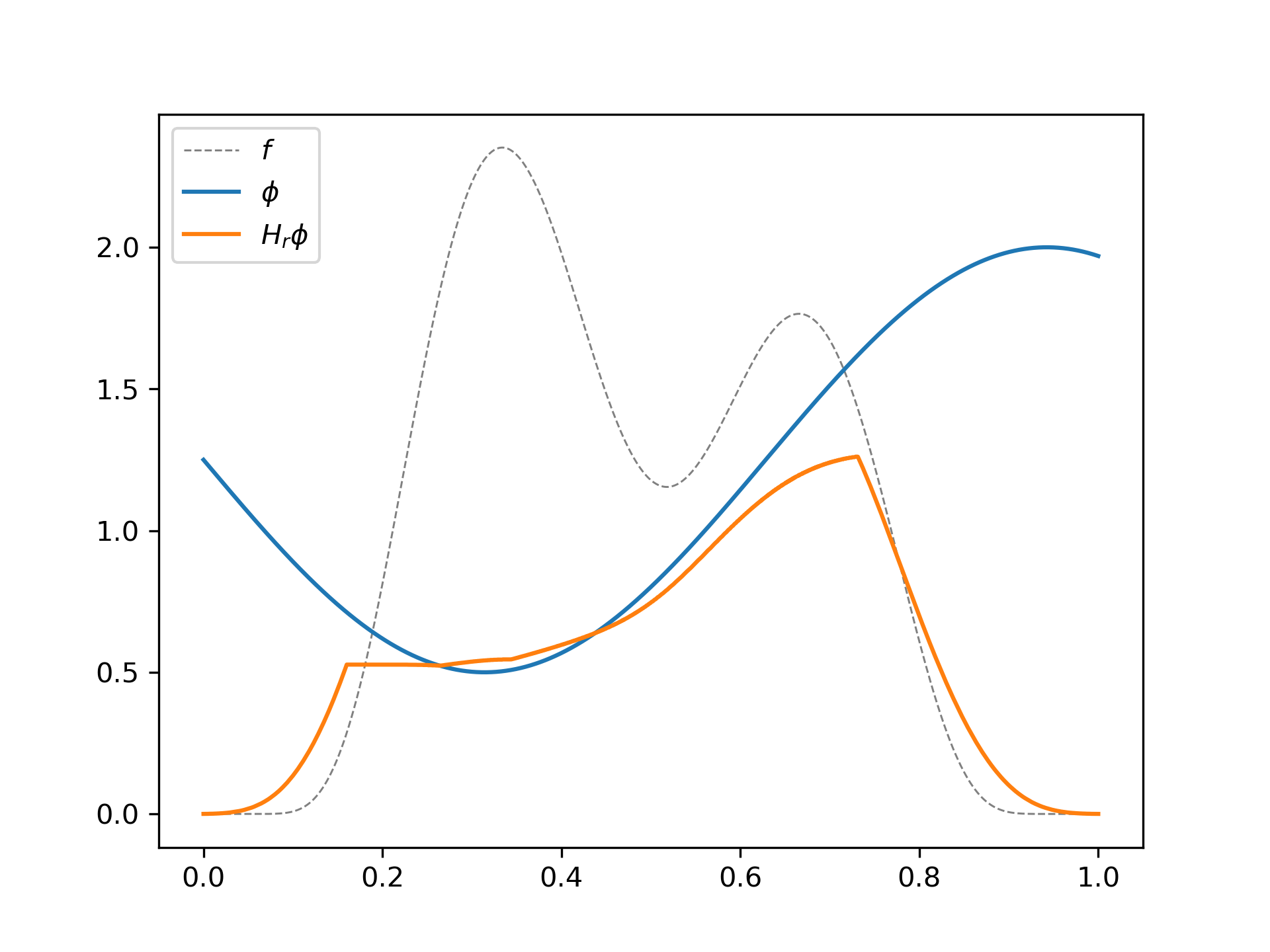
Figure 2: A density $f$, a function $\phi$, and its transform ${\rm H}_{r}\phi$ for $r=0.1$. Both $f$ and $\phi$ are smooth. ${\rm H}_{r}\phi$ does not appear to be continuously differentiable everywhere but is nonetheless Lipschitz, with Lipschitz constant no bigger than that of $f$ and $\phi$ (see Lemma B.3).

Continuum H-indices: $r>0$ fixed

As intuited above, we have the following general convergence result of the random discrete transform ${\rm H}_{n,r}$ towards the continuum one ${\rm H}_{r}$. Its proof is to be found in Section B.2.

Lemma 4.1.

Let $\phi_{n},\phi\in\ell^{\infty}(\mathbb{R}^{d})$ be random variables such that almost surely, $\frac{1}{N}\phi_{n}\xrightarrow[n\to\infty]{}\phi$ uniformly. Then almost surely, $\frac{1}{N}{\rm H}_{n,r}\phi_{n}\xrightarrow[n\to\infty]{}{\rm H}_{r}\phi$ uniformly.

When applied iteratively to the sequence of degree functions of $\mathcal{G}_{r}(x,\mathcal{X}_{n})$, Lemma 4.1 yields the following result.

Theorem 4.2.

If $r>0$ and $k\in\mathbb{N}^{*}$ are fixed, then almost-surely,

$$\frac{1}{N}\,{\rm H}^{k}_{r}(x,\mathcal{X}_{n})\xrightarrow[n\to\infty]{}{\rm H}^{k}_{r}f_{r}(x)~{}~{}\text{uniformly in $x\in\mathbb{R}^{d}$.}$$

Proof.

Apply Lemma 4.1 recursively to find that $\frac{1}{N}{\rm H}^{k}_{n,r}\phi_{n}\to{\rm H}_{r}^{k}\phi$ for all $k\geq 1$. The stated result follows readily starting from $\phi_{n}={\rm deg}_{r}(\cdot,\mathcal{X}_{n})$ and $\phi=f_{r}$. ∎

Proposition 4.3.

The $k$-iterated continuum ${\rm H}$-index ${\rm H}^{k}_{r}f_{r}$ satisfies the depth properties listed in Section 2.1.

Proof.

Equivariance is straightforward and can be shown inductively on $k\in\mathbb{N}$ using the equivariance of $f_{r}$ (Proposition 3.2).

We will now show that if $f$ and $\phi$ are rotationally invariant and decreasing with respect to the origin, then so is ${\rm H}_{r}\phi$. By induction, initializing with Proposition 3.2, this will show that ${\rm H}_{r}^{k}f_{r}$ is monotonous for all $k\in\mathbb{N}$. For any $t\geq 0$, the map $y\to\mathbbm{1}_{\phi(y)\geq t}f(y)$ is non-negative integrable and its super-level sets are centered balls, so that (Anderson, 1955, Thm 1) applies and the map

$$x\mapsto\frac{1}{\omega r^{d}}\int_{\mathsf{B}(x,r)}\mathbbm{1}_{\phi(z)\geq t}f(z){\rm d}z$$

is decreasing with respect to the origin, yielding that ${\rm H}_{r}\phi(x)\leq{\rm H}_{r}\phi(y)$ for any $x,y\in\mathbb{R}^{d}$ such that $\|x\|\geq\|y\|$. Rotational invariance of ${\rm H}_{r}\phi$ is immediate. ∎

The iterated continuum ${\rm H}$-indices ${\rm H}^{k}_{r}f_{r}$ behave very differently from the likelihood depth, as shown in Figure 3. Note also that for $k\geq 1$, ${\rm H}^{k}_{r}f_{r}(x)$ depends on $f$ in an even less local way than $f_{r}$, since it depends on the values of $f$ on $\mathsf{B}(x,(k+1)r)$.

Continuum H-indices: $r\to 0$

To gain insights on what the discrete H-indices converge to as $r=r_{n}\to 0$, let us first examine how their fixed-$r$ continuous counterparts ${\rm H}_{r}^{k}f_{r}$ behave in the same regime.

Proposition 4.4.

For all $k\geq 1$, ${\rm H}^{k}_{r}f_{r}(x)\xrightarrow[r\to 0]{}f(x)$ uniformly in $x\in\mathbb{R}^{d}$.

The proof uses elementary properties of the operator ${\rm H}_{r}$, such as its monotonicity, Lipschitzness and modulus of continuity preservation. Details are provided in Section B.1. We recall that the modulus of continuity of a function $g:\mathbb{R}^{d}\to\mathbb{R}$ is defined by $\omega_{g}(u):=\sup\left\{|g(x)-g(y)|:\|x-y\|\leq u\right\}$, for all $u\geq 0$. As in the context of (2) $f$ is assumed to be uniformly continuous, $\lim_{u\to 0}\omega_{f}(u)=0$.

Proof.

On one hand, we have ${\rm H}^{k}_{r}f_{r}(x)\leq f_{r}(x)\leq f(x)+\omega_{f}(r)$. On the other hand, notice that by definition of ${\rm H}_{r}f_{r}$, we have ${\rm H}_{r}f_{r}\geq f-\omega_{f}(r)$. Using this bound recursively together with Lemma B.3, we find that ${\rm H}^{k}_{r}f_{r}\geq f-k\omega_{f}(r)$. At the end of the day, we have proven that $\|{\rm H}_{r}^{k}f_{r}-f\|_{\infty}\leq k\omega_{f}(r)$, which concludes the proof. ∎

Coming back to the discrete H-indices, we naturally get that the $k$-th iteration of the ${\rm H}$-index converges to $f(x)$ as $r=r_{n}$ converges to $0$ slowly enough, thus coinciding with the likelihood depth.

Theorem 4.5.

If $r=r_{n}$ is such that $r\to 0$ and $nr^{d}\gg\log n$, then for all $k\in\mathbb{N}$, almost-surely,

$$\frac{1}{N}\,{\rm H}^{k}_{r}(x,\mathcal{X}_{n})\xrightarrow[n\to\infty]{}f(x)~{}~{}\text{uniformly in $x\in\mathbb{R}^{d}$.}$$

Hence, as for the degree (Section 3), we see that the iterated H-indices are asymptotically equivalent to the likelihood depth when $r\to 0$ slowly enough.

Proof.

First, decompose

$$\left|\frac{1}{N}{\rm H}^{k}_{r}(x,\mathcal{X}_{n})-f(x)\right|\leq\left|\frac{1}{N}{\rm H}^{k}_{r}(x,\mathcal{X}_{n})-{\rm H}_{r}^{k}f_{r}(x)\right|+|{\rm H}_{r}^{k}f_{r}(x)-f(x)|.$$

Proposition 4.4 asserts that the second (deterministic) term converges uniformly to zero as $r\to 0$. For the first (stochastic) one, we use expressions (7) and (8) of ${\rm H}_{n,r}$ and ${\rm H}_{r}$ respectively, and the proof of Theorem 4.2, to get that

$$\left|\frac{1}{N}{\rm H}^{k}_{r}(x,\mathcal{X}_{n})-{\rm H}_{r}^{k}f_{r}(x)\right|\leq\eta:=\sup_{S\in\mathcal{S}_{r}}\frac{1}{\omega r^{d}}|P_{n}(S)-P(S)|,$$

where $P_{n}({\rm d}z)=n^{-1}\sum_{i=1}^{n}\delta_{X_{i}}({\rm d}z)$, $P({\rm d}z)=f(z){\rm d}z$, and

$$\mathcal{S}_{r} =\Big{\{}\mathsf{B}(y,r)\cap\{\phi\geq s\}~{}|~{}y\in\mathbb{R}^{d},s\geq 0,\phi\in\{f_{r},\dots,{\rm H}_{r}^{k}f_{r}\}\Big{\}}.$$

As an intersection class of two VC classes, $\mathcal{S}_{r}$ is also VC, with dimension uniformly bounded in $r$. It is composed of sets of radii at most $r$, so that Lemma A.1 applies and yields $\eta\to 0$ almost-surely as $n\to\infty$. ∎

5 Coreness

The notion of coreness is based on the concept of core as introduced by Seidman (1983). (Seidman does not mention ‘coreness’ and only introduces cores, and we are uncertain as to the origin of the coreness.) For an integer $\ell\geq 0$, an $\ell$-core of a given graph is a maximal subgraph which has minimum degree $\ell$. To be sure, this means that any node in an $\ell$-core is neighbor to at least $\ell$ nodes in that core. In a given graph, the coreness of a node is the largest integer $\ell$ such that the node belongs to an $\ell$-core. For a recent paper focusing on the computation of the $\ell$-cores, see (Malliaros et al., 2020).

The coreness is closely related to the degree and H-index. In fact, (Lü et al., 2016, Thm 1) shows that it arises when iterating the definition of the H-index ad infinitum, when starting with the degree function. That is, in our context, we will study the random coreness

$${\rm C}_{r}(x,\mathcal{X}_{n}):={\rm H}_{r}^{\infty}(x,\mathcal{X}_{n}).$$ (9)

In particular, the coreness satisfies the following fixed-point property: The coreness of node $i$ is the maximum $\ell$ such that at least $\ell$ of its neighbors have coreness at least $\ell$. Said otherwise, it is the maximal minimal degree of a subgraph $H$ that contains $x$:

$${\rm C}_{r}(x,\mathcal{X}_{n})=\max\left\{\ell~{}\middle|~{}\text{there is a subgraph $H$ of $\mathcal{G}_{r}(x,\mathcal{X}_{n})$ with $x\in H$ and $\min_{i\in H}{\rm deg}_{H}(i)\geq\ell$}\right\}.$$ (10)

The coreness was analyzed in the context of an Erdös–Rényi–Gilbert random graph in a number of papers, for example, in (Łuczak, 1991; Janson and Luczak, 2008; Pittel et al., 1996; Riordan, 2008; Janson and Luczak, 2007), and also in the context of other graph models, for example, in (Frieze et al., 2009). We are not aware of any work that analyzes the coreness in the context of a random geometric graph.

Remark 5.1.

As the non-negative integer sequence $({\rm H}_{r}^{k}(x,\mathcal{X}_{n}))_{k\geq 0}$ is non-increasing, it becomes stationary after some index $k^{\infty}<\infty$. Said otherwise, the naive algorithm computing ${\rm H}_{r}^{\infty}(x,\mathcal{X}_{n})$ by iterating the H-index terminates after a finite number of iterations, so that bounding $k^{\infty}$ is of particular computational interest. Such a bound, depending on the geometric structure of the graph, is discussed in Section 6.3.

Continuum coreness: $r>0$ fixed

As defined above in (9), the discrete coreness is obtained by applying the H-index operator to the degree infinitely many times. Having in mind Theorem 4.2, we naturally define the notion of continuum $r$-coreness by taking the limit of the iterated continuum H-index ${\rm H}^{k}_{r}f_{r}(x)$ as the number of iteration $k$ goes to $\infty$.

Proposition 5.2.

${\rm H}^{k}_{r}f_{r}(x)$ converges uniformly in $x$ as $k\to\infty$. Its limit, denoted by ${\rm C}_{r}(x,f)$, is called the continuum $r$-coreness at $x$.

Remark 5.3.

Note that since the convergence is uniform, ${\rm C}_{r}(\cdot,f)$ is uniformly continuous and its modulus of continuity is bounded from above by $\omega_{f}$ (Lemma B.3). See Figure 3 for an illustration of the convergence of the iterations ${\rm H}^{k}_{r}f_{r}$ towards ${\rm C}_{r}(\cdot,f)$.

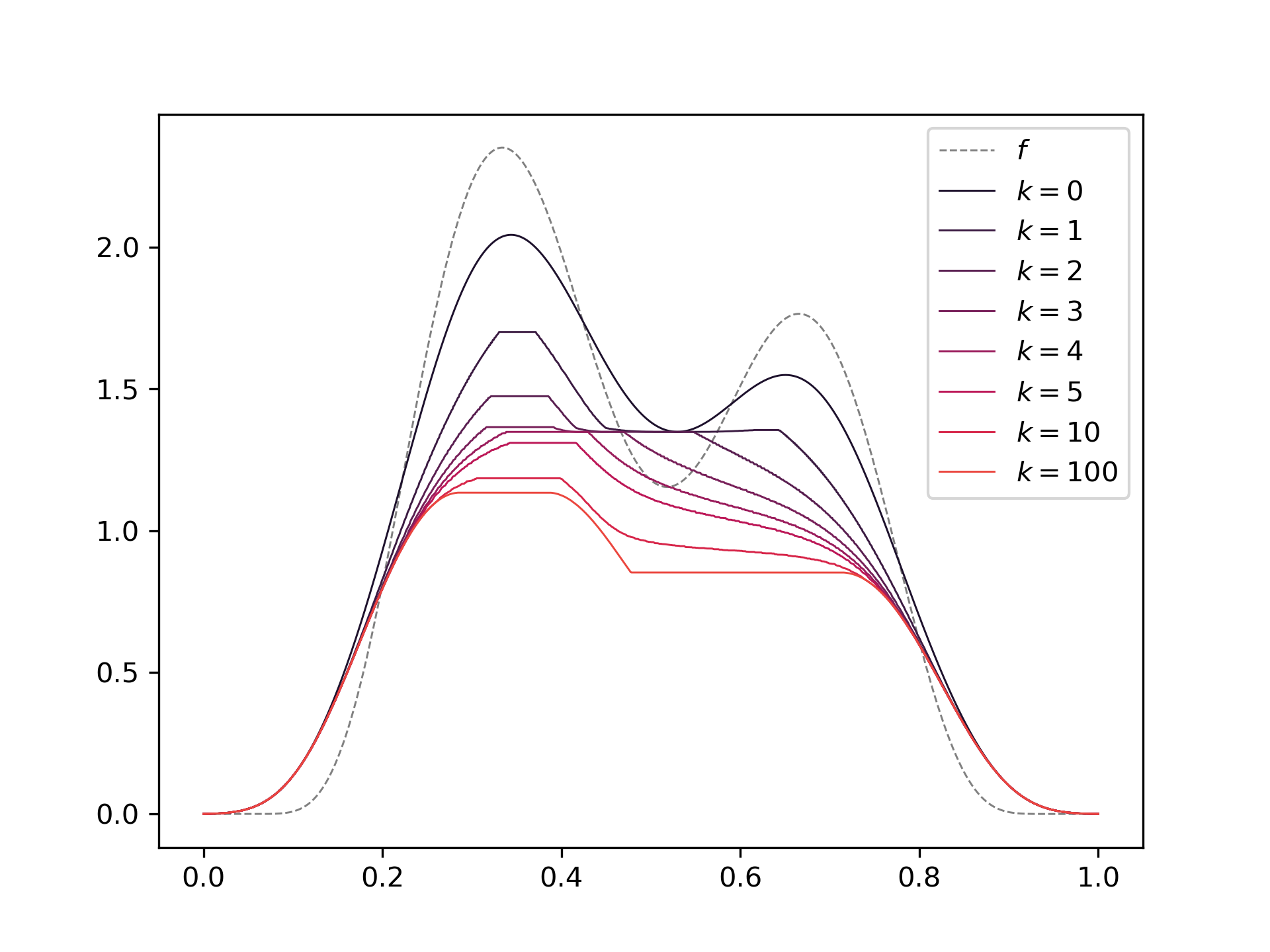
Figure 3: The successive iterations of ${\rm H}_{r}^{k}f_{r}$ (solid) for a given density $f$ (dashed), for $k$ ranging from $0$ to $100$ with $r=0.1$. The hundredth iteration is very close to its limit ${\rm C}_{r}(x,f)$.

Proof.

Since for all $t\geq 0$ and $x\in\mathbb{R}^{d}$,

$$\frac{1}{\omega r^{d}}\int_{\mathsf{B}(x,r)}\mathbbm{1}_{f_{r}(z)\geq t}f(z){\rm d}z\leq f_{r}(x),$$

so that ${\rm H}_{r}f_{r}\leq f_{r}$. Using monotonicity of the operator ${\rm H}_{r}$ (Lemma B.1) we find that $({\rm H}_{r}^{k}f_{r})_{k\in\mathbb{N}}$ is a non-increasing sequence of functions, bounded from above by $f_{r}$ and from below by $0$. In particular, it converges towards a function ${\rm C}_{r}(\cdot,f)$ pointwise. Since $|f_{r}(x)|\leq\sup_{\mathsf{B}(x,r)}|f|$ and that the latter goes to $0$ when $x$ goes to $\infty$ (since $f$ is integrable and uniformly continuous over $\mathbb{R}^{d}$), we can focus on establishing the uniform convergence of ${\rm H}_{r}^{k}f_{r}$ on a ball $\mathsf{B}(0,R)$ for an arbitrary large radius $R$. Having done so, the sequence ${\rm H}_{r}^{k}f_{r}$ is equicontinuous (from Lemma B.3), and the Arzelà–Ascoli theorem insures that the convergence towards ${\rm C}_{r}(\cdot,f)$ is uniform over $\mathsf{B}(0,R)$. ∎

By analogy with (10), we may also seek a variational characterization of ${\rm C}_{r}(x,f)$ in terms of subsets of $\mathbb{R}^{d}$, which are the natural continuous counterparts of subgraphs. This formulation, besides offering additional geometrical insights, will help with proving convergence from discrete to continuous $r$-coreness (see the proof of Theorem 5.6).

Lemma 5.4.

Let $\Omega(x)$ be the class of measurable sets $S\subset\mathbb{R}^{d}$ that contain $x$. Then for $r>0$, the continuum $r$-coreness admits the following expression

$${\rm C}_{r}(x,f)=\sup\left\{t~{}\middle|~{}\exists S\in\Omega(x)\text{ such that }\inf_{y\in S}\frac{1}{\omega r^{d}}\int_{\mathsf{B}(y,r)\cap S}f(z){\rm d}z\geq t\right\}.$$ (11)

Proof.

Let us write $F(x)$ for the supremum on the right-hand side, and show that ${\rm C}_{r}(\cdot,f)=F$ by considering their super-level sets. Let $t\geq 0$, and $S=\{F\geq t\}$. For all $y\in\mathbb{R}^{d}$, we define

$$g(y):=\frac{1}{\omega r^{d}}\int_{S\cap\mathsf{B}(y,r)}f(z){\rm d}z,$$

which, by definition of $S$, satisfies $g(y)\geq t$ for all $y\in S$. In particular, we get that for all $y\in S$,

$$\frac{1}{\omega r^{d}}\int_{\mathsf{B}(y,r)}\mathbbm{1}_{g(z)\geq t}f(z){\rm d}z\geq\frac{1}{\omega r^{d}}\int_{\mathsf{B}(y,r)}\mathbbm{1}_{z\in S}f(z){\rm d}z=g(y)\geq t,$$

so that ${\rm H}_{r}g(y)\geq t$. By induction on $k\geq 1$, we find that ${\rm H}_{r}^{k}g(y)\geq t$ for all $y\in S$, and letting $k\to\infty$, that ${\rm C}_{r}(y,f)\geq t$ for all $y\in S$, so that $S\subset\{{\rm C}_{r}(\cdot,f)\geq t\}$.

For the converse inclusion, notice that since the operator ${\rm H}_{r}$ is $1$-Lipschitz (Lemma B.2) and that ${\rm H}^{k}_{r}f_{r}$ converges uniformly towards ${\rm C}_{r}(\cdot,f)$ (Proposition 5.2), we have ${\rm H}_{r}{\rm C}_{r}(\cdot,f)={\rm C}_{r}(\cdot,f)$. Therefore, if $y\in\{{\rm C}_{r}(\cdot,f)\geq t\}$, meaning ${\rm C}_{r}(y,f)\geq t$, by definition of ${\rm H}_{r}$, we get

$$\frac{1}{\omega r^{d}}\int_{\mathsf{B}(y,r)}\mathbbm{1}_{{\rm C}_{r}(z,f)\geq t}f(z){\rm d}z\geq t$$

yielding, by maximality of $S$, that $\{{\rm C}_{r}(\cdot,f)\geq t\}\subset S$, ending the proof. ∎

Proposition 5.5.

The $r$-continuum coreness ${\rm C}_{r}(\cdot,f)$ satisfies the depth properties listed in Section 2.1.

Proof.

As ${\rm C}_{r}(\cdot,f)$ is the uniform limit (see Proposition 5.2) of functions that satisfy the properties of Section 2.1 (see Proposition 4.3), it also satisfies them. ∎

By definition, the continuum $r$-coreness ${\rm C}_{r}(\cdot,f)$ behaves roughly like ${\rm H}_{r}^{k}f_{r}$ for $k$ large enough, as shown in Figure 3. The variational formulation of Lemma 5.4 also highlights the fact that ${\rm C}_{r}(\cdot,f)$ depends on $f$ globally, as it depends on values it takes in the entire space, at least in principle. That is, perturbing $f$ very far away from $x$ may change ${\rm C}_{r}(x,f)$ drastically. In Figure 3, this phenomenon translates into the wider and wider plateaus that ${\rm H}_{r}^{k}(\cdot,f)$ exhibits as $k$ grows, which eventually approaches ${\rm C}_{r}(\cdot,f)$.

We are now in position to prove the convergence of the renormalized discrete coreness towards the $r$-continuum coreness, for a bandwidth parameter $r>0$ being fixed.

Theorem 5.6.

If $r>0$ is fixed, then almost surely,

$$\frac{1}{N}{\rm C}_{r}(x,\mathcal{X}_{n})\xrightarrow[n\to\infty]{}{\rm C}_{r}(x,f)\text{ uniformly in $x\in\mathbb{R}^{d}$. }$$ (12)

Proof.

Let $k\geq 1$. By the decreasingness of the iterations of the H-index ${\rm H}^{k}_{r}(x,\mathcal{X}_{n})$ and their convergence towards ${\rm C}_{r}(x,\mathcal{X}_{n})$ (Lü et al., 2016, Thm 1), we have that ${\rm C}_{r}(x,\mathcal{X}_{n})\leq{\rm H}^{k}_{r}(x,\mathcal{X}_{n})$. Taking $n$ to $\infty$ and using Theorem 4.2, we find that almost surely,

$$\limsup_{n\to\infty}{\rm C}_{r}(x,\mathcal{X}_{n})\leq{\rm H}^{k}_{r}f_{r}(x)$$

uniformly in $x$, so that letting $k\to\infty$ and using Proposition 5.2, we have

$$\limsup_{n\to\infty}{\rm C}_{r}(x,\mathcal{X}_{n})\leq{\rm C}_{r}(x,f).$$

For the converse inequality, we will use the variational formulation of ${\rm C}_{r}(x,f)$ given by Lemma 5.4. Let $t<{\rm C}_{r}(x,f)$ and $S\subset\mathbb{R}^{d}$ be such that $x\in S$ and

$$\frac{1}{\omega r^{d}}\int_{\mathsf{B}(y,r)\cap S}f(z){\rm d}z\geq t\quad\forall y\in S.$$

Let $H$ denote the subgraph of $\mathcal{G}_{r}(x,\mathcal{X}_{n})$ with vertices in $S$, and ${\rm deg}_{H}$ the degree of the vertices in this subgraph. We have, for all vertex $s$ in $S$,

$${\rm deg}_{H}(s)=n\times P_{n}(\mathsf{B}(s,r)\cap S)-1\geq N\times(P(\mathsf{B}(s,r)\cap S)-\eta)-1\geq N\times(t-\eta)-1,$$

where

$$\eta:=\sup_{A\in\mathcal{S}_{r}}\frac{1}{\omega r^{d}}|P_{n}(A)-P(A)|,\quad\text{with }\mathcal{S}_{r}:=\{S\cap\mathsf{B}(y,r)~{}|~{}y\in\mathbb{R}^{d}\},$$

so that ${\rm C}_{r}(x,\mathcal{X}_{n})\geq N(t-\eta)-1$. The class $\mathcal{S}_{r}$ satisfies the assumptions of Lemma A.1, and applying that lemma with $r>0$ fixed yields that, almost surely,

$$\liminf_{n\to\infty}\frac{1}{N}{\rm C}_{r}(x,\mathcal{X}_{n})\geq t$$

uniformly in $x\in\mathbb{R}^{d}$. Letting $t\nearrow{\rm C}_{r}(x,f)$ establishes

$$\liminf_{n\to\infty}\frac{1}{N}{\rm C}_{r}(x,\mathcal{X}_{n})\geq{\rm C}_{r}(x,f),$$

which concludes the proof. ∎

Continuum coreness: $r\to 0$

Seeking to complete the construction above to include asymptotic regimes where $r\to 0$, we first opt for a purely functional approach. That is, taking the limit of the continuum $r$-coreness as $r$ goes to zero.

Proposition 5.7.

${\rm C}_{r}(x,f)$ converges uniformly in $x\in\mathbb{R}^{d}$ as $r\to 0$. Its limit, denoted by ${\rm C}_{0}(x,f)$, is called the continuum coreness at $x$.

Proof.

From Lemma C.1 (proven in Section C), we get that ${\rm C}_{r}(\cdot,f)$ converges pointwise towards a limit ${\rm C}_{0}(\cdot,f)$. Since ${\rm C}_{r}(x,f)\leq f_{r}(x)\leq f(x)+\omega_{f}(r)$, and since $f\to 0$ at $\infty$ (because $f$ is integrable and is uniformly continuous), we can focus on the uniform convergence of ${\rm C}_{r}(\cdot,f)$ on a ball $\mathsf{B}(0,R)$ for some arbitrarily large $R>0$. But now, the uniform convergence on $\mathsf{B}(0,R)$ is only a consequence of the Arzelà–Ascoli theorem and the equicontinuity of ${\rm C}_{r}(\cdot,f)$ (Remark 5.3). ∎

As was shown to be the case for ${\rm C}_{r}(\cdot,f)$ in Lemma 5.4, we also give a geometric variational formulation of ${\rm C}_{0}(\cdot,f)$, which is illustrated in Figure 4.

Lemma 5.8.

Let $\Sigma(x)$ be the class of open sets $S\subset\mathbb{R}^{d}$ with smooth boundaries that contain $x$. Then the continuum coreness admits the following expression

$${\rm C}_{0}(x,f)=\sup\Big{\{}t\geq 0~{}|~{}\exists S\in\Sigma(x)\text{ such that }S\subset\{f\geq t\}\text{ and }\partial S\subset\{f\geq 2t\}\Big{\}}.$$

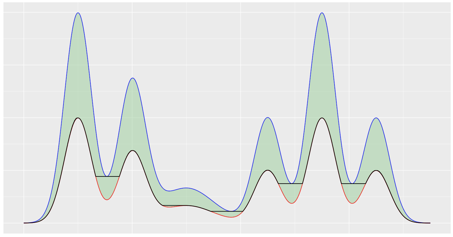
Figure 4: An illustration of $f$ (blue), $f/2$ (red) and ${\rm C}_{0}(\cdot,f)$ (black) for a mixture of $6$ Gaussians in dimension $d=1$. In the zones where ${\rm C}_{0}(\cdot,f)$ does not coincide with $f/2$, it exhibits plateaus over intervals $[x_{\min},x_{\max}]$. For $x\in(x_{\min},x_{\max})$, the supremum of Lemma 5.8 is attained for $S=(x_{\min},x_{\max})$. Otherwise, this supremum is asymptotically attained for $S=\{x\}$.

Proof sketch.

Informally, we might want to take the limit of the formulation of ${\rm C}_{r}(x,f)$ given by Lemma 5.4 as $r\to 0$: if $S\subset\mathbb{R}^{d}$ contains $x$ and is smooth (i.e., with boundary at least $\mathcal{C}^{2}$ ), then for all $y\in S$, as $r\to 0$,

$$\frac{1}{\omega r^{d}}\int_{\mathsf{B}(y,r)\cap S}f(z){\rm d}z\ \sim\ \frac{|\mathsf{B}(y,r)\cap S|}{|\mathsf{B}(y,r)|}f(y)\xrightarrow[]{}\begin{cases}f(y)&\text{if }y\in S\setminus\partial S,\\ f(y)/2&\text{if }y\in\partial S.\end{cases}$$

As a result, the requirement $\inf_{y\in S}\frac{1}{\omega r^{d}}\int_{\mathsf{B}(y,r)\cap S}f(z){\rm d}z\geq t$ becomes, roughly, $\inf_{y\in S}f(y)\geq t$ and $\inf_{y\in\partial S}f(y)\geq 2t$, which explains the given formulation of ${\rm C}_{0}(x,f)$.

See Section C for a formal proof. ∎

The above formulation clearly establishes that ${\rm C}_{0}(x,f)\leq f(x)$. On the other hand, taking for $S$ a ball centered around $x$ with an arbitrary small radius, we find that ${\rm C}_{0}(x,f)\geq f(x)/2$. The equality actually occurs whenever the homology of the super-level sets of $f$ is simple enough, as shown in Proposition 5.9. In particular, this is the case when the super-level sets are contractible sets (such as star-shaped ones), or the union of contractible sets. We defer the proof of this topological result to Section C.

Proposition 5.9.

If all the super-level sets of $f$ have a trivial $(d-1)$-th homology group over $\mathbb{Z}$, then ${\rm C}_{0}(x,f)=f(x)/2$ for all $x\in\mathbb{R}^{d}$. This is the case, for example, if $f$ is a mixture of symmetric unimodal densities with disjoint supports.

Hence, for densities $f$ with simple enough landscapes, the continuum coreness is, as a measure of depth, equivalent the likelihood depth. Otherwise, generically, ${\rm C}_{0}(\cdot,f)$ provides us with a new notion of depth that lies between $f/2$ and $f$ (see Figure 4). As is the case for ${\rm C}_{r}(\cdot,f)$, the continuum coreness ${\rm C}_{0}(\cdot,f)$ depends on the values $f$ on the entire space, at least in principle. This is apparent in the variational formulation of Lemma 5.4 and is clearly illustrated by the plateau areas of Figure 4.

Proposition 5.10.

The continuum coreness ${\rm C}_{0}(\cdot,f)$ satisfies the depth properties listed in Section 2.1.

Proof.

Let $\mathcal{A}:\mathbb{R}^{d}\to\mathbb{R}^{d}$ be an affine isometry. The density of $\mathcal{A}P$ with respect to the Lebesgue measure is given by $f_{\mathcal{A}}(x)=f(\mathcal{A}^{-1}x)$. Since $\mathcal{A}$ preserves the open sets of $\mathbb{R}^{d}$ with smooth boundaries, it follows from Lemma 5.8 that ${\rm C}_{0}(\mathcal{A}x,f_{\mathcal{A}})={\rm C}_{0}(x,f)$, so that the coreness is indeed equivariant.

If now $f$ is unimodal in the sense of Section 2.1, then its super-level sets are balls centered at the origin, and in particular they are contractible, yielding that ${\rm C}_{0}(x,f)=f(x)/2$ thanks to Proposition 5.9. The monotonicity of the coreness hence follows from that of the likelihood. ∎

We finally address the large-sample limit of ${\rm C}_{r}(x,\mathcal{X}_{n})$ as $r=r_{n}\to 0$, which does coincide with the continuum coreness ${\rm C}_{0}(x,f)$.

Theorem 5.11.

If $r=r_{n}$ is such that $r\to 0$ and $nr^{d}\gg\log n$, then almost surely,

$$\frac{1}{N}{\rm C}_{r}(x,\mathcal{X}_{n})\xrightarrow[n\to\infty]{}{\rm C}_{0}(x,f)~{}~{}\text{uniformly in $x\in\mathbb{R}^{d}$.}$$ (13)

The proof of this result, given in Section C, is fairly involved and uses an alternative definition of ${\rm C}_{0}(\cdot,f)$ that allows to control finely a stochastic term. Indeed, as one needs to handle both $r\to 0$ and $k\to\infty$ simultaneously, the VC argument used in the proofs of Theorems 4.5 and 5.6 (i.e., Lemma A.1) does not carry through.

6 Numerical Simulations

We performed some small-scale proof-of-concept computer experiments to probe into the convergences established earlier in the paper, as well as other questions of potential interest not addressed in this paper.

6.1 Illustrative Examples

In the regime where $r=r_{n}\to 0$ and $nr^{d}\gg\log(n)$, Theorems 3.3, 4.5 and 5.11 show that only $f(x)$ and ${\rm C}_{0}(x,f)$ can be obtained as limits of H-index iterates ${\rm H}_{r}^{k}(x,\mathcal{X}_{n})$, when $k\in\{0,1,\ldots,\infty\}$ is fixed. Figures 5(a) and 5(b) both illustrate, for $d=1$ and $d=2$ respectively, the following convergence behavior:

• $\frac{1}{N}{\rm deg}_{r}(x,\mathcal{X}_{n})\xrightarrow[n\to\infty]{}f(x)$ (see Theorem 3.3);

• ${\rm H}_{r}^{k}(x,\mathcal{X}_{n})\xrightarrow[k\to\infty]{}{\rm C}_{r}(x,\mathcal{X}_{n})$ (see (9));

• $\frac{1}{N}{\rm C}_{r}(x,\mathcal{X}_{n})\xrightarrow[n\to\infty]{}{\rm C}_{0}(x,f)$ (see Theorem 5.11).

The density functions have been chosen to exhibit non-trivial super-level sets, so that ${\rm C}_{0}(\cdot,f)\neq f/2$ (see Proposition 5.9).

(a) The mixture $f$ of six Gaussians in dimension $d=1$ from Figure 4 sampled $n=10000$ times. On the discrete side (solid), are displayed the degree ($k=0$), iterated H-indices for $k\in\{1,5,10,15,20\}$, and coreness $(k=\infty$). On the continuous side (dashed), the density $f$ and the continuum coreness ${\rm C}_{0}(\cdot,f)$ are plotted. Here, $r\approx 0.13$ was picked proportional to the optimal kernel bandwidth $r_{\rm opt}\asymp n^{-1/(d+2)}=n^{-1/3}$.

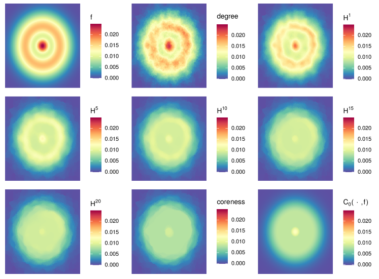
(b) A plot similar to Figure 5(a) for $d=2$. The generating density function $f$ exhibits a crater-like shape enclosing a peak, yielding a continuum coreness ${\rm C}_{0}(\cdot,f)$ that plateaus, and in particular differs from $f/2$ within the crater area. Here, $n=20000$, $k\in\{0,1,5,10,15,20,\infty\}$ and $r\asymp r_{\rm opt}\asymp n^{-1/(d+2)}=n^{-1/4}$.

Figure 5: Illustrative examples in dimension $d=1$ and in dimension $d=2$.

6.2 Convergence Rates

Intending to survey limiting properties of the degree, the H-index and the coreness, the above work does not provide convergence rates. We now discuss them numerically in the regime where $r\to 0$.

A close look at the proofs indicates that only bias terms of order $O(r\vee\omega_{f}(r))$ appear in the centrality-to-depth convergences of Theorems 3.3, 4.5 and 5.11. For the degree, the stochastic term is known to be of order $O\bigl{(}1/\sqrt{nr^{d}}\bigr{)}$. If $f$ is Lipschitz (i.e., $\omega_{f}(r)=O(r)$), the bandwidth $r_{\rm opt}$ that achieves the best minimax possible convergence rate in Theorem 3.3 is $r_{\rm opt}=O(n^{-1/(d+2)})$, yielding a pointwise error $|N^{-1}{\rm deg}_{r}(x,\mathcal{X}_{n})-f(x)|=O(r_{\rm opt})=O(n^{-1/(d+2)})$. Naturally, larger values $r\geq r_{\rm opt}$ make the bias term lead, and smaller values $r\leq r_{\rm opt}$ make the stochastic term lead. Although it remains unclear how bias terms behave for H-indices and the coreness, simulations indicate a similar bias-variance tradeoff depending on $n$ and $r$. Indeed, the sup-norms $\|N^{-1}{\rm deg}_{r}(\cdot,\mathcal{X}_{n})-f\|_{\infty}$ and $\|N^{-1}{\rm C}_{r}(\cdot,\mathcal{X}_{n})-{\rm C}_{0}(\cdot,f)\|_{\infty}$ appear to be linearly correlated (see Figure 6).

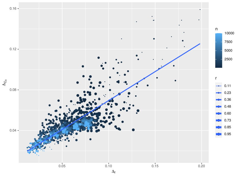
(a) Distribution of Figure 5(a) ($d=1$).

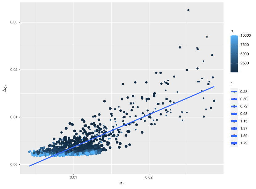
(b) Distribution of Figure 5(b) ($d=2$).

Figure 6: Scatterplot of values $\bigl{(}\|N^{-1}{\rm deg}_{r}(\cdot,\mathcal{X}_{n})-f\|_{\infty},\|N^{-1}{\rm C}_{r}(\cdot,\mathcal{X}_{n})-{\rm C}_{0}(\cdot,f)\|_{\infty}\bigr{)}$ with data generated according to (6(a)) the Gaussian mixture distribution depicted in Figure 5(a), and (6(b)) the crater-like density of Figure 5(b). Sample size values $n$ take $9$ different values in $[100,10000]$, while connection radii $r$ take $8$ different values within the interval $[0.1,0.97]$ for (6(a)) and $[0.27,1.80]$ for (6(b)). For each such pair $(n,r)$, simulations are repeated $10$ to $20$ times, depending on the value of $n$.

As a result, with a choice $r\asymp r_{\rm opt}=O(n^{-1/(d+2)})$, we anticipate

$$|N^{-1}{\rm C}_{r}(x,\mathcal{X}_{n})-{\rm C}_{0}(x)| =O(|N^{-1}{\rm deg}_{r}(x,\mathcal{X}_{n})-f(x)|)$$ (Rate Conjecture)

$$=O(n^{-1/(d+2)}),$$ (14)

with high probability. Furthermore, Figure 6 suggests that the slope relating $\|N^{-1}{\rm deg}_{r}(\cdot,\mathcal{X}_{n})-f\|_{\infty}$ and $\|N^{-1}{\rm C}_{r}(\cdot,\mathcal{X}_{n})-{\rm C}_{0}(\cdot,f)\|_{\infty}$ is of constant order, in fact between $1/2$ and $1$, which suggests very moderate constants hidden in the $O(|N^{-1}{\rm deg}_{r}(x,\mathcal{X}_{n})-f(x)|)$.

6.3 Iterations of the H-Index

Seen as the limit (9) of H-index iterations, the coreness ${\rm C}_{r}(x,\mathcal{X}_{n})={\rm H}_{r}^{\infty}(x,\mathcal{X}_{n})$ raises computational questions. One of them resides in determining whether it is reasonable to compute it naively, by iterating the H-index over the graph until stationarity at all the vertices.

More generally, given a graph $G=(V,E)$ and a vertex $v\in V$ of $G$ , and similarly as what we did in Section 4 for random geometric graphs, we can study the H-index ${\rm H}_{G}(v)$, its iterations ${\rm H}^{k}_{G}(v)$ for $k\in\mathbb{N}$, and the coreness ${\rm C}_{G}(v)$. The max-iteration $k^{\infty}(G)$ of the H-index of $G$ is then defined as the minimal number of iterations for which the iterated H-index ${\rm H}_{G}^{k}$ coincides with the coreness ${\rm C}_{G}$. That is,

$$k^{\infty}(G):=\min\big{\{}k\in\mathbb{N}~{}|~{}\forall v\in V,~{}{\rm C}_{G}(v)={\rm H}^{k}_{G}(v)\big{\}}.$$

Known bounds for $k^{\infty}(G)$ are of the form

$$k^{\infty}(G)\leq 1+\sum_{v\in V}|{\rm deg}_{G}(v)-{\rm C}_{G}(v)|~{}~{}~{}~{}\text{and}~{}~{}~{}~{}k^{\infty}(G)\leq|V|,$$

and can be found in (Montresor et al., 2013, Thm 4 & Thm 5). For random geometric graphs, this yields probabilistic bounds of order $O(n^{2}r^{d})$ and $O(n)$ respectively, with one or the other prevailing depending on whether we are in a sub-critical or super-critical regime.

However, for the random geometric graphs $\mathcal{G}(x,\mathcal{X}_{n})$, numerical simulations suggest that an even stronger bound of order $k^{\infty}(\mathcal{G}_{r}(x,\mathcal{X}_{n}))=O(nr^{d-1})$ may hold with high probability (see Figure 7). Indeed, in the regime where $r=r_{n}$ is large enough that $\mathcal{G}_{r}(x,\mathcal{X}_{n})$ is connected, this latter quantity appears to coincide with its diameter — which is of order $O(1/r)$ — multiplied by its maximal degree — which is of order $O(nr^{d})$.

Coming back to the general deterministic case, this observation leads us to conjecture that

$$k^{\infty}(G) \leq\max_{\begin{subarray}{c}H\subset G\\ \text{connected}\end{subarray}}\operatorname{diam}(H)\ \times\max_{v\in V}{\rm deg}_{G}(v),$$ (Max-Iter. Conjecture)

where $\operatorname{diam}(H)$ is the diameter of $H$ seen a combinatorial graph (with edge weight $1$). This conjecture, clearly satisfied in simulations (see Figure 7), would shed some light — if correct — on the dependency of the H-index iteration process with respect to the graph’s geometry.

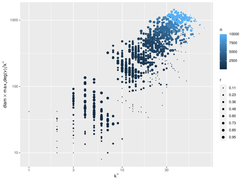
(a) Distribution of Figure 5(a) ($d=1$).

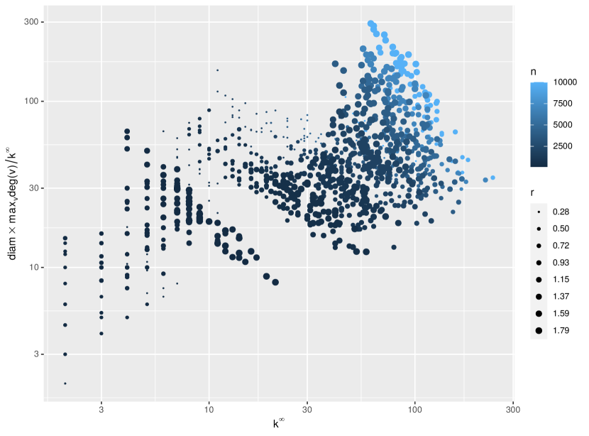
(b) Distribution of Figure 5(b) ($d=2$).

Figure 7: Scatterplot of values $\bigl{(}k^{\infty}(\mathcal{G}_{r}),\operatorname{diam}(\mathcal{G}_{r})\times\max_{v}{\rm deg}_{\mathcal{G}_{r}}(v)/k^{\infty}(\mathcal{G}_{r})\bigr{)}$ in log-log scale, with data generated according to (7(a)) the Gaussian mixture distribution of Figure 5(a), and (7(b)) the crater-like density of Figure 5(b). Values all appear to satisfy $k^{\infty}(\mathcal{G}_{r})\leq\operatorname{diam}(\mathcal{G}_{r})\times\max_{v}{\rm deg}_{\mathcal{G}_{r}}(v)$ widely (i.e., points with ordinate at least $1$ in these plots), even for small values of $r$ and $n$.

7 Concluding Remarks and Open Questions

New Notions of Depth

On the methodology side, we propose to define new notions of depth via notions of centrality applied to a properly constructed neighborhood graph — the connectivity radius playing the role of a tuning parameter. This process led us to define new notions of depth, which we called continuum H-indices and continuum coreness. We focused on the degree, the iterated H-index, and the coreness, but there are other notions of centrality, such as the closeness centrality of Freeman (1978), the betweenness of (Freeman, 1977), and other ‘spectral’ notions (Katz, 1953; Bonacich, 1972; Page et al., 1999; Kleinberg, 1999). We focused on a $r$-ball neighborhood graph construction, but there are other graphs that could play that role, such as nearest-neighbor (possibly oriented) graphs or a Delaunay triangulation. Any combination of a graph built on the sample and a centrality measure applied to the resulting graph yields a notion of data depth.

Conjectures

On the theoretic side, we obtain limits for the centrality measures that we consider. Beyond these first-order results, we could consider deriving convergence rates. In this regard, we left the conjecture displayed in (Rate Conjecture), but all the convergence rates associated with the results displayed in Figure 1 remain to be established. Another conjecture that we leave open is the bound on $k^{\infty}(G)$ displayed in (Max-Iter. Conjecture).

Appendix A A Stochastic Convergence Result

The following elementary lemma will be used throughout to control stochastic terms.

Lemma A.1.

Let $(\mathcal{S}_{r})_{r>0}$ be a family of subsets of $\mathbb{R}^{d}$ such that:

• The VC-dimension of $\mathcal{S}_{r}$ is bounded from above by some $v\in\mathbb{N}$ uniformly for all $r>0$;

• For all $r>0$ and $S\in\mathcal{S}_{r}$, we have $\operatorname{diam}(S)\leq 2r$.

Then, for any sequence $r=r_{n}$ such that $nr^{d}\gg\log n$, we have

$$\eta:=\sup_{S\in\mathcal{S}_{r}}\frac{1}{\omega r^{d}}|P_{n}(S)-P(S)|\xrightarrow[n\to\infty]{}0~{}~{}~{}\text{a.s.}$$

Proof.

We use (Anthony and Shawe-Taylor, 1993, Thm 2.1) to get that for any $r>0$ and any $\varepsilon>0$

$$\mathbb{P}\left(\sup_{S\in\mathcal{S}_{r}}\frac{1}{\sqrt{P(S)}}|P_{n}(S)-P(S)|\geq\varepsilon\right)\leq 4\Delta_{\mathcal{S}_{r}}(2n)\exp\left(-\frac{1}{4}\varepsilon^{2}n\right),$$

where $\Delta_{\mathcal{S}_{r}}(2n)$ is the scattering number of $\mathcal{S}_{r}$ on $2n$-points. Using Sauer’s lemma, we find that as soon as $2n\geq v$, we have $\Delta_{\mathcal{S}_{r}}(2n)\leq(2en/v)^{v}$. Furthermore, since $\operatorname{diam}(S)\leq 2r$ for all $S\in\mathcal{S}_{r}$, we have $\sqrt{P(S)}\leq\sqrt{\|f\|_{\infty}\omega(2r)^{d}}$ and setting $\varepsilon=\kappa\sqrt{\omega(2r)^{d}/\|f\|_{\infty}}$ yields

$$\mathbb{P}\left(\frac{1}{\omega r^{d}}\sup_{S\in\mathcal{S}_{r}}|P_{n}(S)-P(S)|\geq\kappa\right)\leq 4(2en/v)^{v}\exp\left(-\frac{1}{4\|f\|_{\infty}}\kappa^{2}n\omega(2r)^{d}\right)$$

$$\ll 4(2en/v)^{v}\exp\left(-\frac{2^{d}}{4\|f\|_{\infty}}\kappa^{2}\log n\right),$$

which yields the results when taking $\kappa$ of the form $c\log(n)^{-1/4}$ for $c$ large enough and using Borel-Cantelli lemma. ∎

Note that in particular the result is valid if $r=r_{0}$ is constant and if $\mathcal{S}_{r_{0}}$ has finite VC-dimension.

Appendix B Proofs of Section 4

B.1 Continuum H-index Properties

We start with a few elementary properties of the ${\rm H}_{r}$ transform introduced in Section 4.

Lemma B.1.

${\rm H}_{r}$ is monotonous, meaning that for any two bounded measurable functions $\phi,\psi$ on $\mathbb{R}^{d}$ such that $\phi\leq\psi$, we have ${\rm H}_{r}\phi\leq{\rm H}_{r}\psi$.

Proof.

This result is trivial once noted that the functional

$$\phi\mapsto\frac{1}{\omega r^{d}}\int_{\mathsf{B}(x,r)}\mathbbm{1}_{\phi(z)\geq t}f(z){\rm d}z$$

that appears in the definition of ${\rm H}_{r}$ is non-decreasing in $\phi$. ∎

Lemma B.2.

${\rm H}_{r}$ is $1$-Lipschitz, meaning that for any two bounded measurable functions $\phi,\psi$ on $\mathbb{R}^{d}$ we have $\|{\rm H}_{r}\phi-{\rm H}_{r}\psi\|_{\infty}\leq\|\phi-\psi\|_{\infty}$.

Proof.

Let $\varepsilon=\|\phi-\psi\|_{\infty}$. We have

$$\frac{1}{\omega r^{d}}\int_{\mathsf{B}(x,r)}\mathbbm{1}_{\phi(z)\geq t}f(z){\rm d}z\leq\frac{1}{\omega r^{d}}\int_{\mathsf{B}(x,r)}\mathbbm{1}_{\psi(z)\geq t-\varepsilon}f(z){\rm d}z$$

so that ${\rm H}_{r}\phi(x)\leq{\rm H}_{r}\psi(x)+\varepsilon$, and the proof follows. ∎

Lemma B.3.

If $\phi\in\ell^{\infty}(\mathbb{R}^{d})$ is uniformly continuous, then so is ${\rm H}_{r}\phi$ and we have $\omega_{{\rm H}_{r}\phi}\leq\omega_{\phi}\wedge\omega_{f}$. In particular, since $\omega_{f_{r}}\leq\omega_{f}$, we have $\omega_{{\rm H}_{r}^{k}f_{r}}\leq\omega_{f}$ for all $k\geq 1$.

Proof.

Let $x,y\in\mathbb{R}^{d}$, and denote $u=y-x$ and $\varepsilon=\omega_{f}\vee\omega_{\phi}(\|x-y\|)$. We have

$$\frac{1}{\omega r^{d}}\int_{\mathsf{B}(x,r)}\mathbbm{1}_{\phi(z)\geq t}f(z){\rm d}z=\frac{1}{\omega r^{d}}\int_{\mathsf{B}(y,r)}\mathbbm{1}_{\phi(z+u)\geq t}f(z+u){\rm d}z\leq\int_{\mathsf{B}(y,r)}\mathbbm{1}_{\phi(z)\geq t-\varepsilon}f(z){\rm d}z+\varepsilon$$

so that we immediately find that ${\rm H}_{r}\phi(x)\leq{\rm H}_{r}\phi(y)+\varepsilon$, and the proof follows. ∎

B.2 From Discrete to Continuum H-index

Proof of Lemma 4.1.

Notice that

$${\rm H}_{n,r}\phi_{n}(x) =\sup\{h\geq 0~{}|~{}\operatorname{Card}\{X_{i}\in\mathsf{B}(x,r),\phi(X_{i})\geq h\}\geq h\}$$

$$=N\times\sup\{t\geq 0~{}|~{}\operatorname{Card}\{X_{i}\in\mathsf{B}(x,r),\phi(X_{i})\geq Nt\}\geq Nt\}$$

$$=N\times\sup\left\{t\geq 0~{}\middle|~{}\frac{1}{N}\sum_{i=1}^{n}\mathbbm{1}_{X_{i}\in\mathsf{B}(x,r)}\mathbbm{1}_{\frac{1}{N}\phi_{n}(X_{i})\geq t}\geq t\right\}.$$

Let $\varepsilon=\|\frac{1}{N}\phi_{n}-\phi\|_{\infty}$. We have

$$\frac{1}{N}\sum_{i=1}^{n}\mathbbm{1}_{X_{i}\in\mathsf{B}(x,r)}\mathbbm{1}_{\frac{1}{N}\phi_{n}(X_{i})\geq t}\leq\frac{1}{N}\sum_{i=1}^{n}\mathbbm{1}_{X_{i}\in\mathsf{B}(x,r)}\mathbbm{1}_{\phi(X_{i})\geq t-\varepsilon}.$$

Note that the class of balls of $\mathbb{R}^{d}$ is a VC-class, and so is the set of super-level sets of $\phi$. As a result, the class

$$\mathcal{S}_{r}=\{\mathsf{B}(y,r)\cap\{\phi\geq s\},y\in\mathbb{R}^{d},s\geq 0\}$$

thus satisfies the assumptions of Lemma A.1. Futhermore, taking notation $\eta$ from Lemma A.1, we get

$$\frac{1}{N}\sum_{i=1}^{n}\mathbbm{1}_{X_{i}\in\mathsf{B}(x,r)}\mathbbm{1}_{\phi(X_{i})\geq t-\varepsilon}\leq\frac{1}{\omega r^{d}}\int_{\mathsf{B}(x,r)}\mathbbm{1}_{\phi(z)\geq t-\varepsilon}f(z){\rm d}z+\eta$$

uniformly in $x$ and $t$. We thus have

$$\frac{1}{N}{\rm H}_{n,r}\phi_{n}(x)\leq\sup\left\{t\geq 0~{}\middle|~{}\frac{1}{\omega r^{d}}\int_{\mathsf{B}(x,r)}\mathbbm{1}_{\phi(z)\geq t-\varepsilon}f(z){\rm d}z\geq t-\eta\right\},$$

yielding $\frac{1}{N}{\rm H}_{n,r}\phi_{n}(x)\leq{\rm H}_{r}\phi(x)+\varepsilon\vee\eta$. The lower bound can be obtained in the same fashion. We conclude by letting $n\to\infty$, so that $\eta$ goes to $0$ a.s. (Lemma A.1) and $\varepsilon$ as well by assumption. ∎

Appendix C Proofs of Section 5

For proving the results of this section, we introduce an intermediary notion of coreness at scale $\alpha>0$. Given $K\subset\mathbb{R}^{d}$ and $y\in\mathbb{R}^{d}$, we write ${\rm d}(y,K):=\inf_{z\in K}\|y-z\|$ for the distance from $y$ to $K$. We let $\mathcal{B}_{\alpha}:=\{K^{\alpha}~{}|~{}K\subset\mathbb{R}^{d}\}$, where $K^{\alpha}:=\{y\in\mathbb{R}^{d}~{}|~{}{\rm d}(y,K)\leq\alpha\}$ and define

$${\rm C}^{\alpha}(x,f):=\sup\big{\{}t\geq 0~{}\big{|}~{}\exists S\in\mathcal{B}_{\alpha}~{}\text{with}~{}x\in S,~{}S\subset\{f\geq t\}~{}\text{and}~{}\partial S\subset\{f\geq 2t\}\big{\}}.$$

Since $(K^{\alpha})^{\beta}=K^{\alpha+\beta}$ for all $\alpha,\beta\geq 0$, the class $\mathcal{B}_{\alpha}$ is increasing as $\alpha\to 0^{+}$, so is ${\rm C}^{\alpha}(x,f)$, and since the latter in bounded from above by $\|f\|_{\infty}$, it converges to a finite limit. The following lemma asserts that this limit actually coincides with the limit of ${\rm C}_{r}(x,f)$ as $r\to 0^{+}$.

Lemma C.1.

We have $\lim_{r\to 0}{\rm C}_{r}(x,f)=\lim_{\alpha\to 0}{\rm C}^{\alpha}(x,f)$.

This result thus asserts the existence of ${\rm C}_{0}(x,f)$ pointwise, as used in the proof of Proposition 5.7. To show Lemma C.1, we first need the following volume estimate.

Lemma C.2.

For all $r\in(0,\alpha]$, $x\in\mathbb{R}^{d}$ and $y\in\mathsf{B}(x,\alpha)$, we have

$$|\mathsf{B}(y,r)\cap\mathsf{B}(x,\alpha)|\geq\omega r^{d}(1/2-Cr/\alpha),$$

where $C$ is a positive constant depending on $d$ only.

Proof.

The quantity $|\mathsf{B}(y,r)\cap\mathsf{B}(x,\alpha)|$ is a decreasing function of $\|y-x\|$, so we can only consider the case where $\|x-y\|=\alpha$. In this case, the ball $\mathsf{B}(y,r)$ intersects $\mathsf{S}(x,\alpha)$ along a $(d-2)$-sphere of radius $\rho$ given by $\rho^{2}=r^{2}(1-r^{2}/4\alpha^{2})$. Since the intersection $\mathsf{B}(y,r)\cap\mathsf{B}(x,\alpha)$ contains one of the two half balls of radius $\rho$ supported by this $(d-2)$-sphere, we have

$$|\mathsf{B}(y,r)\cap\mathsf{B}(x,\alpha)| \geq\frac{1}{2}\omega\rho^{d}=\frac{1}{2}\omega r^{d}(1-r^{2}/4\alpha^{2})^{d/2}\geq\frac{1}{2}\omega r^{d}(1-Cr/\alpha),$$

with $C=d/8$. ∎

Proof of Lemma C.1.

Let $0<r\leq\alpha$ and let $t={\rm C}^{\alpha}(x,f)$. Let $K\subset\mathbb{R}^{d}$ be such that $K^{\alpha}\subset\{f\geq t-\varepsilon\}$ and $\partial K^{\alpha}\subset\{f\geq 2t-2\varepsilon\}$ for some arbitrarily small $\varepsilon>0$. For all $y\in K^{\alpha}$ at distance at least $r$ from $\partial K^{\alpha}$, we have $\mathsf{B}(y,r)\subset K^{\alpha}$, so that

$$\frac{1}{\omega r^{d}}\int\mathbbm{1}_{z\in K^{\alpha}}\mathbbm{1}_{z\in\mathsf{B}(y,r)}f(z){\rm d}z=\frac{1}{\omega r^{d}}\int_{\mathsf{B}(y,r)}f(z){\rm d}z\geq t-\varepsilon-\omega_{f}(r),$$

where we recall that $\omega_{f}$ denotes the modulus of continuity of $f$. Otherwise if ${\rm d}(y,\partial K^{\alpha})\leq r$, we have for any $v\in\mathsf{B}(y,r)$ that $f(v)\geq 2t-2\varepsilon-\omega_{f}(2r)$. We then have, thanks to Lemma C.2,

$$|\mathsf{B}(y,r)\cap K^{\alpha}|\geq|\mathsf{B}(y,r)\cap\mathsf{B}(z_{0},\alpha)|\geq\omega r^{d}(1/2-O(r/\alpha)),$$

where $z_{0}\in K$ is such that $y\in\mathsf{B}(z_{0},\alpha)$. We hence deduce that

$$\frac{1}{\omega r^{d}}\int\mathbbm{1}_{K^{\alpha}}\mathbbm{1}_{\mathsf{B}(y,r)}f\geq t-\varepsilon-O(r/\alpha)-\omega_{f}(2r),$$

so that ${\rm C}_{r}(x,f)\geq t-\varepsilon-O(r/\alpha)-\omega_{f}(2r)$. Taking $r\to 0$ and $\varepsilon\to 0$, we find that $\liminf_{r}{\rm C}_{r}(x,f)\geq{\rm C}^{\alpha}(x,f)$, for any $\alpha>0$.

Conversely, let $S$ be a set containing $x$ such that

$$\forall y\in S,~{}\frac{1}{\omega r^{d}}\int\mathbbm{1}_{z\in S}\mathbbm{1}_{z\in\mathsf{B}(y,r)}f(z){\rm d}z\geq t.$$

In particular, we have for any $y\in S$, $f(y)\geq t-\omega_{f}(r)$, so that for any $y\in S^{\alpha}$, we have $f(y)\geq t-\omega_{f}(r)-\omega_{f}(\alpha)$. Let now take $y\in\partial S^{\alpha}$, and let $z_{0}\in S$ be a point at distance at most $\alpha$ from $y$. We have

$$f(y)\geq f(z_{0})-\omega_{f}(\alpha) \geq\frac{1}{|S\cap\mathsf{B}(z_{0},r)|}\int\mathbbm{1}_{z\in S}\mathbbm{1}_{z\in\mathsf{B}(z_{0},r)}f(z){\rm d}z-\omega_{f}(\alpha)-\omega_{f}(r)$$

$$\geq\frac{\omega r^{d}}{|S\cap\mathsf{B}(z_{0},r)|}t-\omega_{f}(\alpha)-\omega_{f}(r).$$

But now, Lemma C.2 again yields

$$|S\cap\mathsf{B}(z_{0},r)|\leq|\mathsf{B}(z_{0},r)\setminus\mathsf{B}(y,\alpha)|=\omega r^{d}-|\mathsf{B}(z_{0},r)\cap\mathsf{B}(y,\alpha)|\leq\omega r^{d}\left(1/2+O(r/\alpha)\right),$$

which gives

$${\rm C}^{\alpha}(x,f)\geq t-O(r/\alpha)-\omega_{f}(r)-\omega_{f}(\alpha)$$

and hence ${\rm C}^{\alpha}(x,f)+\omega_{f}(\alpha)\geq\limsup_{r}{\rm C}_{r}(x,f)$. We thus proved that

$${\rm C}^{\alpha}(x,f)\leq\liminf_{r}{\rm C}_{r}(x,f)\leq\limsup_{r}{\rm C}_{r}(x,f)\leq{\rm C}^{\alpha}(x,f)+\omega_{f}(\alpha),~{}~{}~{}\forall\alpha>0,$$

which allows to conclude. ∎

We pursue with the proof of Lemma 5.8.

Proof of Lemma 5.8.

Write ${\rm C}^{*}$ for the supremum of the right hand side. We want to show that ${\rm C}^{*}={\rm C}_{0}(x,f)$. For this, take $t>0$ such that there exists $S$ containing $x$, with smooth boundary, and such that $S\subset\{f\geq t\}$ and $\partial S\subset\{f\geq 2t\}$. Then, for any $\alpha>0$, $S^{\alpha}$ satisfies

$$\forall y\in S^{\alpha},~{}f(y)\geq t-\omega_{f}(\alpha)~{}~{}~{}\text{and}~{}~{}\forall y\in\partial S^{\alpha},~{}f(y)\geq 2t-\omega_{f}(\alpha).$$

As a result, ${\rm C}^{\alpha}(x,f)\geq t-\omega_{f}(\alpha)$ and thus, letting $\alpha\to 0$, we have ${\rm C}_{0}(x,f)\geq t$, and thus ${\rm C}_{0}(x,f)\geq{\rm C}^{*}$.

Conversely, denote $t={\rm C}_{0}(x,f)$ and let $\varepsilon>0$ and $\alpha>0$ such that ${\rm C}_{\alpha}(x,f)\geq t-\varepsilon$. There exists $K\subset\mathbb{R}^{d}$ containing $x$ such that $K^{\alpha}$ satisfies $K^{\alpha}\subset\{f\geq t-2\varepsilon\}$ and $\partial K^{\alpha}\subset\{f\geq 2t-4\varepsilon\}$. For $\delta>0$, let us define

$$\Psi_{\delta}(y):=\frac{1}{\delta^{d}}\int_{\mathbb{R}^{d}}\kappa\left(\frac{y-v}{\delta}\right)\mathbbm{1}_{K^{\alpha+\delta}}(v){\rm d}v,$$

where $\kappa$ is a smooth positive normalized kernel supported in $\mathsf{B}(0,1)$. The function $\Psi_{\delta}:\mathbb{R}^{d}\to\mathbb{R}$ is a smooth function with values in $[0,1]$, with $\Psi_{\delta}=1$ on $K^{\alpha}$ and $\Psi_{\delta}=0$ outside of $K^{\alpha+2\delta}$. Using Sard’s lemma, we can find a regular value of $\Psi_{\delta}$ in $[1/4,3/4]$, say $\lambda$. The set $S=\{\Psi_{\delta}>\lambda\}$ is then an open set of $\mathbb{R}^{d}$ with smooth boundary $\partial S=\{\Psi_{\delta}=\lambda\}$, which contains $K$, so in particular, it contains $x$. Furthermore, any point of $S$ (resp. $\partial S$) is at distance at most $2\delta$ from $K^{\alpha}$ (resp. $\partial K^{\alpha}$). We thus have

$$\forall y\in S,~{}f(y)\geq t-2\varepsilon-\omega_{f}(2\delta)~{}~{}~{}\text{and},~{}~{}\forall y\in\partial S^{\alpha},~{}f(y)\geq 2t-4\varepsilon-\omega_{f}(2\delta),$$

so that ${\rm C}^{*}\geq t-2\varepsilon-\omega_{f}(2\delta)$. Letting $\varepsilon,\delta\to 0$, we find that ${\rm C}^{*}\geq{\rm C}_{0}(x,f)$, ending the proof. ∎

We now turn to the proof of Proposition 5.9. We begin with a topological result.

Lemma C.3.

Let $X\subset\mathbb{R}^{d}$ be a compact subset with $H_{d-1}(X;\mathbb{Z})=\{0\}$. Then $\mathbb{R}^{d}\setminus X$ is path-connected.

Proof.

We introduce the Alexandrov compactification $Y=\mathbb{R}^{d}\cup\{\infty\}$ of $\mathbb{R}^{d}$, which is homeomorphic to the sphere $\mathsf{S}^{d}$. Using Alexander’s duality theorem (Hatcher, 2002, Cor 3.45 p.255), we find that $\widetilde{H}^{0}(Y\setminus X;\mathbb{Z})=\widetilde{H}_{d-1}(X;\mathbb{Z})=H_{d-1}(X;\mathbb{Z})=\{0\}$ where $\widetilde{H}_{\bullet}$ and $\widetilde{H}^{\bullet}$ denote respectively the reduced homology and cohomology groups. As pointed out in (Hatcher, 2002, Paragraph 2, p.199), the group $\widetilde{H}^{0}(Y\setminus X;\mathbb{Z})$ is identified to the group of functions $Y\setminus X\to\mathbb{Z}$ that are constant on the path-connected component of $Y\setminus X$, quotiented by the group of constant functions. We conclude that $Y\setminus X$, and hence $\mathbb{R}^{d}\setminus X$ by boundedness of $X$, has only one path-connected component. ∎

Proof of Proposition 5.9.

From the formulation of Lemma 5.8 applied with $S$ ranging within open balls centered at $x$ and radius $\delta\to 0$, we see that we always have ${\rm C}_{0}(x,f)\geq f(x)/2$.

Conversely, if $t<{\rm C}_{0}(x,f)$, there exists a smooth set $S\subset\{f\geq t\}$ with $\partial S\subset\{f\geq 2t\}$ that contains $x$. Assume for a moment that $S\setminus\{f\geq 2t\}$ is non-empty, and take a point $y$ in it. Since $\{f\geq 2t\}$ is compact with a trivial $(d-1)$-th homology group, we have that $\mathbb{R}^{d}\setminus\{f\geq 2t\}$ is path-connected thanks to Lemma C.3, so that there exists a continuous path from $y$ to any point $z\in\mathbb{R}^{d}\setminus S$ that stays in $\mathbb{R}^{d}\setminus\{f\geq 2t\}$. Such a path necessarily crosses $\partial S\subset\{f\geq 2t\}$, which is absurd. We hence conclude that $S\subset\{f\geq 2t\}$, so that $f(x)\geq 2t$, and taking $t$ to ${\rm C}_{0}(f,x)$, we find that ${\rm C}_{0}(f,x)\leq f(x)/2$, which concludes the proof. ∎

The remaining results are directed towards the proof of Theorem 5.11, which follows directly from Lemma C.4 and Lemma C.5. The usual decomposition in term of variance and bias that we used for instance in the proof of Theorem 4.5 does not work here, because the deviation term would be indexed by a class of subsets that is too rich (and which would not satisfy the assumptions of Lemma A.1). Instead, we take advantage of the alternative definition of the coreness through ${\rm C}^{\alpha}$ introduced in the beginning of this Section C.

Lemma C.4.

If $r=r_{n}$ is such that $r\to 0$ and $nr^{d}\gg\log n$, then almost surely,

$$\limsup_{n\to\infty}\frac{1}{N}{\rm C}_{r}(x,\mathcal{X}_{n})\leq{\rm C}_{0}(x,f)~{}~{}\text{uniformly in $x\in\mathbb{R}^{d}$.}$$

Proof.

For short, write $c_{n}={\rm C}_{r}(x,\mathcal{X}_{n})$, and $S_{n}$ for the vertices of a subgraph of $\mathcal{G}_{r}(x,\mathcal{X}_{n})$ containing $x$ with minimal degree $c_{n}$. Let $\alpha>0$ and consider $S^{\alpha}_{n}\in\mathcal{B}_{\alpha}$. For any $y\in S^{\alpha}_{n}$, there exists $s\in S_{n}$ such that $\|s-y\|\leq\alpha$. We deduce that

$$f(y)\geq f(s)-\omega_{f}(\alpha)\geq\frac{1}{\omega r^{d}}P(\mathsf{B}(s,r))-\omega_{f}(r)-\omega_{f}(\alpha)\geq\frac{c_{n}}{N}-\eta-\omega_{f}(r)-\omega_{f}(\alpha).$$

where we denoted by

$$\begin{split}\eta&=\sup_{S\in\mathcal{S}_{r}}\frac{1}{\omega r^{d}}|P_{n}(S)-P(S)|,~{}~{}~{}\\ \text{with}~{}~{}~{}\mathcal{S}_{r}&=\{\mathsf{B}(y,r)\cap\mathsf{B}(z,\alpha)~{}|~{}y,z\in\mathbb{R}^{d}\}~{}\bigcup~{}\{\mathsf{B}(y,r)\setminus\mathsf{B}(z,\alpha)~{}|~{}y,z\in\mathbb{R}^{d}\}.\end{split}$$ (15)

The sets $\mathcal{S}_{r}$ satisfy the assumptions of Lemma A.1, so that $\eta$ goes to $0$ almost surely as $n\to\infty$. Now, let $y\in\partial S_{n}^{\alpha}$, and take $s\in S_{n}$ among its nearest neighbors in $S_{n}$. This neighbor $s$ is at distance exactly $\alpha$ from $y$, so that $|S_{n}\cap\{\mathsf{B}(s,r)\setminus\mathsf{B}(y,\alpha)\}|=c_{n}$. But on the other hand, we have

$$\frac{1}{\omega r^{d}}\int\mathbbm{1}_{\mathsf{B}(s,r)\setminus\mathsf{B}(y,\alpha)}(z)f(z){\rm d}z \leq\frac{f(s)+\omega_{f}(r)}{\omega r^{d}}\int\mathbbm{1}_{\mathsf{B}(s,r)\setminus\mathsf{B}(y,\alpha)}(z){\rm d}z$$

$$\leq\left(f(s)+\omega_{f}(r)\right)\left(1/2+O(r/\alpha)\right),$$

so that

$$f(y)\geq f(s)-\omega_{f}(\alpha) \geq(2-O(r/\alpha))\frac{1}{\omega r^{d}}P(\mathsf{B}(s,r)\setminus\mathsf{B}(y,\alpha))-\omega_{f}(r)-\omega_{f}(\alpha)$$

$$\geq(2-O(r/\alpha))\left(\frac{c_{n}}{N}-\eta\right)-\omega_{f}(r)-\omega_{f}(\alpha)$$

$$\geq 2\frac{c_{n}}{N}-O(r/\alpha)-2\eta-\omega_{f}(r)-\omega_{f}(\alpha).$$

Putting the two estimates of $f$ over $\partial S^{\alpha}$ and $S^{\alpha}$ together, we have shown that

$${\rm C}^{\alpha}(x,f)\geq\frac{c_{n}}{N}-O(r/\alpha)-\eta-\omega_{f}(r)-\omega_{f}(\alpha),$$

so that, using Lemma A.1, we have almost surely,

$$\limsup_{n\to\infty}\frac{c_{n}}{N}\leq{\rm C}^{\alpha}(x,f)+\omega_{f}(\alpha)~{}~{}\text{uniformly in $x\in\mathbb{R}^{d}$.}$$

Letting $\alpha\to 0$ then concludes the proof. ∎

Lemma C.5.

If $r=r_{n}$ is such that $r\to 0$ and $nr^{d}\gg\log n$, then almost surely,

$$\liminf_{n\to\infty}\frac{1}{N}{\rm C}_{r}(x,\mathcal{X}_{n})\geq{\rm C}_{0}(x,f)~{}~{}\text{uniformly in $x\in\mathbb{R}^{d}$.}$$

Proof.

Let $\alpha>0$ and $\varepsilon>0$. Denoting $t={\rm C}^{\alpha}(x,f)$, there is $S\in\mathcal{B}_{\alpha}$ with $x\in S$ such that

$$\forall y\in S,~{}f(y)\geq t-\varepsilon~{}~{}~{}\text{and}~{}~{}~{}\forall y\in\partial S,~{}f(y)\geq 2t-2\varepsilon.$$

Let $H$ be the subgraph of $\mathcal{G}_{r}(x,\mathcal{X}_{n})$ with vertices in $S$, and let ${\rm deg}_{H}(s)$ be the degree of a vertex $s\in S$ in $H$. If $s$ is at distance more than $r$ from $\partial S$, then, using again $\eta$ introduced in the proof of Lemma C.4 at (15),

$${\rm deg}_{H}(s)=n\times P_{n}(\mathsf{B}(s,r))-1\geq N(f(s)-\omega_{f}(r)-\eta)-1\geq N(t-\varepsilon-\omega_{f}(r)-\eta)-1.$$

Now if $s$ is at distance less that $r$ than $\partial S$, we can take $y\in S$ such that $s\in\mathsf{B}(y,\alpha)\subset S$. The volume of $\mathsf{B}(s,r)\cap\mathsf{B}(y,\alpha)$ is then at least $\omega r^{d}(1/2-O(r/\alpha))$ according to Lemma C.2. We thus have,

$${\rm deg}_{H}(s) =n\times P_{n}(S\cap\mathsf{B}(s,r))-1$$

$$\geq n\times P_{n}(\mathsf{B}(y,\alpha)\cap\mathsf{B}(s,r))-1$$

$$\geq N\left(\frac{1}{\omega r^{d}}P(\mathsf{B}(y,\alpha)\cap\mathsf{B}(s,r))-\eta\right)-1$$

$$\geq N\left(\left(\frac{1}{2}-O(r/\alpha)\right)(f(s)-\omega_{f}(r))-\eta\right)-1$$

$$\geq N\left(t-\varepsilon-O(r/\alpha)-\omega_{f}(r)-\eta\right)-1$$

where we used the fact that $f(s)\geq 2t-2\varepsilon-\omega_{f}(r)$ because $s$ is $r$-close to $\partial S$. We thus have shown here that

$$\frac{{\rm C}_{r}(x,\mathcal{X}_{n})}{N}\geq t-\varepsilon-O(r/\alpha)-\omega_{f}(r)-\eta-1/N.$$

Now letting $n\to\infty$ yields, almost surely,

$$\liminf_{n\to\infty}\frac{{\rm C}_{r}(x,\mathcal{X}_{n})}{N}\geq t-\varepsilon={\rm C}^{\alpha}(x,f)-\varepsilon~{}~{}~{}\text{uniformly in $x\in\mathbb{R}^{d}$.}$$

and letting $\alpha,\varepsilon\to 0$ yields the result. ∎

References

- Aloupis (2006) Aloupis, G. (2006). Geometric measures of data depth. In R. Y. Liu, R. J. Serfling, and D. L. Souvaine (Eds.), Data Depth: Robust Multivariate Analysis, Computational Geometry, and Applications, Volume 72, pp. 147–158. American Mathematical Society.
- Anderson (1955) Anderson, T. W. (1955). The integral of a symmetric unimodal function over a symmetric convex set and some probability inequalities. Proceedings of the American Mathematical Society 6(2), 170–176.
- Anthony and Shawe-Taylor (1993) Anthony, M. and J. Shawe-Taylor (1993). A result of Vapnik with applications. Discrete Applied Mathematics 47(3), 207–217.
- Arias-Castro (2011) Arias-Castro, E. (2011). Clustering based on pairwise distances when the data is of mixed dimensions. IEEE Transactions on Information Theory 57(3), 1692–1706.
- Arias-Castro et al. (2012) Arias-Castro, E., B. Pelletier, and P. Pudlo (2012). The normalized graph cut and Cheeger constant: from discrete to continuous. Advances in Applied Probability 44(4), 907–937.
- Barnett (1976) Barnett, V. (1976). The ordering of multivariate data. Journal of the Royal Statistical Society: Series A (General) 139(3), 318–344.
- Belkin and Niyogi (2003) Belkin, M. and P. Niyogi (2003). Laplacian eigenmaps for dimensionality reduction and data representation. Neural Computation 15(6), 1373–1396.
- Belkin and Niyogi (2008) Belkin, M. and P. Niyogi (2008). Towards a theoretical foundation for laplacian-based manifold methods. Journal of Computer and System Sciences 74(8), 1289–1308.
- Bonacich (1972) Bonacich, P. (1972). Factoring and weighting approaches to status scores and clique identification. Journal of Mathematical Sociology 2(1), 113–120.
- Borgatti and Everett (2006) Borgatti, S. P. and M. G. Everett (2006). A graph-theoretic perspective on centrality. Social Networks 28(4), 466–484.
- Brito et al. (1997) Brito, M., E. Chavez, A. Quiroz, and J. Yukich (1997). Connectivity of the mutual k-nearest-neighbor graph in clustering and outlier detection. Statistics & Probability Letters 35(1), 33–42.
- Calder and Smart (2020) Calder, J. and C. K. Smart (2020). The limit shape of convex hull peeling. Duke Mathematical Journal 169(11), 2079–2124.
- Chazal et al. (2011) Chazal, F., D. Cohen-Steiner, and Q. Mérigot (2011). Geometric inference for probability measures. Foundations of Computational Mathematics 11(6), 733–751.
- Chung (1997) Chung, F. (1997). Spectral Graph Theory. American Mathematical Society.
- Dai (1989) Dai, T. (1989). On Multivariate Unimodal Distributions. Ph. D. thesis, University of British Columbia.
- Donoho and Gasko (1992) Donoho, D. L. and M. Gasko (1992). Breakdown properties of location estimates based on halfspace depth and projected outlyingness. The Annals of Statistics 20(4), 1803–1827.
- Eddy (1982) Eddy, W. F. (1982). Convex hull peeling. In COMPSTAT Symposium, Toulouse, pp. 42–47. Springer.
- Fraiman et al. (1997) Fraiman, R., R. Y. Liu, and J. Meloche (1997). Multivariate density estimation by probing depth. In Y. Dodge (Ed.), -Statistical Procedures and Related Topics, pp. 415–430. Institute of Mathematical Statistics.
- Fraiman and Meloche (1999) Fraiman, R. and J. Meloche (1999). Multivariate L-estimation. Test 8(2), 255–317.
- Freeman (1977) Freeman, L. C. (1977). A set of measures of centrality based on betweenness. Sociometry 40(1), 35–41.
- Freeman (1978) Freeman, L. C. (1978). Centrality in social networks: Conceptual clarification. Social Networks 1(3), 215–239.
- Frieze et al. (2009) Frieze, A., J. Kleinberg, R. Ravi, and W. Debany (2009). Line-of-sight networks. Combinatorics, Probability and Computing 18(1-2), 145–163.
- Giné and Koltchinskii (2006) Giné, E. and V. Koltchinskii (2006). Empirical graph Laplacian approximation of Laplace–Beltrami operators: Large sample results. In E. Giné, V. Koltchinskii, W. Li, and J. Zinn (Eds.), High-Dimensional Probability, pp. 238–259. Institute of Mathematical Statistics.
- Hatcher (2002) Hatcher, A. (2002). Algebraic Topology. Cambridge University Press.
- Hirsch (2005) Hirsch, J. E. (2005). An index to quantify an individual’s scientific research output. Proceedings of the National Academy of Sciences 102(46), 16569–16572.
- Janson and Luczak (2007) Janson, S. and M. J. Luczak (2007). A simple solution to the k-core problem. Random Structures & Algorithms 30(1-2), 50–62.
- Janson and Luczak (2008) Janson, S. and M. J. Luczak (2008). Asymptotic normality of the k-core in random graphs. The Annals of Applied Probability 18(3), 1085–1137.
- Katz (1953) Katz, L. (1953). A new status index derived from sociometric analysis. Psychometrika 18(1), 39–43.
- Kleinberg (1999) Kleinberg, J. M. (1999). Hubs, authorities, and communities. ACM Computing Surveys (CSUR) 31(4es).
- Kleindessner and Von Luxburg (2017) Kleindessner, M. and U. Von Luxburg (2017). Lens depth function and k-relative neighborhood graph: versatile tools for ordinal data analysis. The Journal of Machine Learning Research 18(1), 1889–1940.
- Kolaczyk (2009) Kolaczyk, E. D. (2009). Statistical Analysis of Network Data: Methods and Models. Springer Science & Business Media.
- Liu (1990) Liu, R. Y. (1990). On a notion of data depth based on random simplices. The Annals of Statistics 18(1), 405–414.
- Liu et al. (1999) Liu, R. Y., J. M. Parelius, and K. Singh (1999). Multivariate analysis by data depth: descriptive statistics, graphics and inference. The Annals of Statistics 27(3), 783–858.
- Liu et al. (2006) Liu, R. Y., R. J. Serfling, and D. L. Souvaine (Eds.) (2006). Data Depth: Robust Multivariate Analysis, Computational Geometry, and Applications. American Mathematical Society.
- Liu and Modarres (2011) Liu, Z. and R. Modarres (2011). Lens data depth and median. Journal of Nonparametric Statistics 23(4), 1063–1074.
- Lü et al. (2016) Lü, L., T. Zhou, Q.-M. Zhang, and H. E. Stanley (2016). The H-index of a network node and its relation to degree and coreness. Nature Communications 7, 10168.
- Łuczak (1991) Łuczak, T. (1991). Size and connectivity of the k-core of a random graph. Discrete Mathematics 91(1), 61–68.
- Maier et al. (2009) Maier, M., M. Hein, and U. von Luxburg (2009). Optimal construction of k-nearest-neighbor graphs for identifying noisy clusters. Theoretical Computer Science 410(19), 1749–1764.
- Malliaros et al. (2020) Malliaros, F. D., C. Giatsidis, A. N. Papadopoulos, and M. Vazirgiannis (2020). The core decomposition of networks: Theory, algorithms and applications. The VLDB Journal 29(1), 61–92.
- Montresor et al. (2013) Montresor, A., F. De Pellegrini, and D. Miorandi (2013). Distributed k-core decomposition. IEEE Transactions on Parallel and Distributed Systems 24(2), 288–300.
- Mosler (2013) Mosler, K. (2013). Depth statistics. In B. C., F. R., and K. S. (Eds.), Robustness and Complex Data Structures, pp. 17–34. Springer.
- Müller and Penrose (2020) Müller, T. and M. D. Penrose (2020). Optimal Cheeger cuts and bisections of random geometric graphs. The Annals of Applied Probability 30(3), 1458–1483.
- Ng et al. (2002) Ng, A. Y., M. I. Jordan, and Y. Weiss (2002). On spectral clustering: Analysis and an algorithm. In Advances in Neural Information Processing Systems, pp. 849–856.
- Oja (1983) Oja, H. (1983). Descriptive statistics for multivariate distributions. Statistics & Probability Letters 1(6), 327–332.
- Page et al. (1999) Page, L., S. Brin, R. Motwani, and T. Winograd (1999). The PageRank citation ranking: Bringing order to the Web. Technical report, Stanford InfoLab.
- Penrose (2003) Penrose, M. (2003). Random Geometric Graphs, Volume 5. Oxford university press.
- Pittel et al. (1996) Pittel, B., J. Spencer, and N. Wormald (1996). Sudden emergence of a giant -core in a random graph. Journal of Combinatorial Theory, Series B 67(1), 111–151.
- Riordan (2008) Riordan, O. (2008). The -core and branching processes. Combinatorics, Probability and Computing 17(1), 111–136.
- Seidman (1983) Seidman, S. B. (1983). Network structure and minimum degree. Social Networks 5(3), 269–287.
- Singer (2006) Singer, A. (2006). From graph to manifold Laplacian: The convergence rate. Applied and Computational Harmonic Analysis 21(1), 128–134.
- Tenenbaum et al. (2000) Tenenbaum, J. B., V. de Silva, and J. C. Langford (2000). A global geometric framework for nonlinear dimensionality reduction. Science 290(5500), 2319–2323.
- Toussaint and Foulsen (1979) Toussaint, G. T. and R. S. Foulsen (1979). Some new algorithms and software implementation methods for pattern recognition research. In Computer Software and Applications Conference, pp. 55–58. IEEE.
- Trillos et al. (2016) Trillos, N. G., D. Slepčev, J. Von Brecht, T. Laurent, and X. Bresson (2016). Consistency of Cheeger and ratio graph cuts. The Journal of Machine Learning Research 17(1), 6268–6313.
- Tukey (1975) Tukey, J. (1975). Mathematics and picturing data. In International Congress of Mathematics, Volume 2, pp. 523–531.
- Wasserman (2018) Wasserman, L. (2018). Topological data analysis. Annual Review of Statistics and Its Application 5(1), 501–532.
- Weinberger et al. (2005) Weinberger, K., B. D. Packer, and L. K. Saul (2005). Nonlinear dimensionality reduction by semidefinite programming and kernel matrix factorization. In Artificial Intelligence and Statistics.