Field theoretical approach to spin models

Abstract

We developed a systematic non-perturbative method base on Dyson-Schwinger theory and the $\Phi$-derivable theory for Ising model at broken phase. Based on these methods, we obtain critical temperature and spin spin correlation beyond mean field theory. The spectrum of Green function obtained from our methods become gapless at critical point, so the susceptibility become divergent at $T_{c}$. The critical temperature of Ising model obtained from this method is fairly good in comparison with other non-cluster methods. It is straightforward to extend this method to more complicate spin models for example with continue symmetry.

I Introduction

The Ising model is the simplest spin model, and it has been studied for many years. Rigorous solutions have been given by Ising for the one-dimensional case[1] and by Onsager in the case of the two-dimensional square lattice[2], which provide a benchmark for other approximate method. There are several techniques for solving such kind statistical models, such as Monte Carlo simulations, mean-field-type methods, cluster mean-field methods, and renormalization-group methods (RG). Although RG methods have a good description of system in the vicinity of the critical point, it neither predicts the behavior of the system in the area far away from critical point nor give the phase transition temperature. Many attempts to calculate quantities in the statistical systems beyond the mean field theory have been made in recent years [3].

The mean-field (MF) approach, base on one-site approximation, began from Pierre Weiss [4], which gives the well-know solution for the critical temperature of the transition from symmetry phase to broken phase $T_{c}/J=z$, where $z$ is the number of nearest neighbors and $J$ is the coupling strength. Wysin and Kaplan [5] made a significant improvement to the MF in a simple way. Their “self-consistent correlated molecular-field theory” (SCCF) take into account the impact of the spin state of the central spin on the effective field of neighboring spins. They obtained more accurate critical temperature compared with some other methods, such as MF or Bethe-Peierls-Weiss (BPW) approximation (often called Bethe approximation in short)[6, 7, 8]. Zhuravlev [9] introduce “screened magnetic field” approximation which further improves the result of the SCCF method and allows one to obtain critical temperature with better accuracy. Beyond on-site approximation, BPW approach can be considered as the simplest case of cluster approach. Base on cluster idea, many new approximations have been proposed, such as “correlated cluster mean-field” (CCMF) theory introduced by Yamamoto [10], “effective correlated mean-field approach” (ECMF) developed by Viana [11]. For a large enough cluster, this approach can give a good estimate for critical temperature.

In this work, we use two kind field theoretical methods to treat Ising model, which is based on Schwinger-Dyson equations (1PI) approach and two-particle irreducible (2PI) $\Phi$-derivable theory [12, 13, 14], respectively. Within the approximations, both methods do not necessarily guarantee the identity which respects the fluctuation-dissipation theorem, thus the susceptibility of Ising model obtained from above methods do not diverge at critical temperature. Fortunately, for 1PI approach, a general method to preserve the identity in an approximation scheme was developed long time ago [15] in the context of field theory as covariant Gaussian approximation(CGA) to solve unrelated problems in quantum field theory and superfluidity. For 2PI method, Van Hees and Knoll developed an improved $\Phi$-derivable theory which preserve the identity by approximating the 1PI functional with the 2PI functional[16]. After modified procedure mentioned above, the susceptibility of Ising model diverges at critical temperature for both case. With a relatively low cost, the critical temperature $T_{c}$ obtained from them is quite accurately comparing with other non-cluster method. More importantly, since our methods base on Hubbard-Stratonovich transformation, it is straightforward to extend these methods to more complicate models, like XY model, Heisenberg model, with preserving the identity for the fluctuation-dissipation theorem and Ward-Takahashi identity (WTI) for models with continue symmetries, which are crucial for the description of such systems.

The paper is organized as following. In Sec.II and Sec.III, we derive the equations for Ising model base on 1PI approach and the $\Phi$-derivable theory respectively. Numerical results including the critical temperature, susceptibility and Green’s function are given in Sec.IV. Finally, we give a summary in Sec.V.

II 1PI formalism

The Hamiltonian of the Ising model in a two-dimension square lattice can be expressed as

$$H=-\frac{1}{2}\sum_{i,j}J_{i,j}\sigma_{i}\sigma_{j}-\sum_{i}\sigma_{i}h_{i}$$ (1)

where $J_{i,j}$ is the coupling strength between $i$ and $j$, which equal to $J$ for any two nearest neighboring sites, otherwise equal to zero. The spin $\sigma_{i}$ takes either $+1$ or $-1$.

After Hubbard-Stratonovich transformation, the grand-canonical partition function of this system can be written as path integral over continue variable parameter $\phi$ [17]:

$$Z[h]=\sum_{\{\sigma_{i}\}}\exp\left[-\beta H\right]=\int D[\phi]\exp\left(-\frac{\beta}{2}\sum_{i,j}J^{-1}_{i,j}\left(\phi_{i}\phi_{j}-h_{i}\phi_{j}-\phi_{i}h_{j}+h_{i}h_{j}\right)+\sum_{n}\ln[\cosh[\beta\phi_{n}]]\right)$$ (2)

Based on the above formula, we can get the relationship between $\sigma$ and $\phi$ for zero-external field case i.e. $h_{i}=0$ for each $i$.

$$\left<\sigma_{m}\right>=\sum_{i}J^{-1}_{m,i}\left<\phi_{i}\right>$$ (3)

$$\left<\sigma_{m}\sigma_{n}\right>_{c}=\sum_{i,j}J^{-1}_{m,i}J^{-1}_{n,j}\left<\phi_{i}\phi_{j}\right>_{c}-\beta^{-1}J^{-1}_{m,n}$$ (4)

here we have used the property $J_{i,j}=J_{j,i}$, thus $J^{-1}_{i,j}=J^{-1}_{j,i}$.

For zero-external field case, we add a new auxiliary source $H_{i}$ to generate Green function. This auxiliary source has to be set to zero at the end of the calculation. The partition function can be rewritten as:

$$Z\left[H\right]=\int D\left[\phi\right]\exp\left(-\beta\frac{1}{2}\sum_{i,j}J^{-1}_{{i}{j}}\phi_{{i}}\phi_{{j}}+\sum_{{n}}\ln\left[\cosh\left[\beta\phi_{{n}}\right]\right]-\sum_{i}H_{{i}}\phi_{{i}}\right)$$ (5)

The generating functional $W$ for connected diagrams reads $W\left[H\right]=-\ln Z\left[H\right]$, From this we can define the mean field and the connected Green’s function:

$$\varphi_{{i}}=\frac{\delta W\left[H\right]}{\delta H_{{i}}}=\left<\phi_{{i}}\right>$$ (6)

$$G_{ij}=-\frac{\delta^{2}W[H]}{\delta H_{i}\delta H_{j}}=\left<\phi_{i}\phi_{j}\right>-\left<\phi_{i}\right>\left<\phi_{j}\right>$$ (7)

By a functional Legendre transformation on $\varphi$ one obtains the effective action:

$$\Gamma\left[\varphi\right]=W\left[H\right]-\sum_{i}H_{{i}}\varphi_{{i}}$$ (8)

The first equation in the series of the DS equations, i.e., the off-shell($H\neq 0$) “shift” equation is

$$0=H_{{m}}+\beta\sum_{i}J^{-1}_{{i}{m}}\varphi_{{i}}-\beta\left<\tanh\left[\beta\phi_{{m}}\right]\right>$$ (9)

Higher-order DS equations in the cumulant form are obtained by differentiating the equation above. The second DS equation is

$$\Gamma_{ij}=-\frac{\delta H_{i}}{\delta\varphi_{j}}=\beta J^{-1}_{{ij}}-\beta\frac{\delta\left<\tanh\left[\beta\phi_{{i}}\right]\right>}{\delta\varphi_{j}}$$ (10)

$\Gamma_{ij}$ is the inverse of $G_{ij}$ since

$$\sum_{n}G_{in}\Gamma_{nj}=\sum_{n}\frac{\delta^{2}W[H]}{\delta H_{i}\delta H_{n}}\frac{\delta H_{n}}{\delta\varphi_{j}}=\sum_{n}\frac{\delta H_{n}}{\delta\varphi_{j}}\frac{\delta\varphi_{i}}{\delta H_{n}}=\delta_{ij}$$ (11)

Consider leading correction to mean field theory, the $\left<\tanh\left[\beta\phi_{{i}}\right]\right>$ can be expanded as

$$\left<\tanh[\beta\phi_{i}]\right>=\tanh[\beta\varphi_{i}]-\beta^{2}\operatorname{sech}\left[\beta\varphi_{i}\right]^{2}\tanh\left[\beta\varphi_{i}\right]G_{ii}$$ (12)

Substitute Eq(12) into Eq (9) and (10), and neglect the derivative of $G_{ii}$ with respect to $\varphi_{j}$ according to leading order approximation. Now we could set $H=0$, for homogeneous system we have $\varphi_{i}=\varphi$ for any site $i$. Thus, we could express above equations in momentum space using Fourier transformation $G_{ij}=\sum_{\alpha=x,y}\int^{\pi}_{-\pi}\frac{d^{2}k}{(2\pi)^{2}}\exp(-ik_{\alpha}(i_{\alpha}-j_{\alpha}))G(k)$:

$$0=\frac{\beta\varphi}{4J}-\beta\tanh\left[\beta\varphi\right]+\beta^{3}G_{ii}\operatorname{sech}\left[\beta\varphi\right]^{2}\tanh\left[\beta\varphi\right]$$ (13)

$$\Gamma(k)= \beta J^{-1}(k)-\beta^{2}\operatorname{sech}\left[\beta\varphi\right]^{2}$$ (14)

$$+\beta^{4}G_{ii}\left(\operatorname{sech}\left[\beta\varphi\right]^{4}-2\operatorname{sech}\left[\beta\varphi\right]^{2}\tanh\left[\beta\varphi\right]^{2}\right)$$

Where $J^{-1}(k)=\left[2J\left(\cos(k_{x})+\cos(k_{y})\right)\right]^{-1}$, $G_{ii}=\int^{\pi}_{-\pi}\frac{d^{2}k}{(2\pi)^{2}}\ G(k)=\int^{\pi}_{-\pi}\frac{d^{2}k}{(2\pi)^{2}}\Gamma^{-1}(k)$. Notice $G_{ii}$ is not a function of $i$ due to translation invariance of system. Then we can get $\varphi$ and $G$ at fixed $\beta$ and $J$ with Eq(13) and Eq(14).

The susceptibility obtained from above calculation do not diverge at phase transition temperature since the truncation applied to the formula (12) and (14) will break the fluctuation-dissipation theorem. It’s not surprising since such method do not respect also WTI for systems with continue symmetry and there isn’t Goldstone modes for broken phase [18].

A general method to preserve both identities in an approximation scheme was developed long time ago [15, 19], in the context of field theory as the covariant Gaussian approximation(CGA). In this improved method, the full covariant correlator is defined by functional derivative:

$$(G_{\text{full}})^{-1}_{ij} =-\frac{\delta H_{i}}{\delta\varphi_{j}}$$ (15)

$$=\Gamma_{ij}+\beta^{3}\Lambda_{iij}\operatorname{sech}\left[\beta\varphi_{i}\right]^{2}\tanh\left[\beta\varphi_{i}\right]$$

where

$$\Lambda_{iij}=\frac{\delta G_{ii}}{\delta\varphi_{j}}$$ (16)

which can be obtained by taking the derivative of

$$\delta_{ij}=\sum_{n}G_{in}\Gamma_{nj}$$ (17)

we get

$$\Lambda_{iim}=-\sum_{k,j}G_{ik}\frac{\delta\Gamma_{kj}}{\delta\varphi_{m}}G_{ji}$$ (18)

here

$$\frac{\delta\Gamma(i,j)}{\delta\varphi_{m}}= -\beta^{2}\frac{\delta(\text{sech}\left[\beta\varphi_{{i}}\right]^{2})}{\delta\varphi_{m}}\delta_{{i}{j}}+\beta^{3}G_{ii}\frac{\delta\left(\beta\text{sech}\left[\beta\varphi_{{i}}\right]^{4}-2\beta\text{sech}\left[\beta\varphi_{{i}}\right]^{2}\tanh\left[\beta\varphi_{{i}}\right]^{2}\right)}{\delta\varphi_{m}}\delta_{{i}{j}}$$ (19)

$$+\beta^{3}\Lambda_{iim}\left(\beta\text{sech}\left[\beta\varphi_{{i}}\right]^{4}-2\beta\text{sech}\left[\beta\varphi_{{i}}\right]^{2}\tanh\left[\beta\varphi_{{i}}\right]^{2}\right)\delta_{{i}{j}}$$

These equations are actually the Bethe-Salpeter equation. After Fourier transformation, We can get full covariant correlator:

$$G^{-1}_{\text{full}}(k)=\Gamma(k)+\beta^{3}\Lambda(k)\operatorname{sech}\left[\beta\varphi\right]^{2}\tanh\left[\beta\varphi\right]$$ (20)

where $\Lambda(k)$ is the Fourier transform of $\Lambda_{iim}$

$$\Lambda_{iim}=\sum_{\alpha=x,y}\int^{\pi}_{-\pi}\frac{d^{2}k}{(2\pi)^{2}}\exp(-ik_{\alpha}(i_{\alpha}-m_{\alpha}))\Lambda(k)$$ (21)

which can be solved by the Bethe-Salpeter equation(18).

$$\Lambda(k)=-\frac{I(k)[\left(2\beta^{3}\operatorname{sech}[\beta\varphi]^{2}\tanh[\beta\varphi]\right)+\beta^{3}G_{ii}\left(-8\beta^{2}\operatorname{sech}[\beta\varphi]^{4}\tanh[\beta\varphi]+4\beta^{2}\operatorname{sech}[\beta\varphi]^{2}\tanh[\beta\varphi]^{3}\right))]}{1+I(k)\left(\beta^{4}\operatorname{sech}\left[\beta\varphi\right]^{4}-2\beta^{4}\operatorname{sech}\left[\beta\varphi\right]^{2}\tanh\left[\beta\varphi\right]^{2}\right)}$$ (22)

where $I(k)$ is defined as

$$I(k)=\frac{1}{(2\pi)^{2}}\int^{\pi}_{-\pi}d^{2}pG(k+p)G(p)$$ (23)

Substituting Eq(22) back to Eq(20), we can get full covariant Green’s function. And the susceptibility obtained by this method will diverge at phase transition point.

III 2PI formalism

The $\Phi$-derivable approximation possesses several intriguing features. Approximations of this kind are the so-called conserving approximations [13, 16], which means it is consistent with the conservation laws that follow from the Noether’s theorem (current conservation, total momentum, total energy, etc). The usual thermodynamic relations between pressure, energy density and entropy hold exactly within this approximation.

In addition to the usually introduced one-point auxiliary external source a two-point auxiliary external source is also included in 2PI method. The corresponding grand-canonical partition function is defined within the path integral formalism as

$$Z\left[H,B\right]=\int D\left[\phi\right]\exp\left(-S[\phi]-\sum_{i}H_{{i}}\phi_{{i}}-\frac{1}{2}\sum_{i,j}B_{ij}\phi_{i}\phi_{j}\right)$$ (24)

where

$$S[\phi]=\beta\frac{1}{2}\sum_{i,j}J^{-1}_{{i}{j}}\phi_{{i}}\phi_{{j}}-\sum_{{n}}\ln\left[\cosh\left[\beta\phi_{{n}}\right]\right]$$ (25)

The generating functional of connected Green function is defined as

$$W[H,B]=-\ln Z[H,B]$$ (26)

The 2PI functional $\Gamma[\varphi,G]$ is defined by the double Legendre transformation and can be written in the form

$$\Gamma[\varphi,G]=S[\varphi]+\frac{1}{2}\operatorname{Tr}[D^{-1}\left(G-D\right)]+\frac{1}{2}\operatorname{Tr}\ln(G^{-1})+\Phi[\varphi,G]$$ (27)

where $\left(D^{-1}\right)_{ij}=\frac{\delta^{2}S[\varphi]}{\delta\varphi_{i}\delta\varphi_{j}}$ and $\varphi_{i}=\frac{\delta W[H,B]}{\delta H_{i}}=\left<\phi_{i}\right>$, and $G_{ij}=\left<\phi_{i}\phi_{j}\right>-\left<\phi_{i}\right>\left<\phi_{j}\right>$. $\Phi[\varphi,G]$ can be calculated approximately with well-known standard techniques [16]. We generalize the work [16] by Van Hees and J. Knoll to arbitrary interaction form, and we find the lowest order approximation of $\Phi[\varphi,G]$ can be demonstrated to be equal to:

$$\Phi[\varphi,G]=\frac{1}{8}\sum_{i}S^{(4)}[\varphi_{i}]G_{ii}G_{ii}$$ (28)

here $S^{(4)}[\varphi]$ stands for the fourth derivative of $S^{(4)}[\varphi]$. The above expression will allow us obtaining the results with O(N) Linear-Sigma model in Ref. [16], but for our case:

$$\Phi[\varphi,G]=\frac{\beta^{4}}{4}\sum_{i}(G_{ii})^{2}(\operatorname{sech}[\beta\varphi_{i}]^{4}-2\operatorname{sech}[\beta\varphi_{i}]^{2}\tanh[\beta\varphi_{i}]^{2})$$ (29)

Then the equations are now given by the fact that we wish to study the theory with vanishing auxiliary sources $H$ and $B$.

$$\frac{\delta\Gamma[\varphi,G]}{\delta\varphi_{i}}=-H_{i}-\frac{1}{2}\sum_{m}B_{im}\varphi_{m}-\frac{1}{2}\sum_{m}B_{mi}\varphi_{m}\overset{!}{=}0$$ (30)

$$\frac{\delta\Gamma[\varphi,G]}{\delta G_{ij}}=-\frac{1}{2}B_{ij}\overset{!}{=}0$$ (31)

Then from Eq(30) and Eq(31) we get the “shift” equation and gap equation:

$$0= \beta\sum_{j}J_{ij}^{-1}\varphi_{j}-\beta\tanh[\beta\varphi_{i}]+G_{ii}\left(\beta^{3}\text{sech}[\beta\varphi_{i}]^{2}\tanh[\beta\varphi_{i}]\right)$$ (32)

$$-\beta^{5}G_{ii}G_{ii}(2\text{sech}[\beta\varphi_{i}]^{4}\tanh[\beta\varphi_{i}]-\text{sech}[\beta\varphi_{i}]^{2}\tanh[\beta\varphi_{i}]^{3})$$

$$G_{ij}^{-1}=\beta J_{ij}^{-1}-\delta_{ij}(\beta^{2}\text{sech}[\beta\varphi_{i}]^{2})+\delta_{ij}\beta^{4}G_{ii}(\text{sech}[\beta\varphi_{i}]^{4}-2\text{sech}[\beta\varphi_{i}]^{2}\tanh[\beta\varphi_{i}]^{2})$$ (33)

and in Fourier space the equations reads:

$$0= \frac{\beta\varphi}{4J}-\beta\tanh\left[\beta\varphi\right]+\beta^{3}G_{ii}\operatorname{sech}\left[\beta\varphi\right]^{2}\tanh\left[\beta\varphi\right]$$ (34)

$$-\beta^{5}G_{ii}G_{ii}(2\operatorname{sech}[\beta\varphi]^{4}\tanh[\beta\varphi]-\operatorname{sech}[\beta\varphi]^{2}\tanh[\beta\varphi]^{3})$$

$$G^{-1}(k)= \beta J^{-1}(k)-\beta^{2}\operatorname{sech}\left[\beta\varphi\right]^{2}$$ (35)

$$+\beta^{4}G_{ii}\left(\operatorname{sech}\left[\beta\varphi\right]^{4}-2\operatorname{sech}\left[\beta\varphi\right]^{2}\tanh\left[\beta\varphi\right]^{2}\right)$$

we can get $\varphi$ and $G$ from Eq(34) and Eq(35) at fixed $J$ and $\beta$. In general the solution of Eq(34) and Eq(35) do not respect symmetry of system for truncated $\Phi[\varphi,G]$. In order to cure this problem we supplement the 2PI approximation scheme by an additional effective action defined with respect to the self-consistent solution as [16]

$$\Gamma[\varphi]=\Gamma[\varphi,\tilde{G}[\varphi]]$$ (36)

where $\tilde{G}[\varphi]$ is defined by

$$\left.\frac{\delta\Gamma[\varphi,G]}{\delta G}\right|_{G=\tilde{G}[\varphi]}=0$$

We can define external Green’s function by the usual definition as double derivatives of $\Gamma[\varphi]$ as

$$(G_{\text{ext}})^{-1}_{ij}=\frac{\delta^{2}\Gamma[\varphi]}{\delta\varphi_{i}\delta\varphi_{j}}=G_{ij}^{-1}+\frac{\delta\Phi[\varphi,G]}{\delta\varphi_{i}\delta\varphi_{j}}+\sum_{m,n}\frac{\delta^{2}\Gamma[\varphi,G]}{\delta\varphi_{i}\delta G_{mn}}\Lambda_{mnj}$$ (37)

where $\Lambda_{mnj}=\frac{\delta G_{mn}}{\delta\varphi_{j}}$. And

$$\frac{\delta^{2}\Gamma[\varphi,G]}{\delta\varphi_{i}\delta G_{mn}}= \delta_{in}\delta_{mn}\left[(\beta^{3}\operatorname{sech}[\beta\varphi_{i}]^{2}\tanh[\beta\varphi_{i}])\right.$$ (38)

$$-G_{mm}\left(4\beta^{5}\operatorname{sech}[\beta\varphi_{i}]^{4}\tanh[\beta\varphi_{i}]\right.$$

$$\left.\left.-2\beta^{5}\operatorname{sech}[\beta\varphi_{i}]^{2}\tanh[\beta\varphi_{i}]^{3}\right)\right]$$

due to the property of Kronecker delta only $\Lambda$’s whose first and second indices are coincident contributes to Eq(37). $\Lambda_{mmj}$ can be obtained by solving Bathe-Salpeter equation:

$$\Lambda_{iim}=-\sum_{k,j}G_{ik}\frac{\delta\Gamma_{kj}}{\delta\varphi_{m}}G_{ji}$$ (39)

here

$$\frac{\delta\Gamma_{ij}}{\delta\varphi_{m}}= \frac{\delta}{\delta\varphi_{m}}\left(\frac{\delta^{2}\Gamma[\varphi,G]}{\delta\varphi_{i}\delta\varphi_{j}}\right)_{G=\tilde{G}[\varphi]}$$ (40)

$$= -\beta^{2}\frac{\delta\text{sech}\left[\beta\varphi_{{i}}\right]^{2}}{\delta\varphi_{m}}\delta_{{i}{j}}+\beta^{3}G_{ii}\frac{\delta\left(\beta\text{sech}\left[\beta\varphi_{{i}}\right]^{4}-2\beta\text{sech}\left[\beta\varphi_{{i}}\right]^{2}\tanh\left[\beta\varphi_{{i}}\right]^{2}\right)}{\delta\varphi_{m}}\delta_{{i}{j}}$$

$$+\beta^{3}\Lambda_{iim}\left(\beta\text{sech}\left[\beta\varphi_{{i}}\right]^{4}-2\beta\text{sech}\left[\beta\varphi_{{i}}\right]^{2}\tanh\left[\beta\varphi_{{i}}\right]^{2}\right)\delta_{{i}{j}}$$

In Fourier space the external Green’s function can be written as

$$G^{-1}_{\text{ext}}(k)= G^{-1}(k)+\left[(\beta^{3}\operatorname{sech}[\beta\varphi]^{2}\tanh[\beta\varphi])\right.$$ (41)

$$\left.-G_{ii}\left(4\beta^{5}\operatorname{sech}[\beta\varphi]^{4}\tanh[\beta\varphi]-2\beta^{5}\operatorname{sech}[\beta\varphi]^{2}\tanh[\beta\varphi]^{3}\right)\right]\Lambda(k)$$

$$-\beta^{6}G_{ii}G_{ii}[2\text{sech}^{6}(\beta\varphi)-11\text{sech}^{4}(\beta\varphi)\tanh^{2}(\beta\varphi)+2\text{sech}^{2}(\beta\varphi)\tanh^{4}(\beta\varphi)]$$

where $\Lambda(k)$ of 2PI method has the same expression as Eq(22) obtained in 1PI approach.

IV Numerical results

We solve 1PI equations (13, 14), and 2PI equations (34, 35), respectively. The results are shown below in $k_{B}=J=1$ unit. $\varphi$ as a function of temperature is presented in Fig.1. The equation ceases to have a solution at $T_{c}$, which is the end point of the broken phase and is actually the critical point of a second-order phase transition. For a given $\varphi$, we can get $\langle\sigma\rangle$ from Eq(3), however it is not exactly equal to the spontaneous magnetization and needs corrections to get the exact $\langle\sigma\rangle$ just like $G$ needs corrections to get the exact Green function.

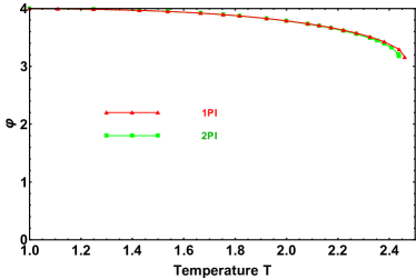
Figure 1: $\varphi$ - $T$ for 1PI and 2PI approaches, $T_{c,\text{1PI}}=2.4606$ and terminated $\varphi=3.15737$, $T_{c,\text{2PI}}=2.4390$ and $\varphi=3.17532$

Table 1: $T_{c}$ from various approximations and exact [20, 21, 5, 9] values.

Exact	BPW	SMF	SCCF	1PI	2PI
2.26918$\cdots$	2.885	2.142	2.595	2.4606	2.4390

In Table 1 we display $T_{c}$ from 1PI, 2PI, as well as the SCCF and SMF results [5, 9], together with either exact or approximate values from series estimates [20]. For the 2D square lattice Ising model, 1PI gives $T_{c}=2.4606$, and 2PI gives $T_{c}=2.4390$, both closer to the exact result than the BPW approximation and self-consistent correlated field method(SCCF).

According to fluctuation-dissipation theorem, we can get the susceptibility $\chi_{ij}$ with following relation:

$$\chi_{ij}=\frac{\delta\langle\sigma_{i}\rangle}{\delta h_{j}}=\beta\langle\sigma_{i}\sigma_{j}\rangle-\beta\langle\sigma_{i}\rangle\langle\sigma_{j}\rangle$$ (42)

The Fourier transform of the susceptibility $\chi_{ij}$ is

$$\chi_{ij}=\sum_{\alpha=x,y}\int^{\pi}_{-\pi}\frac{d^{2}k}{(2\pi)^{2}}\exp(-ik_{\alpha}(i_{\alpha}-j_{\alpha}))\chi(k)$$ (43)

The zero momentum susceptibility, which we denote as $\chi$, can be obtained from Eq(20, 41) with the following expression:

$$\chi= \beta\sum_{m}\left(\langle\sigma_{m}\sigma_{0}\rangle-\langle\sigma_{0}\rangle^{2}\right)=\beta\sum_{m}\left(J^{-1}_{m,i}J^{-1}_{0,j}G_{ij}-\beta^{-1}J^{-1}_{m,0}\right)$$ (44)

$$= \beta\left(J^{-2}(0)G(0)-\beta^{-1}J^{-1}(0)\right)$$

Here $G(0)$ refers to $G_{\text{full}}(0)$ or $G_{\text{ext}}(0)$, under 1PI or 2PI approximation, respectively. The numerical results are plotted in Fig.2, both susceptibility will diverge at its corresponding $T_{c}$.

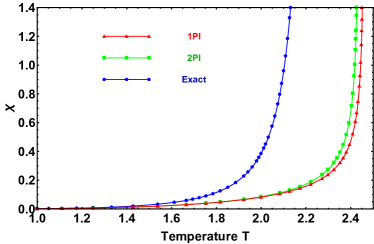
Figure 2: $\chi$ - $T$ from 1PI, 2PI approaches and exact value from low temperature expansion series[22, 23].

We also compare results for finite size lattices (subject to periodic boundary conditions) with Monte Carlo results. And the results are illustrated in Fig.3, under two different temperatures. For the finite size lattice of $N\times N$ with periodic boundary conditions, the formula in the integration shall be substituted as

$$\frac{1}{\left(2\pi\right)^{2}}\int_{-\pi}^{\pi}dk_{x}\int_{-\pi}^{\pi}dk_{y}f\left(k_{x},k_{y}\right)\rightarrow\frac{1}{N^{2}}\sum\limits_{k_{x},k_{y}}f\left(k_{x},k_{y}\right)$$ (45)

where $f\left(k_{x},k_{y}\right)$ is a periodic function of $k_{x}$ and $k_{y}$ (periodicity is $2\pi$), and inside the summation, $k_{x}=\frac{2\pi}{N}i,i=0,N-1,k_{y}=\frac{2\pi}{N}j,j=0,N-1$ due to periodic boundary conditions.

It can be seen that our results show a significant improvement compared to the Mean-field approach, especially for a temperature closer to $T_{c}$. We also include the correlation function obtained by BPW method (or Bethe approximation) in Fig. 3 for comparison. The BPW calculation of the correlation is highly non trivial and complex. It was only studied quite recently, see [24] and references therein. BPW method was particular useful for studying Ising model (also useful for Random Ising model), however the generalizations to other models are too complex. BPW result is better than the field theoretical result for the correlation function below the real critical temperature ($T_{c}=2.26918$), however the critical temperature obtained by BPW method is $T_{c}=2.885$, worse than the critical temperature obtained by the field theoretical method (for 1PI,$T_{c}=2.4606$, and for 2PI, $T_{c}=2.4390$ ).

Although the deviation of our approach for the correlation function with respect to MC is slightly larger than BPW method below the critical temperature, however, the field theoretical approach can easily generalize to quantum many body theory, and can be also applied to complicated spin models with continue symmetry , for example XY model and Heisenberg model, etc.

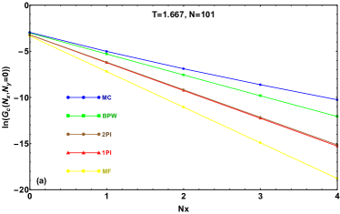
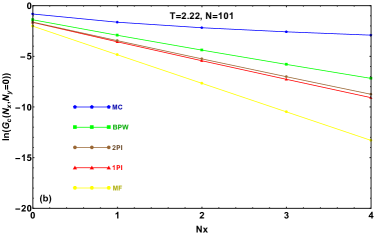
Figure 3: The logarithm of Green’s function at (a)$T=1.667$, (b)$T=2.22$ for $101\times 101$ for square lattice along the x direction. The regular pentagons are results by Monte Carlo simulation, green squares are BPW results ([24] and references therein), red triangles and brown septangles are 1PI and 2PI results respectively. The results from mean-field approach are denoted by yellow hexagons.

V conclusion

In conclusion, we calculate the critical temperature, susceptibility and Green function nonperturbatively with two kind field theories developed by the Dyson-Schwinger theory and the $\Phi$-derivable theory at leading order fluctuation correction. With relative low cost, both method are able to give fairly good predictions of $T_{c}$ for the Ising model. In the area far away from critical point, the susceptibility and Green function obtained from our method is quite accurate comparing with exact solution. This is a systemic approach which can be used to treat more complex spin models. The methods will preserve fundamental identities, like the fluctuation dissipation relation and WTI identities for systems with continue symmetries, which are very crucial for giving consistent descriptions of such systems.

References

• Ising [1925] E. Ising, Beitrag zur theorie des ferromagnetismus, Zeitschrift für Physik 31, 253 (1925).
• Onsager [1944] L. Onsager, Crystal statistics. i. a two-dimensional model with an order-disorder transition, Physical Review 65, 117 (1944).
• Kuzemsky [2009] A. Kuzemsky, Statistical mechanics and the physics of many-particle model systems, Physics of Particles and Nuclei 40, 949 (2009).
• Weiss et al. [1907] P. Weiss, P. Weiss, and E. Stoner, Magnetism ond atomic structure, J. phys 6, 667 (1907).
• Wysin and Kaplan [2000] G. Wysin and J. Kaplan, Correlated molecular-field theory for ising models, Physical Review E 61, 6399 (2000).
• Bethe [1935] H. A. Bethe, Statistical theory of superlattices, Proceedings of the Royal Society of London. Series A-Mathematical and Physical Sciences 150, 552 (1935).
• Peierls [1936] R. Peierls, On ising’s model of ferromagnetism, in Mathematical Proceedings of the Cambridge Philosophical Society, Vol. 32 (Cambridge University Press, 1936) pp. 477–481.
• Weiss [1948] P. R. Weiss, The application of the bethe-peierls method to ferromagnetism, Physical Review 74, 1493 (1948).
• Zhuravlev [2005] K. K. Zhuravlev, Molecular-field theory method for evaluating critical points of the ising model, Physical Review E 72, 056104 (2005).
• Yamamoto [2009] D. Yamamoto, Correlated cluster mean-field theory for spin systems, Physical Review B 79, 144427 (2009).
• Viana et al. [2014] J. R. Viana, O. R. Salmon, J. R. de Sousa, M. A. Neto, and I. T. Padilha, An effective correlated mean-field theory applied in the spin-1/2 ising ferromagnetic model, Journal of magnetism and magnetic materials 369, 101 (2014).
• Luttinger and Ward [1960] J. M. Luttinger and J. C. Ward, Ground-state energy of a many-fermion system. ii, Physical Review 118, 1417 (1960).
• Baym and Kadanoff [1961] G. Baym and L. P. Kadanoff, Conservation laws and correlation functions, Physical Review 124, 287 (1961).
• Cornwall et al. [1974] J. M. Cornwall, R. Jackiw, and E. Tomboulis, Effective action for composite operators, Physical Review D 10, 2428 (1974).
• Kovner and Rosenstein [1989] A. Kovner and B. Rosenstein, Covariant gaussian approximation. i. formalism, Physical Review D 39, 2332 (1989).
• Van Hees and Knoll [2002] H. Van Hees and J. Knoll, Renormalization in self-consistent approximation schemes at finite temperature. iii. global symmetries, Physical Review D 66, 025028 (2002).
• Amit and Martin-Mayor [2005] D. J. Amit and V. Martin-Mayor, Field theory, the renormalization group, and critical phenomena: graphs to computers (World Scientific Publishing Company, 2005).
• Wang et al. [2017] J. Wang, D. Li, H. Kao, and B. Rosenstein, Covariant gaussian approximation in ginzburg–landau model, Annals of Physics 380, 228 (2017).
• Rosenstein and Kovner [1989] B. Rosenstein and A. Kovner, Covariant gaussian approximation. ii. scalar theories, Physical Review D 40, 504 (1989).
• Fisher [1967] M. E. Fisher, The theory of equilibrium critical phenomena, Reports on progress in physics 30, 615 (1967).
• Ashcroft et al. [1976] N. W. Ashcroft, N. D. Mermin, et al.Solid state physics, Vol. 2005 (holt, rinehart and winston, new york London, 1976).
• Au-Yang and Perk [2002] H. Au-Yang and J. H. Perk, Correlation functions and susceptibility in the z-invariant ising model, in MathPhys Odyssey 2001 (Springer, 2002) pp. 23–48.
• Orrick et al. [2001] W. Orrick, B. Nickel, A. Guttmann, and J. Perk, The susceptibility of the square lattice ising model: new developments, Journal of Statistical Physics 102, 795 (2001), for the complete set of series coefficients see https://blogs.unimelb.edu.au/tony-guttmann/.
• Ricci-Tersenghi [2012] F. Ricci-Tersenghi, The bethe approximation for solving the inverse ising problem: a comparison with other inference methods, Journal of Statistical Mechanics: Theory and Experiment 2012, P08015 (2012).