Pseudorandom sequences derived from automatic sequences

Abstract

Many automatic sequences, such as the Thue-Morse sequence or the Rudin-Shapiro sequence, have some desirable features of pseudorandomness such as a large linear complexity and a small well-distribution measure. However, they also have some disastrous properties in view of certain applications. For example, the majority of possible binary patterns never appears in automatic sequences and their correlation measure of order $2$ is extremely large.

Certain subsequences, such as automatic sequences along squares, may keep the good properties of the original sequence but avoid the bad ones.

In this survey we investigate properties of pseudorandomness and non-randomness of automatic sequences and their subsequences and present results on their behaviour under several measures of pseudorandomness including linear complexity, correlation measure of order $k$, expansion complexity and normality. We also mention some analogs for finite fields.

Keywords — automatic sequences, pseudorandomness, linear complexity, maximum order complexity, well-distribution measure, correlation measure, expansion complexity, normality, finite fields

2020 Mathematics Subject Classification — 11A63, 11B85, 11K16, 11K31, 11K36, 11K45, 11T71, 68R15, 94A55, 94A60

1 Introduction

Pseudorandom sequences are sequences generated by deterministic algorithms which shall simulate randomness. In contrast to truly random sequences they are not random at all but guarantee certain desirable features and are reproducible.

Automatic sequences, see Section 2 below for the definition, have some of these desirable features but also some undesirable ones.

For example, the Thue-Morse sequence $(t_{n})$, defined by (2.2) below,

• has large $N$th linear complexity, see Section 3,

• has large $N$th maximum-order complexity, see Section 4,

• is balanced and has a small well-distribution measure, see Section 5.

However, the Thue-Morse sequence

• has a very large correlation measure of order $2$, see Section 5,

• a very small expansion complexity, see Section 6,

• and there are short patterns such as $000$ and $111$ which do not appear in the sequence and its subword complexity is only linear, see Section 7.

Hence, despite some nice features this sequence is not looking random at all, see Figure 1. The same is true for the Rudin-Shapiro sequence $(r_{n})$ defined by (2.3) below and many other related sequences.

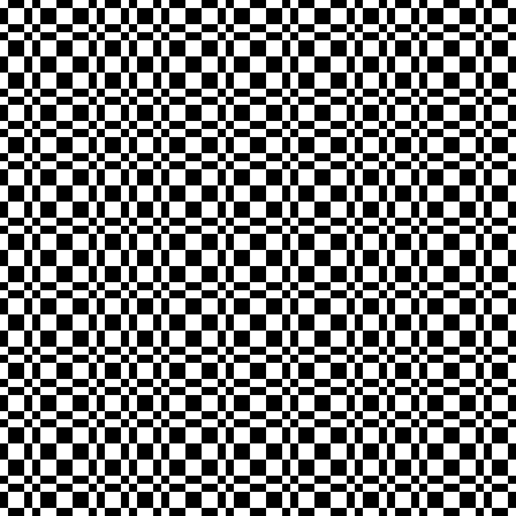
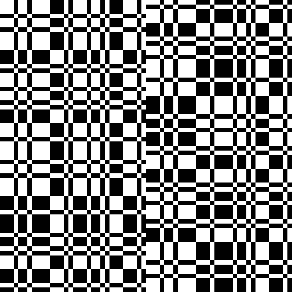
Figure 1: The first $4096$ elements of the Thue-Morse (left) and Rudin-Shapiro (right) sequence split into $64$ rows of each $64$ sequence elements. Zeros are represented by white, ones are represented by black.

Taking suitable subsequences may destroy the non-random structure of the original sequence but may keep the desirable features of pseudorandomness. Promising candidates for such subsequences are

• along squares, cubes, bi-squares, … or any polynomial values for any polynomial $f$ of degree at least $2$ with $f(\mathbb{N}_{0})\subset\mathbb{N}_{0}$,

• along primes,

• along the Piateski-Shapiro sequence $\lfloor n^{c}\rfloor$, $1<c<2$,

• and along geometric sequences such as $3^{n}$.

For example, the Thue-Morse sequence and the Rudin-Shapiro sequence along squares still

• have a large maximum-order complexity and thus a large linear complexity, see Section 4,

• and are asymptotically balanced, see Section 7.

Moreover, in contrast to the original sequence they

• have unbounded expansion complexity, see Section 6,

• and are normal, that is, asymptotically each pattern appears with the right frequency in the sequence, see Section 7.

Roughly speaking, they look much more random than the original sequences, see Figure 2.

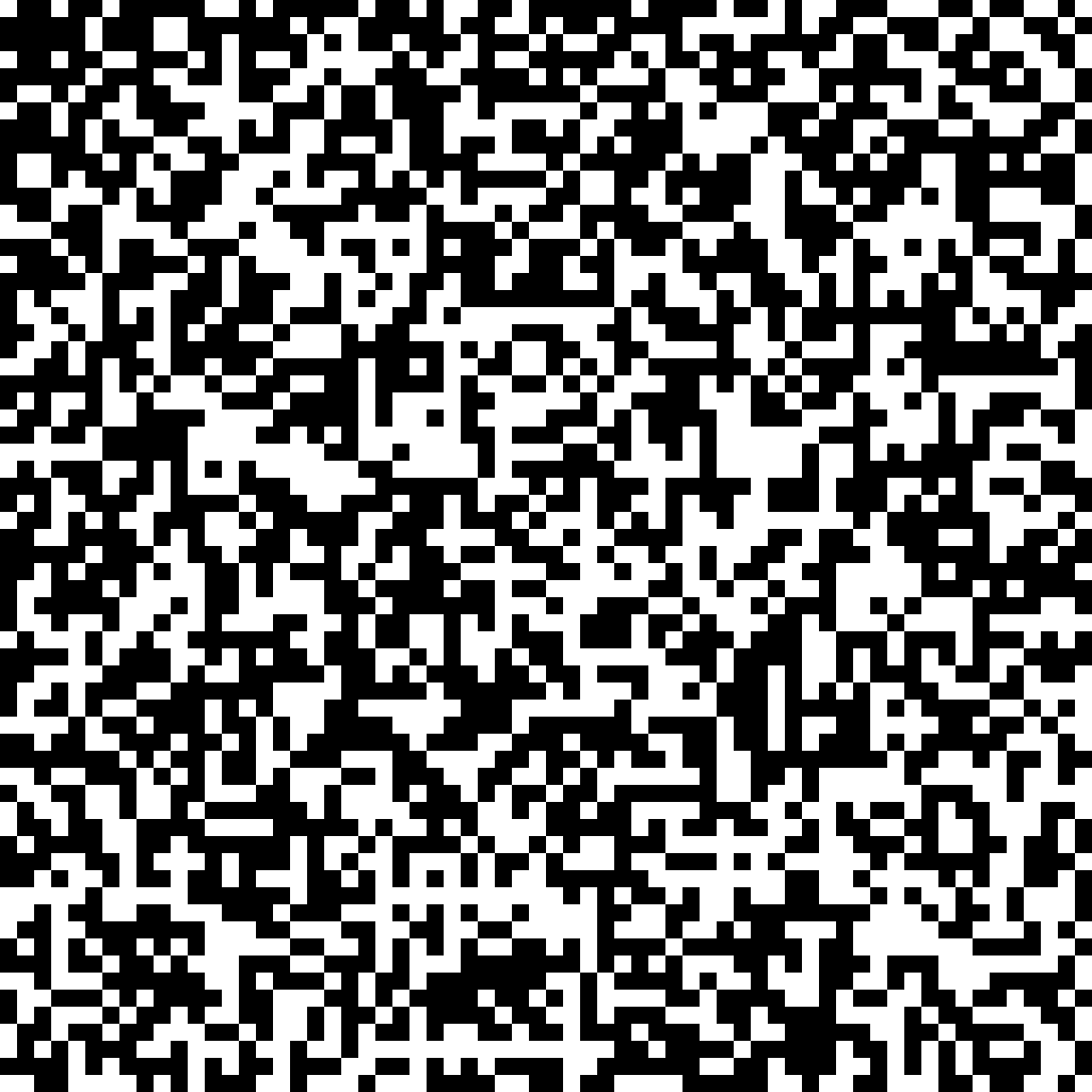
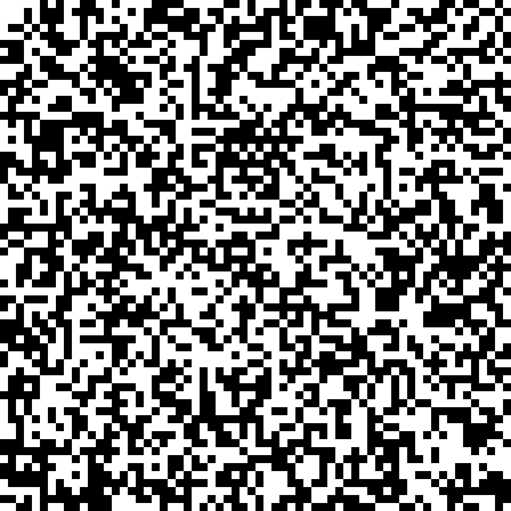
Figure 2: The first $4096$ elements of the Thue-Morse (left) and Rudin-Shapiro (right) sequence along squares split into $64$ rows of each $64$ sequence elements. Zeros are represented by white, ones are represented by black.

Still some questions about these sequences remain open such as upper bounds on the correlation measure of order $k$ and on the expansion complexity. We will state explicitly some selected open problems to motivate future research.

We also look for further directions in Section 8. In particular, we discuss analogs of the Thue-Morse and Rudin-Shapiro sequence and their subsequences in the setting of finite fields.

For general background on automatic sequences and finite automata we refer to the monograph of Allouche and Shallit [7] and also to [6, 8, 34, 35]. For surveys on pseudorandom sequences see [43, 66, 76, 85, 97].

2 Finite automata and automatic sequences

Roughly speaking, a sequence is automatic if it is generated by a finite automaton, see Definition 2.2 below.

Definition 2.1.

Let $k\geq 2$ be an integer. A finite $k$-automaton ${\mathcal{A}}$ is a $6$-tuple

$${\mathcal{A}}=(Q,\Sigma,\delta,q_{0},\varphi,\Delta),$$

where

• $Q$ is a finite set of states,

• $\Sigma=\{0,1,\ldots,k-1\}$ is the input alphabet,

• $\delta:Q\times\Sigma\rightarrow Q$ is the transition function,

• $q_{0}\in Q$ is the initial state,

• $\Delta$ is the output alphabet

• and $\varphi:Q\rightarrow\Delta$ is the output function.

For example, the Thue-Morse automaton, see Figure 3, is a $2$-automaton with $2$ states and the Rudin-Shapiro automaton, see Figure 4, is a $2$-automaton with $4$ states, both with inputs and outputs in $\Sigma=\Delta=\{0,1\}$.

Figure 3: Thue-Morse automaton

Figure 4: Rudin-Shapiro automaton

Definition 2.2.

Let $\Delta$ be a finite set. A sequence $(s_{n})$ over $\Delta$ is called a $k$-automatic sequence if there is a $k$-automaton ${\mathcal{A}}$ such that on input of the digits $n_{0},n_{1},\ldots$ of the $k$-ary expansion of $n\geq 0$,

$$n=\sum_{i\geq 0}n_{i}k^{i},\quad n_{i}\in\{0,1,\dots,k-1\},$$ (2.1)

${\mathcal{A}}$ outputs the sequence element $s_{n}\in\Delta$. Reading of the digits of $n$ starting with the most significant digit is called direct whereas reading starting with the least significant digit $n_{0}$ is called reverse. If not stated otherwise, we use reverse reading. Finally, a sequence is called automatic if it is $k$-automatic for some $k$.

Example (Thue-Morse sequence).

The Thue-Morse sequence $(t_{n})$ is a $2$-automatic sequence generated by the Thue-Morse automaton, Figure 3. This sequence is the sequence of the sum of digits modulo $2$. The sequence begins with

$$011010011001\dots,$$

see also Figure 1 for a picture of the first $4096$ sequence elements. It follows from the defining automaton, see Figure 3, that $(t_{n})$ satisfies the following recurrence relation

$$t_{n}=\left\{\begin{array}[]{cl}t_{n/2}&\mbox{if $n$ is even},\\ t_{(n-1)/2}+1\bmod 2&\mbox{if $n$ is odd},\end{array}\right.\quad n=1,2,\ldots$$ (2.2)

with initial value $t_{0}=0$.

Example (Rudin-Shapiro sequence).

The Rudin-Shapiro sequence $(r_{n})$ is a $2$-automatic sequence generated by the Rudin-Shapiro automaton, see Figure 4. The sequence begins with

$$000100100001\dots,$$

see also Figure 1 for a picture of the first $4096$ sequence elements. It follows from the defining automaton, see Figure 4, that $(r_{n})$ satisfies the following recurrence relation

$$r_{n}=\left\{\begin{array}[]{cl}r_{\lfloor n/2\rfloor}+1\bmod 2&\mbox{if $n\equiv 3\bmod 4$},\\ r_{\lfloor n/2\rfloor}&\mbox{otherwise},\end{array}\right.\quad n=1,2,\ldots$$ (2.3)

with initial value $r_{0}=0$.

The sequence $((-1)^{r_{n}})$ over $\{-1,+1\}$ is also called Rudin-Shapiro sequence in the literature. Here we study only the sequence $(r_{n})$ over $\{0,1\}$.

Example (Pattern sequences).

For a pattern $P\in\Delta^{\ell}\setminus\{(0,\dots,0)\}$ of length $\ell$ over $\Delta=\{0,1,\dots,k-1\}$ define the sequence $(p_{n})$ by

$$p_{n}=e_{P}(n)\bmod k,\quad 0\leq p_{n}<k,\quad n=0,1,\dots,$$

where $e_{P}(n)$ is the number of occurrences of $P$ in the $k$-ary expansion of $n$. The sequence $(p_{n})$ over $\Delta$ satisfies the following recurrence relation

$$p_{n}=\left\{\begin{array}[]{cl}p_{\lfloor n/k\rfloor}+1\bmod k&\text{if }n\equiv a\bmod k^{\ell},\\ p_{\lfloor n/k\rfloor}&\text{otherwise,}\end{array}\right.n=1,2,\dots$$ (2.4)

with initial value $p_{0}=0$, where $a=a(P)$ is the integer $0<a<k^{\ell}$ such that its $k$-ary expansion corresponds to the pattern $P$.

Classical examples for binary pattern sequences are the Thue-Morse sequence with

$$k=2,\quad\ell=1,\quad P=1\quad\mbox{and}\quad a=1,$$

and the Rudin-Shapiro sequence with

$$k=2,\quad\ell=2,\quad P=11\quad\mbox{and}\quad a=3.$$

In particular, if $n_{0},n_{1},\dots$ are the bits of the non-negative integer taken from (2.1) with $k=2$, then

$$t_{n}=\sum_{i=0}^{\infty}n_{i}\bmod 2\quad\mbox{and}\quad r_{n}=\sum_{i=0}^{\infty}n_{i}n_{i+1}\bmod 2.$$ (2.5)

Example (Rudin-Shapiro-like sequence).

Lafrance, Rampersad and Yee [51] introduced a Rudin-Shapiro-like sequence $(\ell_{n})$ which is based on the number of occurrences of the pattern $10$ as a scattered subsequence in the binary representation, (2.1) with $k=2$, of $n$. That is, $\ell_{n}$ is the parity of the number of pairs $(i,j)$ with $i>j$ and $(n_{i},n_{j})=(1,0)$. See Figure 5 for its defining automaton.

Figure 5: Rudin-Shapiro-like automaton with direct reading

This sequence can also be defined by

$$\ell_{2n+1}=\ell_{n}\quad\mbox{and}\quad\ell_{2n}=\ell_{n}+t_{n}\bmod 2,$$ (2.6)

see [51, $(1)$ and $(2)$], with initial value $\ell_{0}=0$ and where $(t_{n})$ is the Thue-Morse sequence.

Example (Baum-Sweet sequence).

The Baum-Sweet sequence $(b_{n})$ is a $2$-automatic sequence defined by the rule $b_{0}=1$ and for $n\geq 1$

$$b_{n}=\left\{\begin{array}[]{cl}1&\text{if the binary representation of $n$ contains no block of}\\ &\text{consecutive $0$'s of odd length,}\\ 0&\text{otherwise.}\end{array}\right.$$

Equivalently, we have for $n\geq 1$ of the form $n=4^{\ell}m$ with $4\nmid m$ that

$$b_{n}=\left\{\begin{array}[]{cl}0&\text{if $m$ is even},\\ b_{(m-1)/2}&\text{if $m$ is odd.}\end{array}\right.$$ (2.7)

The sequence $(b_{n})$ is generated by the Baum-Sweet automaton in Figure 6.

Figure 6: Baum-Sweet automaton

Example (Characteristic sequence of sums of three squares).

Consider the characteristic sequence $(c_{n})$ of the set of integers which are sums of three squares of an integer, that is,

$$c_{n}=\left\{\begin{array}[]{cl}1&\text{if }n=a^{2}+b^{2}+c^{2}\text{ for some non-negative integers $a,b,c$,}\\ 0&\text{otherwise.}\end{array}\right.$$

By Legendre’s three-square theorem, we have the equivalent definition

$$c_{n}=\left\{\begin{array}[]{cl}1&\text{if $n$ is not of the form $n=4^{\ell}(8k+7)$,}\\ 0&\text{otherwise.}\end{array}\right.$$ (2.8)

See Figure 7 for the defining automaton.

Figure 7: Automaton of the characteristic sequence of sums of three squares with reverse reading

Example (Regular paper-folding sequence).

The regular paper-folding sequence $(v_{n})$ with initial value $v_{0}\in\{0,1\}$ is defined as follows. If $n=2^{k}m$ with an odd $m$, then

$$v_{n}=\left\{\begin{array}[]{ll}1,&m\equiv 1\bmod 4,\\ 0,&m\equiv 3\bmod 4,\end{array}\right.\quad n=1,2,\ldots$$ (2.9)

Its defining automaton with four states is given in Figure 8.

Figure 8: Regular paper-folding automaton

Example (An automatic apwenian sequence).

Any binary sequence $(a_{n})$ satisfying $a_{0}=1$ and

$$a_{2n+2}=a_{2n+1}+a_{n}\bmod 2,\quad n=0,1,\ldots$$

is called apwenian, see for example [4]. Apwenian sequences which are $2$-automatic are characterized in [4]. For example, the sequence $(w_{n})$ defined by

$$w_{2n}=1\quad\mbox{and}\quad w_{2n+1}=w_{n}+1\bmod 2,\quad n=0,1,\ldots$$ (2.10)

is apwenian and defined by the automaton in Figure 9.

Figure 9: Apwenian automaton

In addition to the examples above, all ultimately periodic sequences are $k$-automatic for all integers $k\geq 2$, see [7, Theorem 5.4.2]. Moreover, by Cobham’s theorem [7, Theorem 11.2.1], if a sequence $(s_{n})$ is both $k$-automatic and $\ell$-automatic and $k$ and $\ell$ are multiplicatively independent, then $(s_{n})$ is ultimately periodic.

For a prime power $k=q$, $k$-automatic sequences $(s_{n})$ over the finite field $\Delta=\mathbb{F}_{q}$ can be characterized by a result of Christol, see [17] for prime $q$ and [18] for prime power $q$ as well as [7, Theorem 12.2.5].

Theorem 2.1.

Let

$$G(x)=\sum_{n=0}^{\infty}s_{n}x^{n}\in\mathbb{F}_{q}\llbracket x\rrbracket$$

be the generating function of the sequence $(s_{n})$ over $\mathbb{F}_{q}$. Then $(s_{n})$ is $q$-automatic if and only if $G(x)$ is algebraic over $\mathbb{F}_{q}(x)$, that is, there is a polynomial $h(x,y)\in\mathbb{F}_{q}[x,y]\setminus\{0\}$ such that $h(x,G(x))=0$.

Note that for all $m=1,2,\ldots$ a sequence is $k$-automatic if and only if it is $k^{m}$-automatic by [7, Theorem 6.6.4] and even a slightly more general version of Christol’s result holds: For a prime $p$ and positive integers $m$ and $r$, $(s_{n})$ is $p^{m}$-automatic over $\mathbb{F}_{p^{r}}$ if and only if $G(x)$ is algebraic over $\mathbb{F}_{p^{r}}(x)$.

Example.

The generating function $G(x)$ of the Thue-Morse sequence $(t_{n})$ over $\mathbb{F}_{2}$ satisfies $h(x,G(x))=0$ with

$$h(x,y)=(x+1)^{3}y^{2}+(x+1)^{2}y+x.$$ (2.11)

The generating function $G(x)$ of the Rudin-Shapiro sequence $(r_{n})$ over $\mathbb{F}_{2}$ satisfies $h(x,G(x))=0$ with

$$h(x,y)=(x+1)^{5}y^{2}+(x+1)^{4}y+x^{3}.$$ (2.12)

In general, for prime $p$ the generating function $G(x)$ of the $p$-ary pattern sequence $(p_{n})$ over $\mathbb{F}_{p}$ with respect to the pattern $P$ of length $\ell$ satisfies $h(x,G(x))=0$ with

$$h(x,y)=(x-1)^{p^{\ell}+p-1}y^{p}-(x-1)^{p^{\ell}}y-x^{a(P)}.$$ (2.13)

The generating function $G(x)$ of the Rudin-Shapiro-like sequence $(\ell_{n})$ over $\mathbb{F}_{2}$ defined by (2.6) satisfies $h(x,G(x))=0$ with

$$h(x,y)=(x+1)^{8}y^{4}+(x^{6}+x^{5}+x^{2}+x)y^{2}+(x+1)^{4}y+x^{2},$$ (2.14)

see [93, Proof of Theorem 2].

The generating function $G(x)$ of the Baum-Sweet sequence $(b_{n})$ over $\mathbb{F}_{2}$ satisfies $h(x,G(x))=0$ with

$$h(x,y)=y^{3}+xy+1.$$ (2.15)

The generating function $G(x)$ of the characteristic sequence $(c_{n})$ of sums of three squares (2.8) over $\mathbb{F}_{2}$ satisfies $h(x,G(x))=0$ with

$$h(x,y)=(x+1)^{8}(y+y^{4})+x^{6}+x^{5}+x^{3}+x^{2}+x,$$ (2.16)

see [45, Equation (7)].

The generating function $G(x)$ of the regular paper-folding sequence $(v_{n})$ over $\mathbb{F}_{2}$ satisfies $h(x,G(x))=0$ with

$$h(x,y)=(x+1)^{4}(y^{2}+y)+x.$$ (2.17)

The generating function $G(x)$ of the apwenian sequence $(w_{n})$ over $\mathbb{F}_{2}$ defined by (2.10) satisfies

$$h(x,y)=(x+1)(xy^{2}+y)+1.$$ (2.18)

3 Linear complexity

The linear complexity is a figure of merit of pseudorandom sequences introduced to capture undesirable linear structure in a sequence. It originates in cryptography and provides a test of randomness which is a standard tool to filter sequences with non-randomness properties and is implemented in many test suites such as NIST and TestU01 [82, 53].

Definition 3.1.

The $N$th linear complexity $L(s_{n},N)$ of a sequence $(s_{n})$ over $\mathbb{F}_{q}$ is the length $L$ of a shortest linear recurrence relation satisfied by the first $N$ elements of $(s_{n})$,

$$s_{n+L}=c_{L-1}s_{n+L-1}+\dots+c_{1}s_{n+1}+c_{0}s_{n},\quad 0\leq n\leq N-L-1,$$

for some $c_{0},\ldots,c_{L-1}\in\mathbb{F}_{q}$. We use the convention that $L(s_{n},N)=0$ if the first $N$ elements of $(s_{n})$ are all zero and $L(s_{n},N)=N$ if $s_{0}=\dots=s_{N-2}=0\neq s_{N-1}$. The sequence $(L(s_{n},N))_{N=1}^{\infty}$ is called linear complexity profile of $(s_{n})$ and

$$L(s_{n})=\sup_{N\geq 1}L(s_{n},N)$$

is the linear complexity of $(s_{n})$.

Clearly, $0\leq L(s_{n},N)\leq N$ and $L(s_{n},N)\leq L(s_{n},N+1)$.

For truly random sequences $(s_{n})$ the expected value of its $N$th linear complexity $L$ is

$$\frac{N}{2}+O(1),$$

see for example [70, Theorem 10.4.42]. Deviations of order of magnitude $\log N$ must appear for infinitely many $N$. More precisely, for a prime power $q$ consider the following probability measure of sequences over $\mathbb{F}_{q}$ determined by

$$\mathbb{P}\left[(s_{n})\in\mathbb{F}_{q}^{\infty}:(s_{0},\dots,s_{\ell-1})=(c_{0},\dots,c_{\ell-1})\right]=q^{-\ell},\quad c_{0},\dots,c_{\ell-1}\in\mathbb{F}_{q}.$$ (3.1)

Then we have the following result on the deviation from the expected value, see[74, Theorem 10].

Theorem 3.1.

We have

$$\limsup_{N\rightarrow\infty}\frac{L(s_{n},N)-N/2}{\log N}=\frac{1}{2\log q},$$

and

$$\liminf_{N\rightarrow\infty}\frac{L(s_{n},N)-N/2}{\log N}=\frac{-1}{2\log q}$$

with probability one with respect to the probability measure (3.1).

It is well-known [73, Lemma 1] that $L(s_{n})<\infty$ if and only if $(s_{n})$ is ultimately periodic, that is, its generating function is rational: $G(x)=g(x)/f(x)$ with polynomials $g(x),f(x)\in\mathbb{F}_{q}[x]$.

The $N$th linear complexity is a measure for the unpredictability of a sequence. A large $N$th linear complexity, up to sufficiently large $N$, is necessary, but not sufficient, for cryptographic applications. Sequences of small linear complexity are also weak in view of Monte-Carlo methods, see [27, 28, 29, 30]. For more background on linear complexity and related measures of pseudorandomness we refer to [70, Section 10.4] and [75, 97, 99].

Mérai and Winterhof [68] showed that automatic sequences which are not ultimately periodic possess large $N$th linear complexity.

Theorem 3.2.

Let $q$ be a prime power and $(s_{n})$ be a $q$-automatic sequence over $\mathbb{F}_{q}$ which is not ultimately periodic. Let $h(x,y)=h_{0}(x)+h_{1}(x)y+\dots+h_{d}(x)y^{d}\in\mathbb{F}_{q}[x,y]$ be a non-zero polynomial with $h(G(x),x)=0$ with no rational zero. Put

$$M=\max_{0\leq i\leq d}\{\deg h_{i}-i\}.$$

Then we have

$$\frac{\displaystyle N-M}{d}\leq L(s_{n},N)\leq\frac{\displaystyle(d-1)N+M+1}{d}.$$

See also [100] for the special case $d=2$.

The idea of the proof of Theorem 3.2 is that small $N$th linear complexity profile gives a good rational approximation to the generating function. However, transcendental elements over $\mathbb{F}_{q}(x)$ are not well-approximated.

Namely, since $(s_{n})$ is not ultimately periodic, $G(x)=\sum_{n=0}^{\infty}s_{n}x^{n}\not\in\mathbb{F}_{q}(x)$ is not rational by [73, Lemma 1].

Let $g(x)/f(x)\in\mathbb{F}_{q}(x)$ be a rational zero of $h(x,y)$ modulo $x^{N}$ with $\deg(f)\leq L(s_{n},N)$ and $\deg(g)<L(s_{n},N)$. More precisely, put $L=L(s_{n},N)$. Then we have

$$\sum_{\ell=0}^{L}c_{\ell}s_{n+\ell}=0\quad\mbox{for }0\leq n\leq N-L-1$$

for some $c_{0},\ldots,c_{L}\in\mathbb{F}_{p}$ with $c_{L}=-1$. Take

$$f(x)=\sum_{\ell=0}^{L}c_{\ell}x^{L-\ell}$$

and

$$g(x)=\sum_{m=0}^{L-1}\left(\sum_{\ell=L-m}^{L}c_{\ell}s_{m+\ell-L}\right)x^{m}$$

and verify

$$f(x)G(x)\equiv g(x)\bmod x^{N}.$$

Then

$$h_{0}(x)f^{d}(x)+h_{1}(x)g(x)f^{d-1}(x)+\dots+h_{d}(x)g(x)^{d}=K(x)x^{N}.$$

Here $K(x)\neq 0$ since $h(x,y)$ has no rational zero. Comparing the degrees of both sides we get

$$dL+M\geq N$$

which gives the lower bound.

The upper bound for $N=1$ is trivial. For $N\geq 2$ the result follows from the well-known bound, see for example [30, Lemma 3],

$$L(s_{n},N)\leq\max\left\{L(s_{n},N-1),N-L(s_{n},N-1)\right\}$$

by induction.

The bound in Theorem 3.2 combined with (2.11)-(2.18) gives the following estimates for the $N$th linear complexity of the Thue-Morse sequence $(t_{n})$ defined by (2.2)

$$\left\lceil\frac{N-1}{2}\right\rceil\leq L(t_{n},N)\leq\left\lfloor\frac{N}{2}\right\rfloor+1,$$ (3.2)

of the Rudin-Shapiro sequence $(r_{n})$ defined by (2.3) and the regular paper-folding sequence $(v_{n})$ defined by (2.9)

$$\left\lceil\frac{N-3}{2}\right\rceil\leq L(r_{n},N),L(v_{n},N)\leq\left\lfloor\frac{N}{2}\right\rfloor+2,$$ (3.3)

of the $p$-ary pattern sequence $(p_{n})$ defined by (2.4) with any pattern $P$ of length $\ell$

$$\left\lceil\frac{N+1}{p}\right\rceil-p^{\ell-1}\leq L(p_{n},N)\leq\left\lfloor\frac{(p-1)N}{p}\right\rfloor+p^{\ell-1},$$

of the Rudin-Shapiro-like sequence $(\ell_{n})$ defined by (2.6)

$$\left\lceil\frac{N}{4}\right\rceil-1\leq L(\ell_{n},N)\leq\left\lfloor\frac{3N+5}{4}\right\rfloor,$$

of the Baum-Sweet sequence $(b_{n})$ defined by (2.7)

$$\left\lceil\frac{N}{3}\right\rceil\leq L(b_{n},N)\leq\left\lfloor\frac{2N+1}{3}\right\rfloor,$$

of the characteristic sequence $(c_{n})$ of sums of three squares defined by (2.8)

$$\left\lceil\frac{N-7}{4}\right\rceil\leq L(c_{n},N)\leq\left\lfloor\frac{3N}{4}\right\rfloor+2$$

and of the apwenian sequence $(w_{n})$ defined by (2.10)

$$L(w_{n},N)=\left\lfloor\frac{N+1}{2}\right\rfloor.$$ (3.4)

Note that the bound (3.2) is also true for the dual $(t^{\prime}_{n})$ of the Thue-Morse sequence, that is, $t^{\prime}_{n}=1-t_{n}$, and apwenian sequences are characterized by the property (3.4), see [4]. Note that not all apwenian sequences are automatic.

The bounds (3.2) for the Thue-Morse sequence and (3.3) for the Rudin-Shapiro sequence are optimal. Using the continued fraction expansions of their generating functions, Mérai and Winterhof [68] determined the exact value of the $N$th linear complexity profiles of the Thue-Morse and Rudin Shapiro sequence.

Theorem 3.3.

The $N$th linear complexity of the Thue-Morse sequence is

$$L(t_{n},N)=2\left\lfloor\frac{N+2}{4}\right\rfloor,\quad N=1,2,\dots$$

and the $N$th linear complexity of the Rudin-Shapiro sequence is

$$L(r_{n},N)=\left\{\begin{array}[]{cc}6\left\lfloor N/12\right\rfloor+4,&N\equiv 4,5,6,7,8,9\bmod 12,\\ 6\left\lfloor(N+2)/12\right\rfloor,&\mbox{otherwise}.\end{array}\right.$$

The result can be extended to binary pattern sequences $(p_{n})$ defined by (2.4) with the all one pattern of length $\ell\geq 3$, that is, $a=2^{\ell}-1$.

It follows from Theorem 3.2, that if an automatic sequence is not ultimately periodic and its generating function has a quadratic minimal polynomial, that is $d=2$ in Theorem 3.2, then the deviation of the $N$th linear complexity from its expected value $N/2$ is bounded by $(M+1)/2$,

$$\left|L(s_{n},N)-\frac{N}{2}\right|\leq\frac{M+1}{2}.$$

Such sequences are said to have almost perfect or $(M+1)$-perfect linear complexity profile, see [73, 4].

Apwenian sequences are those sequences having $1$-perfect or just perfect linear complexity profile. The bounds (3.2) and (3.3) imply that the Thue-Morse sequence has $2$-perfect linear complexity profile and the Rudin-Shapiro sequence and the paper-folding sequence both have $4$-perfect linear complexity profile.

Although automatic sequences have some good pseudorandom properties including a desirable linear complexity profile, these sequences have also some strong non-randomness properties, see Sections 5, 6 and 7 below. Such randomness flaws may be avoided considering subsequences of automatic sequences. For example, the Thue-Morse and Rudin-Shapiro sequences along squares are not automatic, see Section 7 below, and seem to have $N$th linear complexity $N/2+O(\log N)$, see Figure 10.

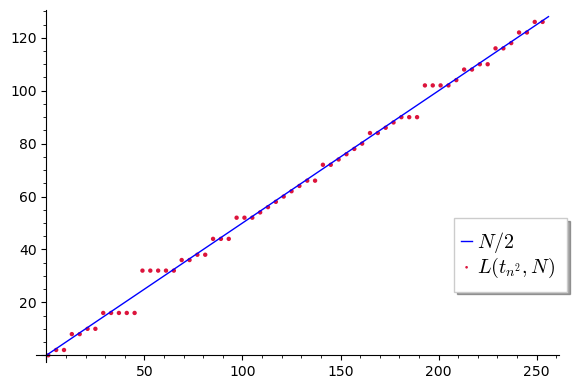
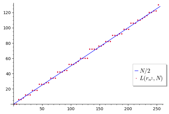
Figure 10: The $N$th linear complexity of the Thue-Morse (left) and Rudin-Shapiro (right) sequence along squares.

Problem 1.

Prove that the $N$th linear complexities of the Thue-Morse and Rudin-Shapiro sequences along squares satisfy

$$L(t_{n^{2}},N)=\frac{N}{2}+o(N)\quad\mbox{and}\quad L(r_{n^{2}},N)=\frac{N}{2}+o(N).$$

We remark, that lower bounds on the $N$th linear complexities of $(t_{n^{2}})$ and $(r_{n^{2}})$ of order of magnitude $\sqrt{N}$ follow from Theorem 4.2 and (4.1) in the next section.

Additional to these examples, the same problem is also open for other subsequences such as along other polynomial values, along primes etc.

4 Maximum order complexity

Maximum order (or nonlinear) complexity is a refinement of the linear complexity considering not only linear but any recurrence relation.

Definition 4.1.

The $N$th maximum order complexity $M(s_{n},N)$ is the smallest positive integer $M$ with

$$s_{n+M}=f(s_{n+M-1},\ldots,s_{n}),\quad 0\leq n\leq N-M-1,$$

for some mapping $f:\mathbb{F}_{2}^{M}\rightarrow\mathbb{F}_{2}$. The sequence $(M(s_{n},N))_{N=1}^{\infty}$ is called maximum order complexity profile.

Obviously, we have

$$M(s_{n},N)\leq L(s_{n},N)$$ (4.1)

and the maximum order complexity is a finer measure for the unpredictability of a sequence than the linear complexity. However, often the linear complexity is easier to analyze both theoretically and algorithmically.

Clearly, a sufficiently large maximum order complexity is needed for unpredictability and suitability in cryptography. However, sequences of very large maximum order complexity have also a very large autocorrelation or correlation measure of order $2$, see (5.6) below, and are not suitable for many applications including cryptography, radar, sonar and wireless communications.

The maximum order complexity was introduced by Jansen in [48, Chapter 3], see also [49]. The typical value for the $N$th maximum order complexity is of order of magnitude $\log N$, see [48, 49]. An algorithm for calculating the maximum order complexity profile of linear time and memory was presented by Jansen [48, 49] using the graph algorithm introduced by Blumer et al. [10].

The maximum order complexity of the Thue-Morse sequence was determined in [92, Theorem 1].

Theorem 4.1.

For $N\geq 4$, the $N$th maximum order complexity of the Thue-Morse sequence $(t_{n})$ satisfies

$$M(t_{n},N)=2^{\ell}+1,$$

where

$$\ell=\left\lceil\frac{\log(N/5)}{\log 2}\right\rceil.$$

It is easy to see that

$$\frac{N}{5}+1\leq M(t_{n},N)\leq 2\frac{N-1}{5}+1\quad\text{for}\;\;N\geq 4.$$ (4.2)

In Section 5 we will see that such a large maximum order complexity points to undesirable structure in a sequence.

The $N$th maximum order complexity of the Rudin-Shapiro sequence and some generalizations is also of order of magnitude $N$, see [92, Theorem 2]. In particular we have

$$M(r_{n},N)\geq\frac{N}{6}+1,\quad N\geq 4.$$ (4.3)

The maximum order complexity of the subsequences of the Thue-Morse and the Rudin-Shapiro sequence along squares are still large enough, see [91].

Theorem 4.2.

The $N$th maximum order complexities $M(t_{n^{2}},N)$ and $M(r_{n^{2}},N)$ of the subsequences $(t_{n^{2}})$ and $(r_{n^{2}})$ of the Thue-Morse and the Rudin-Shapiro sequence along squares satisfy

$$M(t_{n^{2}},N)\geq\sqrt{\frac{2N}{5}},\quad N\geq 21,\quad\mbox{and}$$

$$M(r_{n^{2}},N)\geq\sqrt{\frac{N}{8}},\quad N\geq 64.$$

We sketch the proof. First, let $t$ be the length of the longest subsequence of $(t_{n^{2}})$ that occurs at least twice with different successors among the first $N$ sequence elements. Then $M(t_{n^{2}},N)\geq t+1$. Hence the first inequality follows from

$$t_{(i+2^{\ell+1})^{2}}=t_{(i+2^{\ell+2})^{2}},\quad i=0,1,\ldots,\left\lfloor\sqrt{2^{\ell+2}-1}\right\rfloor$$

$$\mbox{and}\quad t_{(2^{\ell}+2^{\ell+1})^{2}}\neq t_{(2^{\ell}+2^{\ell+2})^{2}},$$

which can be shown by induction over $\ell\geq 2$, where $\ell$ is defined by $5\cdot 2^{\ell}<N\leq 5\cdot 2^{\ell+1}$.

The second bound follows from

$$r_{(i+2^{\ell+3})^{2}}=r_{(i+2^{\ell+4})^{2}},\quad i=0,1,\ldots,\left\lfloor\sqrt{2^{\ell+3}-1}\right\rfloor,$$

$$\mbox{and}\quad r_{(2^{\ell+2}+2^{\ell+3})^{2}}\neq r_{(2^{\ell+2}+2^{\ell+4})^{2}},$$

where $\ell$ is defined by $2^{\ell+5}\leq N<2^{\ell+6}$.

Figure 11 suggests that $\sqrt{N}$ is the right order of magnitude for the $N$th maximum order complexities of $(t_{n^{2}})$ and $(r_{n^{2}})$. For $N\geq 2^{2\ell+2}$ the same lower bound $\sqrt{N/8}$ is true for binary pattern sequences along squares with the all one pattern of length $\ell$, that is, $a=2^{\ell}-1$ for $\ell\geq 3$, see [91].

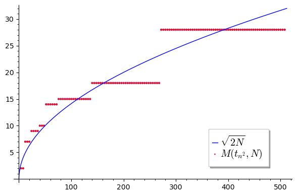
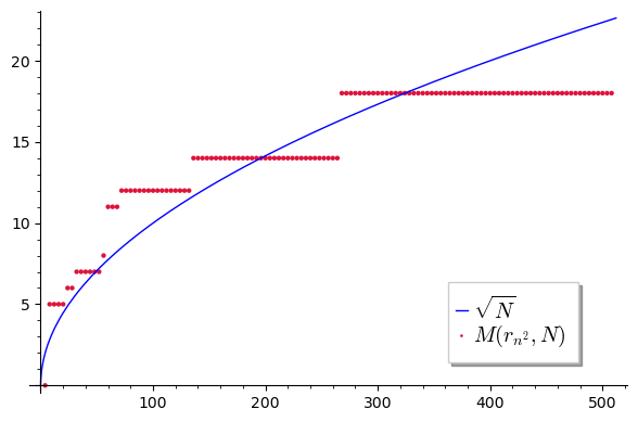
Figure 11: The $N$th maximum order complexity of the Thue-Morse (left) and Rudin-Shapiro (right) sequence along squares.

This result was extended by Popoli [79] to sequences along polynomial values of higher degrees $d$. However, the lower bounds are of order of magnitude $N^{1/d}$. Note that no better lower bounds are known for the $N$th linear complexity of these subsequences of automatic sequences.

The problem for other subsequences is still open as for example for subsequences along primes.

Problem 2.

Study the maximum-order complexity of the subsequences of the Thue-Morse and the Rudin-Shapiro sequence along primes.

The maximum order complexity of other automatic sequences has also been studied. Sun, Zeng and Lin [93] showed that the $N$th maximum order complexity of the Rudin-Shapiro-like sequence $(\ell_{n})$ defined by (2.6) is of order of magnitude $N$.

We remark, that in addition to automatic sequences based on the $k$-ary expansion (2.1) of integers, one can consider analogously sequences using other numeration systems.

In particular, consider the Fibonacci numbers defined by

$$F_{0}=0,~{}F_{1}=1\quad\mbox{and}\quad F_{n}=F_{n-1}+F_{n-2}\mbox{ for }n\geq 2.$$

Then the unique, see for example [7, Theorem 3.8.1], Zeckendorf expansion or Fibonacci expansion, of a positive integer $n$ is

$$n=\sum_{i=0}^{\infty}e_{i}F_{i+2},\quad\mbox{where }e_{i}\in\{0,1\}\mbox{ and }e_{i}e_{i+1}=0\mbox{ for }i=0,1,\ldots$$

Analogously to the Thue-Morse sum-of-digits sequence $(t_{n})$ and the Rudin-Shapiro sequence $(r_{n})$ which can be defined by (2.5) we can define and study the Zeckendorf sum-of-digits sequences modulo $2$ $(z_{n})$ and $(u_{n})$ defined by

$$z_{n}=\sum_{i=0}^{\infty}e_{i}\bmod 2\quad\mbox{and}\quad u_{n}=\sum_{i=0}^{\infty}e_{i}e_{i+2}\bmod 2.$$ (4.4)

Very recently the maximum-order complexity of $(z_{n})$ and its subsequences along polynomial values has been studied by Jamet, Popoli and Stoll in [47]. A lower bound on $M(u_{n},N)$ and some generalizations can be obtained along the same lines and will be contained in Popoli’s thesis.

5 Well-distribution and correlation measures

Mauduit and Sárközy [62] introduced two measures of pseudorandomness for finite sequences over $\{-1,+1\}$, the well-distribution measure and the correlation measure of order $k$. We adjust these definitions to infinite binary sequences $(s_{n})$ over $\mathbb{F}_{2}$.

Definition 5.1.

The $N$th well-distribution measure of $(s_{n})$ is defined as

$$W(s_{n},N)=\max_{a,b,t}\left|\sum_{j=0}^{t-1}(-1)^{s_{a+jb}}\right|,$$

where the maximum is taken over all integers $a,b,t$, $b\geq 1$, such that $0\leq a\leq a+(t-1)b\leq N-1$.

The well-distribution measure provides information on the balance, that is the distribution of zeros and ones, along arithmetic progressions. For random sequences it is expected to be small. More precisely, Alon et al. [9, Theorem 1] proved the following result on the typical value of the well-distribution measure.

Theorem 5.1.

For all $\varepsilon>0$, there are numbers $N_{0}=N_{0}(\varepsilon)$ and $\delta=\delta(\varepsilon)>0$ such that for $N\geq N_{0}$ we have

$$\delta\sqrt{N}<W(s_{n},N)<\frac{\sqrt{N}}{\delta}$$

with probability at least $1-\varepsilon$ with respect to the probability measure (3.1).

Moreover, Aistleitner [1] showed that there exists a continuous limit distribution of $\frac{W(s_{n},N)}{\sqrt{N}}$. More precisely, for any $t\in\mathbb{R}$ the limit

$$F(t)=\lim_{N\rightarrow\infty}{\mathbb{P}}\left(\frac{W(s_{n},N)}{\sqrt{N}}\leq t\right)$$

exists and satisfies

$$\lim_{t\rightarrow\infty}t(1-F(t))e^{t^{2}/2}=\frac{8}{\sqrt{2\pi}},$$

with respect to the probability measure (3.1).

Definition 5.2.

For $k\geq 1$, the $N$th correlation measure of order $k$ of a binary sequence $(s_{n})$ is

$$C_{k}(s_{n},N)=\max_{M,D}\left|\sum^{M-1}_{n=0}(-1)^{s_{n+d_{1}}}\cdots(-1)^{s_{n+d_{k}}}\right|,$$

where the maximum is taken over all $D=(d_{1},d_{2},\ldots,d_{k})$ with integers satisfying $0\leq d_{1}<d_{2}<\cdots<d_{k}$ and $1\leq M\leq N-d_{k}$.

The correlation measure of order $k$ provides information about the similarity of parts of the sequence and their shifts. For a random sequence this similarity and thus the correlation measure of order $k$ is expected to be small. More precisely, Alon et al. [9, Theorem 2] proved the following result on the typical value of the correlation measure of order $k$.

Theorem 5.2.

For any $\varepsilon>0$, there exist an $N_{0}=N_{0}(\varepsilon)$ such that for all $N\geq N_{0}$ we have for a randomly chosen sequence $(s_{n})$ and any $k$ with $2\leq k\leq N/4$,

$$\frac{2}{5}\sqrt{N\log{N\choose k}}<C_{k}(s_{n},N)<\frac{7}{4}\sqrt{N\log{N\choose k}}$$

with probability at least $1-\varepsilon$ with respect to the probability measure (3.1).

Moreover, Schmidt [83, Theorem 1.1] showed, that for fixed $k$, we have

$$\lim_{N\rightarrow\infty}\frac{C_{k}(s_{n},N)}{\sqrt{2N\log\binom{N}{k-1}}}=1$$

with probability $1$ with respect to the probability measure (3.1).

A large well-distribution measure implies a large correlation measure of order $2$. More precisely we have by [64, Theorem 1]

$$W(s_{n},N)=O\left(\sqrt{NC_{2}(s_{n},N)}\right).$$

Mauduit and Sárközy [63] obtained bounds on the well-distribution measure and correlation measure of order $2$ of Thue-Morse sequence $(t_{n})$ and Rudin-Shapiro sequence $(r_{n})$.

For example, as a consequence of the bound

$$\left|\sum_{n=0}^{N-1}(-1)^{t_{n}}z^{n}\right|\leq(1+\sqrt{3})N^{\log 3/\log 4},\quad|z|=1,$$ (5.1)

of Gel’fond [39, p. 262], see [36] for the explicit constant $1+\sqrt{3}$, they obtained a bound on $W(t_{n},N)$.

Theorem 5.3.

We have

$$W(t_{n},N)\leq 2(1+\sqrt{3})N^{\log 3/\log 4}.$$

Also, using the bound

$$\left|\sum_{n=0}^{N-1}(-1)^{r_{n}}z^{n}\right|\leq(2+\sqrt{2})N^{1/2},\quad|z|=1,$$ (5.2)

obtained by Rudin [81] and Shapiro [84], see also [7, Theorem 3.3.2], they proved a bound on $W(r_{n},N)$.

Theorem 5.4.

We have

$$W(r_{n},N)\leq 2(2+\sqrt{2})N^{1/2}.$$

In general, following the proofs of [63] we get

$$W(s_{n},N)=O\left(\sup_{|z|=1,m\leq N}\left|\sum_{n=0}^{m-1}(-1)^{s_{n}}z^{n}\right|\right)$$ (5.3)

and thus Theorems 5.3 and 5.4 follow, up to the constant, from (5.1) and (5.2).

However, for $(t_{n})$ and $(r_{n})$ Mauduit and Sárközy [63] detected non-randomness properties by showing that the correlation measure of order $2$ of these sequences is large.

Theorem 5.5.

We have

$$C_{2}(t_{n},N)>\frac{N}{12},\quad N\geq 5,$$ (5.4)

and

$$C_{2}(r_{n},N)>\frac{N}{6},\quad N\geq 4.$$ (5.5)

Mérai and Winterhof [67] showed that all automatic sequences share the property of having a large correlation measure of order $2$. They provided the following lower bound in terms of the defining automaton.

Theorem 5.6.

Let $(s_{n})$ be a $k$-automatic binary sequence generated by the finite automaton $(Q,\Sigma,\delta,q_{0},\varphi,\{0,1\})$. Then

$$C_{2}(s_{n},N)\geq\frac{N}{k(|Q|+1)}\quad\text{for }N\geq k(|Q|+1).$$

This result applied to $(t_{n})$ and $(r_{n})$ gives the following bounds

$$C_{2}(t_{n},N)\geq\frac{N}{6},\quad N\geq 6,\quad\text{and}\quad C_{2}(r_{n},N)\geq\frac{N}{10},\quad N\geq 10,$$

which improves (5.4).

Figures 12 and 13 may lead to the conjecture that well-distribution measure and correlation measure of order $2$ of both $(t_{n^{2}})$ and $(r_{n^{2}})$ are of order of magnitude $N^{1/2}$ and $(N\log N)^{1/2}$, respectively.

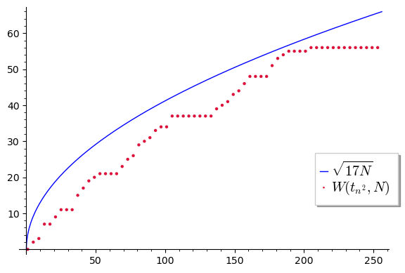
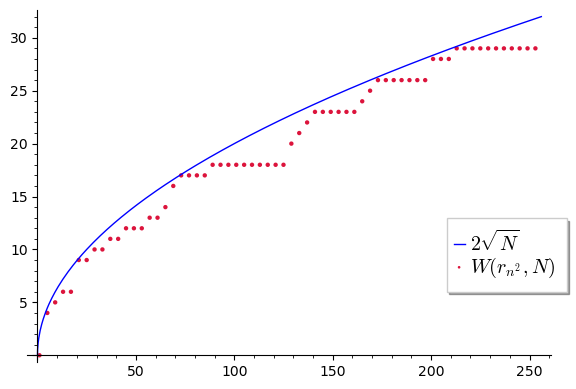
Figure 12: The $N$th well-distribution measure of the Thue-Morse (left) and Rudin-Shapiro (right) sequence along squares.

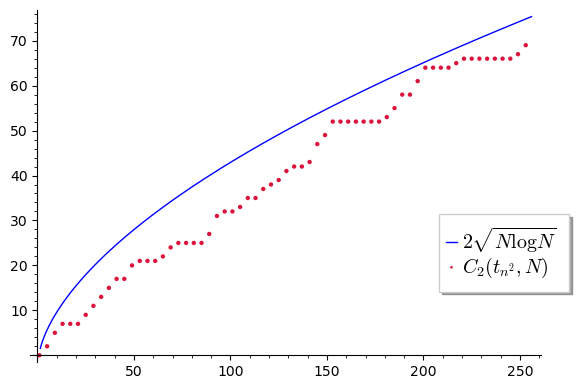
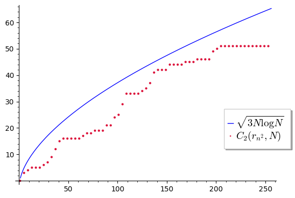
Figure 13: The $N$th second order correlation measure of the Thue-Morse (left) and Rudin-Shapiro (right) sequence along squares.

Problem 3.

For fixed $k=2,3,\ldots$ show that

$$C_{k}(t_{n^{2}},N)=o(N)\quad\mbox{and}\quad C_{k}(r_{n^{2}},N)=o(N).$$

Mauduit and Rivat [61] showed that

$$\left|\sum_{n=0}^{N-1}(-1)^{r_{n^{2}}}z^{n}\right|=O\left(N^{1-\eta}\right),\quad|z|=1,\quad\mbox{for some $\eta>0$},$$

which, together with (5.3), gives a bound on $W(r_{n^{2}},N)$ of the same order of magnitude. More precisely, [61] deals with the more general case of binary pattern sequences $(p_{n})$ defined by (2.13) with either the all one pattern of length $k\geq 2$, that is, $a=2^{k}-1$, or the patterns $10\ldots 01$ of length $k\geq 3$, that is, $a=2^{k-1}+1$, and the constants depend on $k$. For the Thue-Morse sequence along squares $(t_{n^{2}})$ one can easily derive a nontrivial bound on

$$\left|\sum_{n=0}^{N-1}(-1)^{t_{n^{2}}}z^{n}\right|,\quad|z|=1,$$

and thus on $W(t_{n^{2}},N)$ since the proof of [58, Théorème 1] for $z=1$ works also for $z\neq 1$ since after applying a variant of the van der Corput inequality, [58, Lemma 15], we get an expression which does not depend on the variable $z$ anymore, that is, the same expression as for $z=1$.

Theorem 4.1 in Section 4 above shows that the Thue-Morse sequence has maximum order complexity $M(t_{n},N)$ of order of magnitude $N$. Although a large maximum order complexity is desired it should be not too large since otherwise the correlation measure of order $2$ is large. Namely, we have

$$C_{2}(s_{n},N)\geq M(s_{n},N)-1$$ (5.6)

since by [48, Proposition 3.1] there exist $0\leq n_{1}<n_{2}\leq N-M(s_{n},N)-1$ with

$$s_{n_{1}+i}=s_{n_{2}+i},\quad i=0,\ldots,M(s_{n},N)-2,\quad\mbox{but }s_{n_{1}+M(s_{n},N)-1}\neq s_{n_{2}+M(s_{n},N)-1}$$

and thus

$$M(s_{n},N)-1=\sum_{i=0}^{M(s_{n},N)-2}(-1)^{s_{n_{1}+i}+s_{n_{2}+i}}\leq C_{2}(s_{n},N).$$

Combining (4.2) and (5.6) we get for the Thue-Morse sequence

$$C_{2}(t_{n},N)\geq\frac{N}{5},\quad N\geq 4,$$

which further improves the constant in (5.4). Combining (4.3) and (5.6) recovers (5.5). The correlation measure of order $2$ with bounded lags of some generalizations of the Rudin-Shapiro sequence has recently been studied in [56].

In contrast to the Thue-Morse und Rudin-Shapiro sequence, the well-distribution measure of some other binary automatic sequences is very large. For example, the Baum-Sweet sequence $(b_{n})$, the characteristic sequence $(c_{n})$ of the sums of three squares, the paper-folding sequence $(v_{n})$ and the apwenian sequence $(w_{n})$ defined by (2.10) are very unbalanced and thus have all well-distribution measure of order of magnitude $N$. However, it seems to be interesting to study the well-distribution measure for arbitrary apwenian sequences. For the Rudin-Shapiro like sequence $(\ell_{n})$ defined by (2.6) Lafrance, Rampersad and Yee [51] proved

$$\liminf_{N\rightarrow\infty}\frac{\sum_{n=0}^{N-1}(-1)^{\ell_{n}}}{\sqrt{N}}=\frac{\sqrt{3}}{3}\quad\mbox{and}\quad\limsup_{N\rightarrow\infty}\frac{\sum_{n=0}^{N-1}(-1)^{\ell_{n}}}{\sqrt{N}}=\sqrt{2}.$$

However, a bound on $W(\ell_{n},N)$ is not known and in contrast to (5.2) for the Rudin-Shapiro sequence $(r_{n})$, for $(\ell_{n})$ the absolute values

$$\left|\sum_{n=0}^{N-1}(-1)^{\ell_{n}}z^{n}\right|$$

can be of much larger order of magnitude than $\sqrt{N}$ for some $z$ with $|z|=1$, see [3, Theorem 2] as well as [16].

Finally, we remark that the result of Theorem 5.6 provides an estimate on the state complexity of sequences in terms of the correlation measure of order $2$.

Definition 5.3.

Let $k\geq 2$. Then the $N$th state complexity $SC_{k}(s_{n},N)$ of a sequence $(s_{n})$ over $\mathbb{F}_{2}$ is the minimum of the number of states of any finite $k$-automaton which generates the first $N$ sequence elements.

Corollary 5.7.

Let $(s_{n})$ be a binary sequence. Then for all $k\geq 2$ we have

$$SC_{k}(s_{n},N)\geq\frac{N}{k\cdot C_{2}(s_{n},N)}-1\quad\text{for }N\geq 3.$$

6 Expansion complexity

Theorem 3.2 indicates that automatic sequences possess good properties in terms of the linear complexity profile. However, the results of Section 5 show that these sequences have a serious lack of pseudorandomness. Diem [25] showed that these sequences are not just statistically auto-correlated, but are completely predictable from a relatively short initial segment. He introduced the notion of expansion complexity to turn such security flaw into a quantitative form.

Definition 6.1.

Let $(s_{n})$ be a sequence over $\mathbb{F}_{q}$ with generating function

$$G(x)=\sum_{n=0}^{\infty}s_{n}x^{n}\in\mathbb{F}_{q}\llbracket x\rrbracket.$$

For a positive integer $N$, the $N$th expansion complexity $E(s_{n},N)$ of $(s_{n})$ is $E(s_{n},N)=0$ if $s_{0}=\dots=s_{N-1}=0$ and otherwise the least total degree of a non-zero polynomial $h(x,y)\in\mathbb{F}_{q}[x,y]$ such that

$$h(x,G(x))\equiv 0\bmod x^{N}.$$ (6.1)

The sequence $(E(s_{n},N))_{N=1}^{\infty}$ is called expansion complexity profile of $(s_{n})$ and

$$E(s_{n})=\sup_{N\geq 1}E(s_{n},N)$$

is the expansion complexity of $(s_{n})$.

By Christol’s Theorem 2.1, a sequence is automatic if and only if its expansion complexity is finite. For example, we have for the Thue-Morse sequence $(t_{n})$, the Rudin-Shapiro sequence $(r_{n})$, the $p$-ary pattern sequence $(p_{n})$, the Baum-Sweet sequence $(b_{n})$, the Rudin-Shapiro like sequence $(\ell_{n})$ and the characteristic sequence $(c_{n})$ of sums of three squares that

$$E(t_{n})=5,\quad E(r_{n})=7,\quad E(p_{n})\leq p^{\ell}+2p-1,\quad E(b_{n})=3,\quad E(\ell_{n})\leq 12$$

$$E(c_{n})\leq 12,\quad E(v_{n})=6\quad\mbox{and}\quad E(w_{n})=4,$$

which follows from (2.11), (2.12), (2.13), (2.14), (2.15), (2.16), (2.17) and (2.18). The equalities follow from the fact that there is no lower degree polynomial with such property since $h(x,y)$ is irreducible in these cases, see [25, Proposition 4].

Diem showed [25] that if a sequence has small expansion complexity, then long parts of such sequences can be computed efficiently from short ones. We summarize his results.

Theorem 6.1.

Let $(s_{n})$ be a sequence over $\mathbb{F}_{q}$ with expansion complexity $E(s_{n})=d$. From the first $d^{2}$ elements, one can compute an irreducible polynomial $h(x,y)\in\mathbb{F}_{q}[x,y]$ of degree $\deg h\leq d$ with $h(x,G(x))=0$ in polynomial time in $d\cdot\log q$.

Moreover, an initial segment of the sequence of length $M>N$ can be determined from $h$ and the $d^{2}$ initial values in polynomial time in $d\cdot\log q$ and in linear time in $M$.

Theorem 6.1 shows that automatic sequences have a strong non-randomness property. The expansion complexity profile is defined to capture such non-randomness property locally, that is for initial segments of sequences.

For the $N$th expansion complexity, we have the trivial bound $E(s_{n},N)\leq N-1$ realized by the polynomial

$$h(x,y)=y-\sum_{n=0}^{N-1}s_{n}x^{n}.$$

Moreover, one can show the stronger upper bound

$$\binom{E(s_{n},N)+1}{2}\leq N,$$ (6.2)

which holds for all sequence $(s_{n})$ and all $N\geq 1$, see [41, Theorem 1].

The $N$th expansion complexity of random sequences is concentrated to its upper bound (6.2), see [40, Theorem 2].

Theorem 6.2.

We have

$$\liminf_{N\rightarrow\infty}\frac{E(s_{n},N)}{\sqrt{N}}\geq\frac{\sqrt{2}}{2},$$

with probability one with respect to the probability measure (3.1).

One can estimate the $N$th expansion complexity $E(s_{n},N)$ in terms of the $N$th linear complexity $L(s_{n},N)$, see [65, Theorem 3].

Theorem 6.3.

Let $(s_{n})$ be a sequence over $\mathbb{F}_{q}$ and let $G(x)$ bet its generating function. For $N\geq 2$, assume, that

$$G(x)\not\equiv 0\bmod x^{N}.$$

Let $L_{N}=L(s_{n},N)$ be the $N$th linear complexity and let

$$\sum_{\ell=t_{N}}^{L_{N}}c_{\ell}s_{i+\ell}=0,\quad 0\leq i\leq N-L_{N}-1,$$

be a shortest linear recurrence for the first $N$ terms of $(s_{n})$, where $c_{L_{N}}=1$ and $c_{t_{N}}\neq 0$. Then

$$E(s_{n},N)\geq\left\{\begin{array}[]{ll}L_{N}-t_{N}+1&\mbox{for }N>(L_{N}-t_{N})(L_{N}-\min\{1,t_{N}-1\}),\\ \left\lceil\frac{N}{L_{N}-\min\{1,t_{N}-1\}}\right\rceil&\mbox{otherwise,}\end{array}\right.$$

and

$$E(s_{n},N)\leq\min\{L_{N}+\max\{-1,-t_{N}+1\},N-L_{N}+2\}.$$

The result formulates in a qualitative way that very large $N$th linear complexity, that is $N$th linear complexity close to $N$, is a non-randomness property. Moreover, it enables us to estimate the $N$th expansion complexity from below if the $N$th linear complexity is not too close to either $0$ or $N$ (in a logarithmic scale), say, of order of magnitude $\sqrt{N}$.

We refer to [65, 45] for applications of Theorem 6.3 for estimating the $N$th expansion complexity of certain sequences.

Certain subsequences of automatic sequences, say, the Thue-Morse and Rudin-Shapiro sequences along squares are not automatic, see Section 7 below, and thus have unbounded expansion complexity profile. However, their growth rates are not known. For example, one can study further the Thue-Morse and Rudin-Shapiro sequence along squares.

Problem 4.

Estimate the expansion complexity profiles of the subsequences $(t_{n^{2}})$ and $(r_{n^{2}})$ of the Thue-Morse and Rudin-Shapiro sequence along squares.

Figure 14 suggests $E(t_{n^{2}},N)$ and $E(r_{n^{2}},N)$ are both of order of magnitude $\sqrt{N}$.

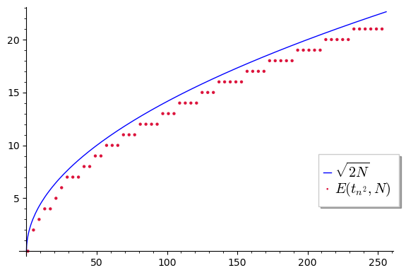
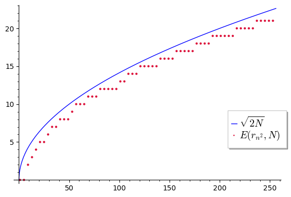
Figure 14: The $N$th expansion complexity of the Thue-Morse (left) and Rudin-Shapiro (right) sequence along squares.

Finally, we remark that in order to use the full strength of Theorem 6.1 for inferring sequence elements, one needs to require the irreducibly of the polynomial $h(x,y)$ in (6.1). In [40, 41], the authors studied this variant of the $N$th expansion complexity and the relation between these two complexity measures.

7 Subword complexity and normality

The results of Section 5 show that many automatic sequences, including Thue-Morse and Rudin-Shapiro sequence, are balanced, that is, the frequencies of the symbols are close to the expected values. However, the frequencies of longer patterns are far from uniform. This phenomenon can be made precise by the notion of subword complexity.

Definition 7.1.

For a sequence $(s_{n})$ over the alphabet $\Delta$ the subword complexity $p(s_{n},k)$ is the number of distinct subsequences of length $k$.

Trivially we have $1\leq p(s_{n},k)\leq|\Delta|^{k}$ and for ultimately periodic sequences we have $p(s_{n},k)=O(1)$.

By [7, Corollary 10.3.2] the subword complexity $p(s_{n},k)$ of automatic sequences $(s_{n})$ is of order of magnitude $k$.

Theorem 7.1.

If $(s_{n})$ is an automatic sequence that is not ultimately periodic, then we have

$$p(s_{n},k)=\Theta(k).$$

For the Thue-Morse sequence $(t_{n})$, the exact value of its subword complexity $p(t_{n},k)$ was independently determined by Brlek [13, Proposition 4.4] and by de Luca and Varricchio [24, Proposition 4.4], see also [7, Exercise 10.11.10]. De Luca and Varricchio [24, Property 3.3] also showed that patterns such as $000$ and $111$ do not appear in the Thue-Morse sequence and more general the following result.

Theorem 7.2.

The Thue-Morse sequence is cube-free, that is, no pattern of the form $www$ with $w\in\{0,1\}^{k}$ for some $k\geq 1$ appears in the sequence.

The papers [13, 24] contain also several other results on the non-existence of certain patterns in the Thue-Morse sequence.

The subword complexity and the correlation measure of order $\ell$ are related by the following result of Cassaigne et al. [15, Theorem 6].

Theorem 7.3.

If for some positive integers $k$ and $N$

$$C_{\ell}(s_{n},N)\leq\frac{N}{2^{2k+1}},\quad\ell=1,2,\ldots,k,$$

then

$$p(s_{n},k)=2^{k}.$$

For automatic sequences we can have $p(s_{n},k)=2^{k}$ only for finitely many $k$ since $p(s_{n},k)=\Theta(k)$. However, certain subsequences of automatic squences are normal, that is, all patterns appear in the sequence with the expected frequencies. More formally, a sequence $(s_{n})$ is called normal if for any fixed length $k$ and any pattern $\mathbf{e}\in\Delta^{k}$

$$N_{k}(s_{n},\mathbf{e},N)=\frac{\#\{0\leq n<N:(s_{n},s_{n+1},\ldots,s_{n+k-1})=\mathbf{e}\}}{N}\rightarrow\frac{1}{|\Delta|^{k}}\quad\text{as }N\rightarrow\infty.$$

Drmota et al. [32] and Müllner [71] proved the normality of the Thue-Morse and the Rudin-Shapiro sequences along squares, that is

$$\lim_{N\rightarrow\infty}N_{k}(t_{n^{2}},\mathbf{e},N)=2^{-k}\quad\text{and}\quad\lim_{N\rightarrow\infty}N_{k}(t_{n^{2}},\mathbf{e},N)=2^{-k}$$ (7.1)

for any $\mathbf{e}\in\{0,1\}^{k}$. The main tool to obtain the results (7.1) is to prove estimates on the sums

$$\sum_{n<N}(-1)^{e_{0}t_{n^{2}}+\dots+e_{k-1}t_{(n+k-1)^{2}}}\quad\text{and}\quad\sum_{n<N}(-1)^{e_{0}r_{n^{2}}+\dots+e_{k-1}r_{(n+k-1)^{2}}}$$

for any $e_{0},\dots,e_{k-1}\in\{0,1\}$. These sums can be estimated via a Fourier analytic method of Mauduit and Rivat which has its origin in [58, 59]. For more details we refer to the survey [31] of Drmota and the original papers [32, 71].

In particular, the normality results (7.1) yield the the subword complexities

$$p(t_{n^{2}},k)=p(r_{n^{2}},k)=2^{k}.$$ (7.2)

It is conjectured but not proved yet that the subsequences of the Thue-Morse sequence $(t_{f(n)})$ and Rudin-Shapiro sequence $(r_{f(n)})$ along any polynomial $f$ of degree $d\geq 3$ are normal, see [32, Conjecture 1]. Even the weaker problem of determining the frequency of $0$ and $1$ in the subsequences $(t_{f(n)})$ and $(r_{f(n)})$ along any polynomial $f(x)$ of degree $d\geq 3$ with $f(\mathbb{N}_{0})\subset\mathbb{N}_{0}$ seems to be very intricate, see [32, above Conjecture 1].

Problem 5.

Show that the subsequences of Thue-Morse and Rudin-Shapiro sequence along cubes, bi-squares, …, any polynomial values for a polynomial of degree at least $3$ are normal.

However, Moshe [69] proved the following lower bound on the subword complexity of $(t_{f(n)})$,

$$p(t_{f(n)},k)\geq 2^{k/2^{d-2}}.$$ (7.3)

Stoll [88, 90] showed that the number of zeros (resp. ones) among the first $N$ sequence elements of both, $(t_{f(n)})$ and $(r_{f(n)})$, is at least of order of magnitude $N^{4/(3d+1)}$, $d\geq 3$. For subsequences $(z_{f(n)})$ of the Zeckendorf sum of digits sequence $(z_{n})$ defined by (4.4) the numbers of zeros and ones among the first $N$ sequence elements are both lower bounded by $N^{4/(6d+1)}$, see Stoll [89].

Müllner and Spiegelhofer [72, 86] addressed the normality problem for the Thue-Morse sequence along the Piateski-Shapiro sequence $\lfloor n^{c}\rfloor$ for $1<c<3/2$. Moreover, it is asymptotically balanced (or simply normal)[87, Theorem 1.2] for $1<c<2$. For results on the Thue-Morse and Rudin-Shapiro sequence along primes see [11, 12, 59, 60] and references therein. In particular, the Thue-Morse sequence $(t_{p})$ along primes is balanced, see Mauduit and Rivat [59]. However, it is not known whether $(t_{f(p)})_{p}$ is normal for any nonconstant polynomial $f$.

From Theorem 7.1 and (7.2) we know that $(t_{n^{2}})$ and $(r_{n^{2}})$ are not automatic and by Theorem 2.1 these subsequences are, in contrast to the original sequence, not of bounded expansion complexity, that is,

$$\lim\limits_{N\rightarrow\infty}E(t_{n^{2}},N)=\lim\limits_{N\rightarrow\infty}E(r_{n^{2}},N)=\infty.$$

Theorem 7.1 combined with (7.3) implies that $(t_{f(n)})$ is not automatic and

$$\lim\limits_{N\rightarrow\infty}E(t_{f(n)})=\infty$$

for any polynomial of degree at least $2$ with $f(\mathbb{N}_{0})\subset\mathbb{N}_{0}$. Note that it was shown in [2] that $(t_{f(n)})$ is not $2^{r}$-automatic and in [5] that $(r_{f(n)})$ is not $2^{r}$-automatic and thus we also have

$$\lim\limits_{N\rightarrow\infty}E(r_{f(n)})=\infty.$$

Subsequences of the Thue-Morse sequence along geometric sequences such as $(t_{3^{n}})$ seem to be even more difficult to analyze. For example, Lagarias [52, Conjecture 1.12] conjectured that each pattern appears at least once in $(t_{3^{n}})$. For other related results see[33, 50].

For more details on the normality of automatic sequences and their subsequences we refer to [31].

8 Analogs for finite fields

An analog for finite fields of the problem on the distribution of automatic sequences and their subsequences was introduced by Dartyge and Sárközy [22]. It has been further investigated in [21, 55, 94, 95, 57], see also [26, 37, 96, 20, 77].

In the finite field setting some problems can be solved although the analog for integers seems to be out of reach including the normality problem for the analog of the Thue-Morse sequence and the frequency problem for the analog of the Rudin-Shapiro sequence both along polynomials. Hence, these analogs for finite fields are further attractive sources of pseudorandomness.

For a prime $p$ and $q=p^{r}$ with $r\geq 2$ let $(\beta_{1},\ldots,\beta_{r})$ be an ordered basis of $\mathbb{F}_{q}$ over $\mathbb{F}_{p}$. Then one can write all elements $\xi\in\mathbb{F}_{q}$ as

$$\xi=\sum_{i=1}^{r}x_{i}\beta_{i},\quad x_{1},\dots,x_{r}\in\mathbb{F}_{p}.$$ (8.1)

It is natural to consider the coefficients $x_{1},\dots,x_{r}$ as digits with respect to the basis $(\beta_{1},\dots,\beta_{r})$. Then, in analogy to the Thue-Morse and Rudin-Shapiro sequence satisfying (2.5) we define the Thue-Morse function

$$T\left(\sum_{i=1}^{r}x_{i}\beta_{i}\right)=\sum_{i=1}^{r}x_{i},\quad x_{1},\ldots,x_{r}\in\mathbb{F}_{p},$$

and Rudin-Shapiro function

$$R\left(\sum_{i=1}^{r}x_{i}\beta_{i}\right)=\sum_{i=1}^{r-1}x_{i}x_{i+1},\quad x_{1},\ldots,x_{r}\in\mathbb{F}_{p},$$

on $\mathbb{F}_{q}$.

Dartyge and Sárközy [22] studied the balance of the Thue-Morse function along polynomial values. They derived results using the Weil bound [54, Theorem 5.38] on additive character sums:

Lemma 8.1.

Let $f\in\mathbb{F}_{q}[x]$ be of degree $d\geq 1$ with $\gcd(d,q)=1$ and $\psi$ be a nontrivial additive character of $\mathbb{F}_{q}$. Then

$$\left|\sum_{\xi\in\mathbb{F}_{q}}\psi(f(\xi))\right|\leq(d-1)\sqrt{q}.$$

Put

$$e(\alpha)=\exp(2\pi i\alpha),\quad\alpha\in\mathbb{R},$$

and note that $\psi(x)=e(T(x)/p)$ is a nontrivial additive character of $\mathbb{F}_{q}$. Then from

$$\sum_{h=0}^{p-1}e\left(\frac{ha}{p}\right)=\left\{\begin{array}[]{cc}0,&a\neq 0,\\ p,&a=0,\end{array}\right.\quad a\in\mathbb{F}_{p},$$

we get

$$\#\{\xi\in\mathbb{F}_{q}:T(f(\xi))=c\}=\frac{1}{p}\sum_{h=0}^{p-1}\sum_{\xi\in\mathbb{F}_{q}}\psi\left(hf(\xi)\right)e\left(\frac{-hc}{p}\right).$$

The contribution of $h=0$ is trivially $p^{r-1}$, which is the expected number of solutions. The other terms for $h\neq 0$ contribute to the error term and can be bounded by Lemma 8.1. We immediately get [22, Theorem 1.2]:

Theorem 8.2.

Let $f\in\mathbb{F}_{q}[x]$ be of degree $d$ with $\gcd(d,q)=1$. Then for all $c\in\mathbb{F}_{p}$, we have

$$\big{|}\#\{\xi\in\mathbb{F}_{q}:T(f(\xi))=c\}-p^{r-1}\big{|}\leq(d-1)p^{r/2}.$$

Later Dartyge, Mérai and Winterhof [21] investigated this problem for the Rudin-Shapiro function. The main difference between the two problems is that the Rudin-Shapiro function is not a linear map contrary to the Thue-Morse function. Standard character sum techniques fail in this situation. Namely, consider $R(f(\xi))$ with $\xi$ having the form (8.1) as a polynomial in the $r$ variables $x_{1},\dots,x_{r}$. Then using Lemma 8.1 for one coordinate $x_{i}$ one gets an error term larger than the main term. Stronger results in higher dimension such as the Deligne bound [23, Théorème 8.4] also cannot be applied as it needs some more technically intricate conditions which are not satisfied in our situation. However, sacrificing the explicit dependence of the degree $d$, one can use an affine version of the Hooley-Katz Theorem, see [46] or [70, Theorem 7.1.14].

First recall that the (affine) singular locus ${\mathcal{L}}(F)$ of a polynomial $F\in\mathbb{F}_{p}[x_{1},\dots,x_{r}]$ is the set of common zeros in $\overline{\mathbb{F}_{p}}^{r}$ of the polynomials

$$F,\frac{\partial F}{\partial x_{1}},\ldots,\frac{\partial F}{\partial x_{r}}.$$

We also recall that the dimension of ${\mathcal{L}}(F)$ is the largest $d$ for which there exist $1\leq i_{1}<i_{2}<\ldots<i_{d}\leq r$ such that there is no nonzero polynomial $P$ in $d$ variables with $P(y_{i_{1}},\ldots,y_{i_{d}})=0$ for all $(y_{1},\ldots,y_{r})\in{\mathcal{L}}(F)$, see [19, Corollary 9.5.4].

Lemma 8.3.

Let $Q\in\mathbb{F}_{p}[x_{1},\dots,x_{r}]$ be of degree $d\geq 1$ such that the dimensions of the singular loci of $Q$ and its homogeneous part $Q_{d}$ of degree $d$ satisfy

$$\max\{\dim({\mathcal{L}}(Q)),\dim({\mathcal{L}}(Q_{d}))-1\}\leq s.$$

Then the number $N$ of zeros of $Q$ in $\mathbb{F}_{p}^{r}$ satisfies

$$\left|N-p^{r-1}\right|\leq C_{d,r}p^{(r+s)/2},$$

where $C_{d,r}$ is a constant depending only on $d$ and $r$.

Then using Lemma 8.3, one can show that the Rudin-Shapiro function is also asymptotically balanced on polynomial values, see [21, Theorem 1].

Theorem 8.4.

Let $f\in\mathbb{F}_{q}[x]$ be of degree $d$ with $\gcd(d,q)=1$. Then for all $c\in\mathbb{F}_{p}$, we have

$$\big{|}\#\{\xi\in\mathbb{F}_{q}:R(f(\xi))=c\}-p^{r-1}\big{|}\leq C_{d,r}p^{(3r+1)/4},$$

where the constant $C_{d,r}$ depends only on the degree $d$ of $f$ and $r$.

Theorem 8.4 is nontrivial if $r$ is fixed and $p\rightarrow\infty$. Contrary to Theorem 8.2, nothing is known for the dual situation.

Problem 6.

For fixed prime $p$ show that if $r$ is large enough, then the Rudin-Shapiro function along polynomial values is balanced possibly under some natural restrictions on the polynomial.

Analogously to the normality results of Section 7, Makhul and Winterhof [55] obtained results on the normality of the Thue-Morse function along polynomial values. For sake of simplicity we state the case when the polynomial $f$ has degree $d$ smaller than the characteristic $p$, [55, Corollary 1].

Theorem 8.5.

Assume $1\leq d<p$ and $s\leq d$. For any polynomial $f\in\mathbb{F}_{q}[x]$ of degree $d$ and any pairwise distinct $\alpha_{1},\dots,\alpha_{s}\in\mathbb{F}_{q}$ and any $c_{1},\dots,c_{s}\in\mathbb{F}_{p}$ we have

$$\big{|}\#\{\xi\in\mathbb{F}_{q}:T(f(\xi+\alpha_{i}))=c_{i},1\leq i\leq s\}-p^{r-s}\big{|}\leq(d-1)p^{r/2}.$$

Note that the restriction $s\leq d$ is natural and counterexamples for $s>d$ are easy to construct.

The case of the Rudin-Shapiro function is much more intricate.

Problem 7.

Study the normality of the Rudin-Shapiro function at $f(x)$. Namely, show that

$$\frac{\#\{\xi\in\mathbb{F}_{q}:R(f(\xi+\alpha_{i}))=c_{i},1\leq i\leq s\}}{p^{r-s}}\rightarrow 1\quad\text{as }p\rightarrow\infty$$

for some $s\geq 2$ and any $f\in\mathbb{F}_{q}[x]$ of fixed degree.

Of course, this problem is also open for fixed $p$ and $r\rightarrow\infty$ even in the simplest case $s=1$, see Problem 6.

It is natural to define the Rudin-Shapiro function on the polynomial ring $\mathbb{F}_{p}[t]$ by assigning the coefficients of the polynomial $f(t)\in\mathbb{F}_{p}[t]$ to $(x_{1},\dots,x_{r})$, that is,

$$R(t^{r}+x_{1}t^{r-1}+\dots+x_{r})=\sum_{i=1}^{r-1}x_{i}x_{i+1},$$

for $x_{1},\dots,x_{r}\in\mathbb{F}_{p}$.

Analogously to the result of Mauduit and Rivat [60] on the Rudin-Shapiro sequence along prime numbers, it is natural to investigate the balance and the normality of the Rudin-Shapiro function along irreducible polynomials. As the number of monic irreducible polynomials of degree $r$ is $p^{r}/r+o(p^{r})$, see for example [54, Theorem 3.25], we expect that the frequency of each element $c$ is $\frac{p^{r-1}}{r}+o(p^{r-1})$. For $r=2$ and fixed $c\in\mathbb{F}_{p}$ we have to count the number of $x_{2}\in\mathbb{F}_{p}^{*}$ such that $t^{2}+x_{2}^{-1}ct+x_{2}$ is irreducible over $\mathbb{F}_{p}$ or equivalently the discriminant $x_{2}^{-2}c^{2}-4x_{2}$ is a quadratic non-residue modulo $p$. This number is

$$\frac{1}{2}\sum_{x_{2}\in\mathbb{F}_{p}^{*}}\left(1-\left(\frac{c^{2}-4x_{2}^{3}}{p}\right)\right)=\left\{\begin{array}[]{cc}\frac{p-1}{2},&c=0,\\ \frac{p-1}{2}+O(p^{1/2}),&c\neq 0,\end{array}\right.$$

by the Weil bound for multiplicative character sums [54, Theorem 5.41], where $\left(\frac{.}{.}\right)$ is the Legendre symbol.

Problem 8.

Prove that for all $c\in\mathbb{F}_{p}$ and $r\geq 3$ we have

$$\lim_{p\rightarrow\infty}\frac{\#\{f\in\mathbb{F}_{p}[t]:\deg f=r,f\text{ monic and irreducible over $\mathbb{F}_{p}$},R(f)=c\}}{p^{r-1}}=\frac{1}{r}.$$

We remark that one can define the Thue-Morse function by

$$T(f)=T(t^{r}+x_{1}t^{r-1}+\ldots+x_{r})=x_{1}+\ldots+x_{r}=f(1)-1.$$

Note that for irreducible polynomials $f(x)$ we have $T(f)\neq-1$ and for $c\neq-1$ the number of monic irreducible polynomials of degree $r=2$ with $T(f)=c$ is

$$\frac{1}{2}\sum_{u\in\mathbb{F}_{p}\atop u^{2}\neq c+1}\left(1-\left(\frac{u^{2}-c-1}{p}\right)\right)=\frac{p-\left(\frac{c+1}{p}\right)}{2},$$

where we used a well-known result on sums of Legendre symbols of quadratic polynomials, see for example [54, Theorem 5.48]. In general, since $f(x)$ is irreducible whenever $f(x-1)$ is irreducible we have to estimate the number $I_{c}$ of monic irreducible polynomials with fixed constant term $c\neq 0$ which satisfies

$$\frac{1}{r}\left(\frac{p^{r}-1}{p-1}-2p^{r/2}\right)\leq I_{c}\leq\frac{p^{r}-1}{r(p-1)},$$

see [14] or [70, Theorem 3.5.9], and we get the desired

$$I_{c}=\frac{p^{r-1}}{r}+o(p^{r-1})$$

for $r\geq 3$ as well.

Moreover, the corresponding normality problem is trivial since for any polynomial $g(x)$ of degree at most $r-1$ the value $T(f+g)=f(1)+g(1)-1$ is uniquely defined by $T(f)=f(1)-1$ and $g(1)$.

For other results on ’digits’ along irreducible polynomials see for example [70, Chapter 3] and [38, 42, 78, 98, 44, 80].

References

- [1] C. Aistleitner, On the limit distribution of the well-distribution measure of random binary sequences. J. Théor. Nombres Bordeaux 25 (2013), no. 2, 245–259.
- [2] J.-P. Allouche, Somme des chiffres et transcendance. Bull. Soc. Math. France 110 (1982), no. 3, 279–285.
- [3] J.-P. Allouche, On a Golay-Shapiro-like sequence. Unif. Distrib. Theory 11 (2016), no. 2, 205–210.
- [4] J.-P. Allouche, G.-N. Han, H. Niederreiter, Perfect linear complexity profile and apwenian sequences. Finite Fields Appl. 68 (2020), 101761, 13 pp.
- [5] J.-P. Allouche, O. Salon, Sous-suites polynomiales de certaines suites automatiques. J. Théor. Nombres Bordeaux 5 (1993), no. 1, 111–121.
- [6] J.-P. Allouche, J. Shallit, The ubiquitous Prouhet-Thue-Morse sequence. Sequences and their applications (Singapore, 1998), 1–16, Springer Ser. Discrete Math. Theor. Comput. Sci., Springer, London, 1999.
- [7] J.-P. Allouche, J. Shallit, Automatic sequences. Theory, applications, generalizations. Cambridge University Press, Cambridge, 2003.
- [8] J.-P. Allouche, J. Shallit, R. Yassawi, How to prove that a sequence is not automatic, Preprint 2021. Available at https://arxiv.org/abs/2104.13072
- [9] N. Alon, Y. Kohayakawa, C. Mauduit, C. G. Moreira, V. Rödl, Measures of pseudorandomness for finite sequences: typical values. Proc. Lond. Math. Soc. (3) 95 (2007), no. 3, 778–812.
- [10] A. Blumer, J. Blumer, A. Ehrenfeucht, D. Haussler, R. McConnell, Linear size finite automata for the set of all subwords of a word: an outline of results. Bul. Eur. Assoc. Theor. Comp. Sci. 21 (1983), 12–20.
- [11] J. Bourgain, Prescribing the binary digits of primes. Israel J. Math. 194 (2013), no. 2, 935–955.
- [12] J. Bourgain, Prescribing the binary digits of primes, II. Israel J. Math. 206 (2015), no. 1, 165–182.
- [13] S. Brlek, Enumeration of factors in the Thue-Morse word. First Montreal Conference on Combinatorics and Computer Science, 1987. Discrete Appl. Math. 24 (1989), no. 1-3, 83–96.
- [14] M. Car, Distribution des polynômes irréductibles dans . Acta Arith. 88 (1999), no. 2, 141–153.
- [15] J. Cassaigne, S. Ferenczi, C. Mauduit, J. Rivat, A. Sárközy, On finite pseudorandom binary sequences. III. The Liouville function. I. Acta Arith. 87 (1999), no. 4, 367–390.
- [16] L. Chan, U. Grimm, Spectrum of a Rudin-Shapiro-like sequence. Adv. in Appl. Math. 87 (2017), 16–23.
- [17] G. Christol, Ensembles presque périodiques -reconnaissables. Theoret. Comput. Sci. 9 (1979), no. 1, 141–145.
- [18] G. Christol, T. Kamae, M. Mendès France, G. Rauzy, Suites algébriques, automates et substitutions. Bull. Soc. Math. France 108 (1980), no. 4, 401–419.
- [19] D. A. Cox, J. Little, D. O’Shea, Ideals, varieties, and algorithms. Undergraduate Texts in Mathematics. Springer, Cham, fourth edition, 2015. An introduction to computational algebraic geometry and commutative algebra.
- [20] C. Dartyge, C. Mauduit, A. Sárközy, Polynomial values and generators with missing digits in finite fields. Funct. Approx. Comment. Math. 52 (2015), no. 1, 65–74.
- [21] C. Dartyge, L. Mérai, A. Winterhof, On the distribution of the Rudin-Shapiro function for finite fields. arxiv:2006.02791.
- [22] C. Dartyge, A. Sárközy, The sum of digits function in finite fields. Proc. Amer. Math. Soc. 141 (2013), no. 12, 4119–4124.
- [23] P. Deligne. La conjecture de Weil. Inst. Hautes Études Sci. Publ. Math., 43 (1974) 273–-307.
- [24] A. de Luca, S. Varricchio, Some combinatorial properties of the Thue-Morse sequence and a problem in semigroups. Theoret. Comput. Sci. 63 (1989), no. 3, 333–348.
- [25] C. Diem, On the use of expansion series for stream ciphers. LMS J. Comput. Math. 15 (2012), 326–340.
- [26] R. Dietmann, C. Elsholtz, I. E. Shparlinski, Prescribing the binary digits of squarefree numbers and quadratic residues. Trans. Amer. Math. Soc. 369 (2017), no. 12, 8369–8388.
- [27] G. Dorfer, Lattice profile and linear complexity profile of pseudorandom number sequences. Finite fields and applications, 69–78, Lecture Notes in Comput. Sci., 2948, Springer, Berlin, 2004.
- [28] G. Dorfer, W. Meidl, A. Winterhof, Counting functions and expected values for the lattice profile at . Finite Fields Appl. 10 (2004), no. 4, 636–652.
- [29] G. Dorfer, A. Winterhof, Lattice structure and linear complexity profile of nonlinear pseudorandom number generators. Appl. Algebra Engrg. Comm. Comput. 13 (2003), no. 6, 499–508.
- [30] G. Dorfer, A. Winterhof, Lattice structure of nonlinear pseudorandom number generators in parts of the period. Monte Carlo and quasi-Monte Carlo methods 2002, 199–211, Springer, Berlin, 2004.
- [31] M. Drmota, Subsequences of automatic sequences and uniform distribution. Uniform distribution and quasi-Monte Carlo methods, 87–104, Radon Ser. Comput. Appl. Math., 15, De Gruyter, Berlin, 2014.
- [32] M. Drmota, C. Mauduit, J. Rivat, Normality along squares. J. Eur. Math. Soc. 21 (2019), no. 2, 507–548.
- [33] T. Dupuy, D. E. Weirich, Bits of in binary, Wieferich primes and a conjecture of Erdős. J. Number Theory 158 (2016), 268–280.
- [34] G. Everest, A. van der Poorten, I. Shparlinski, T. Ward, Recurrence sequences. Mathematical Surveys and Monographs, 104. American Mathematical Society, Providence, RI, 2003.
- [35] N. P. Fogg, Substitutions in dynamics, arithmetics and combinatorics. Edited by V. Berthé, S. Ferenczi, C. Mauduit and A. Siegel. Lecture Notes in Mathematics, 1794. Springer-Verlag, Berlin, 2002.
- [36] E. Fouvry, C. Mauduit, Sommes des chiffres et nombres presque premiers. Math. Ann. 305 (1996), 571–599.
- [37] M. R. Gabdullin, On the squares in the set of elements of a finite field with constraints on the coefficients of its basis expansion. (Russian) Mat. Zametki 100 (2016), no. 6, 807–824; translation in Math. Notes 101 (2017), no. 1–2, 234–249.
- [38] Z. Gao, S. Kuttner, Q. Wang, On enumeration of irreducible polynomials and related objects over a finite field with respect to their trace and norm. Finite Fields Appl. 69 (2021), 101770, 25 pp.
- [39] A. O. Gel’fond, Sur les nombres qui ont des propriétés additives et multiplicatives données. (French) Acta Arith. 13 (1967/68), 259–265.
- [40] D. Gómez-Pérez, L. Mérai, Algebraic dependence in generating functions and expansion complexity. Adv. Math. Commun. 14 (2020) no. 2, 307–318.
- [41] D. Gómez-Pérez, L. Mérai, H. Niederreiter, On the expansion complexity of sequences over finite fields. IEEE Trans. Inform. Theory 64 no. 6 (2018), 4228–4232.
- [42] R. Granger, On the enumeration of irreducible polynomials over with prescribed coefficients. Finite Fields Appl. 57 (2019), 156–229.
- [43] K. Gyarmati, Measures of pseudorandomness. Finite fields and their applications. 43–64, Radon Ser. Comput. Appl. Math., 11, De Gruyter, Berlin, 2013.
- [44] J. Ha, Irreducible polynomials with several prescribed coefficients. Finite Fields Appl. 40 (2016), 10–25.
- [45] R. Hofer, A. Winterhof, Linear complexity and expansion complexity of some number theoretic sequences. Arithmetic of finite fields, 67–74, Lecture Notes in Comput. Sci., 10064, Springer, Cham, 2016.
- [46] C. Hooley, On the number of points on a complete intersection over a finite field. With an appendix by Nicholas M. Katz. J. Number Theory 38 (1991), no. 3, 338–358.
- [47] D. Jamet, P. Popoli, T. Stoll, Maximum order complexity of the sum of digits function in Zeckendorf base and polynomial subsequences, Preprint 2021.
- [48] C. J. A. Jansen, Investigations on nonlinear streamcipher systems: Construction and evaluation methods. Thesis (Dr.)–Technische Universiteit Delft (The Netherlands). ProQuest LLC, Ann Arbor, MI, 1989. 195 pp.
- [49] C. J. A. Jansen, D. E. Boekee, The shortest feedback shift register that can generate a given sequence. Advances in cryptology—CRYPTO ’89 (Santa Barbara, CA, 1989), 90–99, Lecture Notes in Comput. Sci., 435, Springer, New York, 1990.
- [50] H. Kaneko, T. Stoll, On subwords in the base- expansion of polynomial and exponential functions. Integers 18A (2018), Paper No. A11, 11 pp.
- [51] P. Lafrance, N. Rampersad, R. Yee, Some properties of a Rudin-Shapiro-like sequence. Adv. in Appl. Math. 63 (2015), 19–40.
- [52] J. Lagarias, Ternary expansions of powers of . J. Lond. Math. Soc. (2) 79 (2009), no. 3, 562–588.
- [53] P. L’Ecuyer, R. Simard, TestU01: A C Library for Empirical Testing of Random Number Generators. ACM Transactions on Mathematical Software, Vol. 33, article 22, 2007.
- [54] R. Lidl, H. Niederreiter, Finite fields. Second edition. Encyclopedia of Mathematics and its Applications, 20. Cambridge University Press, Cambridge, 1997.
- [55] M. Makhul, A. Winterhof, Normality of the Thue-Morse function for finite fields along polynomial values. Preprint 2021.
- [56] I. Marcovici, T. Stoll, P.-A. Tahay, Discrete correlations of order of generalized Golay-Shapiro sequences: A combinatorial approach. Integers 21 (2021), Paper No. A45, 21 pp.
- [57] S. Mattheus, Trace of products in finite fields from a combinatorial point of view. SIAM J. Discrete Math. 33 (2019), no. 4, 2126–2139.
- [58] C. Mauduit, J. Rivat, La somme des chiffres des carrés. Acta Math. 203 (2009), no. 1, 107–148.
- [59] C. Mauduit, J. Rivat, Sur un probléme de Gelfond: la somme des chiffres des nombres premiers. Ann. of Math. (2) 171 (2010), no. 3, 1591–1646.
- [60] C. Mauduit, J. Rivat, Prime numbers along Rudin-Shapiro sequences. J. Eur. Math. Soc. (JEMS) 17 (2015), no. 10, 2595–2642.
- [61] C. Mauduit, J. Rivat, Rudin-Shapiro sequences along squares. Trans. Amer. Math. Soc. 370 (2018), no. 11, 7899–7921.
- [62] C. Mauduit, A. Sárközy, On finite pseudorandom binary sequences. I. Measure of pseudorandomness, the Legendre symbol. Acta Arith. 82 (1997), no. 4, 365–377.
- [63] C. Mauduit, A. Sárközy, On finite pseudorandom binary sequences. II. The Champernowne, Rudin-Shapiro, and Thue-Morse sequences, a further construction. J. Number Theory 73 (1998), no. 2, 256–276.
- [64] C. Mauduit, A. Sárközy, On the measures of pseudorandomness of binary sequences. Discrete Math. 271 (2003), no. 1-3, 195–207.
- [65] L. Mérai, H. Niederreiter, A. Winterhof, Expansion complexity and linear complexity of sequences over finite fields. Cryptogr. Commun. 9 (2017), no. 4, 501–509.
- [66] L. Mérai, J. Rivat, A. Sárközy, The measures of pseudorandomness and the NIST tests. Number-theoretic methods in cryptology, 197–216, Lecture Notes in Comput. Sci., 10737, Springer, Cham, 2018.
- [67] L. Mérai, A. Winterhof, On the pseudorandomness of automatic sequences. Cryptogr. Commun. 10 (2018), no. 6, 1013–1022.
- [68] L. Mérai, A. Winterhof, On the th linear complexity of automatic sequences. J. Number Theory 187 (2018), 415–429.
- [69] Y. Moshe, On the subword complexity of Thue-Morse polynomial extractions. Theoret. Comput. Sci. 389 (2007), no. 1-2, 318–329.
- [70] G. L. Mullen, D. Panario (eds.), Handbook of finite fields. Discrete Mathematics and its Applications (Boca Raton). CRC Press, Boca Raton, FL, 2013.
- [71] C. Müllner, The Rudin-Shapiro sequence and similar sequences are normal along squares. Canad. J. Math. 70 (2018), no. 5, 1096–1129.
- [72] C. Müllner, L. Spiegelhofer, Normality of the Thue-Morse sequence along Piatetski-Shapiro sequences, II. Israel J. Math. 220 (2017), no. 2, 691–738.
- [73] H. Niederreiter, Sequences with almost perfect linear complexity profile. Advances in cryptology-EUROCRYPT ’87 (D. Chaum and W. L. Price, Eds.), Lecture Notes in Computer Science, Vol. 304, pp. 37–51, Springer-Verlag, Berlin/Heidelberg/New York, 1988
- [74] H. Niederreiter, The probabilistic theory of linear complexity. Advances in Cryptology – EUROCRYPT ’88 (C. G. Günther, ed.) Lecture Notes in Computer Science, Vol. 330, pp. 191–209, Springer, Berlin, 1988.
- [75] H. Niederreiter, Linear complexity and related complexity measures for sequences. Progress in Cryptology—INDOCRYPT 2003, 1–17, Lecture Notes in Comput. Sci. 2904, Springer, Berlin, 2003.
- [76] H. Niederreiter, A. Winterhof, Applied number theory. Springer, Cham, 2015.
- [77] A. Ostafe, Polynomial values in affine subspaces of finite fields. J. Anal. Math. 138 (2019), no. 1, 49–81.
- [78] P. Pollack, Irreducible polynomials with several prescribed coefficients. Finite Fields Appl. 22 (2013), 70–78.
- [79] P. Popoli, On the maximum order complexity of Thue-Morse and Rudin-Shapiro sequences along polynomial values. Unif. Distrib. Theory 15 (2020), no. 2, 9–22.
- [80] S. Porritt, Irreducible polynomials over a finite field with restricted coefficients. Canad. Math. Bull. 62 (2019), no. 2, 429–439.
- [81] W. Rudin, Some theorems on Fourier coefficients. Proc. Amer. Math. Soc. 10 (1959) 855–859.
- [82] A. Rukhin et al., NIST Special Publication 800-22, Revision 1.a, A Statistical Test Suite for Random and Pseudorandom Number Generators for Cryptographic Applications, https://www.nist.gov/publications/ statistical-test-suite-random-and-pseudorandom-number-generators-cryptographic
- [83] K.-U. Schmidt, The correlation measures of finite sequences: limiting distributions and minimum values. Trans. Amer. Math. Soc. 369 (2017), no. 1, 429–446.
- [84] H. S. Shapiro, Extremal problems for polynomials and power series. Master’s thesis, MIT, 1952.
- [85] I. Shparlinski, Cryptographic applications of analytic number theory. Complexity lower bounds and pseudorandomness. Progress in Computer Science and Applied Logic, 22. Birkhäuser Verlag, Basel, 2003.
- [86] L. Spiegelhofer, Normality of the Thue-Morse sequence along Piatetski-Shapiro sequences. Q. J. Math. 66 (2015), no. 4, 1127–1138.
- [87] L. Spiegelhofer, The level of distribution of the Thue-Morse sequence. Compos. Math. 156 (2020), no. 12, 2560–2587.
- [88] T. Stoll, The sum of digits of polynomial values in arithmetic progressions. Funct. Approx. Comment. Math. 47 (2012), part 2, 233–239.
- [89] T. Stoll, Combinatorial constructions for the Zeckendorf sum of digits of polynomial values. Ramanujan J. 32 (2013), no. 2, 227–243.
- [90] T. Stoll, On digital blocks of polynomial values and extractions in the Rudin-Shapiro sequence. RAIRO Theor. Inform. Appl. 50 (2016), no. 1, 93–99.
- [91] Z. Sun, A. Winterhof, On the maximum order complexity of subsequences of the Thue-Morse and Rudin-Shapiro sequence along squares. Int. J. Comput. Math. Comput. Syst. Theory 4 (2019), no. 1, 30–36.
- [92] Z. Sun, A. Winterhof, On the maximum order complexity of the Thue-Morse and Rudin-Shapiro sequence. Unif. Distrib. Theory 14 (2019), no. 2, 33–42.
- [93] Z. Sun, X. Zeng, D. Lin, On the th maximum order complexity and the expansion complexity of a Rudin-Shapiro-like sequence. Cryptogr. Commun. 12 (2020), no. 3, 415–426.
- [94] C. Swaenepoel, Trace of products in finite fields. Finite Fields Appl. 51 (2018), 93–129.
- [95] C. Swaenepoel, On the sum of digits of special sequences in finite fields. Monatsh. Math. 187 (2018), no. 4, 705–728.
- [96] C. Swaenepoel, Prescribing digits in finite fields. J. Number Theory 189 (2018), 97–114.
- [97] A. Topuzoğlu, A. Winterhof, Pseudorandom sequences. Topics in geometry, coding theory and cryptography, 135–166, Algebr. Appl., 6, Springer, Dordrecht, 2007.
- [98] A. Tuxanidy, Q. Wang, Irreducible polynomials with prescribed sums of coefficients. Preprint 2016, arXiv:1605.00351v1.
- [99] A. Winterhof, Linear complexity and related complexity measures. Selected topics in information and coding theory, 3–40, Ser. Coding Theory Cryptol., 7, World Sci. Publ., Hackensack, NJ, 2010.
- [100] C. Xing, K. Lam, Sequences with almost perfect linear complexity profiles and curves over finite fields. IEEE Trans. Inform. Theory (1999), 1267–1270.