Generic warp drives violate the
null energy condition

Abstract

Three recent articles have claimed that it is possible to, at least in theory, either set up positive energy warp drives satisfying the weak energy condition (WEC), or at the very least, to minimize the WEC violations. These claims are at best incomplete, since the arguments as presented only assert but do not prove the existence of one set of timelike observers, the co-moving Eulerian observers, who see relatively “nice” physics. While these particular observers might arguably see a positive energy density, the WEC requires all timelike observers to see positive energy density. Therefore, one should carefully revisit this issue. A more careful analysis shows that the situation is actually much grimmer than advertised — within the framework adopted by those three papers all physically reasonable warp drives will certainly violate the WEC, and both the strong and dominant energy conditions. Under plausible subsidiary conditions the null energy condition is also violated. While warp drives are certainly interesting examples of speculative physics, the violation of the energy conditions, at least within the framework of standard general relativity, is unavoidable. Even in modified gravity, physically reasonable warp drives will still violate the purely geometrical null convergence condition and the timelike convergence condition which, in turn, will place very strong constraints on any modified-gravity warp drive.

Date: Saturday 26 February 2022; LaTeX-ed
(Closely resembles final version accepted and in press at PRD.)

Keywords: warp drives; energy conditions; convergence conditions;
Alcubierre warp drive; Natário generic warp drive; Natário zero-expansion warp drive; zero-vorticity warp drive.

1 Introduction

Three recent articles [1, 2, 3] have argued for the existence of “physically reasonable” positive-energy warp drive configurations, either satisfying the weak energy condition (WEC), or minimizing violations thereof. (See also the series of articles [4, 5, 6, 7, 8].) These claims are in sharp contrast to the 25-year-old consensus opinion that at least some energy condition violations are necessary for the generation of warp fields [9, 25, 12, 23, 11, 17, 10, 20, 13, 14, 28, 26, 22, 19, 24, 15, 18, 27, 29, 21, 16].

Specifically, known results already include:

• Alcubierre warp drives have long been known to violate the WEC [9], and have more recently been shown to also violate the null energy condition (NEC) [29].

• Natário zero-expansion warp drives have long been known to violate the WEC [10].

• Generic Natário warp drives are known to violate the dominant energy condition (DEC) [15], and have also been shown to violate either the strong energy condition (SEC) or the WEC [10].

We shall strengthen these well known results below, first showing that the Natário zero-expansion warp drives also violate the SEC, and the NEC, and then ultimately showing that generic Natário warp drives (including the variants discussed in references [1, 2, 3]) violate the WEC, and under plausible subsidiary conditions also violate the NEC.

How, then, is this result compatible with the various rather bold claims made in references [1, 2, 3]? (And, for that matter, various parts of the popular press.) The key observation is that WEC requires all timelike observers to see positive energy density, whereas the analyses of references [1, 2, 3] at best only investigate the energy density as seen by one class of timelike observers (the co-moving Eulerian observers). Thus the claims made in references [1, 2, 3] are at best grossly incomplete, and in many key specific details, wrong.

To set the stage, in section 2 we shall first discuss the kinematics of generic Natário warp drive spacetimes, and then calculate the relevant spacetime curvature (Riemann, Ricci, and Einstein tensors) in section 3. Assuming standard general relativity, we calculate in section 4 all the components of the generic Natário warp-field stress-energy tensor. In section 5, we then provide a number of general results regarding the implications of the point-wise energy conditions, and relate them to the null and timelike convergence conditions in section 6. With those preliminaries out of the way, the actual proof of energy condition violations in generic Natário warp-field spacetimes will be straightforward (section 7). We conclude with some comments on the possibility of either moving beyond Einstein gravity, or the possibility of further generalizing the notion of warp-field spacetimes. Nevertheless, within the context of standard Einstein gravity, we emphasize that in physically reasonable warp field spacetimes energy condition violations are utterly unavoidable, and must be squarely faced.

In the appendices, we discuss various technical issues arising in recent papers concerning themselves with warp drives: Appendix A deals with a confusion over the precise meaning of “spherical symmetry” in warp space-times. Appendix B points to misunderstandings regarding coordinate transformations. Appendix C addresses issues of differentiability and related technical issues. Finally, Appendix D lists further technical oversights, small and large, of recent publications.

2 Warp drive kinematics

The generic Natário warp drive line element we shall consider is this [10]:

$${\mathrm{d}}s^{2}=-{\mathrm{d}}t^{2}+\delta_{ij}\;\left({\mathrm{d}}x^{i}-v^{i}(x,y,z,t)\,{\mathrm{d}}t\right)\;\left({\mathrm{d}}x^{j}-v^{j}(x,y,z,t)\,{\mathrm{d}}t\right).$$ (2.1)

Natário calls this a “warp drive spacetime”. Both the vector $v^{i}(x,y,z,t)$ and its derivatives are assumed to be smooth and bounded [10]. This line element is sufficiently general to cover well over 99% of the relevant literature, and the very few exceptions in the extant literature will be explicitly discussed later on in appendix B. Certainly the models discussed in references [1, 2, 3] fall into this generic Natário framework.

The line element represents an ADM-like (3+1) decomposition of the metric [30, 31, 34, 32, 33, 35, 36], with unit lapse $N\to 1$; a flow vector $v^{i}=-$(shift vector); and a flat spatial 3-metric $g_{ij}=\delta_{ij}$. The sign-flip on the shift vector is traditional in a warp drive context, and inspired by the notion of “flow” rather than “shift”. Accordingly we shall speak of the “flow vector” rather than the “shift vector”. (See also the traditional usage in the “analogue spacetime” programme [37, 38, 39, 40, 41].) The explicit metric components are

$$g_{ab}=\left[\begin{array}[]{c|c}-(1-v^{2})&-v_{j}\\ \hline\cr-v_{i}&\delta_{ij}\end{array}\right],\qquad\qquad g^{ab}=\left[\begin{array}[]{c|c}-1&-v^{j}\\ \hline\cr-v^{i}&\delta^{ij}-v^{i}v^{j}\end{array}\right].$$ (2.2)

The metric signature is manifestly $-+++$, while spacetime indices such as $a$, $b$, … run from 0 to 3, and spatial indices such as $i$, $j$… run from 1 to 3. At large spatial distances we want the spacetime to be asymptotically flat, (that is, asymptotically Minkowski or at worst asymptotically Schwarzschild).

The most natural boundary conditions to impose are that $v^{i}(x,y,z,t)\to 0$ at spatial infinity. One could alternatively impose $v^{i}(x,y,z,t)\to v^{i}_{*}(t)$ at spatial infinity, with $v^{i}_{*}(t)$ some function of time only. This would still be asymptotically Minkowski, but with new spatial coordinates $x^{i}\to\bar{x}^{i}=x^{i}-\int v^{i}_{*}(t)\;{\mathrm{d}}t$. This would be useful, for instance, if one wishes to adopt a coordinate system moving with the warp bubble. But there is certainly no loss of generality in enforcing $v^{i}(x,y,z,t)\to 0$ at spatial infinity.

Indeed there is a very important issue of physics hiding here — physically we want the warp bubble (for at least part of the time) to be “moving” with respect to the “fixed stars” — otherwise the construction is physically uninteresting. Motion between the warp bubble and the fixed stars can be achieved thusly: Either by choosing coordinates such that $v^{i}(x,y,z,t)\to 0$ at spatial infinity (so the fixed stars are “at rest”) while the warp bubble has explicit time dependence, or alternatively, by choosing coordinates where the warp bubble (the central region of the spacetime) is time independent and the fixed stars are in motion $v^{i}(x,y,z,t)\to v^{i}_{*}(t)$ at spatial infinity.

Furthermore, we want the warp bubble to be physically well-localized; we do not wish to have to accelerate the entire universe to get an interesting warp field. On the other hand, demanding that the flow vector have compact support (while mathematically convenient) is physically unnecessarily restrictive. For our purposes it will be more than sufficient for us to demand that the flow field falls off sufficiently rapidly near spatial infinity so that we can integrate by parts. The key point in proving NEC violations (and so implicitly proving violations of WEC, SEC, and DEC) is the significantly weaker condition that gradients of the flow field tend to zero at spatial infinity. We shall expand on this point more extensively in the discussion below.

Following Natário, we shall also demand that the flow field (and hence the metric) be sufficiently smooth and bounded. At the very worst we shall allow Israel–Lanczos–Sen “thin-shell” distributional contributions to the Riemann tensor. Such assumptions are completely standard and implicit in the extant literature.

Specifically, we shall demand that the flow $\vec{v}$ (and hence the metric) be $C^{2-}$ at worst, that is, piecewise twice differentiable, with at worst discontinuous first derivatives. Then the Christoffel symbols are $C^{1-}$ at worst, that is, piecewise once differentiable with at worst step-function discontinuities. Then the Riemann tensor is $C^{0}$ at worst, piecewise continuous with at worst delta-function contributions.

Finally, we emphasize the need for at least some subsidiary conditions to be applied to the generic Natário metric (2.1) in order to distinguish a warp drive from, for instance, the Painlevé–Gullstrand version of Schwarzschild spacetime. The line element (2.1) is sufficiently general and explicit to be physically interesting as a warp drive exemplar, but some subsidiary conditions would still be desirable.

Because the spatial 3-slices are intrinsically flat, and the lapse is unity, the only nontrivial physics hides in the extrinsic curvature of the spatial 3-slices, for which we have the particularly simple result

$$K_{ij}=v_{(i,j)}.$$ (2.3)

In order to prevent the warp field being trivial (Minkowski space) we will demand that there is at least one point in spacetime where the extrinsic curvature is nonzero.

Let us define $n_{a}=-\nabla_{a}t=(-1;0,0,0)_{a}$. Then we have $n^{a}=g^{ab}n_{b}=-g^{at}=(1,v^{i})$. Thus $n^{a}$ is future-pointing. It is actually a future-pointing 4-velocity normal to the spatial 3-slices: $g^{ab}\,n_{a}n_{b}=-1=g_{ab}\,n^{a}n^{b}$. Observers with 4-velocity $n^{a}$ are often called “Eulerian”. In some sense (see discussion below) they “go with the flow”, they are “co-moving”. Furthermore, the Eulerian observers $n^{a}=-g^{ab}\,\nabla_{b}t$ are in fact timelike geodesics. This is a simple consequence of the fact that the warp spacetimes are unit-lapse:

$$n^{b}\nabla_{b}n^{a}=g^{ac}n^{b}\nabla_{b}\nabla_{c}t=g^{ac}n^{b}\nabla_{c}\nabla_{b}t=g^{ac}n^{b}\nabla_{c}n_{b}={1\over 2}g^{ac}\nabla_{c}(n^{b}n_{b})={1\over 2}g^{ac}\nabla_{c}(-1)=0.$$ (2.4)

The warp drive spacetime is by construction globally hyperbolic, and at each and every instant in time “$t$” the Eulerian observers are 4-orthogonal to the flat spatial slices — so the Eulerian observers define a zero-vorticity congruence of timelike geodesics that by construction cannot have any focussing points.

From the metric line element one can easily read off a suitable choice of co-tetrad: The timelike covector is simply

$$(e^{\hat{0}})_{a}=(1;0,0,0)_{a}=n_{a},$$ (2.5)

while the spatial co-triad is

$$(e^{\hat{1}})_{a}=(-v_{x};1,0,0)_{a},\quad(e^{\hat{2}})_{a}=(-v_{y};0,1,0)_{a},\quad(e^{\hat{3}})_{a}=(-v_{z};0,0,1)_{a}.$$ (2.6)

The corresponding tetrad is then easily determined: The timelike leg is

$$(e_{\hat{0}})^{a}=(1;v^{x},v^{y},v^{z})^{a}=n^{a},$$ (2.7)

while now the spatial triad is particularly simple

$$(e_{\hat{1}})^{a}=(0;1,0,0)^{a},\quad(e_{\hat{2}})^{a}=(0;0,1,0)^{a},\quad(e_{\hat{3}})^{a}=(0;0,0,1)^{a}.$$ (2.8)

This implies that, in the co-moving orthonormal basis, for any $T^{0}_{2}$ tensor:

$$X_{\hat{a}\hat{b}}=e_{\hat{a}}{}^{a}\;e_{\hat{b}}{}^{b}\;X_{ab}=\left[\begin{array}[]{c|c}X_{\hat{0}\hat{0}}&X_{\hat{0}\hat{j}}\\ \hline\cr X_{\hat{i}\hat{0}}&X_{\hat{i}\hat{j}}\end{array}\right]=\left[\begin{array}[]{c|c}X_{nn}&X_{nj}\\ \hline\cr X_{in}&X_{ij}\end{array}\right]=\left[\begin{array}[]{c|c}X_{ab}n^{a}n^{b}&X_{aj}n^{a}\\ \hline\cr X_{ia}n^{a}&X_{ij}\end{array}\right].$$ (2.9)

This is why objects such as $X_{nn}=X_{ab}\,n^{a}\,n^{b}=X_{\hat{0}\hat{0}}$ and $X_{ni}=X_{ai}\,n^{a}=X_{\hat{0}\hat{i}}$ are so important. Subject to this choice of coordinates and tetrad, for the covariant spatial components we have the particularly simple result $X_{\hat{i}\hat{j}}=X_{ij}$. We will often use this observation to simplify formulae by suppressing the “hats” when they are not critical to understanding.

Similarly, for any fully covariant $T^{0}_{4}$ tensor one has $X_{\hat{a}\hat{b}\hat{c}\hat{d}}=e_{\hat{a}}{}^{a}\,e_{\hat{b}}{}^{b}\,e_{\hat{c}}{}^{c}\,e_{\hat{d}}{}^{d}\,X_{abdc}$. Then for any tensor that has the same symmetries as the Riemann tensor it suffices to calculate

$$X_{\hat{0}\hat{i}\hat{0}\hat{j}}=X_{ninj}=n^{a}n^{b}X_{aibj};\qquad X_{\hat{0}\hat{i}\hat{j}\hat{k}}=X_{nijk}=n^{a}X_{aijk};\qquad X_{\hat{i}\hat{j}\hat{k}\hat{l}}=X_{ijkl}.$$ (2.10)

Some specific examples of the generic warp drive spacetime are:

Alcubierre warp field [9]:

The original Alcubierre warp field [9], taken to be moving in the $z$ direction with constant velocity $v_{*}$, is given by

$$v^{i}(x,y,z,t)=\left(0,0,1\right)^{i}\;v_{*}\;f\left(\sqrt{x^{2}+y^{2}+(z-v_{*}t)^{2}}\right).$$ (2.11)

Here, $f(0)=1$, and $f(\infty)=0$.

This was rapidly generalized [9] to a time-dependent velocity for the warp bubble

$$v^{i}(x,y,z,t)=\left(0,0,1\right)^{i}\;v_{*}(t)\;f\left(\sqrt{x^{2}+y^{2}+\left(z-\int v_{*}(t)\,{\mathrm{d}}t\right)^{2}}\right).$$ (2.12)

Note these specific models are “spherically symmetric”. More on this point below.
Despite repeated assertions in reference [2] there is absolutely no difficulty in making the velocity of the warp bubble time-dependent.

Natário zero-expansion warp field [10]:

The Natário zero-expansion warp drive simply sets $\divergence\vec{v}=0$. Note that the second half of Natário’s 2001 paper [10] focusses on this zero-expansion warp field, whereas the first half of that paper deals with the generic Natário warp field spacetime of equation (2.1). When mentioning Natário’s warp field, it is therefore important to make explicit which of these two specific warp drives one is referring to.

Lentz/Fell–Heisenberg zero-vorticity warp field [1, 3]:

The Lentz/Fell–Heisenberg zero-vorticity warp drive uses a purely gradient flow $\vec{v}=\gradient\Phi$, implying $\vec{\omega}=\curl\vec{v}=0$.

Thus the generic warp drive line element (2.1), introduced by Natário in [10], covers all three of these specific cases, and many more, and is sufficiently general to cover almost all of the relevant literature.

3 Warp-field curvature

The spacetime curvature for warp drive spacetimes is relatively easily determined via a specific application of the ADM formalism [30, 31, 34, 32, 33, 35, 36].

3.1 Riemann tensor

The Gauss–Codazzi equations would in general imply:

$$R_{\hat{i}\hat{j}\hat{k}\hat{l}}={}^{(3)\!}R_{\hat{i}\hat{j}\hat{k}\hat{l}}+{K_{\hat{i}\hat{k}}K_{\hat{j}\hat{l}}-K_{\hat{i}\hat{l}}K_{\hat{j}\hat{k}}}.$$ (3.1)

However, since our 3-geometry is flat, we have ${}^{(3)\!}R_{\hat{i}\hat{j}\hat{k}\hat{l}}\to 0$, and because of our choice of spatial triad we can dispense with the “hats”. So for warp drive spacetimes we simply have

$$R_{ijkl}=K_{ik}K_{jl}-K_{il}K_{jk}.$$ (3.2)

The Gauss–Mainardi equations imply:

$$R_{nijk}=R_{aijk}n^{a}=K_{ij,k}-K_{ik,j}=v_{(i,j),k}-v_{(i,k),j}=v_{[j,k],i}.$$ (3.3)

The remaining components of the Riemann tensor do not (to our knowledge) seem to have a special name, and are a little trickier to calculate. In the present context, to explicitly calculate $R_{ninj}$ one could either use brute force (e.g., Maple), or appeal to a simplification of the ADM formalism, or use the general commutator identity

$$[\nabla_{a},\nabla_{b}]n_{c}=-R^{d}{}_{cab}\;n_{d},$$ (3.4)

suitably projected onto spatial and normal $n$ directions.

One finds

$$R_{ninj}=R_{aibj}\,n^{a}\,n^{b}=-{\mathcal{L}}_{n}K_{ij}+(K^{2})_{ij}.$$ (3.5)

Here ${\mathcal{L}}_{n}K_{ij}$ is the Lie derivative of the extrinsic curvature, where $\dot{K}_{ij}=\partial_{t}K_{ij}$, and

$${\mathcal{L}}_{n}K_{ij}=\dot{K}_{ij}+v^{k}\partial_{k}K_{ij}+\partial_{i}v^{k}K_{kj}+\partial_{j}v^{k}K_{ik}.$$ (3.6)

Also

$$(K^{2})_{ij}=K_{ik}\,\delta^{kl}\,K_{lj}.$$ (3.7)

We can rewrite the Lie derivative as

$${\mathcal{L}}_{n}K_{ij}=\dot{K}_{ij}+v^{k}\partial_{k}K_{ij}+\partial_{[i}v_{k]}K_{kj}+K_{ik}\partial_{[j}v_{k]}+2(K^{2})_{ij},$$ (3.8)

implying

$${\mathcal{L}}_{n}K_{ij}=n^{a}\partial_{a}K_{ij}+\partial_{[i}v_{k]}K_{kj}+K_{ik}\partial_{[j}v_{k]}+2(K^{2})_{ij}.$$ (3.9)

Therefore

$$R_{ninj}=-n^{a}\partial_{a}K_{ij}-\partial_{[i}v_{k]}K_{kj}-K_{ik}\partial_{[j}v_{k]}-(K^{2})_{ij}.$$ (3.10)

3.2 Ricci tensor

Performing suitable contractions, for the Ricci tensor we find

$$R_{nn}=-{\mathcal{L}}_{n}K-\tr(K^{2}),$$ (3.11)

where ${\mathcal{L}}_{n}K$ is the Lie derivative of $K=K_{ij}\,\delta^{ij}=\tr(K)$, the trace of the extrinsic curvature. That is, ${\mathcal{L}}_{n}K=\dot{K}+v^{i}\partial_{i}K=n^{a}\,\partial_{a}K$, so we also have

$$R_{nn}=-n^{a}\partial_{a}K-\tr(K^{2}).$$ (3.12)

Furthermore,

$$R_{ni}=K_{ij,k}\;\delta^{jk}-K_{,i}.$$ (3.13)

In view of the fact that in this context spatial indices are always raised and lowered using Kronecker deltas, we can and shall often simplify notation by contracting over two indices down and writing

$$R_{ni}=K_{ij,j}-K_{,i}.$$ (3.14)

Finally, for the spatial components

$$R_{ij}={\mathcal{L}}_{n}K_{ij}+KK_{ij}-2(K^{2})_{ij},$$ (3.15)

which can be recast as

$$R_{ij}=n^{a}\partial_{a}K_{ij}+KK_{ij}+\partial_{[i}v_{k]}K_{kj}+K_{ik}\partial_{[j}v_{k]}.$$ (3.16)

Alternatively

$$R_{ij}=\partial_{a}(n^{a}K_{ij})+\partial_{[i}v_{k]}K_{kj}+K_{ik}\partial_{[j}v_{k]}.$$ (3.17)

Then for the Ricci scalar $R=-R_{nn}+\delta^{ij}R_{ij}$ we have

$$R=2{\mathcal{L}}_{n}K+K^{2}+\tr(K^{2}).$$ (3.18)

Here, in full, $\tr(K^{2})=(K^{2})_{ij}\,\delta^{ij}=K_{ij}\,\delta^{ik}\,\delta^{jl}\,K_{kl}$, though we can and shall often simplify notation by writing $\tr(K^{2})=K_{ij}\,K_{ij}$, implying contraction on the repeated down indices.

3.3 Einstein tensor

Using $G_{ab}=R_{ab}-{1\over 2}Rg_{ab}$ we find

$$G_{nn}={1\over 2}\left(K^{2}-\tr(K^{2})\right),$$ (3.19)

$$G_{ni}=K_{ij,j}-K_{,i},$$ (3.20)

and the somewhat messier result that

$$G_{ij}={\mathcal{L}}_{n}K_{ij}+KK_{ij}-2(K^{2})_{ij}-\left({\mathcal{L}}_{n}K+{1\over 2}K^{2}+{1\over 2}\tr(K^{2})\right)\delta_{ij}.$$ (3.21)

Equivalently (and more explicitly)

$$G_{ij}=n^{a}\partial_{a}K_{ij}+KK_{ij}+\partial_{[i}v_{k]}K_{kj}+K_{ik}\partial_{[j}v_{k]}-\left(n^{a}\partial_{a}K+{1\over 2}K^{2}+{1\over 2}\tr(K^{2})\right)\delta_{ij}.$$ (3.22)

4 Warp-field stress-energy tensor

In this section, we use the standard Einstein equations $G_{ab}=8\pi T_{ab}$ and analyse the density, flux, and spatial components of the stress-energy.

4.1 Density

In the Eulerian orthonormal basis, using (3.19), for the density we have:

$$\rho={G_{nn}\over 8\pi}={1\over 16\pi}\left(K^{2}-\tr(K^{2})\right).$$ (4.1)

(Everyone agrees with this. This is the quantity that Lentz [1] and Fell–Heisenberg [3] eventually try to force to be positive. This is the only quantity Bobrick–Martire [2] explicitly calculate.) Now it is a mathematical identity that for any $3\times 3$ matrix

$$K^{2}-\tr(K^{2})=2\tr\left({\mathrm{cof}}(K_{ij})\right).$$ (4.2)

That is, $K^{2}-\tr(K^{2})$ is twice the trace of the cofactor matrix of the $3\times 3$ matrix $K_{ij}$. This is most easily established by diagonalizing the $3\times 3$ matrix. So in (3+1) dimensions the Eulerian energy density is intimately related to the cofactor matrix of the extrinsic curvature. This is the “hidden geometric structure” alluded to by Fell–Heisenberg in reference [3], a curiosity which is unfortunately less useful than one might hope.

In the present context we have the fully explicit result

$$\rho={1\over 16\pi}\left((v_{i,i})^{2}-v_{(i,j)}\,v_{(i,j)}\right).$$ (4.3)

It is straightforward to rewrite this as a spatial divergence plus a negative semi-definite contribution:

$$\rho={1\over 16\pi}\left\{\partial_{i}(v_{i}\,v_{j,j}-v_{j}\,v_{i,j})-v_{[i,j]}v_{[i,j]}\right\}.$$ (4.4)

In terms of the vorticity $\omega_{i}=\epsilon_{ijk}\,v_{[j,k]}$ this becomes

$$\rho={1\over 16\pi}\left\{\partial_{i}(v_{i}\,v_{j,j}-v_{j}\,v_{i,j})-{1\over 2}\,(\omega_{i}\,\omega_{i})\right\},$$ (4.5)

or even

$$\rho={1\over 16\pi}\left\{\divergence\{\vec{v}\,K-(\vec{v}\cdot\gradient)\vec{v}\}-{1\over 2}\,(\vec{\omega}\cdot\vec{\omega})\right\}.$$ (4.6)

That is, for the generic warp field, the Eulerian energy density is always the sum of a 3-divergence plus a quantity that is negative semi-definite. We will have occasion to repeatedly use this result in subsequent discussion.

4.2 Flux

For the flux, in the Eulerian orthonormal basis, using (3.20) we have:

$$f_{i}={G_{ni}\over 8\pi}={1\over 8\pi}\left(K_{ij,j}-K_{,i}\right)={1\over 16\pi}\left(v_{i,jj}-v_{j,ji}\right)={1\over 16\pi}\left(\gradient^{2}v_{i}-\gradient_{i}(\divergence\vec{v})\right)$$ (4.7)

That is

$$f_{i}={1\over 16\pi}\left(\curl(\curl\vec{v})\right)_{i}$$ (4.8)

(Everyone agrees with this. Note that in the Lentz/Fell-Heisenberg [1, 3] framework $\vec{v}=\gradient\Phi$ is a gradient, so this co-moving Eulerian flux is identically zero.)

4.3 Spatial stresses

Finally, using (3.21), the spatial stresses are given by the $3\times 3$ matrix:

$$T_{ij}={G_{ij}\over 8\pi}={1\over 8\pi}\left({\mathcal{L}}_{n}K_{ij}+KK_{ij}-2(K^{2})_{ij}-\left({\mathcal{L}}_{n}K+{1\over 2}K^{2}+{1\over 2}\tr(K^{2})\right)\delta_{ij}\right).$$ (4.9)

So for the average pressure, which we define to be $\bar{p}={1\over 3}T_{ij}\,\delta^{ij}$ , and noting that

$$\left({\mathcal{L}}_{n}K_{ij}+KK_{ij}-2(K^{2})_{ij}\right)\delta^{ij}={\mathcal{L}}_{n}K+K^{2}-2\tr(K^{2})-K_{ij}\;{\mathcal{L}}_{n}\delta^{ij}={\mathcal{L}}_{n}K+K^{2},$$ (4.10)

we find

$$\bar{p}={1\over 3}\,{T_{ij}\,\delta^{ij}}={1\over 24\pi}\left(-2{\mathcal{L}}_{n}K-{1\over 2}K^{2}-{3\over 2}\tr(K^{2})\right).$$ (4.11)

It is furthermore useful to note that

$$\rho+3\bar{p}=-{1\over 4\pi}\left({\mathcal{L}}_{n}K+\tr(K^{2})\right),$$ (4.12)

and that

$$\rho+\bar{p}={1\over 24\pi}\left(-2{\mathcal{L}}_{n}K+K^{2}-3\tr(K^{2})\right).$$ (4.13)

These quantities will soon be seen to be useful when investigating violations of the SEC and NEC, respectively.

It is sometimes useful to also note that

$$\nabla_{a}n^{a}=\partial_{a}n^{a}=K,$$ (4.14)

and so write

$${\mathcal{L}}_{n}K=n^{a}\,\nabla_{a}K=\nabla_{a}(Kn^{a})-K^{2},$$ (4.15)

whence

$$\bar{p}=-{1\over 24\pi}\left(2\nabla_{a}(Kn^{a})-{3\over 2}K^{2}+{3\over 2}\tr(K^{2})\right).$$ (4.16)

Equivalently

$$\bar{p}=\rho-{1\over 12\pi}\;\nabla_{a}(Kn^{a}).$$ (4.17)

That is, for the generic warp field, the average spatial pressure equals the energy density plus a 4-divergence. We will have occasion to repeatedly use this result in subsequent discussion.

For completeness we point out that the trace-free part of the $3\times 3$ spatial stress tensor, $(T_{ij})^{\mathrm{tf}}=T_{ij}-{1\over 3}\;\bar{p}\;\delta_{ij}$, can be computed in terms of the trace-free part of the extrinsic curvature, $(K_{ij})^{\mathrm{tf}}=K_{ij}-{1\over 3}\;K\;\delta_{ij}$.

We find

$$(T_{ij})^{\mathrm{tf}}={1\over 8\pi}\left\{n^{a}\partial_{a}(K_{ij})^{\mathrm{tf}}+K(K_{ij})^{\mathrm{tf}}+\partial_{[i}v_{k]}(K_{kj})^{\mathrm{tf}}+(K_{ik})^{\mathrm{tf}}\partial_{[j}v_{k]}\right\}.$$ (4.18)

That is

$$(T_{ij})^{\mathrm{tf}}={1\over 8\pi}\left\{\partial_{a}[n^{a}(K_{ij})^{\mathrm{tf}}]+\partial_{[i}v_{k]}(K_{kj})^{\mathrm{tf}}+(K_{ik})^{\mathrm{tf}}\partial_{[j}v_{k]}\right\}.$$ (4.19)

Overall, we see that the generic Natário line element (2.1) is sufficiently simple to permit detailed and explicit calculations, while being sufficiently general to encompass almost all physically interesting warp drive spacetimes.

5 Energy conditions

The (classical point-wise) energy conditions are constraints one places on the stress-energy as a way of keeping unusual physics somewhat under control. The energy conditions all correspond, in some sense, to demanding that for some class of observers the energy density be non-negative.

Standard definitions are [31, 32, 33, 42, 43, 46, 47, 44, 45, 48]:

NEC:

For all null vectors $k^{a}$ we demand $T_{ab}\;k^{a}k^{b}\geq 0$.

WEC:

For all timelike vectors $V^{a}$ we demand $T_{ab}\;V^{a}V^{b}\geq 0$.

SEC:

For all timelike vectors $V^{a}$ we demand $(T_{ab}-{1\over 2}Tg_{ab})V^{a}V^{b}\geq 0$.

DEC:

For all future-pointing timelike vectors $V^{a}$ and $W^{a}$ we demand $T_{ab}V^{a}W^{b}\geq 0$.
    (The DEC in particular has a number of equivalent formulations [45].)

The standard linkages between energy conditions are [31, 32, 33, 42, 43, 46, 47, 44, 45, 48]:

$${\hbox{DEC}}\implies{\hbox{WEC}}\implies{\hbox{NEC}}$$ (5.1)

$${\hbox{SEC}}\implies{\hbox{NEC}}$$ (5.2)

But

$${\hbox{WEC}}\;\;\not\!\!\!\Longleftrightarrow\;{\hbox{SEC}}$$ (5.3)

Despite claims made in early versions of [3], the WEC is not the weakest of the energy conditions.

Some examples of the subtleties involved are:

• A positive cosmological constant (positive vacuum energy density) satisfies the NEC and WEC, but not the SEC.

• A negative cosmological constant (negative vacuum energy density) satisfies the NEC and SEC, but not the WEC.

• Massive scalar fields, (classical, minimally coupled, with positive kinetic energy, and positive mass squared so that they are not tachyonic), satisfy the NEC and WEC but can violate the SEC. For example the standard scalar inflaton field of cosmological inflation satisfies the NEC and WEC but violates the SEC.

• Classical Maxwell electromagnetism satisfies all the usual energy conditions.

These examples suggest some caution when interpreting the physical significance of the energy conditions [49, 51, 52, 53, 54, 55, 56, 58, 57, 50].

There are indications that NEC and WEC can be violated on microscopic (quantum) scales [59, 60, 61, 62, 63, 64, 65, 66, 67, 68, 69, 70, 71, 72, 73, 74, 75, 76, 77], though they seem to be satisfied by (reasonable) matter on macroscopic scales. In contrast the SEC appears to be observationally violated on the largest cosmological scales [51, 52, 53, 54, 55, 56, 57].

While for the purposes of this paper we will be focussing on applying these point-wise energy conditions specifically to warp drive spacetimes, it should be noted that these energy conditions also have direct applications to singularity theorems, positive-mass theorems, traversable wormholes [78, 79, 80, 87, 81, 82, 83, 84, 85, 86], topological censorship, and chronology protection [89, 90, 91, 92, 93].

Other less commonly used energy conditions are:

• TEC — trace energy condition: $\rho-3p\geq 0$. Mainly of historic interest [49, 50].
  Believed to be violated deep in the cores of neutron stars. Definitely violated by (hypothetical) “stiff matter” $\rho=p$, where (speed of sound) = (speed of light).

• FEC — flux energy condition: for all timelike observers, $V^{a}$, the flux $F^{a}=T^{ab}V_{b}$
  is either timelike or null [59, 60].
  (FEC is a weakening of DEC; that is, DEC $\implies$ FEC.)

• Averaged energy conditions (typically averaged along timelike or null geodesics) are weaker than their corresponding point-wise counterparts. The most useful of the averaged energy conditions is typically the ANEC (averaged null energy condition) where one averages the NEC along timelike geodesics using an affine parameterization [43, 71, 72, 73, 74, 75, 76, 77].

As a cautionary example regarding application of the energy conditions, note that all three of the recent Lentz [1], Bobrick–Martire [2], and Fell–Heisenberg [3] articles merely assert the existence of one sub-class of timelike observers for which the energy density is positive. This is not enough to show that the WEC is satisfied. To explicitly see a specific example of this behaviour, let us work in an orthonormal basis. Take $\rho_{0}>0$ and $\Gamma>1$, and consider:

$$T_{\hat{a}\hat{b}}=\rho_{0}\left[\begin{array}[]{c|ccc}1&0&0&0\\ \hline\cr 0&-\Gamma^{2}&0&0\\ 0&0&-\Gamma^{2}&0\\ 0&0&0&-\Gamma^{2}\\ \end{array}\right]_{\hat{a}\hat{b}}$$ (5.4)

Then in the natural rest frame $V^{\hat{a}}=(1;0,0,0)^{\hat{a}}$ we have $\rho=T_{\hat{a}\hat{b}}V^{\hat{a}}V^{\hat{b}}=\rho_{0}>0$. But a moving observer, with 4-velocity $V^{\hat{a}}=\gamma(1;v\;n^{i})^{\hat{a}}$, where $n^{i}$ is any unit spatial 3-vector, will see an energy density

$$\rho=T_{\hat{a}\hat{b}}\;V^{\hat{a}}V^{\hat{b}}=\rho_{0}\gamma^{2}(1-\Gamma^{2}v^{2}).$$ (5.5)

For a sufficiently rapidly moving but still subluminal observer, with $|v|>1/\Gamma$, the energy density will be seen to be negative. So in this example the WEC is violated. What Lentz [1], and Bobrick–Martire [2], and Fell–Heisenberg [3] should be doing is to also calculate all of the stress components $T_{ij}$. It is not enough for them to just focus on $T_{nn}$ and $T_{ni}$.

One way of proceeding is to assume the stress-energy tensor is of Hawking–Ellis type I, see references [42, 43, 44, 60, 96, 97, 98, 99, 100], and work with the Lorentz-invariant eigenvalues $\{\rho,p_{i}\}$, the Lorentz-invariant eigen-energy-density and principal pressures, respectively.

Then it is a standard result that in terms of the Lorentz-invariant eigenvalues of a type I stress-energy tensor one has the two-way implications [42, 43, 44, 60, 96, 97, 98, 99, 100]

NEC $$\iff \rho+p_{i}\geq 0.$$ (5.6)

WEC $$\iff \rho+p_{i}\geq 0\quad\&\quad\rho>0.$$ (5.7)

SEC $$\iff \rho+p_{i}\geq 0\quad\&\quad\rho+\textstyle{\sum_{i}p_{i}}>0.$$ (5.8)

DEC $$\iff |p_{i}|\leq\rho.$$ (5.9)

Unfortunately, we do not know a priori whether or not the stress-energy for the warp drive is Hawking–Ellis type I in general, nor do the Eulerian observers typically diagonalize the stress-energy. So one has to be a little more indirect. (A limited result is this: For the zero-vorticity warp drives, because the Eulerian observers see zero flux $\vec{f}=0$, the stress-energy is block diagonal, and so of Hawking–Ellis type I. In particular, an even more limited and precise result is this: For a zero-vorticity warp drive, since the stress-energy is Hawking–Ellis type I we explicitly have

$$T_{ab}\;V^{a}V^{b} = \gamma^{2}\left(\rho+\sum_{i}p_{i}\beta_{i}^{2}\right)=\gamma^{2}\left(\rho(1-\beta^{2})+\sum_{i}[\rho+p_{i}]\beta_{i}^{2}\right)$$ (5.10)

$$= \rho+\gamma^{2}\left(\sum_{i}[\rho+p_{i}]\beta_{i}^{2}\right).$$

Thus, by considering all possible physical values of the $\beta_{i}$ (including relativistic values), we see that non-negative Eulerian density plus the NEC implies the WEC — so for checking the WEC in this situation, checking $\rho\geq 0$ is manifestly insufficient, one additionally needs to check the NEC ($\rho+p_{i}\geq 0$) as well.)

In counterpoint, what the Eulerian observers do generically implement is a natural orthonormal frame in which

$$T_{\hat{a}\hat{b}}=\left[\begin{array}[]{c|c}\rho&f_{j}\\ \hline\cr f_{i}&T_{ij}\end{array}\right].$$ (5.11)

NEC:

Let us first investigate what we can say about the NEC. Let us take any two oppositely oriented null vectors $\ell_{+}^{\hat{a}}=(1,+\ell^{i})^{\hat{a}}$, and $\ell_{-}^{\hat{a}}=(1,-\ell^{i})^{\hat{a}}$, where $\ell^{i}$ is any arbitrary unit spatial 3-vector. Then the NEC would imply both

$$T_{\hat{a}\hat{b}}\,\ell_{+}^{\hat{a}}\ell_{\pm}^{\hat{b}}=T_{\hat{a}\hat{b}}\,(1,+\ell^{i})^{\hat{a}}(1,+\ell^{j})^{\hat{b}}=\rho+2f_{i}\ell^{i}+T_{ij}\ell^{i}\ell^{j}\geq 0,$$ (5.12)

and

$$T_{\hat{a}\hat{b}}\,\ell_{-}^{\hat{a}}\ell_{-}^{\hat{b}}=T_{\hat{a}\hat{b}}\,(1,-\ell^{i})^{\hat{a}}(1,-\ell^{j})^{\hat{b}}=\rho-2f_{i}\ell^{i}+T_{ij}\ell^{i}\ell^{j}\geq 0.$$ (5.13)

Averaging over these two equations, for any unit spatial 3-vector

$${\hbox{NEC}}\implies\rho+T_{ij}\ell^{i}\ell^{j}\geq 0.$$ (5.14)

Note the implication is one-way; effectively one throws away all information contained in the flux $f^{i}$. In terms of the eigenvalues of the 3-stress we have

$${\hbox{NEC}}\implies\rho+\min\{\lambda(T_{ij})\}\geq 0.$$ (5.15)

Now pick a triad $\ell^{i}_{A}$ of three mutually orthogonal unit vectors. Then for each member of the triad the NEC implies

$$\rho+T_{ij}\,\ell^{i}_{A}\,\ell^{j}_{A}\geq 0.$$ (5.16)

Now average over the three members of the triad

$$\rho+T_{ij}\left({1\over 3}\ \sum_{A}\ell^{i}_{A}\ell^{j}_{A}\right)\geq 0.$$ (5.17)

Thence, noting that by construction $\sum_{A}\ell^{i}_{A}\ell^{j}_{A}=\delta^{ij}$, we see

$$\rho+T_{ij}\left({1\over 3}\,\delta^{ij}\right)\geq 0.$$ (5.18)

Defining, as usual, the average pressure as $\bar{p}={1\over 3}T_{ij}\,\delta^{ij}$, (this works even if the 3-stress $T_{ij}$ is not diagonal), we see that

$${\hbox{NEC}}\implies\rho+\bar{p}\geq 0.$$ (5.19)

As long as the 3-stress is even slightly anisotropic we have $\min\{\lambda(T_{ij})\}\neq\max\{\lambda(T_{ij})\}$ so that we deduce the strict chain of inequalities

$$\min\{\lambda(T_{ij})\}<\bar{p}<\max\{\lambda(T_{ij})\}$$ (5.20)

Thence in the presence of anisotropies we can make the slightly stronger strict inequality involving the average pressure $\bar{p}$ that

$${\hbox{NEC}}\implies\rho+\bar{p}>0.$$ (5.21)

The implication is again one-way. Note also that this argument has nothing specific to do with warp drives, it is purely a statement about how the NEC implies an easily checked inequality that depends only on the existence of some orthonormal basis. For our current purposes the point is that it is relatively easy to pick a specific direction and calculate $T_{ij}\;\ell^{i}\ell^{j}$, or to average over all directions and calculate $\bar{p}$.

WEC:

Similar things can be said about the WEC, although now one takes some $0\leq\beta<1$ and considers two oppositely oriented timelike vectors $V^{a}_{\pm}=\gamma(1,\pm\beta\ell^{i})^{a}$. Then for any unit 3-vector $\ell^{i}$, after averaging over the two orientations:

$${\hbox{WEC}}\implies\rho+\beta^{2}\,T_{ij}\,\ell^{i}\ell^{j}\geq 0.$$ (5.22)

Then averaging over a triad of unit vectors, for all $0\leq\beta<1$ one has

$${\hbox{WEC}}\implies\rho+\beta^{2}\,\bar{p}\geq 0.$$ (5.23)

By considering $\beta=0$ and the limit $\beta\to 1$ one has

$${\hbox{WEC}}\implies\rho\geq 0\quad\&\quad\rho+\bar{p}\geq 0.$$ (5.24)

The implication is again one-way. And the point is that $T_{ij}\,\ell^{i}\ell^{j}$ and $\bar{p}$ are relatively easy to calculate. As long as the 3-stress is even slightly anisotropic, we can make the slightly stronger statement involving the average pressure $\bar{p}$ that

$${\hbox{WEC}}\implies\rho\geq 0\quad\&\quad\rho+\bar{p}>0.$$ (5.25)

SEC:

The SEC can be phrased in terms of the so-called “trace-reversed” stress-energy tensor $T_{ab}-{1\over 2}Tg_{ab}$, as the condition $(T_{ab}-{1\over 2}Tg_{ab})V^{a}V^{b}\geq 0$, which in turn is equivalent to enforcing $T_{ab}V^{a}V^{b}\geq{1\over 2}(\rho-3\bar{p})$. Then the SEC implies

$$\rho+\beta^{2}\,T_{ij}\,\ell^{i}\ell^{j}\geq(1-\beta^{2})\;{1\over 2}\;(\rho-3\bar{p}).$$ (5.26)

This can be rearranged to

$${\hbox{SEC}}\implies(1+\beta^{2})\rho+{3}(1-\beta^{2})\bar{p}+2\beta^{2}\,T_{ij}\,\ell^{i}\ell^{j}\geq 0.$$ (5.27)

Averaging over the unit directions $\ell^{i}$, for all $0\leq\beta<1$ one has

$${\hbox{SEC}}\implies(1+\beta^{2})\rho+(3-\beta^{2})\bar{p}\geq 0.$$ (5.28)

By considering $\beta=0$ and the limit $\beta\to 1$ one has

$${\hbox{SEC}}\implies\rho+3\bar{p}\geq 0\quad\&\quad\rho+\bar{p}\geq 0.$$ (5.29)

The implication is again one-way. And the point is that $T_{ij}\,\ell^{i}\ell^{j}$ and $\bar{p}$ are relatively easy to calculate. As long as the 3-stress is even slightly anisotropic, we can make the slightly stronger statement involving the average pressure $\bar{p}$ that

$${\hbox{SEC}}\implies\rho+3\bar{p}>0\quad\&\quad\rho+\bar{p}>0.$$ (5.30)

DEC:

One version of the DEC, as reported by Hawking and Ellis [42, page 91], is formulated as the requirement that in any orthonormal frame the energy density dominates all the other components of the stress-energy tensor:

$$|T^{\hat{a}\hat{b}}|\leq T^{\hat{t}\hat{t}}.$$ (5.31)

In our language this would be

$$|f_{i}|\leq\rho\quad\&\quad|T_{ij}|\leq\rho.$$ (5.32)

But in particular this implies

$$|\bar{p}|=\left|{1\over 3}\sum_{i}T_{ii}\right|\leq{1\over 3}\sum_{i}\left|T_{ii}\right|\leq\rho.$$ (5.33)

That is

$${\hbox{DEC}}\quad\implies\quad|\bar{p}|\leq\rho.$$ (5.34)

The implication is one-way, but the inequality is particularly clean and easy to work with. As long as the 3-stress is even slightly anisotropic, we can make the slightly stronger statement involving the average pressure $\bar{p}$ that

$${\hbox{DEC}}\quad\implies\quad|\bar{p}|<\rho.$$ (5.35)

6 Timelike and null convergence conditions

In applications the various energy conditions are, using the Einstein equations, typically immediately converted into purely geometrical convergence conditions such as the null convergence condition (NCC) and the timelike convergence condition (TCC) [43, 42, 44, 45]. Within standard general relativity the NCC is equivalent to the NEC, and the TCC is equivalent to the SEC.

NCC:

The NCC is the statement that for all null vectors $R_{ab}\,\ell^{a}\ell^{b}\geq 0$.

TCC:

The TCC is the statement that for all timelike vectors $R_{ab}\,V^{a}V^{b}\geq 0$.

If one wishes to step outside the framework of standard general relativity then this adds a new level of speculative physics to the mix, and then the distinction between geometrical convergence conditions and dynamical energy conditions might become important. However it should be emphasized that in many (but not all) modified theories of gravity the equations of motion can be rearranged into the form

$$\hbox{(Einstein tensor) = (some ``effective'' stress-energy tensor)}.$$ (6.1)

Whenever this can be done, statements about the usual energy conditions in Einstein gravity can be carried over to statements about “effective” energy conditions in modified gravity.

7 Violation of the energy conditions

Now consider the energy conditions in the warp drive spacetimes. We shall provide a number of results, ultimately demonstrating the generic violation of the NEC (thereby automatically implying violations of the WEC, SEC and DEC)

7.1 Alcubierre warp drive

The key defining characteristic of the Alcubierre warp drive is that $v_{i}(x,y,z,t)$ is always pointing in some fixed direction, which can without loss of generality be taken to be the $z$-direction $\hat{z}_{i}=(0,0,1)_{i}$. That is, take

$$v_{i}(x,y,z,t)=v(x,y,z,t)\;\hat{z}_{i}.$$ (7.1)

(This is slightly more general than what Alcubierre actually did [9]; but it is the best way of summarizing the key aspects of the physics.) Then the extrinsic curvature is simply

$$K_{ij}=\partial_{(i}v\;\hat{z}_{j)}=\left[\begin{array}[]{cc|c}0&0&{1\over 2}{\partial_{x}v}\\ 0&0&{1\over 2}{\partial_{y}v}\\ \hline\cr{1\over 2}{\partial_{x}v}&{1\over 2}{\partial_{x}v}&\partial_{z}v\end{array}\right].$$ (7.2)

Consequently

$$K=\hat{z}^{i}\;\partial_{i}v=\partial_{z}v;$$ (7.3)

while

$$(K^{2})_{ij}={1\over 2}KK_{ij}+{1\over 4}(\partial v)^{2}\hat{z}_{i}\hat{z}_{j}+{1\over 4}\partial_{i}v\partial_{j}v;$$ (7.4)

and

$$\tr(K^{2})={1\over 2}K^{2}+{1\over 2}(\partial v)^{2}={1\over 2}(\partial_{x}v)^{2}+{1\over 2}(\partial_{y}v)^{2}+(\partial_{z}v)^{2}.$$ (7.5)

Then

$$\rho={1\over 16\pi}\left(K^{2}-\tr(K^{2})\right)=-{1\over 32\pi}\left((\partial_{x}v)^{2}+(\partial_{y}v)^{2}\right)\leq 0.$$ (7.6)

But to have a non-trivial warp bubble, we must avoid the situation where one has an everywhere flat Minkowski space. So we need $\left((\partial_{x}v)^{2}+(\partial_{y}v)^{2}\right)>0$ somewhere in the spacetime, and so $\rho<0$ at those particular locations, and is at best zero everywhere else. Therefore the Alcubierre warp bubble definitely violates the WEC.

In his original article [9] Alcubierre also claims (without proof): “In a similar way one can show that the strong energy condition is also violated.” However in a more recent article by Alcubierre and Lobo [29], they explicitly prove the stronger result that the Alcubierre warp drive violates the NEC. (So SEC, WEC, and DEC are all definitely violated, because NEC is.)

Their proof is slightly tricky and depends (for a warp bubble moving in the $z$ direction) on the identity $G_{zz}=3G_{nn}<0$. This identity is established by explicit computation, there does not seem to be an obvious geometrical reason for it. From this geometrical identity we have $T_{zz}=3\rho<0$ in the comoving frame. Hence $\rho+T_{zz}=4\rho<0$ and the NEC is violated in all Alcubierre warp drives.

7.2 Natário zero-expansion warp drive

The key defining characteristic of the Natário zero-expansion warp drive is that the flow $v_{i}(x,y,z,t)$ is zero divergence: $\divergence\vec{v}=0$. (This is slightly more general than what Natário actually did [10]; but it is the best way of summarizing the relevant physics.) Then $K=0$ and from (4.1) we have:

$$\rho={1\over 16\pi}\left(K^{2}-\tr(K^{2})\right)=-{1\over 16\pi}\tr(K^{2})\leq 0.$$ (7.7)

But to avoid a trivial warp drive the extrinsic curvature $K_{ij}$ must be nonzero somewhere, and wherever $K_{ij}\neq 0$ we have $\rho<0$. So the Natário zero-expansion warp drive definitely violates the WEC [10].

But, now extending Natário’s argument from the second half of reference [10], we note that in this situation, from equation (4.12), we also have

$$\rho+3\bar{p}=-{1\over 4\pi}\tr(K^{2})\leq 0.$$ (7.8)

And the same non-triviality argument as immediately above now shows that any Natário zero-expansion warp drive also violates the SEC.

Furthermore, again extending Natário’s argument from the second half of reference [10], now using equation (4.13) we note

$$\rho+\bar{p}=-{1\over 8\pi}\tr(K^{2})\leq 0.$$ (7.9)

And the same non-triviality argument again shows that any Natário zero-expansion warp drive also violates the NEC.

7.3 Zero-vorticity warp drive

The key defining characteristic of the Lentz/Fell–Heisenberg zero-vorticity warp drive is that the flow $v_{i}(x,y,z,t)$ is taken to be a gradient $v_{i}(x,y,z,t)=\partial_{i}\Phi(x,y,z,t)$ [1, 3]. (This is slightly more general than what Lentz and Fell–Heisenberg actually did; but it is the best way of summarizing the relevant physics.)

Then

$$K_{ij}=\Phi_{,ij},\qquad K=\gradient^{2}\Phi.$$ (7.10)

From (4.1) the co-moving energy density is

$$\rho={1\over 16\pi}\left(K^{2}-\tr(K^{2})\right)={1\over 16\pi}\left((\gradient^{2}\Phi)^{2}-\Phi_{,ij}\Phi_{,ij}\right).$$ (7.11)

This no longer obviously violates the WEC, at least not as seen by Eulerian observers. In view of equation (4.5), the energy density is now a pure 3-divergence

$$\rho={1\over 16\pi}\left\{\partial_{i}(\Phi_{,i}\Phi_{,jj}-\Phi_{,j}\,\Phi_{,ij})\right\}.$$ (7.12)

In this class of zero-vorticity warp drives the comoving flux is identically zero, $f^{i}=0$.
Unfortunately, the spatial parts of the stress-energy $T_{ij}$ are still a bit of a mess, they do not really simplify appreciably. (And one really needs to know something about the spatial stresses $T_{ij}$ in order to say anything more precise about the energy conditions.) Fortunately, the average pressure is reasonably tractable. From equation (4.13),

$$\rho+\bar{p}={1\over 24\pi}\left(-2{\mathcal{L}}_{n}K+K^{2}-3\tr(K^{2})\right)={1\over 24\pi}\left(-2{\mathcal{L}}_{n}\gradient^{2}\Phi+(\gradient^{2}\Phi)^{2}-3\Phi_{,ij}\;\Phi_{,ij}\right).$$ (7.13)

Now, given that we want our warp field to be localizable, to not spread over and affect the whole spacetime, it is natural to make the assumption that the flow field $v_{i}(x,y,z,t)=\partial_{i}\Phi(x,y,z,t)$ obeys some sort of fall-off conditions at spatial infinity.

It is certainly more than sufficient if $J_{i}=(\Phi_{,i}\Phi_{,jj}-\Phi_{,j}\,\Phi_{,ij})=o(r^{-2})$ for large distances, which is in turn certainly true if $\Phi_{i}=o(r^{-1/2})$, which is in turn certainly true if the ADM mass is zero. Vanishing of the ADM mass is certainly the case for Alcubierre’s warp drive, and also for Natario’s zero-expansion warp drive, and is a first crude approximation for well-localized warp fields. (We will subsequently significantly weaken this condition.) If this is the case, then it follows immediately that

$$\int_{\mathbb{R}^{3}}\rho\;{\mathrm{d}}^{3}x=0.$$ (7.14)

But then, if the warp field has positive energy density anywhere, it must have negative energy density somewhere else. This implies violations of the WEC somewhere on each spatial slice. We shall subsequently be more specific by invoking stronger arguments using much weaker falloff conditions.

Unfortunately, as we have previously argued, non-negativity of the Eulerian energy density, $\rho\geq 0$, is insufficient to establish the WEC for a zero-vorticity warp drive; one needs to check the NEC as well. The spatial parts of the stress-energy $T_{ij}$ are still a bit of a mess, they do not really simplify appreciably. (And one really needs to know something about the spatial stresses $T_{ij}$ in order to say anything more precise about the energy conditions.) Fortunately, the average pressure is reasonably tractable. From equation (4.13),

$$\rho+\bar{p}={1\over 24\pi}\left(-2{\mathcal{L}}_{n}K+K^{2}-3\tr(K^{2})\right)={1\over 24\pi}\left(-2{\mathcal{L}}_{n}\gradient^{2}\Phi+(\gradient^{2}\Phi)^{2}-3\Phi_{,ij}\;\Phi_{,ij}\right).$$ (7.15)

The best way of proceeding seems to be to adapt, modify, and extend a general argument that Natário applied to his general class of warp drive spacetimes [10]. Let us do this now.

7.4 Natário’s generic warp drive

WEC:

We have already established that from equation (4.6) it follows in general that

$$\rho={1\over 16\pi}\left\{\divergence\{\vec{v}\,K-(\vec{v}\cdot\gradient)\vec{v}\}-{1\over 2}\,(\vec{\omega}\cdot\vec{\omega})\right\}.$$ (7.16)

Hence, with the strong fall-off conditions already mentioned, namely that the warp field is well-localized, and that gradients of $v_{i}\to 0$ sufficiently rapidly at spatial infinity, an integration by parts implies

$$\int\rho\;{\mathrm{d}}^{3}x=-{1\over 32\pi}\int(\vec{\omega}\cdot\vec{\omega})\,{\mathrm{d}}^{3}x\leq 0.$$ (7.17)

Again, if the warp field has positive energy density anywhere, it must have negative energy density somewhere else. This already implies violations of the WEC somewhere on each spatial slice. (We shall establish stronger results using weaker hypotheses below.)

WEC-or-SEC:

To improve on the preceding result for the WEC, and side-step the need for strong asymptotic falloff conditions, note that in reference [10] Natário presents a quite general argument to the effect that in any generic warp spacetime, (Alcubierre, Natário zero-expansion, and, yes, it even applies to Lentz/Fell–Heisenberg zero-vorticity warp drives), there must be violations of either the SEC or the WEC. (Or you have the trivial case of Minkowski space.) See his theorem 1.7.

SEC:

Natário’s result can already be slightly improved in view of our comments above: In any generic warp spacetime, (Alcubierre, Natário, and, yes, it even applies to Lentz/Fell–Heisenberg), there must be violations of the SEC. (Or you have the trivial case of Minkowski space.) We shall go into some detail in order to localise where and when the SEC violations take place.

The key point is that Eulerian observers define a zero-vorticity congruence of timelike geodesics, that by construction cannot have any focussing points. Now apply a variant of the Raychaudhuri equation (timelike focussing theorem) [42, 101, 103, 104, 105, 106, 102, 107].

Explicit calculation has shown us, see equation (4.12), that for any warp drive spacetime:

$$\rho+3\bar{p}=-{1\over 4\pi}\left({\mathcal{L}}_{n}K+\tr(K^{2})\right).$$ (7.18)

Thus if the SEC holds (implying $\rho+3\bar{p}\geq 0$) we have

$${\mathcal{L}}_{n}K+\tr(K^{2})\leq 0.$$ (7.19)

So

$${\mathcal{L}}_{n}K\leq-\tr(K^{2}).$$ (7.20)

Now split the extrinsic curvature into trace-free part $K^{\mathrm{tf}}_{ij}=K_{ij}-{1\over 3}K\delta_{ij}$ and trace. Then

$$\tr(K^{2})=\tr(\left[K^{\mathrm{tf}}_{ij}+{1\over 3}K\delta_{ij}\right]^{2})=\tr([K^{\mathrm{tf}}]^{2})+{1\over 3}K^{2}\geq{1\over 3}K^{2}$$ (7.21)

Consequently the SEC would imply

$${\mathcal{L}}_{n}K\leq-{1\over 3}K^{2}.$$ (7.22)

So if $K<0$, then it will be even more negative in the future. Similarly if $K>0$, then it must have been even more positive in the past. Noting that, acting on scalars, ${\mathcal{L}}_{n}K=V^{a}\partial_{a}K={\mathrm{d}}K/{\mathrm{d}}\tau$, we see that the Eulerian observers satisfy

$${{\mathrm{d}}K\over{\mathrm{d}}\tau}\leq-{1\over 3}K^{2}.$$ (7.23)

Therefore

$$-{1\over K^{2}}{{\mathrm{d}}K\over{\mathrm{d}}\tau}\geq{1\over 3}.$$ (7.24)

So

$${{\mathrm{d}}K^{-1}\over{\mathrm{d}}\tau}\geq{1\over 3}.$$ (7.25)

Pick any Eulerian observer, and pick some point $\tau_{0}$ on that world-line. Integrating upwards, from $\tau=\tau_{0}$ to some $\tau>\tau_{0}$ we have

$$K^{-1}(\tau)\geq K(\tau_{0})^{-1}+{1\over 3}(\tau-\tau_{0}).$$ (7.26)

So if $K(\tau_{0})<0$, then there will be some finite proper time increment, less than $3/|K_{0}|$, at which $K^{-1}\to 0^{-}$ implying $K\to-\infty$.

Integrating downwards, from $\tau=\tau_{0}$ to some $\tau<\tau_{0}$ we have

$$K_{0}^{-1}\geq K(\tau)^{-1}+{1\over 3}|\tau-\tau_{0}|.$$ (7.27)

That is,

$$K^{-1}(\tau)\leq K_{0}^{-1}-{1\over 3}|\tau_{0}|.$$ (7.28)

So if $K(\tau_{0})>0$, then there will be some finite proper time decrement, less than $3/|K_{0}|$, at which $K^{-1}\to 0^{+}$ implying $K\to+\infty$.

Either way, this is in contradiction to the fact that the Eulerian observers define a zero-vorticity congruence of timelike geodesics that by construction cannot have any focussing points. So either $K\equiv 0$ identically, or whenever $K(\tau_{0})\neq 0$ somewhere for any arbitrary Eulerian observer, the SEC fails somewhere in the interval

$$\tau\in\left(\tau_{0}-{3\over|K(\tau_{0})|},\;\tau_{0}+{3\over|K(\tau_{0})|}\right).$$ (7.29)

(Of course we could relax the global condition in the ADM-like split in the warp drive. However, this would imply either the formation of singularities in a finite time in the region of non-zero extrinsic curvature—meaning the warp bubble would encounter it; or we would have to save the situation by opting for CTCs [11], in many ways an even worse situation for physics [88, 89, 90, 91, 92, 93].)

Overall, this now gives us quite good control on where and when the SEC violations take place. The special case where $K\equiv 0$ identically reduces to the Natário warp drive, for which we had already argued that the SEC fails (as long as the extrinsic curvature $K_{ij}$ is not identically zero everywhere in the spacetime).

Note that this argument for SEC violations does not require any asymptotic conditions on the flow field at spatial infinity.

NEC:

For the NEC we had already argued that the NEC requires $\rho+\bar{p}\geq 0$, and we have the explicit calculation (4.13):

$$\rho+\bar{p}={1\over 24\pi}\left(-2{\mathcal{L}}_{n}K+K^{2}-3\tr(K^{2})\right).$$ (7.30)

So the NEC would require

$$2{\mathcal{L}}_{n}K-K^{2}+3\tr(K^{2})\leq 0.$$ (7.31)

But, in terms of the trace-free part of extrinsic curvature, we have

$$\tr(K^{2})=\tr([K^{\mathrm{tf}}]^{2})+{1\over 3}K^{2}.$$ (7.32)

So we can rewrite the NEC as

$${\mathcal{L}}_{n}K\leq-{3\over 2}\tr([K^{\mathrm{tf}}]^{2}).$$ (7.33)

That is, using ${\mathcal{L}}_{n}K={\mathrm{d}}K/{\mathrm{d}}\tau$, and assuming the NEC:

$${{\mathrm{d}}K\over{\mathrm{d}}\tau}\leq-{3\over 2}\tr([K^{\mathrm{tf}}]^{2})\;\leq 0.$$ (7.34)

Let us now take a moment to further explore equation (7.34). The $\tau$ here refers to the proper time along an Eulerian observer’s trajectory. It represents, therefore, how a particular Eulerian observer will see the trace of the extrinsic curvature where they are located. Given the zero-vorticity nature of the Eulerian observers’ congruence, it is known that at each spacetime point one and only one Eulerian observer will be present. We might, therefore, associate an Eulerian observer to each point on a constant-time spatial slice.

Keeping this in mind, let us now follow a particular Eulerian observer who is initially sitting in a flat region far away from the warp bubble. Given the already mentioned falloff conditions for warp drives, we have that $K_{ij}$ tends to zero at spatial infinity. Therefore, as long as the observer is sufficiently distant from the warp bubble, $K_{ij}$ will be as close to zero as the particular fall-off conditions allow.

Without any loss of generality, we might pick such an observer to be in the region traversed by the warp drive as it moves from a certain origin to a specific destination — also assumed to be sufficiently far away. In this particular scenario, the extrinsic curvature as seen by such an observer must start and end up with values which approach zero at spatial infinity — since they start and finish in an almost flat space.

Let us now return to equation (7.34). It tells us that, as long as the NEC is satisfied in the generic Natário warp drive spacetime, the trace of the extrinsic curvature can never increase. How does this apply to the particular Eulerian observer above?

In the situation just described, the trace as seen by the particular Eulerian observer will naturally start arbitrarily close to zero, since they are in an approximately flat space. In this way, once the warp drive passes, it can either decrease or stay the same. If is stays the same we have only two possible explanations: either a zero expansion warp drive passed by or no warp drive passed at all. Since we already proved the violation of the NEC for the zero expansion warp drive case separately, let us now focus on the other hypothesis, namely, that $K$ decreases. Now, again, two possibilities arise: $K$ becomes negative or $K$ becomes even closer to zero than it was in the asymptotically flat region. Independently of the case, after the warp drive passes and proceeds sufficiently far away, the observer will return to an asymptotically flat region, meaning that $K$ increases as it returns to its original value. This, however, is not allowed if the NEC is always satisfied, as given by equation (7.34). This proves that the violation of the NEC is a necessary condition for the spacetime to “restore its asymptotics” after a warp drive passes through a particular point.

A delicate point must be discussed before this proof is called closed and complete: The question regarding what happens to such a geodesic Eulerian observer when a warp drive reaches them. Is the observer’s trajectory disturbed by the warp drive? Is this geodesic dragged along so that it never leaves the bubble again? Gladly, all of these questions were already addressed in a paper by Pfenning and Ford [94], where they analysed the effect of the passage of a constant velocity warp bubble on an Eulerian observer. Any observer passing through the bubble wall but not reaching a flat interior will behave in the following way: As the front wall of the bubble reaches such Eulerian observers, their trajectory acquires a “coordinate acceleration” in the direction of the bubble, relative to observers at large distances. For a while, this is followed by a movement with nearly constant speed, shown to be always smaller than the bubble’s speed. These observers then finally decelerate, being left at rest as the bubble continues to go forward. In this way, while being displaced in space along the trajectory of the bubble, no momentum is transferred to these observers during the “collision”. Therefore, such Eulerian observers who were at rest before the arrival of the warp drive will finish as Eulerian observers at rest after the bubble passes. Another more recent study [27] extended these results to warp drives with non-constant velocities. An illustration of the Eulerian observers’ worldlines in this argument for the violation of the NEC can be found in figure 1.

Let us summarise this argument again: Eulerian observers initially at rest, which eventually “collide” with the bubble wall—without, however, entering possible flat regions inside the warp bubble—will exit the bubble, and will again reenter the asymptotically flat space behind the bubble. The monotonicity implied by equation (7.34) then implies a violation of the NEC somewhere along these Eulerian trajectories. It is, therefore, proven that any warp drive in the generic Natário form will inevitably violate the NEC as it moves through spacetime.

Note that this proof for NEC violations uses only the fact that warp drive contributions are sufficiently localized — without any need to assume zero ADM mass or to invoke an integration by parts.

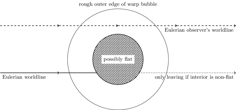
Figure 1: Illustration of the key step for the proof of the violation of the NEC, viewed from the perspective of the bubble’s center. Eulerian observers as depicted here will be present in any warp drive. They will see a trace of the extrinsic curvature $K$ that is in violation of its monotonicity as predicted by the NEC. Eulerian observers entering a flat inner region will remain there as long as the bubble persists.

8 Discussion and conclusions

We have now demonstrated that all members of the general class of warp drives defined by Natário [10] violate the NEC. This significantly extends previously known results. This argument applies, in particular, to all three of the Alcubierre [9], Natário zero-expansion [10], and Lentz/Fell–Heisenberg zero-vorticity [1, 3] warp drives, and also (for slightly different reasons) to the model warp drives considered by Bobrick–Martire [2]. Because the NEC is violated then so are the WEC, SEC, and DEC.

Consequently, insofar as one wishes to continue to entertain the possibility of warp drives as a real physical phenomenon, one has no choice but to face the violation of the energy conditions head on. Several possibilities arise: (i) modify the theory of gravity, (ii) modify the definition of warp drive, (iii) modify the energy conditions, (iv) appeal to macroscopic quantum physics, (v) allow for singularities or CTCs (time travel). None of these options are particularly palatable. All of these options have serious draw-backs. Thus it is our melancholy duty to report that none of the recent claims of positive-mass physical warp drives survive careful inspection of the proffered arguments.

Appendix A “Spherically symmetric” warp drives

“Spherically symmetric” warp drives date back to the original article by Alcubierre [9]. Specifically, let us reconsider the explicit line element (2.12) and rephrase it as

$${\mathrm{d}}s^{2}=-{\mathrm{d}}t^{2}+{\mathrm{d}}x^{2}+{\mathrm{d}}y^{2}+\Big{(}{\mathrm{d}}z-v_{*}(t)\;f\left(r_{s}(x,y,z,t)\right){\mathrm{d}}t\Big{)}^{2},$$ (A.1)

where we set

$$r_{s}(x,y,z,t)=\sqrt{x^{2}+y^{2}+\left(z-z_{*}(t)\right)^{2}}\,,\qquad z_{*}(t)=\int v_{*}(t)\,{\mathrm{d}}t,$$ (A.2)

and enforce both $f(0)=1$ and $f(\infty)=0$. This represents a spherically symmetric warp bubble, centred on the moving point $(0,0,z_{*}(t))$, with a shape function $f(r_{s})$ that depends only on the Euclidean distance from the moving centre. We emphasize that while the warp bubble is spherically symmetric the spacetime is not — there is certainly a preferred axis due to the direction of motion of the warp bubble. (Hence the warp bubble is spherically symmetric, but the spacetime is only “spherically symmetric”.) At large spatial distances ${\mathrm{d}}s^{2}\to-{\mathrm{d}}t^{2}+{\mathrm{d}}x^{2}+{\mathrm{d}}y^{2}+{\mathrm{d}}z^{2}$, the usual representation of Minkowski space, while at the centre of the warp drive

$${\mathrm{d}}s^{2}\to-{\mathrm{d}}t^{2}+{\mathrm{d}}x^{2}+{\mathrm{d}}y^{2}+\left({\mathrm{d}}z-v_{*}(t){\mathrm{d}}t\right)^{2}.$$ (A.3)

Consider now the coordinate transformation

$$\tilde{t}=t,\qquad\tilde{x}=x,\qquad\tilde{y}=y,\qquad\tilde{z}=z-z_{*}(t),$$ (A.4)

which is designed to bring the warp bubble “to rest”. Then

$${\mathrm{d}}\tilde{t}={\mathrm{d}}t,\qquad{\mathrm{d}}\tilde{x}={\mathrm{d}}x,\qquad{\mathrm{d}}\tilde{y}={\mathrm{d}}y,\qquad{\mathrm{d}}\tilde{z}={\mathrm{d}}z-v_{*}(t)\,{\mathrm{d}}t,$$ (A.5)

and the line element becomes

$${\mathrm{d}}s^{2}=-{\mathrm{d}}\tilde{t}^{2}+{\mathrm{d}}\tilde{x}^{2}+{\mathrm{d}}\tilde{y}^{2}+\left({\mathrm{d}}\tilde{z}+v_{*}(t)[1-f(r_{s})]\,{\mathrm{d}}\tilde{t}\right)^{2},$$ (A.6)

where now $r_{s}=\sqrt{\tilde{x}^{2}+\tilde{y}^{2}+\tilde{z}^{2}}$ is time independent. At the centre of the warp bubble we now have ${\mathrm{d}}s^{2}\to-{\mathrm{d}}\tilde{t}^{2}+{\mathrm{d}}\tilde{x}^{2}+{\mathrm{d}}\tilde{y}^{2}+{\mathrm{d}}\tilde{z}^{2}$, the usual representation of Minkowski space, while at spatial infinity it is now the outside universe that is streaming by with velocity $-v_{*}(t)$.

At spatial infinity the line element becomes

$${\mathrm{d}}s^{2}\to-{\mathrm{d}}\tilde{t}^{2}+{\mathrm{d}}\tilde{x}^{2}+{\mathrm{d}}\tilde{y}^{2}+\left({\mathrm{d}}\tilde{z}+v_{*}(t)\,{\mathrm{d}}\tilde{t}\right)^{2}.$$ (A.7)

This is again Minkowski space, but now in “moving coordinates”. Note the “conservation” of relative motion — either spatial infinity is standing still and the bubble is moving, or the bubble is standing still and spatial infinity is moving [9, 10].

If one wishes to make the walls of the warp bubble thin, (but still of finite thickness), this is a choice, not a necessity, then one might pick

$$f(r_{s})=\left\{\begin{array}[]{ll}1&\quad r_{s}\leq r_{\text{inner}},\\ \hbox{smooth}&\quad r_{s}\in[r_{\text{inner}},r_{\text{outer}}],\\ 0&\quad r_{s}\geq r_{\text{outer}}.\\ \end{array}\right.$$ (A.8)

If one makes this choice, then one needs to enforce $r_{\text{outer}}>r_{\text{inner}}$ to keep the metric continuous. A discontinuity in the metric leads to delta functions in the Christoffel symbols, squares of delta functions in the Riemann tensor, and cubes of delta functions in the Bianchi identities. Even when working with the Israel–Lanczos–Sen thin-shell formalism (the junction condition formalism) one needs to keep the metric piecewise differentiable, $C^{1-}$, since then the Christoffel symbols at worst contain step functions and the Riemann tensor and Bianchi identities at worst contain delta functions.

The reason for being so explicit is that in reference [2] the authors present a deeply flawed discussion of spherically symmetric warp drives. In their implementation of spherically symmetric warp drives the warp bubble is certainly at rest, but in addition their choice of asymptotic boundary conditions also forces the warp bubble to be at rest with respect to spatial infinity. This defeats the whole purpose of a warp drive.

Furthermore, these authors take the interior of the warp bubble to be a portion of flat Minkowski space, the wall of the warp bubble to be a non-negative density barotropic and isotropic fluid, and the exterior region to be a portion of Schwarzschild spacetime. They then attempt to apply the Tolman–Oppenheimer–Volkov (TOV) equation to the bubble wall. But under the set of assumptions they are imposing (zero pressure at the inner edge of the bubble wall, zero pressure at the outer edge of the bubble wall, non-negative energy density within the bubble wall, and a barotropic equation of state) the unique solution to the TOV is the trivial solution $p(r)=0=\rho(r)$, and the mass of the exterior region must be zero. Thus their specific model (as presented in [2]) just reduces, globally, to flat Minkowski space — it is not a warp drive.

These authors [2] also assert that both Alcubierre [9] and Natário [10] must necessarily “truncate” their warp fields, forcing them to be exactly Minkowski space, at some finite distance from the centre of the warp bubble. This is simply not an accurate reflection of what is actually done in those references [9, 10]. Specifically, in Alcubierre’s original article [9, equation (6)] the concrete realization of the shape function $f(r_{s})$ he chooses, see equation (A.8), uses tanh functions and so does not have compact support. In this terminology, Alcubierre sets $r_{\text{inner}}=0$ and $r_{\text{outer}}=\infty$, which is certainly not a truncation. Unfortunately this terminology of “truncation” has been uncritically adopted by subsequent authors [3].

The authors of [2] also assert in passing, see their section (5.2), that the Alcubierre warp drive [9] does not satisfy the continuity equations. They also assert that the velocity of the Alcubierre warp bubble cannot be time dependent, claiming a violation of the conservation of momentum. These statements are both false, and seem to arise (at best) from adopting a naive Newtonian viewpoint. What Alcubierre has actually done is to “reverse engineer” the warp drive — once one writes down a suitable metric, (at least $C^{1-}$, piecewise differentiable), one simply calculates the Einstein tensor to find what the stress-energy is that would be required to support that spacetime geometry. The continuity equation is automatically enforced via the Bianchi identities, and there is no difficulty in making the velocity of the Alcubierre warp bubble time-dependent. (Reference [3] seems to repeat this error in their discussion. Reference [1] is more careful in this regard, setting the 3-velocity of their model warp bubble constant for simplicity, but without making any claim as to necessity.)

Overall, while the idea of a “spherically symmetric” warp drive is certainly well-defined and useful, the specific implementation of this notion in reference [2] is not a successful one, and is not useful.

Appendix B Warp drives beyond the generic Natário framework

There are two somewhat more general warp drive spacetimes that do not fall into Natário’s general classification [10], and are incompatible with the Alcubierre, Natário, and Lentz/Fell–Heisenberg warp drives. These more general warp drives are obtained by either relaxing the condition that the lapse be unity, (so $N(x,y,z,t)\neq 1$), or relaxing the condition that the spatial slices be flat, (so $g_{ij}\neq\delta_{ij}$). See reference [29] which discusses the case $N\neq 1$, and reference [17] which permits the spatial slices to be conformally flat $g_{ij}=e^{2\theta(x,y,z,t)}\;\delta_{ij}$ rather than Riemann flat.

Unhelpfully, in appendices A.1 and A.2 of reference [2] those authors incorrectly claim that both of these more general spacetimes can, by a coordinate transformation, be brought into Alcubierre form. The simplest way to see that both these claims are wrong is to set the flow vector to zero. The claims made in appendices A.1 and A.2 of reference [2] then reduce to the claims that the line elements

$${\mathrm{d}}s^{2}=-N(x,y,z,t)^{2}{\mathrm{d}}t^{2}+{\mathrm{d}}x^{2}+{\mathrm{d}}y^{2}+{\mathrm{d}}z^{2},$$ (B.1)

and

$${\mathrm{d}}s^{2}=-{\mathrm{d}}t^{2}+e^{2\theta(x,y,z,t)}\{{\mathrm{d}}x^{2}+{\mathrm{d}}y^{2}+{\mathrm{d}}z^{2}\},$$ (B.2)

are actually Riemann flat. This is manifestly incorrect. What has gone wrong? The transformations these authors invoke are just not coordinate transformations. For a transformation ${\mathrm{d}}x^{a}\to{\mathrm{d}}\bar{x}^{a}=J^{a}{}_{b}\;{\mathrm{d}}x^{b}$ to actually be a coordinate transformation the critical requirement is that $J^{a}{}_{[b,c]}=0$. (Additionally, one would want $\det(J^{a}{}_{b})\neq 0$, except on sets of measure zero.) While the transformations made in appendices A.1 and A.2 of reference [2] satisfy the determinant condition, they fail the more basic $J^{a}{}_{[b,c]}=0$ condition; they are simply not coordinate transformations.

For our purposes then it means that the non-unit-lapse and van den Broeck warp drive spacetimes cannot simply be dismissed out of hand. There are other problematic issues with both of these models, but they are physically different from the Natário class [10], (unit lapse, spatially flat 3-geometry), and must be directly addressed using different techniques.

Appendix C Some defective warp drives

Some of the recently proposed warp drive spacetimes are defective for other reasons.

For instance, in the first explicit example in reference [3] the velocity potential $\Phi$ is certainly $C^{0}$ but is only piecewise differentiable, $C^{1-}$. That is, the flow $\vec{v}=\gradient\Phi$ is discontinuous, which implies that the metric is discontinuous. This then leads to delta functions in the Christoffel symbols, squares of delta functions in the Riemann tensor, and cubes of delta functions in the Bianchi identities. This is mathematically and physically not viable.

In their second explicit example, equation (9) of versions 1 and 2; equation (11) of versions 3 and 4 of reference [3], the velocity potential $\Phi$ is $C^{\infty}$, except possibly at the centre of the spacetime, but suffers other problems. If one takes $r=\sqrt{x^{2}+y^{2}+z^{2}}$, then even at its most general their velocity potential is of the qualitative form

$$\Phi(x,y,z)=F(r,\sigma(x,y,z))+v_{*}\,z.$$ (C.1)

Then

$$\vec{v}=\gradient\Phi(x,y,z)=\partial_{r}F(r,\sigma(x,y,z))\,\hat{r}+\partial_{\sigma}F(r,\sigma(x,y,z))\,\gradient\sigma+v_{*}\,\hat{z}.$$ (C.2)

But then, in their specific example, they do the equivalent of settting $\sigma(x,y,z)\to 1$, and $v_{*}\to 0$, thereby enforcing spherical symmetry. That is $\Phi(x,y,z)\to F(r,1)$, which is a function of $r$ only. But then

$$\vec{v}=\gradient\Phi\to{\partial F(r,1)\over\partial r}\;\;\hat{r}.$$ (C.3)

So their flow vector is always pointing radially outwards/inwards. This is simply not viable for describing a warp drive spacetime.

Oddly enough, consider $\Phi(x,y,z)=2\sqrt{2mr}=2\sqrt{2m}\;\sqrt[4]{x^{2}+y^{2}+z^{2}}$, so that

$$\vec{v}=\gradient\Phi(x,y,z)={\sqrt{2m}\;(x,y,z)\over(x^{2}+y^{2}+z^{2})^{3/4}}=\sqrt{2m\over\sqrt{x^{2}+y^{2}+z^{2}}}\;\;\hat{r}.$$ (C.4)

This is the Schwarzschild spacetime (in Painlevé–Gullstrand form, converted to Cartesian coordinates). This is not a warp drive spacetime.

Similarly, consider $\Phi(x,y,z)={(x^{2}+y^{2}+z^{2})\over 2\ell}$ so that

$$\vec{v}=\gradient\Phi={(x,y,z)\over\ell}={\sqrt{x^{2}+y^{2}+z^{2}}\over\ell}\;\hat{r}.$$ (C.5)

This is the de Sitter spacetime (in Painlevé–Gullstrand form, converted to Cartesian coordinates, with $\Lambda=3/\ell^{2}$). This is not a warp drive spacetime.

But the central issue is this: Even if you pick a flow vector of the form

$$\vec{v}=f(r)\;\hat{r}+v_{*}\;\hat{z},$$ (C.6)

which at least has a hope of representing a moving warp bubble, then calculating and checking the non-negativity of the Eulerian energy density $\rho$ by itself tells you next to nothing regarding satisfaction of the WEC. To test satisfaction of the WEC one would need to calculate all of the principal pressures $p_{i}$ and then check whether all of the combinations $\rho+p_{i}$ were non-negative.

In reference [1] the claim is made that the author can self-consistently find a warp drive configuration that is sourced by a perfect fluid plasma (satisfying the WEC and so also the NEC) plus electromagnetic Maxwell stress-energy (satisfying all of NEC, WEC, SEC, and DEC). So if this claim were to be true, if these models truly were solutions of the Einstein equations with the specified source, one would have a warp drive spacetime satisfying the NEC, which we have just shown to be impossible. What has gone wrong? The point here is that the author of [1] has not actually solved the Einstein equations, he has only solved part of the Einstein equations — for the density, flux, and trace of the stress. This is not enough to obtain a valid solution of the Einstein equations — the author would also need to consider the remaining trace-free part $T_{ij}-{1\over 3}(T_{kl}\delta^{kl})g_{ij}$ of the stress tensor.

Appendix D Final considerations regarding recent warp drive proposals

We would like to conclude by explicitly explaining (if not yet mentioned) why each of the recent warp drive proposals have failed in their claims.

Starting with [1], the author has claimed to have found a warp drive solution which would not violate the WEC. This is actually an incorrect claim since the author has never actually solved the Einstein equations. By imposing a warp drive metric, it is clear from equations (3.19), (3.20) and (3.21) that all of the components of the energy momentum tensor are already determined, without much freedom to play around. This is called a reverse engineering process. Once you define your metric, your energy momentum tensor follows directly from it. The author, however, imposes not only the metric, but also an energy momentum tensor — therefore imposing both sides of the Einstein equations without ever verifying if they are indeed an equation or not. Hence, they haven’t only not found a solution which satisfies the WEC, they haven’t found a solution at all.

Proceeding with [2], their warp drives are divided into two classes: “General spherically symmetric warp drives”, which we already discussed in appendix A, and “Axisymmetric warp drives with a general internal region” in which they haven’t found any metric satisfying the WEC. In this way, their only “warp drive” which satisfies the WEC is actually not a warp drive metric at all. It is a static spherically symmetric spacetime, therefore being reduced to either Minkowski or Schwarzschild. Furthermore, their claims about Alcubierre’s warp drive requiring negative energy due to the “artificial” matching rate for the clocks inside and outside the warp drive follows directly from their rediscovery of the existence of time delays in Schwarzschild spacetimes, which they believe to be a warp drive.

Finally, in [3], their main issue reduces to “proving” the WEC by calculating the energy density for a unique class of observers – the Eulerian observers. As mentioned already, to prove the WEC one needs to prove that the energy density is positive for all time-like observers and, proving only for one class of observers simply doesn’t prove anything. Furthermore, the specific examples provided by them have a great deal of problems, as already explained in appendix C.

The series of articles by Santos-Pereira, Abreu, and Ribeiro [4, 5, 6, 7, 8], has other issues. Specifically:

• Their perfect fluid warp drives (dust, non-zero pressure, non-zero pressure with cosmological constant) are just Riemann-flat Minkowski space in disguise.

• Their anisotropic fluid warp drive (“parameterized perfect fluid” warp drive) is less trivial, but is still seriously diseased.

• Their charged dust warp drive is less trivial, but is still seriously diseased.
  (Among other things, the calculation of energy density is deeply flawed, confusing $T_{00}$ and $T^{00}$.)

• Their “cosmological” warp drive is not cosmological.

We shall go into some detail in an attempt to make the situation clear and transparent.

The earliest paper [4] analyzes the Alcubierre warp drive with a stress-energy that is pure comoving Eulerian dust. Now this is a very strong constraint, and one quickly deduces that the energy density of the dust is zero. This means that the entire stress-energy tensor is identically zero; so one is looking for vacuum solutions of the Einstein equations for an Alcubierre warp drive. But the set of vacuum solutions in an Alcubierre warp drive framework is extremely limited — in fact once one completely satisfies all the Einstein equations the only such solution is Riemann-flat Minkowski space (which, viewed as a warp drive, is trivial).

The anisotropic fluid (“parameterized perfect fluid”) studied in [5] has the defect that once one completely satisfies all the Einstein equations the “warp drive” is infinitely wide in the transverse directions — so it is not a warp “bubble”, the warp field stretches all the way across the universe in the $y$ and $z$ directions; one is trying to accelerate an entire “slab” of spacetime in the $x$ direction. Furthermore, the Eulerian energy density, flux, and pressure in the direction of motion are zero, the pressures transverse to the direction of motion are equal and possibly nonzero — this would then certainly violate the DEC.

For the charged dust solution of [6] there is a technical error in identifying the energy density. The physically interesting quantity is $\rho=T^{00}=T^{ab}\;(-1;0,0,0)_{a}\;(-1;0,0,0)_{b}$, where the 4-covector $(-1;0,0,0)_{a}$ is always timelike and future pointing (it is in fact the 4-velocity of an Eulerian observer). In contrast the quantity $T_{00}=T_{ab}\;(1;0,0,0)^{a}\;(1;0,0,0)^{b}$ is not physically interesting since the 4-vector $(1;0,0,0)^{a}$ is timelike only for a limited range of warp velocities; in fact, this 4-vector becomes spacelike exactly when the warp bubble motion becomes superluminal.

For the “cosmological” solution of [7] the attempt at including a cosmological constant is at best a redefinition of terms in the stress-energy tensor. For instance, the definition of Einstein tensor adopted in [7] is not the usual one, which is unhelpful. Furthermore, given that the entire calculation is taking place within the framework of the generic Alcubierre metric, we know the spacetime is asymptotically flat; it does not match (anti)de Sitter at large distances, so it is not a “cosmological” warp bubble.

In all of these situations [4, 5, 6, 7, 8], one is working within the framework of the generic Alcubierre metric, so we know from first principles that energy condition violations must be present.

References

- [1] E. W. Lentz, “Breaking the warp barrier: hyper-fast solitons in Einstein–Maxwell-plasma theory”, Class. Quant. Grav. 38 (2021) no.7, 075015 doi:10.1088/1361-6382/abe692 [arXiv:2006.07125 [gr-qc]].
-
[2]
A. Bobrick and G. Martire,
“Introducing physical warp drives”,
Class. Quant. Grav. 38 (2021) no.10, 105009 doi:10.1088/1361-6382/abdf6e [arXiv:2102.06824 [gr-qc]]. - [3] S. D. B. Fell and L. Heisenberg, “Positive energy warp drive from hidden geometric structures”, Class.Quant.Grav. 38 (2021) 155020 doi:10.1088/1361-6382/ac0e47 [arXiv:2104.06488 [gr-qc]].
- [4] O. L. Santos-Pereira, E. M. C. Abreu and M. B. Ribeiro, “Dust content solutions for the Alcubierre warp drive spacetime”, Eur. Phys. J. C 80 (2020) no.8, 786 doi:10.1140/epjc/s10052-020-8355-2 [arXiv:2008.06560 [gr-qc]].
- [5] O. L. Santos-Pereira, E. M. C. Abreu and M. B. Ribeiro, “Fluid dynamics in the warp drive spacetime geometry”, Eur. Phys. J. C 81 (2021) no.2, 133 doi:10.1140/epjc/s10052-021-08921-3 [arXiv:2101.11467 [gr-qc]].
- [6] O. L. Santos-Pereira, E. M. C. Abreu and M. B. Ribeiro, “Charged dust solutions for the warp drive spacetime”, Gen. Rel. Grav. 53 (2021) no.2, 23 doi:10.1007/s10714-021-02799-y [arXiv:2102.05119 [gr-qc]].
- [7] O. L. Santos-Pereira, E. M. C. Abreu and M. B. Ribeiro, “Perfect fluid warp drive solutions with the cosmological constant”, Eur. Phys. J. Plus 136 (2021) no.9, 902 doi:10.1140/epjp/s13360-021-01899-7 [arXiv:2108.10960 [gr-qc]].
- [8] O. L. Santos-Pereira, E. M. C. Abreu and M. B. Ribeiro, “Warp drive dynamic solutions considering different fluid sources”, MG16 Conference Proceedings, [arXiv:2111.01298 [gr-qc]].
-
[9]
M. Alcubierre,
“The Warp drive: Hyperfast travel within general relativity”,
Class. Quant. Grav. 11 (1994), L73-L77 doi:10.1088/0264-9381/11/5/001 [arXiv:gr-qc/0009013 [gr-qc]]. -
[10]
J. Natário,
“Warp drive with zero expansion”,
Class. Quant. Grav. 19 (2002), 1157-1166 doi:10.1088/0264-9381/19/6/308 [arXiv:gr-qc/0110086 [gr-qc]]. - [11] A. E. Everett, “Warp drive and causality”, Phys. Rev. D 53 (1996), 7365-7368 doi:10.1103/PhysRevD.53.7365
- [12] A. E. Everett and T. A. Roman, “A Superluminal subway: The Krasnikov tube”, Phys. Rev. D 56 (1997), 2100-2108 doi:10.1103/PhysRevD.56.2100 [arXiv:gr-qc/9702049 [gr-qc]].
-
[13]
W. A. Hiscock,
“Quantum effects in the Alcubierre warp drive space-time”,
Class. Quant. Grav. 14 (1997), L183-L188 doi:10.1088/0264-9381/14/11/002 [arXiv:gr-qc/9707024 [gr-qc]]. - [14] M. J. Pfenning, “Quantum inequality restrictions on negative energy densities in curved space-times”, [arXiv:gr-qc/9805037 [gr-qc]].
- [15] R. J. Low, “Speed limits in general relativity”, Class. Quant. Grav. 16 (1999), 543-549 doi:10.1088/0264-9381/16/2/016 [arXiv:gr-qc/9812067 [gr-qc]].
- [16] K. D. Olum, “Superluminal travel requires negative energies”, Phys. Rev. Lett. 81 (1998), 3567-3570 doi:10.1103/PhysRevLett.81.3567 [arXiv:gr-qc/9805003 [gr-qc]].
-
[17]
C. Van Den Broeck,
“A warp drive with reasonable total energy requirements”,
Class. Quant. Grav. 16 (1999), 3973-3979 doi:10.1088/0264-9381/16/12/314 [arXiv:gr-qc/9905084 [gr-qc]]. - [18] C. Van Den Broeck, “On the (im)possibility of warp bubbles”, [arXiv:gr-qc/9906050 [gr-qc]].
- [19] C. Clark, W. A. Hiscock and S. L. Larson, “Null geodesics in the Alcubierre warp drive space-time: The view from the bridge”, Class. Quant. Grav. 16 (1999), 3965-3972 doi:10.1088/0264-9381/16/12/313 [arXiv:gr-qc/9907019 [gr-qc]].
- [20] M. Visser, B. Bassett and S. Liberati, “Perturbative superluminal censorship and the null energy condition”, AIP Conf. Proc. 493 (1999) no.1, 301-305 doi:10.1063/1.1301601 [arXiv:gr-qc/9908023 [gr-qc]].
- [21] M. Alcubierre, “Warp-Antrieb — Wurmlöcher — Zeitreisen” (“Warp propulsion, wormholes, time travel”), Sterne und Weltraum special 6 (2001), 70-76
- [22] F. S. N. Lobo and P. Crawford, “Weak energy condition violation and superluminal travel”, Lect. Notes Phys. 617 (2003), 277-291 [arXiv:gr-qc/0204038 [gr-qc]].
- [23] F. S. N. Lobo and M. Visser, “Fundamental limitations on warp drive spacetimes”, Class. Quant. Grav. 21 (2004), 5871-5892 doi:10.1088/0264-9381/21/24/011 [arXiv:gr-qc/0406083 [gr-qc]].
- [24] F. S. N. Lobo and M. Visser, “Linearized warp drive and the energy conditions”, Proceedings of the Spanish Relativity Meeting-2004 (Miraflores de la Sierra, Madrid, September 2004) [arXiv:gr-qc/0412065 [gr-qc]].
-
[25]
F. S. N. Lobo,
“Exotic solutions in General Relativity: Traversable wormholes and warp drive spacetimes”,
Classical and Quantum Gravity Research (2008) 1–78,
Nova Sci. Pub. (New York), ISBN-10: 978-1-60456-366-5 [arXiv:0710.4474 [gr-qc]]. - [26] S. Finazzi, S. Liberati and C. Barceló, “Semiclassical instability of dynamical warp drives”, Phys. Rev. D 79 (2009), 124017 doi:10.1103/PhysRevD.79.124017 [arXiv:0904.0141 [gr-qc]].
- [27] B. McMonigal, G. F. Lewis and P. O’Byrne, “The Alcubierre warp drive: On the matter of matter”, Phys. Rev. D 85 (2012), 064024 doi:10.1103/PhysRevD.85.064024 [arXiv:1202.5708 [gr-qc]].
- [28] M. Alcubierre and F. S. N. Lobo, “Wormholes, Warp Drives and Energy Conditions”, Fundam. Theor. Phys. 189 (2017), pp.1-279 doi:10.1007/978-3-319-55182-1 [arXiv:2103.05610 [gr-qc]].
-
[29]
M. Alcubierre and F. S. N. Lobo,
“Warp Drive Basics”,
Fundam. Theor. Phys. 189 (2017), 257-279 doi:10.1007/978-3-319-55182-1_11 [arXiv:2103.05610 [gr-qc]] -
[30]
R. L. Arnowitt, S. Deser and C. W. Misner,
“The Dynamics of general relativity”,
Originally published in “Gravitation: an introduction to current research”,
edited by Louis Witten (Wiley 1962), chapter 7, pp 227–265.
Republished as: Gen. Rel. Grav. 40 (2008), 1997-2027 doi:10.1007/s10714-008-0661-1 [arXiv:gr-qc/0405109 [gr-qc]]. -
[31]
E. Gourgoulhon,
“3+1 formalism and bases of numerical relativity”,
Lecture Notes in Physics 846, (Springer-Verlag, Berlin, 2012)
ISBN-13: 978-3-642-24524-4 [arXiv:gr-qc/0703035 [gr-qc]]. - [32] R. M. Wald, General Relativity, (University of Chicago Press, Chicago, 1984) ISBN-10: 0-226-87033-2 doi:10.7208/chicago/9780226870373.001.0001
- [33] E. Poisson, A Relativist’s Toolkit: The Mathematics of Black-Hole Mechanics, (Cambridge, Cambridge, 2004) ISBN-10: 0-521-83091-5 doi:10.1017/CBO9780511606601
- [34] C. W. Misner, K. S. Thorne and J. A. Wheeler, Gravitation, (Freeman, San Francisco, 1973) ISBN-10: 0-7167-0334-3
- [35] C. Kiefer, Quantum gravity, (Oxford University Press, Oxford, 2007) ISBN-13: 978-0-19-958520-5.
- [36] M. Alcubierre, Introduction to 3+1 Numerical Relativity, (Oxford, Oxford, 2008) ISBN-13: 9780199205677 doi:10.1093/acprof:oso/9780199205677.001.0001
- [37] W. G. Unruh, “Experimental black hole evaporation”, Phys. Rev. Lett. 46 (1981), 1351-1353 doi:10.1103/PhysRevLett.46.1351
- [38] C. Barceló, S. Liberati and M. Visser, “Analogue gravity”, Living Rev. Rel. 8 (2005), 12 doi:10.12942/lrr-2005-12 [arXiv:gr-qc/0505065 [gr-qc]].
- [39] M. Visser, “Acoustic black holes: Horizons, ergospheres, and Hawking radiation”, Class. Quant. Grav. 15 (1998), 1767-1791 doi:10.1088/0264-9381/15/6/024 [arXiv:gr-qc/9712010 [gr-qc]].
- [40] M. Novello, M. Visser and G. Volovik, Artificial black holes, (World Scientific, Singapore, 2002) ISBN-13: 978-981-02-4807-9
- [41] R. Schutzhold and W. G. Unruh, “Gravity wave analogs of black holes”, Phys. Rev. D 66 (2002), 044019 doi:10.1103/PhysRevD.66.044019 [arXiv:gr-qc/0205099 [gr-qc]].
- [42] S. W. Hawking and G. F. R. Ellis, The large scale structure of space-time, ISBN-13: 978-0-521-09906-6 doi:10.1017/CBO9780511524646
- [43] M. Visser, Lorentzian wormholes: From Einstein to Hawking, (AIP Press — now Springer, New York, 1995) ISBN-13: 978-1563966538 ISBN-10: 1563966530
- [44] E. Curiel, “A Primer on Energy Conditions”, Einstein Stud. 13 (2017), 43-104 doi:10.1007/978-1-4939-3210-8_3 [arXiv:1405.0403 [physics.hist-ph]].
- [45] E. A. Kontou and K. Sanders, “Energy conditions in general relativity and quantum field theory”, Class. Quant. Grav. 37 (2020) no.19, 193001 doi:10.1088/1361-6382/ab8fcf [arXiv:2003.01815 [gr-qc]].
- [46] S. M. Carroll, Spacetime and geometry: An introduction to general relativity, (Addison Wesley, San Francisco, 2004) ISBN-10: 0-8053-8732-3.
- [47] S. W. Hawking and W. Israel, editors, General relativity: An Einstein centenary survey, (Cambridge, Cambridge, 1979) ISBN-10: 0-521-29928-4.
- [48] H. Maeda and C. Martinez, “Energy conditions in arbitrary dimensions”, PTEP 2020 (2020) no.4, 043E02 doi:10.1093/ptep/ptaa009 [arXiv:1810.02487 [gr-qc]].
- [49] C. Barceló and M. Visser, “Twilight for the energy conditions?”, Int. J. Mod. Phys. D 11 (2002), 1553-1560 doi:10.1142/S0218271802002888 [arXiv:gr-qc/0205066 [gr-qc]].
-
[50]
J. D. Bekenstein,
“If vacuum energy can be negative, why is mass always positive?:
Uses of the subdominant trace energy condition”, Phys. Rev. D 88 (2013), 125005 doi:10.1103/PhysRevD.88.125005 [arXiv:1310.6203 [quant-ph]]. - [51] M. Visser and C. Barceló, “Energy conditions and their cosmological implications”, doi:10.1142/9789812792129_0014 [arXiv:gr-qc/0001099 [gr-qc]].
- [52] M. Visser, “General relativistic energy conditions: The Hubble expansion in the epoch of galaxy formation”, Phys. Rev. D 56 (1997), 7578-7587 doi:10.1103/PhysRevD.56.7578 [arXiv:gr-qc/9705070 [gr-qc]].
- [53] M. Visser, “Energy conditions in the epoch of galaxy formation”, Science 276 (1997), 88-90 doi:10.1126/science.276.5309.88 [arXiv:1501.01619 [gr-qc]].
- [54] M. Visser, “Energy conditions and galaxy formation”, [arXiv:gr-qc/9710010 [gr-qc]].
- [55] C. Cattoën and M. Visser, “Cosmodynamics: Energy conditions, Hubble bounds, density bounds, time and distance bounds”, Class. Quant. Grav. 25 (2008), 165013 doi:10.1088/0264-9381/25/16/165013 [arXiv:0712.1619 [gr-qc]].
-
[56]
C. Cattoën and M. Visser,
“Cosmological milestones and energy conditions”,
J. Phys. Conf. Ser. 68 (2007), 012011 doi:10.1088/1742-6596/68/1/012011 [arXiv:gr-qc/0609064 [gr-qc]]. -
[57]
E. A. Kontou and K. D. Olum,
“Energy conditions allow eternal inflation”,
JCAP 03 (2021), 097 doi:10.1088/1475-7516/2021/03/097 [arXiv:2008.01878 [gr-qc]]. -
[58]
A. Zee, Einstein gravity in a nutshell,
(Princeton, Princeton, 2013)
ISBN-13: 978-0-691-14558-7 - [59] P. Martín-Moruno and M. Visser, “Classical and quantum flux energy conditions for quantum vacuum states”, Phys. Rev. D 88 (2013) no.6, 061701 doi:10.1103/PhysRevD.88.061701 [arXiv:1305.1993 [gr-qc]].
- [60] P. Martín-Moruno and M. Visser, “Classical and semi-classical energy conditions”, Fundam. Theor. Phys. 189 (2017), 193-213 doi:10.1007/978-3-319-55182-1_9 [arXiv:1702.05915 [gr-qc]].
- [61] P. Martín-Moruno and M. Visser, “Semiclassical energy conditions for quantum vacuum states”, JHEP 09 (2013), 050 doi:10.1007/JHEP09(2013)050 [arXiv:1306.2076 [gr-qc]].
- [62] P. Martín-Moruno and M. Visser, “Semi-classical and nonlinear energy conditions”, doi:10.1142/9789813226609_0126 [arXiv:1510.00158 [gr-qc]].
- [63] M. Visser, “Gravitational vacuum polarization. 1: Energy conditions in the Hartle-Hawking vacuum”, Phys. Rev. D 54 (1996), 5103-5115 doi:10.1103/PhysRevD.54.5103 [arXiv:gr-qc/9604007 [gr-qc]].
- [64] M. Visser, “Gravitational vacuum polarization. 2: Energy conditions in the Boulware vacuum”, Phys. Rev. D 54 (1996), 5116-5122 doi:10.1103/PhysRevD.54.5116 [arXiv:gr-qc/9604008 [gr-qc]].
- [65] M. Visser, “Gravitational vacuum polarization. 3: Energy conditions in the (1+1) Schwarzschild space-time”, Phys. Rev. D 54 (1996), 5123-5128 doi:10.1103/PhysRevD.54.5123 [arXiv:gr-qc/9604009 [gr-qc]].
- [66] M. Visser, “Gravitational vacuum polarization. 4: Energy conditions in the Unruh vacuum”, Phys. Rev. D 56 (1997), 936-952 doi:10.1103/PhysRevD.56.936 [arXiv:gr-qc/9703001 [gr-qc]].
- [67] M. Visser, “Gravitational vacuum polarization”, Proceedings of MG8, the Eighth Marcel Grossmann Conference on General Relativity. (Jerusalem, Israel, June 1997) World Scientific (Singapore) ISBN-10: 981-02-3954-8 [arXiv:gr-qc/9710034 [gr-qc]].
- [68] C. J. Fewster and T. A. Roman, “Null energy conditions in quantum field theory”, Phys. Rev. D 67 (2003), 044003 [erratum: Phys. Rev. D 80 (2009), 069903] doi:10.1103/PhysRevD.67.044003 [arXiv:gr-qc/0209036 [gr-qc]].
- [69] C. J. Fewster and G. J. Galloway, “Singularity theorems from weakened energy conditions”, Class. Quant. Grav. 28 (2011), 125009 doi:10.1088/0264-9381/28/12/125009 [arXiv:1012.6038 [gr-qc]].
- [70] C. J. Fewster, “Lectures on quantum energy inequalities”, [arXiv:1208.5399 [gr-qc]].
- [71] M. Visser, “Scale anomalies imply violation of the averaged null energy condition”, Phys. Lett. B 349 (1995), 443-447 doi:10.1016/0370-2693(95)00303-3 [arXiv:gr-qc/9409043 [gr-qc]].
- [72] E. E. Flanagan and R. M. Wald, “Does back reaction enforce the averaged null energy condition in semiclassical gravity?”, Phys. Rev. D 54 (1996), 6233-6283 doi:10.1103/PhysRevD.54.6233 [arXiv:gr-qc/9602052 [gr-qc]].
- [73] L. H. Ford and T. A. Roman, “Averaged energy conditions and quantum inequalities”, Phys. Rev. D 51 (1995), 4277-4286 doi:10.1103/PhysRevD.51.4277 [arXiv:gr-qc/9410043 [gr-qc]].
- [74] L. H. Ford and T. A. Roman, “Averaged energy conditions and evaporating black holes”, Phys. Rev. D 53 (1996), 1988-2000 doi:10.1103/PhysRevD.53.1988 [arXiv:gr-qc/9506052 [gr-qc]].
- [75] L. H. Ford, “The Classical singularity theorems and their quantum loop holes”, Int. J. Theor. Phys. 42 (2003), 1219-1227 doi:10.1023/A:1025754515197 [arXiv:gr-qc/0301045 [gr-qc]].
- [76] L. H. Ford, “Spacetime in semiclassical gravity”, doi:10.1142/9789812700988_0011 [arXiv:gr-qc/0504096 [gr-qc]].
- [77] R. M. Wald and U. Yurtsever, “General proof of the averaged null energy condition for a massless scalar field in two-dimensional curved space-time”, Phys. Rev. D 44 (1991), 403-416 doi:10.1103/PhysRevD.44.403
- [78] M. Visser, S. Kar and N. Dadhich, “Traversable wormholes with arbitrarily small energy condition violations”, Phys. Rev. Lett. 90 (2003), 201102 doi:10.1103/PhysRevLett.90.201102 [arXiv:gr-qc/0301003 [gr-qc]].
- [79] D. Hochberg and M. Visser, “Dynamic wormholes, anti-trapped surfaces, and energy conditions”, Phys. Rev. D 58 (1998), 044021 doi:10.1103/PhysRevD.58.044021 [arXiv:gr-qc/9802046 [gr-qc]].
- [80] D. Hochberg and M. Visser, “The Null energy condition in dynamic wormholes”, Phys. Rev. Lett. 81 (1998), 746-749 doi:10.1103/PhysRevLett.81.746 [arXiv:gr-qc/9802048 [gr-qc]].
- [81] C. Barceló and M. Visser, “Scalar fields, energy conditions, and traversable wormholes”, Class. Quant. Grav. 17 (2000), 3843-3864 doi:10.1088/0264-9381/17/18/318 [arXiv:gr-qc/0003025 [gr-qc]].
- [82] C. Barceló and M. Visser, “Brane surgery: Energy conditions, traversable wormholes, and voids”, Nucl. Phys. B 584 (2000), 415-435 doi:10.1016/S0550-3213(00)00379-5 [arXiv:hep-th/0004022 [hep-th]].
- [83] S. Kar, N. Dadhich and M. Visser, “Quantifying energy condition violations in traversable wormholes”, Pramana 63 (2004), 859-864 doi:10.1007/BF02705207 [arXiv:gr-qc/0405103 [gr-qc]].
- [84] T. A. Roman and P. G. Bergmann, “Stellar collapse without singularities?”, Phys. Rev. D 28 (1983), 1265-1277 doi:10.1103/PhysRevD.28.1265
- [85] T. A. Roman, “Some thoughts on energy conditions and wormholes”, doi:10.1142/9789812704030_0236 [arXiv:gr-qc/0409090 [gr-qc]].
- [86] F. S. N. Lobo, “From the Flamm–Einstein–Rosen bridge to the modern renaissance of traversable wormholes”, Int. J. Mod. Phys. D 25 (2016) no.07, 1630017 doi:10.1142/S0218271816300172 [arXiv:1604.02082 [gr-qc]].
- [87] D. Hochberg, C. Molina-París and M. Visser, “Tolman wormholes violate the strong energy condition”, Phys. Rev. D 59 (1999), 044011 doi:10.1103/PhysRevD.59.044011 [arXiv:gr-qc/9810029 [gr-qc]].
- [88] S. W. Hawking, “Chronology protection conjecture”, Phys. Rev. D. 46 (2) (1992) 603. doi:10.1103/physrevd.46.603.
- [89] M. Visser, “The Quantum physics of chronology protection”, Published in: The Future of Theoretical Physics and Cosmology, Celebrating Steven Hawking’s 60th Birthday, Edited by G. W. Gibbons, E. P. S. Shellard, and S. J. Drake, (Cambridge, Cambridge, 2003) ISBN-13: 978-0-521-14408-7 [arXiv:gr-qc/0204022 [gr-qc]].
- [90] M. Visser, “From wormhole to time machine: Comments on Hawking’s chronology protection conjecture”, Phys. Rev. D 47 (1993), 554-565 doi:10.1103/PhysRevD.47.554 [arXiv:hep-th/9202090 [hep-th]].
- [91] M. Visser, “Hawking’s chronology protection conjecture: Singularity structure of the quantum stress-energy tensor”, Nucl. Phys. B 416 (1994), 895-906 doi:10.1016/0550-3213(94)90560-6 [arXiv:hep-th/9303023 [hep-th]].
- [92] J. L. Friedman and A. Higuchi, “Topological censorship and chronology protection”, Annalen Phys. 15 (2006), 109-128 doi:10.1002/andp.200510172 [arXiv:0801.0735 [gr-qc]].
- [93] S. Liberati, “Do not mess with time: Probing faster than light travel and chronology protection with superluminal warp drives”, doi:10.1142/9789813226609_0120 [arXiv:1601.00785 [gr-qc]].
- [94] M. J. Pfenning and L. H. Ford, “The unphysical nature of “Warp Drive””, Class. Quant. Grav. 14 (1997) no.7, 1743 doi:10.1088/0264-9381/14/7/011 [arXiv:gr-qc/9702026v3].
- [95] R. Gattermann, “Nadsvětelný pohyb v obecné relativitě”, (“Superluminal motion in general relativity”), Bachelor Thesis (2013), Charles University Prague doi:20.500.11956/55966
- [96] P. Martín-Moruno and M. Visser, “Essential core of the Hawking–Ellis types”, Class. Quant. Grav. 35 (2018) no.12, 125003 doi:10.1088/1361-6382/aac147 [arXiv:1802.00865 [gr-qc]].
- [97] P. Martín-Moruno and M. Visser, “Generalized Rainich conditions, generalized stress-energy conditions, and the Hawking-Ellis classification”, Class. Quant. Grav. 34 (2017) no.22, 225014 doi:10.1088/1361-6382/aa9039 [arXiv:1707.04172 [gr-qc]].
- [98] P. Martín-Moruno and M. Visser, “Hawking–Ellis type III spacetime geometry”, Class. Quant. Grav. 35 (2018) no.18, 185004 doi:10.1088/1361-6382/aad473 [arXiv:1806.02094 [gr-qc]].
- [99] P. Martín-Moruno and M. Visser, “The type III stress-energy tensor: Ugly duckling of the Hawking–Ellis classification”, Class. Quant. Grav. 37 (2020) no.1, 015013 doi:10.1088/1361-6382/ab56f6 [arXiv:1907.01269 [gr-qc]].
- [100] P. Martín-Moruno and M. Visser, “Hawking-Ellis classification of stress-energy: test-fields versus back-reaction”, [arXiv:2102.13551 [gr-qc]].
- [101] A. K. Raychaudhuri, “Relativistic cosmology I”, Phys. Rev. 98 #4 (1955) 1123?1126. doi:10.1103/PhysRev.98.1123.
- [102] S. Kar and S. SenGupta, “The Raychaudhuri equations: A Brief review”, Pramana 69 (2007), 49 doi:10.1007/s12043-007-0110-9 [arXiv:gr-qc/0611123 [gr-qc]].
- [103] N. Dadhich, “Derivation of the Raychaudhuri equation”, [arXiv:gr-qc/0511123 [gr-qc]].
- [104] J. Ehlers, “A. K. Raychaudhuri and his equation”, Int. J. Mod. Phys. D 15 (2006), 1573-1580 doi:10.1142/S0218271806008966
- [105] A. Borde, “Geodesic focusing, energy conditions and singularities”, Class. Quant. Grav. 4 (1987), 343-356 doi:10.1088/0264-9381/4/2/015
- [106] M. Visser, “van Vleck determinants: Geodesic focusing and defocusing in Lorentzian space-times”, Phys. Rev. D 47 (1993), 2395-2402 doi:10.1103/PhysRevD.47.2395 [arXiv:hep-th/9303020 [hep-th]].
- [107] G. Abreu and M. Visser, “Some generalizations of the Raychaudhuri equation”, Phys. Rev. D 83 (2011), 104016 doi:10.1103/PhysRevD.83.104016 [arXiv:1012.4806 [gr-qc]].