Broadband Spectral and Timing Properties of MAXI J1348–630 using AstroSat and NICER Observations

Abstract

We present broadband X-ray spectral-timing analysis of the new Galactic X-ray transient MAXI J1348–630 using five simultaneous AstroSat and NICER observations. Spectral analysis using AstroSat data identify the source to be in the soft state for the first three observations and in a faint and bright hard state for the next two. Quasi-periodic oscillations at $\sim 0.9$ and $\sim 6.9$ Hz, belonging to the type-C and type-A class are detected. In the soft state, the power density spectra are substantially lower (by a factor $>5$) for the NICER (0.5–12 keV) band compared to the AstroSat/LAXPC (3–80 keV) one, confirming that the disk is significantly less variable than the Comptonization component. For the first time, energy-dependent fractional rms and time lag in the 0.5–80 keV energy band was measured at different Fourier frequencies, using the bright hard state observation. Hard time lag is detected for the bright hard state, while the faint one shows evidence for soft lag. A single-zone propagation model fits the LAXPC results in the energy band 3–80 keV with parameters similar to those obtained for Cygnus X–1 and MAXI J1820+070. Extending the model to lower energies, reveals qualitative similarities but having quantitative differences with the NICER results. These discrepancies could be because the NICER and AstroSat data are not strictly simultaneous and because the simple propagation model does not take into account disk emission. The results highlight the need for more joint coordinated observations of such systems by NICER and AstroSat.

1 Introduction

Black hole transients (BHTs) are usually discovered when they exhibit outbursts, which are characterized by distinct spectral and temporal states (see Remillard & McClintock, 2006; Belloni et al., 2011, for reviews). Based on the spectro-timing properties, four main states have been identified in BHTs: the hard state (HS), the soft state (SS), the hard and soft intermediate states (HIMS and SIMS). In the HS, the source is characterized by a hard spectrum with a typical photon index $\Gamma\sim 1.7$. The power density spectra (PDS) are dominated by strong broad-limited noise with typical root mean square (rms) values of $\sim 30\%$ (Belloni, 2005) and occasionally exhibits type-C low-frequency quasi-periodic oscillations (LFQPOs) along with a sub-harmonic or second harmonic in the PDS. Type-C QPOs are characterized by a narrow peak with centroid frequency ranging from few mHz to $\sim 30$ Hz (Remillard et al., 2002; Casella et al., 2005). The SS spectra are dominated by a thermal disk component and the variability amplitude reduces to a few percent. Weak QPOs with a frequency range of 6–8 Hz are sometimes detected in the SS, which belong to the so-called type-A category (Wijnands et al., 1999; Casella et al., 2004; Motta et al., 2011; Motta, 2016). In the HIMS and SIMS, the energy spectrum is a combination of soft and hard components, while the PDS contains type-C LFQPOs in HIMS and type-A and B in the SIMS.

From 1996 to 2012, the Rossi X-ray Timing Explorer (RXTE) was the workhorse in the field of rapid time variability of X-ray binaries. Now the Large Area X-ray Proportional Counter (LAXPC) onboard AstroSat has replaced RXTE and is contributing to the rapid time variability studies in the hard energy band. For example, AstroSat data has been used to study the spectral-timing properties of several black hole X-ray binaries, including Cygnus X–1 (Misra et al., 2017; Maqbool et al., 2019), Cygnus X–3 (Pahari et al., 2017), MAXI J1535–571 (Bhargava et al., 2019; Sreehari et al., 2019), Swift J1658.2–4242 (Jithesh et al., 2019), GRS 1915+105 (Rawat et al., 2019; Belloni et al., 2019; Misra et al., 2020; Sreehari et al., 2020), MAXI J1820+070 (Mudambi et al., 2020) and 4U 1630–472 (Baby et al., 2020). The soft X-ray ($<4$ keV) rapid timing properties of black hole X-ray binaries (BHXRBs) were largely unknown, which is now being explored using the X-ray Timing Instrument (XTI) onboard the Neutron star Interior Composition Explorer (NICER). NICER observations have provided unprecedented soft X-ray timing characteristics of several black hole systems, MAXI J1535–571 (Stiele & Kong, 2018; Stevens et al., 2018) MAXI J1820+070 (Kara et al., 2019; Stiele & Kong, 2020; Homan et al., 2020) and MAXI J1348–630 (Belloni et al., 2020; Zhang et al., 2020). However, broadband (0.3–30 keV) fast timing properties of BHXRBs has been relatively less studied. There has been one such attempt to the understand the broadband spectral-timing behaviour of the transient BHXRB Swift J1658.2–4242 using simultaneous Insight-HXMT, NICER and AstroSat observations (Xiao et al., 2019), where a QPO at $\sim 1.5$ Hz was detected in all three satellites. The study further emphasizes the need for simultaneous broadband observations from different satellites to understand the fast timing properties of BHXRBs.

MAXI J1348–630 is a new X-ray transient source discovered by the MAXI/GSC instrument on 2019 January 26 (Yatabe et al., 2019). Swift XRT observation localized the source position with the reported position being R.A. = 13:48:12.73, Decl. = -63:16:26.8 (equinox J2000.0) with an uncertainty of $\sim 1.7$ arcsec (90% confidence level; Kennea & Negoro, 2019). The source was observed by all major X-ray observatories like INTEGRAL, NICER and Insight-HXMT (Lepingwell et al., 2019; Sanna et al., 2019; Chen et al., 2019). An optical counterpart has been identified for the source with iTelescope.Net T31 instrument in Siding Spring, Australia (Denisenko et al., 2019). Radio observation with the Australia Compact Telescope Array (ATCA) detected a radio source consistent with the X-ray position and combined radio and X-ray properties suggest that the source is a BHXRB (Russell et al., 2019). The detailed X-ray spectral study using the first half-year MAXI/GSC monitoring observations suggests that MAXI J1348–630 may host a relatively massive spinning black hole with a mass of $\sim 16~{}\rm M_{\sun}$ (Tominaga et al., 2020). Using the broadband energy spectrum from Swift XRT, BAT and MAXI/GSC observations, Jana et al. (2020) estimated the black hole mass as $\sim 9~{}\rm M_{\sun}$ based on the two-component advective flow model.

Belloni et al. (2020) studied a set of NICER observations of MAXI J1348–630 during the brightest part of the outburst and detected a strong type-B QPO at $\sim 4.5$ Hz. The fractional rms at the QPO frequency increased from $<1\%$ to $>10\%$ in the NICER energy band and a hard lag at the QPO frequency was detected. The energy spectrum was fitted by a thin disk plus a steep hard power law component along with an emission line in the 6–7 keV band. The spectral analysis suggested that source was in the SIMS. Recently, Zhang et al. (2020) performed a detailed analysis of the outburst evolution and timing properties of the source using NICER observations. During the outburst the source evolved from the HS into the SS through HIMS and SIMS and made a transition back to the HS during the outburst decay. In addition to the main outburst, the source exhibited two reflares with much lower peak intensity compared to the main outburst and remained in the hard spectral state. They also detected type-A, type-B and type-C QPOs at different phases of the outburst.

In this paper, we study the broadband X-ray spectral and timing characteristics of MAXI J1348–630 using simultaneous AstroSat and NICER observations. Section 2 describes the observations used in this work and the data reduction techniques. The broadband spectral and timing analysis are presented in §3 and §4, respectively. We modelled the energy-dependent timing properties of the source using stochastic propagation model, which is described in §5. The main results are summarised and discussed in §6.

2 Observations and Data Reduction

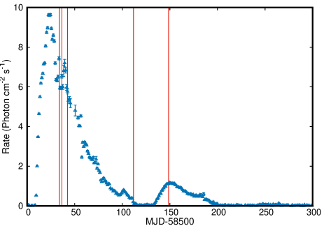
Figure 1: The one-day binned 2–20 keV MAXI light curve of MAXI J1348–630 over the period 2019 January 17 to November 13. The vertical red lines represent AstroSat observations considered in this work.

2.1 AstroSat

We used five publicly available AstroSat (Singh et al., 2014; Agrawal, 2017) Target of Opportunity (ToO) observations of MAXI J1348–630. We marked the observations used in this work on the MAXI light curve, which is shown in Figure 1 and their details are listed in Table 1.

Table 1: Observation Log. (1) Observation data (AS and N represent AstroSat and NICER, respectively); (2) observation ID; (3) date of observation; (4) exposure time (L and S represent LAXPC and SXT, respectively); (5) SXT count rate from a circular region of radius 16 arcmin; (6) inner and outer radius of annulus used for extraction of SXT spectrum. ^aThe SXT data is not piled-up in AS4 observation. Thus, a circular region of radius 16 arcmin is used for event extraction.

Data	ObsID	Date	Exposure	SXT Count Rate	Radius
			(ks)	(c/s)	(arcmin)
AS1	T03_083T01_9000002722	2019 February 19–20	5.5(L)/1.9(S)	879.4	8 & 16
N1	1200530118	2019 February 19	5.0
AS2	T03_083T01_9000002728	2019 February 22	20.2(L)/11.1(S)	844	8 & 16
N2	1200530121	2019 February 22	2.5
AS3	T03_083T01_9000002742	2019 February 28	23.2(L)/12.2(S)	765.7	6 & 16
N3	1200530127	2019 February 28	2.8
AS4	T03_112T01_9000002896	2019 May 8–9	13.8(L)/6.8(S)	13.7	16a
N4	2200530133	2019 May 9	1.9
AS5	T03_120T01_9000002990	2019 June 14–15	35.0(L)/14.9(S)	68.7	2 & 16
N5	2200530154	2019 June 14	1.8
N6	2200530155	2019 June 15	1.6

2.1.1 Large Area X-ray Proportional Counter

LAXPC consists of three proportional counters (LAXPC10, LAXPC20 and LAXPC30) operating in the energy range of 3–80 keV with a temporal resolution of $10\,\rm\mu s$ (Yadav et al., 2016b, a; Antia et al., 2017; Agrawal et al., 2017). We processed the Event Analysis (EA) mode data from these observations using LAXPC software (LaxpcSoft; version as of 2020 August 04). We applied the barycenter correction to the LAXPC level 2 data using the as1bary tool. The standard tools available in LaxpcSoft were used to extract the light curves and energy spectra. The LAXPC10 detector was operating at low gain and the LAXPC30 detector was switched off on 2018 March 8 due to the gas leakage. Thus, we used LAXPC20 detector for our analysis. We modelled the LAXPC20 spectrum in the 5–40 keV energy band.

2.1.2 Soft X-ray Telescope

Soft X-ray Telescope (SXT) is a focussing telescope (Singh et al., 2016, 2017) and all the observations are taken in Photon Counting (PC) mode. SXT has a large time resolution of 2.38 s in PC mode compared to LAXPC. The Level-1 data were processed using the SXT pipeline software (version: AS1SXTLevel2-1.4b) to obtain the cleaned Level-2 event files for each orbit. We merged different orbits data using the SXT event merger tool (Julia based module) and obtained an exposure corrected, merged cleaned event file. The source was piled-up in all observations except AS4 and we removed the pile-up by extracting the source events from annulus region. Different inner radii are used to mitigate the pile-up from SXT data and these radii are given in Table 1. For AS4 observation, we extracted the spectrum from a circular region of radius 16 arcmin. The blank sky SXT spectrum and the redistribution matrix file (sxt_pc_mat_g0to12.rmf) provided by the instrument team were used as the background spectrum and RMF, respectively. The sxtARFModule tool² were used to generate the SXT off-axis auxiliary response files (ARF) using on-axis ARF (sxt_pc_excl00_v04_20190608.arf), provided by the SXT instrument team. While fitting the SXT spectrum, we modified the gain of the response file by the gain command, where the slope is fixed at unity and offset is a free parameter. We used the SXT spectrum in the 0.8–7 keV energy range.

2.2 NICER

NICER (Gendreau et al., 2012) is a payload onboard International Space Station (ISS). The X-ray Timing Instrument (XTI) of NICER comprises of 56 X-ray optics with silicon detectors operating in the 0.2–12 keV energy band (Gendreau et al., 2016). Currently, 52 detectors are active. NICER monitored MAXI J1348–630 from 2019 January 26 immediately after the detection by MAXI/GSC. The source was observed by NICER for more than 300 ks. In this work, we used those NICER observations, which are simultaneous to AstroSat. Hence, we used six NICER observations and their details are given in Table 1. Among them, the observation N2 had telemetry saturation and as a result, the event data was fragmented into very short duration data segments. In this case, we have omitted the MPU0, 3, 4 and 5 and continued our analysis. We have processed the data using heasoft version 6.26.1, NICER software version 2019-06-19_V006a and NICER CALDB version of 20200202 by applying standard filter criteria. We have further excluded detectors #14 and #34 from all observations, which show increased electronic noise occasionally. We examined for the presence of high-energy background flares by extracting the light curve in the 12–15 keV energy band (see Bult et al., 2018). No high background intervals were found in the NICER observations. We use the ftool barycorr to apply the barycenter correction for each NICER observation. Since the source did not show any spectral and intensity variations in the N5 and N6 observations, we combined them for the analysis.

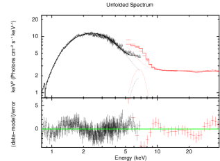
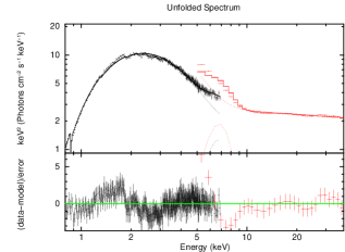
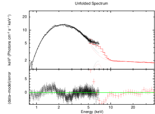
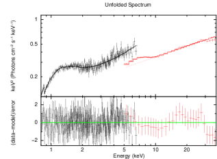
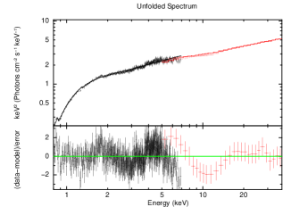
Figure 2: The 0.8–40 keV broadband X-ray spectrum of MAXI J1348–630 from AS1 (top left), AS2 (top middle), AS3 (top right), AS4 (bottom left) and AS5 (bottom right) observations. The black and red data points represent the SXT and LAXPC20 data, respectively. Spectra are fitted with tbabs*(simpl * diskbb + gaussian) model.

Table 2: Broadband X-ray Spectral Parameters for MAXI J1348–630. (1) Observation; (2) segment used; (3) neutral hydrogen column density in units of $10^{22}~{}\rm cm^{-2}$ from tbabs model; (4) photon power law index; (5) scattered fraction; (6) inner disk temperature in keV (7) line energy in keV; (8) line width in keV; (9) gaussian normalization; (10)-(11) the unabsorbed disk flux and total flux in units of $10^{-9}\rm~{}erg~{}cm^{-2}~{}s^{-1}$ in the 0.8–40 keV band derived using cflux; (12) Ratio of the disk flux to the total flux; (13) $\chi^{2}$ statistics and degrees of freedom. In AS2, L and H represent the low and high intensity level segments.

Obs	Seg	$N_{\rm H}$	$\Gamma$	$f$	$\rm kT_{in}$	$E_{line}$	$\sigma$	$\rm N_{gauss}$	$\rm F_{disk}$	$\rm F_{Total}$	$\rm Ratio$	$\rm\chi^{2}/d.o.f$
AS1		$0.54^{+0.01}_{-0.01}$	$2.05^{+0.03}_{-0.03}$	$0.065^{+0.004}_{-0.004}$	$0.799^{+0.007}_{-0.007}$	6.4 (f)	$1.00^{+0.09}_{-0.09}$	$0.107^{+0.012}_{-0.011}$	$32.03^{+0.21}_{-0.21}$	$39.89^{+0.34}_{-0.33}$	0.80	$570.0/395$
AS2		$0.51^{+0.01}_{-0.01}$	$2.12^{+0.03}_{-0.03}$	$0.080^{+0.005}_{-0.005}$	$0.790^{+0.005}_{-0.006}$	6.4 (f)	$1.14^{+0.09}_{-0.09}$	$0.084^{+0.008}_{-0.008}$	$28.64^{+0.16}_{-0.16}$	$36.33^{+0.24}_{-0.23}$	0.79	$743.1/514$
AS2	L	$0.50^{+0.01}_{-0.01}$	$2.03^{+0.03}_{-0.03}$	$0.054^{+0.004}_{-0.003}$	$0.781^{+0.005}_{-0.005}$	6.4 (f)	$1.04^{+0.10}_{-0.10}$	$0.064^{+0.007}_{-0.007}$	$28.08^{+0.16}_{-0.16}$	$33.86^{+0.24}_{-0.24}$	0.83	$688.7/447$
AS2	H	$0.51^{+0.01}_{-0.01}$	$2.19^{+0.03}_{-0.03}$	$0.100^{+0.007}_{-0.006}$	$0.793^{+0.007}_{-0.007}$	6.4 (f)	$1.10^{+0.09}_{-0.09}$	$0.094^{+0.010}_{-0.010}$	$29.22^{+0.19}_{-0.19}$	$38.32^{+0.27}_{-0.27}$	0.76	$676.5/480$
AS3		$0.51^{+0.01}_{-0.01}$	$2.09^{+0.03}_{-0.03}$	$0.078^{+0.005}_{-0.005}$	$0.769^{+0.005}_{-0.005}$	6.4 (f)	$1.14^{+0.07}_{-0.07}$	$0.128^{+0.011}_{-0.010}$	$36.98^{+0.21}_{-0.21}$	$47.45^{+0.31}_{-0.31}$	0.78	$814.9/538$
AS4		$0.39^{+0.03}_{-0.03}$	$1.57^{+0.02}_{-0.02}$	$0.198^{+0.027}_{-0.025}$	$0.277^{+0.015}_{-0.013}$	6.4 (f)	$1.37^{+0.33}_{-0.31}$	$0.005^{+0.002}_{-0.002}$	$0.46^{+0.03}_{-0.03}$	$3.17^{+0.07}_{-0.07}$	0.15	$269.6/300$
AS5		$0.51^{+0.01}_{-0.01}$	$1.55^{+0.01}_{-0.01}$	$0.482^{+0.022}_{-0.031}$	$0.330^{+0.016}_{-0.009}$	6.4 (f)	$1.97^{+0.45}_{-0.33}$	$0.017^{+0.007}_{-0.005}$	$1.66^{+0.08}_{-0.08}$	$18.12^{+0.27}_{-0.19}$	0.09	$551.1/492$

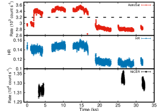
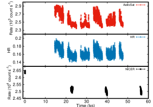
Figure 3: The light curves and hardness ratio from simultaneous AstroSat and NICER observations in the soft state: AS1 & N1 (left), AS2 & N2 (middle) and AS3 & N3 (right). In each plot, the top, middle and bottom panels represent the 3–80 keV light curve from LAXPC20 binned with 10-s, hardness ratio from AstroSat data and 10-s binned light curve in the 0.5-12 keV energy band from NICER observations, respectively. The dashed horizontal line in AS2 observation represents the two flux levels. Hardness ratio is defined as the ratio of the count rate in 7–16 keV and the 3–7 keV bands.

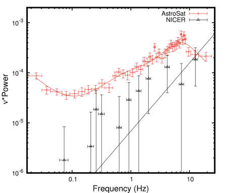
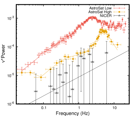
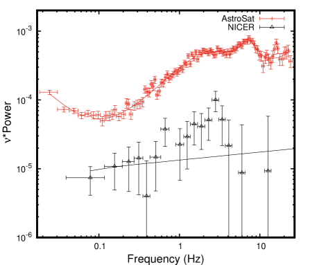
Figure 4: The power density spectrum of MAXI J1348–630 from AstroSat/LAXPC (red plus points) and NICER (black open triangles) observations in the soft state. The observations are AS1 & N1 (top), AS2 & N2 (middle), AS3 & N3 (bottom). In AS2, red plus points and yellow filled circles represent the PDS from the low and high intensity levels in LAXPC light curve (see middle panel of Figure 3). The PDS from AS1 and AS2 are fitted with three Lorentzians, while the AS3 PDS is fitted with four Lorentzians. The NICER PDS are fitted with a power law function.

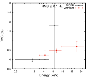
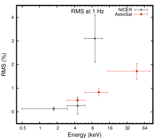
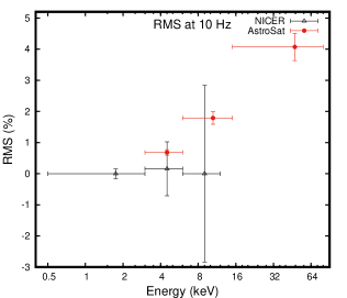
Figure 5: Fractional rms as a function of photon energy in the frequency range 0.08–0.12 Hz (around 0.1 Hz; left), 0.8–1.2 Hz (around 1 Hz; middle) and 8–12 Hz (around 10 Hz; right) from the simultaneous NICER (N1; black open triangle) and AstroSat (AS1; red filled circle) observations in the soft state.

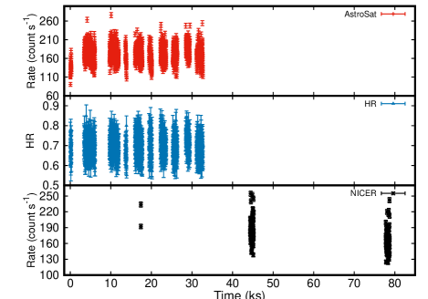
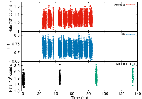
Figure 6: The light curves and hardness ratio from simultaneous AstroSat and NICER observations in the hard state: AS4 & N4 (left) and AS5 & N5 and N6 (right). The labelling is same as that of Figure 3.

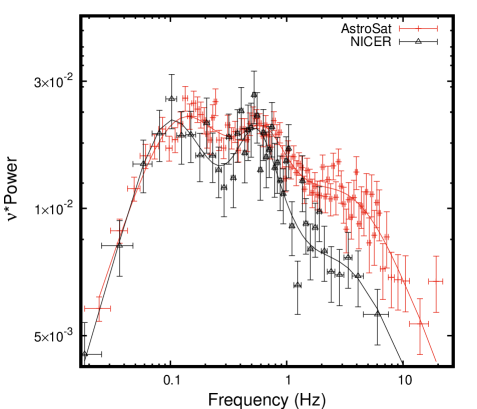
Figure 7: PDS from AS4 (red plus points) and N4 (black open triangles) observations in the faint hard state. Both PDS are fitted with three Lorentzians.

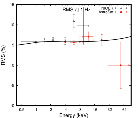
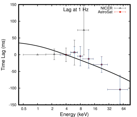
Figure 8: Fractional rms (left) and time lag (right) as a function of photon energy in the frequency range 0.8–1.2 Hz (around 1 Hz) from the faint hard state observation. The red filled circle and black open triangle represent AS4 and N4 observations, respectively. We shifted the time lag detected with AstroSat to the reference band of NICER, which is shown in blue open circles. The black solid curve represents the model fit derived from the stochastic propagation model.

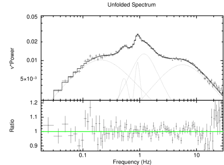
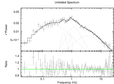
Figure 9: PDS from AS5 (left), N5 and N6 (right) observations in the bright hard state, which are fitted with five Lorentzians. For the NICER PDS, we fixed the centroid frequency and width of all the Lorentzian functions to the best-fit values obtained from the AstroSat PDS.

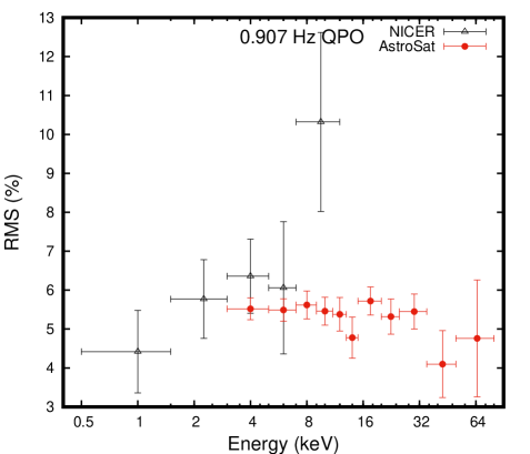
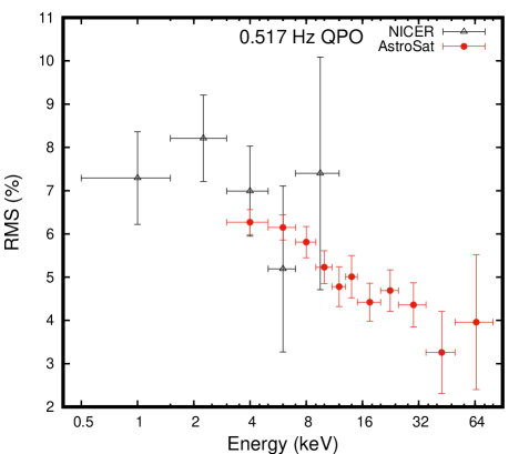
Figure 10: Fractional rms as a function of photon energy at 0.907 Hz QPO (left) and 0.517 Hz sub-harmonic (right) from the AS5 (red filled circle) and NICER (N5 and N6; black open triangle) observations.

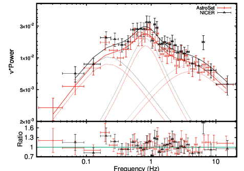
Figure 11: The PDS from the strict overlapping time between AstroSat (AS5) and NICER (N5) observations in the common energy range of 3–6 keV fitted with three Lorentzians. The red plus points and black open triangles represent AstroSat and NICER data, respectively.

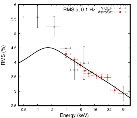
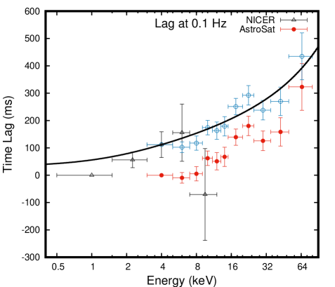
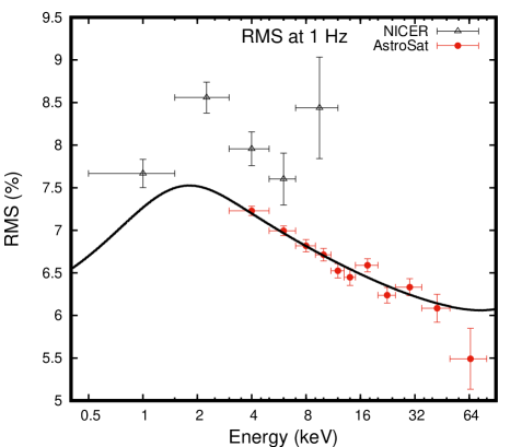
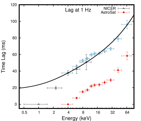
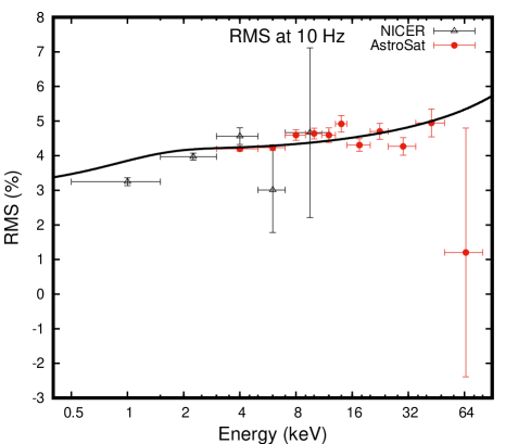
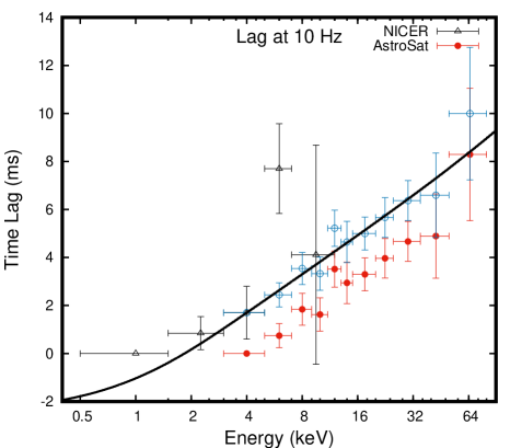
Figure 12: Fractional rms (left) and time lag (right) as a function of photon energy at 0.08–0.12 Hz (0.1 Hz; top panel), 0.8–1.2 Hz (1 Hz; middle panel) and 8–12 Hz (10 Hz; bottom panel) frequencies from the simultaneous AS5 (red filled circle) and NICER (N5 and N6; black open triangle) observations. The LAXPC time lags have been shifted such that the 3–5 keV time lag is same as for NICER and is shown in blue open circles. The black solid curve represents the model fit derived from the stochastic propagation model.

3 Broadband X-ray Spectral Analysis

We first performed the broadband X-ray spectral analysis of MAXI J1348–630 using the SXT and LAXPC instruments onboard AstroSat. The broadband spectrum in the 0.8–40 keV energy band were modelled with xspec version 12.10.1f (Arnaud, 1996). Here our motivation is to understand the spectral state of source and hence we used a simple model for the broadband spectral modelling, which consists of a multi-colour disk blackbody (MCD; diskbb in xspec; Mitsuda et al., 1984) and a Comptonization component (simpl; Steiner et al., 2009) along with a gaussian line profile (gaussian). Detailed spectral modelling taken into account relativistic effects will be presented elsewhere. We used Tuebingen-Boulder Inter-Stellar Medium absorption model (tbabs; Wilms et al., 2000). A multiplicative constant was used to address the cross-calibration uncertainties between the SXT and LAXPC instruments. A 3% model systematic uncertainty is used for spectral modelling. The parameter errors are at a 90% confidence level.

The unfolded spectra and residuals from the five observations are depicted in Figure 2 and the best-fit model parameters are listed in Table 2. The absorption column density seems to be a constant at $\sim 5\times 10^{21}~{}\rm cm^{-2}$ for these observations, except in AS4 observation, where it dropped to $\sim 4\times 10^{21}~{}\rm cm^{-2}$. The photon index, scattering fraction and inner disk temperature significantly changed during these observations. The photon index decreases from $\sim 2.1$ to $\sim 1.6$, while the scattering fraction increases from $\sim 7\%$ to $\sim 50\%$. The inner disk temperature shows a decreasing trend from $\sim 0.8$ to $\sim 0.3$ keV. The unabsorbed flux was computed using the convolution model cflux in the 0.8–40 keV energy band. The total flux increases from $\sim 4$ to $\sim 4.7\times 10^{-8}\rm~{}erg~{}cm^{-2}~{}s^{-1}$ in the first three observations. In the AS4 observation, the flux drops by a factor $\sim 15$ compared to AS3 observation and then increases to $\sim 2\times 10^{-8}\rm~{}erg~{}cm^{-2}~{}s^{-1}$ in the last AstroSat (AS5) observation.

In the first three observations (AS1, AS2 and AS3), the value of power law index is $>2$, the inner disk temperature $\sim 0.8$ keV, the scattered fraction of seed photon from the accretion disk is $\lesssim 10\%$ and estimated disk fraction is $>75\%$, which identifies the source to be in the soft spectral state of BHXRBs. The X-ray spectrum of the source significantly changed in the last two observations (AS4 and AS5), with photon index $\sim 1.6$, the inner disk temperature dropped to $\sim 0.3$ keV, the scattered fraction of $\sim 20-50\%$ and disk fraction dropped below 15%. Based on the spectral parameters, we have identified the source to be in the hard X-ray spectral state of BHXRBs (Remillard & McClintock, 2006; Belloni, 2010; Belloni et al., 2011) in these observations. In the next section, we discuss the broadband time variability. We first consider the three soft state observations and then the two hard state ones.

4 Broadband Timing Analysis

4.1 Soft State Observations

The AstroSat LAXPC20 background subtracted 3–80 keV light curves of MAXI J1348–630 in the soft state (AS1, AS2 and AS3) are depicted in the top panels of Figure 3. In the AS2 observation, the intensity increased from $\sim 3000~{}\rm count~{}s^{-1}$ to $\sim 3400\rm~{}count~{}s^{-1}$ in a short period and then the source flipped back to the lower intensity level. The hardness ratio (HR) is defined as the ratio between the 7–16 keV and the 3–7 keV rate and its variation is shown in the middle panels of Figure 3. The 0.5–12 keV light curves from NICER observations, which are simultaneous to AstroSat are plotted in the bottom panels.

The power density spectrum (PDS) in the 0.01–30 Hz frequency range from LAXPC and NICER data for the energy range 3–15 keV and 0.5–12 keV, respectively, are shown in Figure 4. The LAXPC PDS shows complex broad band features and require to be fitted by multiple Lorentzians. Since the source exhibited different intensity levels in the LAXPC light curve of AS2 observation, we extracted the PDS from low and high-intensity levels which are shown in the middle panel of Figure 4. The PDS from the low and high intensity levels are different and the PDS becomes weaker in the high-intensity level compared to the lower one. In addition, we can see a broad feature (the centroid frequency is $\sim 4.6$ Hz and the width is $\sim 4.3$ Hz) appeared in the PDS extracted from the high intensity level. In the PDS of AS3 observation, we can see a QPO at $6.85^{+0.24}_{-0.26}$ Hz with a width $3.80^{+0.85}_{-0.74}$ Hz. The detected QPO at $\sim 6.9$ Hz is broad (the $Q$-factor is $\sim 1.8$) and the rms is $<2\%$ in the AstroSat energy bands.

In contrast, the PDS obtained from NICER data shows significantly lower values and hence can be modelled using a simple power-law as shown in Figure 4. The difference in variability between the NICER and LAXPC suggests a strong energy dependence of the fractional rms. To verify if that is the case, we extracted the fractional rms, by following the methods discussed in Nowak et al. (1999), as a function of energy, for three frequency ranges (0.08–0.12, 0.8–1.2 and 8–12 Hz) for the first observation (AS1 and N1) and plotted them in Figure 5. We note that for the common energy range of 3–5 keV the NICER and LAXPC fractional rms are consistent with each other. The variability is more pronounced at higher energies reflecting a larger fractional rms in the LAXPC bands. We have also computed the time lag at three frequency ranges using several energy bands from NICER and AstroSat. To compute the time lag, we used 0.5–3 keV (NICER) and 3–6 keV (AstroSat) as the reference energy bands in the AS1, AS2, AS3 and corresponding NICER observations. We do not observe any trend in the time lag spectra, hence those lag spectra are not shown in the paper.

In §3, spectral analysis of the soft state data revealed that the disc emission dominates for energies $<4$ keV as is seen in the top three panels of Figure 2. Thus, the prominent variability observed in LAXPC data and a significantly reduced variability in the NICER one, can be understood in the framework where the disk emission is non-variable while the Comptonized component rapidly varies. While this has been inferred from earlier temporal analysis of black hole systems in the soft state, here we confirm the results using broadband spectral and timing analysis.

4.2 Hard State Observations

For the two hard state observations (AS4, AS5 and corresponding NICER observations) the intensity varied significantly between the observations, although the hardness ratio remained similar for both (see Figure 6). There were no significant flux variations seen in the light curves of each of the observations. The difference in the intensity prompted us to name the data set AS4 and N4 as belonging to the faint hard state and the AS5 and corresponding NICER observations as the bright hard state. We study the rapid variability of these two states separately in the next two sub-sections.

4.2.1 Faint Hard State

The power density spectra for the faint hard state observations show broad features in the 0.01–30 Hz frequency range with no QPOs. In contrast to the soft state observations described in the previous section, the PDS are similar in the low energy (NICER) and high energy (LAXPC) data. Figure 7 shows the PDS generated from LAXPC data in the 3–15 keV along with that generated from NICER data in the 0.5–12 keV range. Three broad Lorentzians have been used to model both the data sets.

To explore the energy dependence further, we extracted the fractional rms at three frequency ranges 0.08–0.12, 0.8–1.2 and 8–12 Hz, as was done for the soft state observations. The rms seems to be a constant around $\sim 7\%$ and the time lags are consistent with zero at $\sim 0.1$ and $\sim 10$ Hz. Thus, we show the rms and lag spectrum for the frequency range 0.8–1.2 Hz, from both NICER and LAXPC data in Figure 8. The variability seems to be nearly a constant at $\sim 7$% over all energies. There is a slight discrepancy at the common energy range of 5–7 keV for NICER and LAXPC data, but the deviation is within two sigma and moreover the data are not strictly simultaneous (see Figure 6). The time lag versus energy for the same frequency range is shown in the right panel of Figure 8. Here the reference energy band for the NICER data is 0.5–1.5 keV while for LAXPC it is 3–5 keV. While there is no significant time lag for the NICER data, there is a soft lag at high energies for LAXPC data of the order of 100 ms. Such a soft lag is rather unusual for the hard state of black hole binaries.

4.2.2 Bright Hard State

After the main outburst, the source exhibited a re-flare which peaked around MJD 58648 (see Figure 1). The source’s intensity increased to $\sim 1300\rm~{}count~{}s^{-1}$ in the bright hard state observation (AS5) compared to the earlier hard state observation where the count rate was $\sim 200\rm~{}count~{}s^{-1}$. The higher count rate allows for a more detailed timing analysis.

The PDS obtained from LAXPC in the 3–15 keV energy band is shown in the left panel of Figure 9. The PDS can be described by five Lorentzian functions which represent three broadband components along with a QPO at $0.907\pm 0.01$ Hz ($Q$-factor $\sim 4.7$) and a possible sub-harmonic at $0.517\pm 0.02$ Hz ($Q$-factor $\sim 2.4$) with widths $0.194\pm 0.06$ Hz and $0.223\pm 0.07$ Hz, respectively. Here, the Lorentzian component with the higher $Q$-factor is considered to be the primary QPO, while the other one is taken to be the sub-harmonic. Indeed, the temporal behaviour of the systems at $\sim 1$ Hz is complex, with a broader component peaking at $\sim 1.5$ Hz close to the QPO feature. The fitting resulted in a formal $\chi^{2}$/dof$=160.6/93$.

The right panel of Figure 9 shows the PDS generated from the NICER observations in the energy range 0.5–12 keV. The overall shape of the PDS is similar to that obtained from LAXPC but with changes in relative strengths of the components. This is demonstrated by fitting the same five Lorentzian as used for LAXPC data for the NICER one. Here, the centroid frequency and width of the Lorentzian components are fixed to the values obtained for the LAXPC fitting, but allowing for the normalization to vary. This leads to an acceptable $\chi^{2}$/d.o.f $=93.3/98$. While the QPO components seems to have nearly the same strength for both observations, the sub-harmonic component normalization is lower for LAXPC data. To quantify the energy dependence of the QPO features, the PDS at different energies were fitted with the same five component model and the normalization of the Lorentzians was used to determine the fractional rms. The results are illustrated in Figure 10, where the left panel shows that strength of the primary QPO is nearly energy independent, while for the sub-harmonic it decreases with energy.

The slight difference in the temporal behaviour seen between the NICER and LAXPC analysis could be either due to the different energy band used for the two instruments or it could be that the source behaviour changed for the two observations, since they are not strictly simultaneous. To check for these possibilities, PDS was generated for the small $\sim 500$ seconds strict simultaneous data available for both instruments (see right panel of Figure 6) in the common energy range of 3–6 keV. Figure 11 shows the two strict simultaneous PDS, which shows that the overall shape of the PDS from the two instruments are remarkably similar, with the NICER data showing a slight higher variability. The slightly lower PDS values for the LAXPC data may be due to dead time effects. While dead time corrections have been incorporated in the Poisson level of the LAXPC data (Yadav et al., 2016a), the real variability strength may be slightly smaller due to dead time which has not been taken into account here. Both the PDS can be represented by three Lorentzian components. Unfortunately, the QPOs and the complex features seen at 1 Hz, are not distinguishable here for this short time observation. Thus, while Figure 11 illustrates how well the analysis of two instruments agree with each other, it is not clear whether the slight variation seen in the PDS in Figure 9 for the LAXPC and NICER data is due to energy dependence or source variation. Nevertheless, we continue with further energy-dependent temporal analysis of the data keeping in mind that the data is not strictly simultaneous.

Since the statistics are not good enough to ascertain the detailed energy-dependent properties such as time lag for the QPO and other individual features we study the energy-dependent temporal properties of the source in three broad frequency bands. Figure 12 shows the fractional rms and time lag as a function of energy for the frequency ranges 0.08–0.12 Hz (around 0.1 Hz), 0.8–1.2 Hz (around 1 Hz) and 8–12 Hz (around 10 Hz). The reference energy bands for the time lag computation is 0.5–1.5 keV and 3–5 keV for the NICER and LAXPC bands, respectively. Also shown in the right panel (with blue open circles) the LAXPC time lag shifted such that the 3–5 keV time lag is the same as that observed by NICER. Hence these data points can be considered to be having the same reference energy band as that of NICER i.e. 0.5–1.5 keV. To further understand the frequency-dependent time lag, we extracted the frequency-dependent time lags between 3–4 keV and 4–12 keV energy band for the bright hard state observation and shown in Figure 13. A hard time lag has been observed at all frequencies in this observation, which is consistent with time lag spectra extracted from three frequency ranges.

Figure 13: Frequency-dependent time lags between 3–4 keV and 4–12 keV band light curves from AS5 observation.

Broadly, the rms is seen to decrease with energy for $\sim 0.1$ and $\sim 1$ Hz, while for $\sim 10$ Hz there is a marginal increase with energy. The magnitude of the time lags depend on the frequency range and are found to be hard lags i.e. the lags increase with energy. Note the apparent difference in nature of the rms versus energy when a broad frequency range is taken around 1 Hz (right middle panel of Figure 12) as compared to when it is estimated only for the QPO at 0.91 Hz (left panel of Figure 10), although the errors are larger for the QPO. This indicates the complexity of the temporal behaviour of the system at around 1 Hz.

In the next section we model and interpret the energy-dependent rms and time lag at different frequencies in terms of a single-zone stochastic propagation model applicable for the hard state of black hole binaries.

5 Modelling the Energy Dependent Timing Properties

One of the promising models to explain the timing properties of BHXRBs is the stochastic propagation one (Lyubarskii, 1997; Kotov et al., 2001; Ingram & Done, 2011, 2012; Ingram & van der Klis, 2013). In this interpretation variability induced in the outer regions of the disk, at different frequencies, propagate inwards to produce the observed variability in the X-ray band. Different versions of this generic scenario can be invoked to predict the fractional rms and time lag as a function of energy. Maqbool et al. (2019) have described in detail a single-zone stochastic propagation model which they used to fit the energy-dependent timing properties of Cygnus X–1. This model has also been successfully used to fit the energy-dependent timing features of the broadband noise in MAXI J1820+070 (Mudambi et al., 2020) and of the QPO in Swift J1658.2$-$4242 (Jithesh et al., 2019).

While details of the single-zone propagation model are presented in Maqbool et al. (2019), here we briefly mention some of the primary components. The assumed geometry of the system is a truncated standard disk characterised by a inner disk temperature $T_{\rm in}$, with a hot inner flow having a single uniform temperature $T_{\rm e}$, hence the model is termed as a single-zone one. The inner flow Compontonizes photons from the truncated disk to produce the observed hard X-ray emission. Variations in the inner disk temperature $\delta T_{\rm in}$, changes the input photons inducing a variation in the Comptonized spectrum. Additionally, there is a variation in the heating rate of the hot inner flow inducing a variation in its temperature $\delta T_{\rm e}$, which can occur after a time delay compared to $\delta T_{\rm in}$.

The model requires the parameters of the Comptonized component obtained from the time averaged spectrum, namely the inner disk temperature, the power-law index and the temperature of the hot inner region. The first two are estimated directly by the spectral fitting described in Section 3 (see Table 2). Since the temperature of the hot inner region cannot be constrained by the spectral fitting we assume it to be $100$ keV. The other parameters required are the variation $\delta T_{\rm e}$, the ratio $\delta T_{\rm in}/\delta T_{\rm e}$ and the time delay between them $\tau_{D}$.

Since the model is applicable only to the thermal Comptonized component, we restrict the analysis only to the hard state data. Furthermore, we only formally fit the LAXPC data in the energy range (3–80 keV) and extrapolate the predicted variability to low energies to compare with the NICER results. The best-fit parameters are listed in Table 3 and the model is plotted as black solid line in Figures 8 and 12. For the time lag curves, the model prediction are shifted such that the time lag at 3–5 keV matches with the observed NICER values and hence can be interpreted as being the time lag with reference to 0.5–1.5 keV band.

For the bright hard state observation, the model predictions match well with the LAXPC observations for frequencies $\sim 0.1$ and $\sim 10$ Hz, with reduced $\chi^{2}_{r}=0.8$ and $1.2$, respectively. For several observations of Cygnus X–1 the best-fit parameters of $\delta T_{\rm e}$, $\delta T_{\rm in}/\delta T_{\rm e}$ and $\tau_{D}$ range from 0.005–0.03, 0.6–1.8 and 70–300 ms for $\sim 0.1$ Hz while for $\sim 10$ Hz the corresponding ranges are 0.015–0.03, 0.3–0.6 and 2–9 ms (Maqbool et al., 2019). For MAXI J1820+070, the values obtained are $\sim 0.03$, $\sim 1.2$ and $\sim 500$ ms for $0.1$ Hz and $\sim 0.03$, $\sim 0.6$ and $\sim 6$ ms for 10 Hz. The parameter values obtained in this work for MAXI J1348–630 are in the same range as the above (Table 3). Extending the time lag model predictions to lower energies shows a reasonable match with the NICER results for 0.1 and 10 Hz (Right top and bottom panels of Figure 12). For the rms variation, NICER results are above the predictions for 0.1 Hz while for 10 Hz there is an under prediction. Note that the model predicts a turnover at $\sim 2$ keV, and hence NICER data in principle should be able verify the prediction. However, we caution against over interpretation since the NICER and LAXPC results are not strictly simultaneous and more importantly, the model is only applicable to the Comptonized component and at these low energies the disk emission could be important.

For the results corresponding to $\sim 1$ Hz, the model fit is not acceptable with $\chi^{2}_{r}=2.9$, although the parameters obtained are similar to what has been estimated for Cygnus X–1. An inspection of the LAXPC results show that the energy-dependent time lag (middle right panel of Figure 12) is well constrained with relatively smaller error bars and has a monotonic behaviour with an inflection point around 20 keV. This complexity is not captured by the model which predicts only smooth behaviour. This behaviour could be generic and has been brought out due to better statistics at $\sim 1$ Hz or it could be due to the presence of the QPO at $\sim 0.91$ Hz which may have a different temporal behaviour than the broadband noise. Extension of the model prediction of the time lag to lower energies shows a clear mismatch with NICER results and the predicted rms is lower than what is observed (middle panel of Figure 12). Interestingly, there is a turnover at $\sim 2$ keV for the NICER results as predicted by the model but at a higher rms level. Again for reasons mentioned above, we caution against over interpreting comparison of the NICER results with the extension of the model to lower energies.

For the faint hard state the statistics are not good enough to perform detailed modelling of the energy-dependent variability. Nevertheless, we modelled the fractional rms and time lag for the LAXPC data for frequency range 0.8-1.2 Hz. The best-fit models are shown as solid lines in Figure 8 and parameters are listed in Table 3. It is interesting to note that the parameter values are similar to those obtained for the bright hard state data for the same frequency range, except that the time delay $\tau_{D}$ is negative. A negative $\tau_{D}$ means that the soft photon source variation $\delta T_{in}$ occurred after the variation in the coronal temperature $\delta T_{e}$ which implies that the variability originates in the corona and propagates outward in contrast to the more standard propagating model interpretation used for the bright hard state in this work, as well as for Cygnus X–1 (Maqbool et al., 2019) and MAXI J1820+070 (Mudambi et al., 2020). Indeed, an identical outward propagating interpretation was invoked by Jithesh et al. (2019) to explain the soft lags observed for the QPO in Swift J1658.2-4242 in its hard intermediate state. However, it should be emphasised that the significance of the time lag measurement in the LAXPC data of the faint state is not as high as that it is for the high flux hard state data.

Table 3: Best-fit Parameters from the Stochastic Propagation Model. (1) Spectral state (F and B represent the faint and bright hard state, respectively); (2) Frequency range in Hz; (3) ratio of the variation in the inner disk temperature to the variation of electron temperature; (4) time lag in ms; (5) variation in the electron temperature; (6) $\chi^{2}$ statistics and degrees of freedom.

State	Freq	$\delta T_{\rm in}/\delta T_{\rm e}$	$\tau_{D}$	$\delta T_{\rm e}$	$\rm\chi^{2}_{r}/d.o.f$
F	0.8-1.2	$0.61^{+0.97}_{-0.32}$	$-93.46^{+61.75}_{-56.98}$	$0.025^{+0.013}_{-0.013}$	0.6/7
B	0.08-0.12	$1.09^{+0.10}_{-0.09}$	$342.26^{+60.77}_{-60.51}$	$0.011^{+0.001}_{-0.001}$	0.8/17
	0.8-1.2	$0.86$	$71.86$	$0.024$	2.9/17
	8-12	$0.52^{+0.05}_{-0.05}$	$9.07^{+1.21}_{-1.23}$	$0.021^{+0.001}_{-0.001}$	1.2/17

6 Summary and Discussion

In this work, we have presented the broadband spectral-timing analysis of the new black hole binary candidate MAXI J1348–630 using simultaneous AstroSat and NICER observations. The main results of the study are summarized below.

• The broadband spectral analysis (in the 0.8–40 keV energy) of the five AstroSat observations identified the source to be in the soft spectral state for the first three observations and in the hard state for the last two observations. The two hard state observations differ significantly in flux and hence were named as faint and bright hard states. The soft state spectra are disk emission dominated with a high energy power-law index $\sim 2$, while the hard state spectra are dominated by Comptonized emission with power-law index $\sim 1.55$.

• In one of the soft state AstroSat observations a weak ($<2\%$ rms), broad ($Q<2$) QPO is detected with a centroid frequency of $\sim 6.9$ Hz. This low frequency QPO most likely belongs to the class of type-A QPOs (Casella et al., 2004; Belloni et al., 2011; Motta, 2016). Another QPO with a sub-harmonic feature, was detected in the bright hard state observation, with centroid frequency $\sim 0.9$ Hz, variability amplitude $\sim 6$% and a Q factor of $\sim 4.7$. From these properties, we identify this QPO as a type-C QPO (Casella et al., 2004; Casella et al., 2005; Motta et al., 2015).

• For the first time, we estimated the energy-dependent fractional rms and time lag of MAXI J1348–630 in the 0.5–80 keV energy band using the NICER/XTI and AstroSat/LAXPC instruments for a range of frequencies and for the QPOs.

• In the soft state observations, the power density spectra (computed in the 0.01–30 Hz frequency range) for the 0.5–12 keV NICER band is significantly lower by at least a factor of $\sim 5$ from that of the 3–80 keV AstroSat LAXPC. This is further illustrated by computing the energy dependence of the fractional rms at different frequencies, which show an increasing trend with energy. Based on the spectral fitting, this implies that the variability in the soft state is dominated by the hard X-ray Comptonized component and the disk emission is significantly less variable.

• For the bright hard state observation, fitting the power density spectra with Lorentzian functions, revealed that the fractional rms of the Lorentzian representing the QPO at $\sim 0.9$ Hz is nearly energy independent at $\sim 5$%, while a decreasing trend with energy is seen for the sub-harmonic. However, when the fractional rms is estimated from the PDS directly in a broad frequency range of 0.8–1.2 Hz a clear decrease with energy is detected. Moreover, the fractional rms is different for NICER and LAXPC data even in the same energy band. This implies that the temporal features around $\sim 1$ Hz is complex with the presence of a weak QPO along with broad band noise. The inconsistency between the NICER and LAXPC fractional rms estimation can be due to variation of the source’s temporal property at $\sim 1$ Hz during the observation. Strictly simultaneous PDS generated from NICER and LAXPC show similar shapes although the statistics are low due to the smaller exposure time. The fractional rms in the frequency ranges of 0.08–0.12 and 8.0–12.0 Hz decreased and moderately increased with energy, respectively and the NICER and LAXPC data points were consistent with each other in the common energy range.

• For the bright hard state observation, hard time lags (i.e. time lags increasing with energy) are clearly detected at $\sim 0.1$, $1$ and $10$ Hz in the unprecedented energy range of 0.5–80 keV. The time lag between 60 keV and 1 keV photons varies with frequency such that it is $\sim 400$, $\sim 80$ and $\sim 8$ milli-seconds at $\sim 0.1$, $1$ and $10$ Hz, respectively. At $\sim 1$ Hz the time lag shows monotonic behaviour with an inflection point around 20 keV which may be related to the complexity of having a weak QPO along with broad band noise in that frequency range.

• For the faint hard state observation, the PDS of the NICER and LAXPC observations were found to be similar with enhanced variability in the higher energy LAXPC band for frequencies $>2$ Hz. Soft time lag (i.e. time lag decreasing with energy) was detected in the LAXPC band at $\sim 1$ Hz.

• We fitted the energy-dependent fractional rms and time lags using a simple single-zone stochastic propagation model (Maqbool et al., 2019). The model is parametrized by variation in the input seed photon temperature ($\delta T_{in}$), the coronal electron temperature ($\delta T_{e}$) and the time lag between them ($\tau_{D}$). It requires the time averaged spectral parameters of the Comptonization component and is valid only when the time averaged spectrum is dominated by the Comptonization component. The model describes the LAXPC 3–80 keV data well for the bright hard state for frequencies $\sim 0.1$ and $\sim 10$ Hz, but fails to fit the monotonic nature of the time lag at $\sim 1$ Hz. The parameters obtained are similar to the ones obtained from fitting the energy-dependent fractional rms and time lags of Cygnus X–1 and MAXI J1820+070 (Maqbool et al., 2019; Mudambi et al., 2020). For the faint hard state the soft lags require that $\tau_{D}$ to be negative i.e. the coronal temperature varies before the seed photon one.

• Extending the single-zone stochastic model fitted to LAXPC data to lower energies, we find that the predicted rms and time lag are qualitatively similar but quantitatively different from NICER results, especially at $\sim 1$ Hz. This discrepancy could be because the NICER and LAXPC data are not strictly simultaneous and/or the model does not take into account disk emission which contributes in the low energy band.

The QPO detections presented here are consistent with previous studies of the source with NICER observations (Zhang et al., 2020). However, NICER also detected a $\sim 7$ Hz type-A QPO in four data segments five days after the AS3 observation (Zhang et al., 2020). In addition, a strong type-B QPO at $\sim 4.5$ Hz in the SIMS was a detected in a set of NICER observations (Belloni et al., 2020). Unfortunately, AstroSat did not observe the source during these times.

It is known that the variability is weak in the soft state of BHXRBs (e.g. Motta, 2016) and that the disk emission is significantly less variable than the Comptonized one. However, with LAXPC and NICER observations we could measure the variability across a wide range of energies and hence confirm that the emission below 4 keV is significantly less variable than that for higher energies. Moreover, spectral analysis revealed that indeed the disk emission contributes significantly below 4 keV.

Rapid repeated flux variations have been detected in a handful of black hole X-ray transients during their outburst, which are generally referred to as flip flops (Miyamoto et al., 1991; Takizawa et al., 1997; Sriram et al., 2012; Bogensberger et al., 2020; Buisson et al., 2021). These flip flops are characterised by an abrupt change in flux with transition time scales ranging from few tens to more than 1 ksec (Miyamoto et al., 1991; Takizawa et al., 1997; Homan et al., 2001; Homan et al., 2005). They occur in the intermediate state and exhibit rapid transitions between different types of QPOs. On some occasions, significant changes in spectral parameters have been observed (Bogensberger et al., 2020), although for others the spectral parameters remain unchanged (Miyamoto et al., 1991). Here, for MAXI J1348–630, we have seen a reminiscent of flip-flops in one of the AstroSat observations (AS2; see middle panel of Figure 3). It is interesting to note that this rare phenomenon is observed here in the soft state and we do not detect QPOs in the bright and dim phases of flip flops in contrast to previous studies. However, there is evidence for a broad feature in the PDS extracted from the high-intensity level (see middle panel of Figure 4). Moreover, for MAXI J1348–630, we do observe changes in the spectral parameters similar to previously detected flip flops. In particular the photon index, scattering fraction and the inner disk temperature change during the flip flop event.

AstroSat observations provide simultaneous spectral coverage from 0.8–40 keV along with energy-dependent fractional rms and time lag in the 3–80 keV band, for a range of Fourier frequencies. This has allowed to test a physical (albeit simple) fluctuation model and to obtain physical parameters (Maqbool et al., 2019). For the hard state of Cygnus X–1, the physical parameters consisting of variation of inner disk temperature, coronal temperature and the time-delay between them varied for different observations (Maqbool et al., 2019). The same model could also explain the timing features of MAXI J1820+070 in the hard state (Mudambi et al., 2020). While the above analysis were undertaken for the continuum variability, the model has also been applied to a QPO observed in Swift J1658.2–4242 (Jithesh et al., 2019), where soft instead of hard time lags were seen. This implied that for the QPO in Swift J1658.2–4242, the coronal temperature varied before the inner disk one, which in turn suggests that the variability is propagating in the outward direction. Here, we show that for the bright hard state of MAXI J1348–630, the model fits the data for $\sim 0.1$ and $\sim 10$ Hz, but deviations are seen for $\sim 1$ Hz. The parameter values obtained are similar to the ones obtained for Cygnus X–1 and MAXI J1820+070. For the faint hard state data, soft lags are observed and hence model fitting reveals coronal temperature variation earlier than the inner disk one, similar to the results obtained for the QPO in Swift J1658.2–4242.

NICER data allows for verifying the model predictions at energies lower than 4 keV. We find that while there is qualitative similarity between the model predictions and NICER measurements of the fractional rms and time lags, there are quantitative differences. It is important to note that the model used in this work is only valid for the thermal Comptonized component. The presence of disk emission at these energies would need to be considered. A more sophisticated model incorporating the disk emission has been formulated and applied to the energy-dependent variability of a QPO of GRS 1915+105 (Garg et al., 2020). However, since the source’s rapid temporal behaviour may vary in time-scales of hours, such models can be applied with confidence only to strictly simultaneous NICER and AstroSat observations.

It should be emphasized that the data used in this work from NICER and AstroSat are not from a coordinated observation between the missions. Hence, the strictly simultaneous data from the two mission is sparse which has limited the analysis. This underlines the need for joint coordinated observations between NICER and AstroSat in the future, which would be critical for our understanding of the broadband spectral-timing properties of X-ray binaries.

Data Availability

The data used in this article are available in the ISRO’s Science Data Archive for AstroSat Mission (https://astrobrowse.issdc.gov.in/astro_archive/archive/Home.jsp) and HEASARC database (https://heasarc.gsfc.nasa.gov). The source code for the model used in the paper can be shared on reasonable request to the corresponding author, V. Jithesh (email: vjithesh@iucaa.in or jitheshthejus@gmail.com).

References

- Agrawal (2017) Agrawal P. C., 2017a, Journal of Astrophysics and Astronomy, 38, 27
- Agrawal et al. (2017) Agrawal P. C., et al., 2017b, Journal of Astrophysics and Astronomy, 38, 30
- Antia et al. (2017) Antia H. M., et al., 2017, ApJS, 231, 10
- Arnaud (1996) Arnaud K. A., 1996, in Jacoby G. H., Barnes J., eds, Astronomical Society of the Pacific Conference Series Vol. 101, Astronomical Data Analysis Software and Systems V. p. 17
- Baby et al. (2020) Baby B. E., Agrawal V. K., Ramadevi M. C., Katoch T., Antia H. M., Mandal S., Nand i A., 2020, MNRAS, 497, 1197
- Belloni (2005) Belloni T., 2005, in Burderi L., Antonelli L. A., D’Antona F., di Salvo T., Israel G. L., Piersanti L., Tornambè A., Straniero O., eds, American Institute of Physics Conference Series Vol. 797, Interacting Binaries: Accretion, Evolution, and Outcomes. pp 197–204 (arXiv:astro-ph/0504185), doi:10.1063/1.2130233
- Belloni (2010) Belloni T. M., 2010, States and Transitions in Black Hole Binaries. p. 53, doi:10.1007/978-3-540-76937-8_3
- Belloni et al. (2011) Belloni T. M., Motta S. E., Muñoz-Darias T., 2011, Bulletin of the Astronomical Society of India, 39, 409
- Belloni et al. (2019) Belloni T. M., Bhattacharya D., Caccese P., Bhalerao V., Vadawale S., Yadav J. S., 2019, MNRAS, 489, 1037
- Belloni et al. (2020) Belloni T. M., Zhang L., Kylafis N. D., Reig P., Altamirano D., 2020, MNRAS, 496, 4366
- Bhargava et al. (2019) Bhargava Y., Belloni T., Bhattacharya D., Misra R., 2019, MNRAS, 488, 720
- Bogensberger et al. (2020) Bogensberger D., et al., 2020, A&A, 641, A101
- Buisson et al. (2021) Buisson D. J. K., et al., 2021, MNRAS, 500, 3976
- Bult et al. (2018) Bult P., et al., 2018, ApJ, 859, L1
- Casella et al. (2004) Casella P., Belloni T., Homan J., Stella L., 2004, A&A, 426, 587
- Casella et al. (2005) Casella P., Belloni T., Stella L., 2005, ApJ, 629, 403
- Chen et al. (2019) Chen Y. P., et al., 2019, The Astronomer’s Telegram, 12470, 1
- Denisenko et al. (2019) Denisenko D., et al., 2019, The Astronomer’s Telegram, 12430, 1
- Garg et al. (2020) Garg A., Misra R., Sen S., 2020, MNRAS, 498, 2757
- Gendreau et al. (2012) Gendreau K. C., Arzoumanian Z., Okajima T., 2012, in Takahashi T., Murray S. S., den Herder J.-W. A., eds, Society of Photo-Optical Instrumentation Engineers (SPIE) Conference Series Vol. 8443, Space Telescopes and Instrumentation 2012: Ultraviolet to Gamma Ray. p. 844313, doi:10.1117/12.926396
- Gendreau et al. (2016) Gendreau K. C., et al., 2016, in den Herder J.-W. A., Takahashi T., Bautz M., eds, Society of Photo-Optical Instrumentation Engineers (SPIE) Conference Series Vol. 9905, Space Telescopes and Instrumentation 2016: Ultraviolet to Gamma Ray. p. 99051H, doi:10.1117/12.2231304
- Homan et al. (2001) Homan J., Wijnands R., van der Klis M., Belloni T., van Paradijs J., Klein-Wolt M., Fender R., Méndez M., 2001, ApJS, 132, 377
- Homan et al. (2005) Homan J., Miller J. M., Wijnands R., van der Klis M., Belloni T., Steeghs D., Lewin W. H. G., 2005, ApJ, 623, 383
- Homan et al. (2020) Homan J., et al., 2020, ApJ, 891, L29
- Ingram & Done (2011) Ingram A., Done C., 2011, MNRAS, 415, 2323
- Ingram & Done (2012) Ingram A., Done C., 2012, MNRAS, 419, 2369
- Ingram & van der Klis (2013) Ingram A., van der Klis M., 2013, MNRAS, 434, 1476
- Jana et al. (2020) Jana A., Debnath D., Chatterjee D., Chatterjee K., Chakrabarti S. K., Naik S., Bhowmick R., Kumari N., 2020, ApJ, 897, 3
- Jithesh et al. (2019) Jithesh V., Maqbool B., Misra R., T A. R., Mall G., James M., 2019, ApJ, 887, 101
- Kara et al. (2019) Kara E., et al., 2019, Nature, 565, 198
- Kennea & Negoro (2019) Kennea J. A., Negoro H., 2019, The Astronomer’s Telegram, 12434, 1
- Kotov et al. (2001) Kotov O., Churazov E., Gilfanov M., 2001, MNRAS, 327, 799
- Lepingwell et al. (2019) Lepingwell A. V., et al., 2019, The Astronomer’s Telegram, 12441, 1
- Lyubarskii (1997) Lyubarskii Y. E., 1997, MNRAS, 292, 679
- Maqbool et al. (2019) Maqbool B., et al., 2019, MNRAS, 486, 2964
- Misra et al. (2017) Misra R., et al., 2017, ApJ, 835, 195
- Misra et al. (2020) Misra R., Rawat D., Yadav J. S., Jain P., 2020, ApJ, 889, L36
- Mitsuda et al. (1984) Mitsuda K., et al., 1984, PASJ, 36, 741
- Miyamoto et al. (1991) Miyamoto S., Kimura K., Kitamoto S., Dotani T., Ebisawa K., 1991, ApJ, 383, 784
- Motta (2016) Motta S. E., 2016, Astronomische Nachrichten, 337, 398
- Motta et al. (2011) Motta S., Muñoz-Darias T., Casella P., Belloni T., Homan J., 2011, MNRAS, 418, 2292
- Motta et al. (2015) Motta S. E., Casella P., Henze M., Muñoz-Darias T., Sanna A., Fender R., Belloni T., 2015, MNRAS, 447, 2059
- Mudambi et al. (2020) Mudambi S. P., Maqbool B., Misra R., Hebbar S., Yadav J. S., Gudennavar S. B., S. G. B., 2020, ApJ, 889, L17
- Nowak et al. (1999) Nowak M. A., Vaughan B. A., Wilms J., Dove J. B., Begelman M. C., 1999, ApJ, 510, 874
- Pahari et al. (2017) Pahari M., et al., 2017, ApJ, 849, 16
- Rawat et al. (2019) Rawat D., et al., 2019, ApJ, 870, 4
- Remillard & McClintock (2006) Remillard R. A., McClintock J. E., 2006, ARA&A, 44, 49
- Remillard et al. (2002) Remillard R. A., Sobczak G. J., Muno M. P., McClintock J. E., 2002, ApJ, 564, 962
- Russell et al. (2019) Russell T., Anderson G., Miller-Jones J., Degenaar N., Eijnden J. v. d., Sivakoff G. R., Tetarenko A., 2019, The Astronomer’s Telegram, 12456, 1
- Sanna et al. (2019) Sanna A., et al., 2019, The Astronomer’s Telegram, 12447, 1
- Singh et al. (2014) Singh K. P., et al., 2014, in Space Telescopes and Instrumentation 2014: Ultraviolet to Gamma Ray. p. 91441S, doi:10.1117/12.2062667
- Singh et al. (2016) Singh K. P., et al., 2016, in Space Telescopes and Instrumentation 2016: Ultraviolet to Gamma Ray. p. 99051E, doi:10.1117/12.2235309
- Singh et al. (2017) Singh K. P., et al., 2017, Journal of Astrophysics and Astronomy, 38, 29
- Sreehari et al. (2019) Sreehari H., Ravishankar B. T., Iyer N., Agrawal V. K., Katoch T. B., Mandal S., Nand i A., 2019, MNRAS, 487, 928
- Sreehari et al. (2020) Sreehari H., Nandi A., Das S., Agrawal V. K., Mandal S., Ramadevi M. C., Katoch T., 2020, arXiv e-prints, p. arXiv:2010.03782
- Sriram et al. (2012) Sriram K., Rao A. R., Choi C. S., 2012, A&A, 541, A6
- Steiner et al. (2009) Steiner J. F., Narayan R., McClintock J. E., Ebisawa K., 2009, PASP, 121, 1279
- Stevens et al. (2018) Stevens A. L., et al., 2018, ApJ, 865, L15
- Stiele & Kong (2018) Stiele H., Kong A. K. H., 2018, ApJ, 868, 71
- Stiele & Kong (2020) Stiele H., Kong A. K. H., 2020, ApJ, 889, 142
- Takizawa et al. (1997) Takizawa M., et al., 1997, ApJ, 489, 272
- Tominaga et al. (2020) Tominaga M., et al., 2020, ApJ, 899, L20
- Wijnands et al. (1999) Wijnands R., Homan J., van der Klis M., 1999, ApJ, 526, L33
- Wilms et al. (2000) Wilms J., Allen A., McCray R., 2000, ApJ, 542, 914
- Xiao et al. (2019) Xiao G. C., et al., 2019, Journal of High Energy Astrophysics, 24, 30
- Yadav et al. (2016a) Yadav J. S., et al., 2016a, ApJ, 833, 27
- Yadav et al. (2016b) Yadav J. S., et al., 2016b, in Space Telescopes and Instrumentation 2016: Ultraviolet to Gamma Ray. p. 99051D, doi:10.1117/12.2231857
- Yatabe et al. (2019) Yatabe F., et al., 2019, The Astronomer’s Telegram, 12425, 1
- Zhang et al. (2020) Zhang L., et al., 2020, MNRAS, 499, 851