Nonlinear Extension of the Dynamical Linear Response of Spin: Extended Heisenberg Model

Abstract

We introduce a new extended Heisenberg model that contains orbital-dependent spins together with the retarded effects of spin torque. The model is directly derived from the dynamical linear response functions on the transversal spin fluctuation. Our model allows us to address effects that are not accessible via the usual Heisenberg model. With the model, we can describe not only the relaxation effects due to the Landau damping caused by the Stoner excitations, but also the nesting effects of the Fermi surface. We discuss the possibilities of the extended Heisenberg model on the basis of high-resolution plots of the spin susceptibility for Fe.

I Introduction

We may classify methods of evaluating transversal spin fluctuations in first-principles methods into two types. The first type is based on static linear response methods such as the Lichtenstein formula Liechtenstein et al. (1987); Bruno (2003); van Schilfgaarde and Antropov (1999); Pajda et al. (2001); Fukazawa et al. (2021) or frozen magnon methods.Rosengaard and Johansson (1997); Halilov et al. (1998); Grotheer et al. (2001) Under the assumption of the rigid rotation of the spin magnetic moments at atomic sites, the exchange coupling $J$ is identified to be the second derivative of the total energy with respect to the rotations. As a result, we obtain spin waves (SWs) that describes the transversal spin fluctuations. Although the theory is limited within the linear response in principle, we often simply extend it to the nonlinear regime through the Heisenberg model. Thus, we can determine even magnetic transition temperatures that are not accessible within the linear response.

The second type is based on the dynamical linear response theory, the so-called ladder approximation in the many-body perturbation theory. Cooke et al. (1980); Savrasov (1998); Karlsson and Aryasetiawan (2000); Friedrich et al. (2014, 2018); Skovhus and Olsen (2021) The method can be combined with the quasi-particle self-consistent GW method recently Okumura et al. (2019, 2020); Kotani and van Schilfgaarde (2008); Kotani (2014); Kotani et al. (2015). This type is advantageous in the sense that we can take into account the dynamical effects. In addition, we do not need to assume the rigid rotation. Then, we obtain spin fluctuation spectrum, which is not only for SWs but also for the Stoner excitations. However, how to extend the dynamical linear response to the nonlinear dynamical model has not yet been examined well to the best of our knowledge.

Here we show that we can extend the dynamical linear response to the nonlinear regime through an extended Heisenberg model, where we use orbital-dependent retarded functions $J(t-t^{\prime})$ instead of the exchange parameters $J$. With the atomistic spin dynamics simulations based on $J(t-t^{\prime})$, we can include physical effects that are indispensable in spintronics applications.

II Extended Heisenberg model

Let us recall the Heisenberg model, whose Hamiltonian is given as

$$\mathcal{H}=-\frac{1}{2}\sum_{{\bf R}\neq{\bf R}^{\prime}}J_{{\bf R}{\bf R}^{\prime}}{\bf S}_{{\bf R}}\cdot{\bf S}_{{\bf R}^{\prime}}+g{\mu_{\rm B}}\sum_{{\bf R}}{\bf S}_{{\bf R}}\cdot{\bf B}_{{\bf R}},$$ (1)

where we use the Bohr magneton ${\mu_{\rm B}}$ and the g factor $g=2$. ${\bf S}_{{\bf R}}$ is the spin operator located at the atomic sites ${{\bf R}}$. For simplicity, we neglect the spin-orbit coupling in this paper. The equation of motion $-i\hbar\dot{{\bf S}}_{\bf R}=[\mathcal{H},{\bf S}_{\bf R}]$ gives

$$\hbar\dot{{\bf S}}_{\bf R}(t)={\bf S}_{\bf R}(t)\times\sum_{{\bf R}^{\prime}}(J_{{\bf R}{\bf R}^{\prime}}{\bf S}_{{\bf R}^{\prime}}(t)-g\delta_{{\bf R}{\bf R}^{\prime}}{\mu_{\rm B}}{\bf B}_{{\bf R}^{\prime}}(t)).$$ (2)

In the case of a general crystal structure, we have ${\bf R}=({\bf T},a)$, where ${\bf T}$ is the primitive translation vectors, and $a$ is the index of sites in the primitive cell.

Here we introduce an extended Heisenberg model as an extension of Eq.(2) as

$$\hbar\dot{{\bf S}}_{{\bf R}m}(t)={\bf S}_{{\bf R}m}(t)\times\left(\sum_{{\bf R}^{\prime}m^{\prime}}\int_{-\infty}^{\infty}dt^{\prime}\left(J_{{\bf R}m{\bf R}^{\prime}m^{\prime}}(t-t^{\prime}){\bf S}_{{\bf R}^{\prime}m^{\prime}}(t^{\prime})-g{\mu_{\rm B}}{\bf B}_{{\bf R}^{\prime}m^{\prime}}(t^{\prime})\delta(t-t^{\prime})\right)\right),$$

(3)

where we use the operator ${\bf S}_{{\bf R}m}$ defined as

$${\bf S}_{{\bf R}m}=\sum_{\alpha,\beta}a^{\dagger}_{j\alpha}\frac{{\bm{\sigma}}_{\alpha\beta}}{2}a_{i\beta}.$$ (4)

Here $m=(i,j)$ is a product index for the orbital indices $i$ and $j$ at site ${\bf R}$; the indices $i$ and $j$ denotes the Wannier functions at site ${\bf R}$. $\bm{\sigma}=(\sigma_{x},\sigma_{y},\sigma_{z})$ is the Pauli matrix. We need retarded functions $J_{{\bf R}m{\bf R}^{\prime}m^{\prime}}(t-t^{\prime})$ (=0 for $t-t^{\prime}<0$) for spin dynamics specified by Eq.(3). This is the extension of $J_{{\bf R}{\bf R}^{\prime}}$ in Eq.(2). We include a term ${\bf R}={\bf R}^{\prime}$ in the sum of Eq.(3); constant shifts of diagonal elements $J_{{\bf R}m{\bf R}m}(t-t^{\prime})$ do not affect to the spin dynamics because ${\bf S}_{{\bf R}m}(t)\times{\bf S}_{{\bf R}m}(t)=0$. The motion of ${\bf S}_{{\bf R}m}(t)$ given by Eq.(3) is the precession with the axis of the rotation vector given in the parentheses on the right-hand side of Eq.(3). Since $\dot{{\bf S}}_{{\bf R}m}(t)$ is perpendicular to ${{\bf S}}_{{\bf R}m}(t)$, the spin dynamics caused by Eq.(3) is transversal, as well as Eq.(2). Because of the retarded response, Eq.(3) specifies a non-Hermitian dynamics showing dissipation.

In this paper, we show that $J_{{\bf R}m{\bf R}^{\prime}m^{\prime}}(t-t^{\prime})$ is directly determined by the dynamical linear response theory Okumura et al. (2019). This implies that we can extend the results of the dynamical linear response theory to the nonlinear response through Eq.(3). The extended Heisenberg model Eq.(3) contains physical effects that are not described by the conventional Heisenberg model. The orbital-dependent spin moments can rotate independently, since we treat the orbital degree of freedom by the index $m$. For example, we can describe a situation in which spins of $e_{g}$ and of $t_{2g}$ rotate independently. In addition, the retarded response functions can describe not only the effect of friction such as the Gilbert damping, but also the interplay between SWs and the Fermi surface nesting effect. To illustrate these effects, we have improved our method to calculate the dynamical linear responses.By our method, we can obtain high-resolution dynamical linear responses for Fe.

II.1 Linear response theory of transversal spin

Here we summarize the dynamical linear response theory Okumura et al. (2019); Friedrich et al. (2018). Let us consider ferro-magnetic cases that have finite expectation values $\langle{\bf S}_{{\bf R}m}\rangle$ at the ground state. In the linear response theory, we calculate the expectation value $\langle\delta S^{+}_{{\bf R}m}(t)\rangle$ for a given external field $B^{+}_{{\bf R}m}(t)$. Here we use the fluctuation operator $\delta S^{+}_{{\bf R}m}=S^{+}_{{\bf R}m}-\langle S^{+}_{{\bf R}m}\rangle$; we assume a collinear case along the z-axis, that is, $\langle S^{+}_{{\bf R}m}\rangle=0$, where $S^{+}=S_{x}+iS_{y}$.

The dynamical linear response is given as

$$\langle\delta S^{+}_{{\bf R}m}(t)\rangle=\sum_{{\bf R}^{\prime}m^{\prime}}\int_{-\infty}^{\infty}dt^{\prime}R^{+-}_{{\bf R}m{\bf R}^{\prime}m^{\prime}}(t-t^{\prime})B^{+}_{{\bf R}^{\prime}m^{\prime}}(t^{\prime}),$$ (5)

$$R^{+-}_{{\bf R}m{\bf R}^{\prime}m^{\prime}}(t-t^{\prime})=((K^{+-})^{-1}-W)^{-1}$$ (6)

where $K^{+-}_{{\bf R}m{\bf R}^{\prime}m^{\prime}}(t-t^{\prime})$ is the kernel matrix that gives the non-interacting response without interaction; we see $K^{+-}=R^{+-}$ if $W=0$. $K^{+-}_{{\bf R}m{\bf R}^{\prime}m^{\prime}}(t-t^{\prime})$ is given as the product of up-spin and down-spin Green’s functions. $W$ is the site- and time-diagonal matrix of effective interaction, written as $W_{{\bf R}mm^{\prime}}\delta_{{\bf R}{\bf R}^{\prime}}\delta(t-t^{\prime})$.

II.2 Determination of $J_{{\bf R}m{\bf R}^{\prime}m^{\prime}}(t-t^{\prime})$

Here we show that Eq.(6) is reproduced by the linearization of Eq.(3). This is the basis for extending the linear response to the nonlinear regime.

With the linearization by ${\bf S}_{{\bf R}m}(t)=\delta{\bf S}_{{\bf R}m}(t)+\langle{\bf S}_{{\bf R}m}\rangle$ for Eq.(3), we have

$$\hbar\delta\dot{{\bf S}}_{{\bf R}m}(t) = \delta{\bf S}_{{\bf R}m}(t)\times\left(\sum_{{\bf R}^{\prime}m^{\prime}}\left(\int_{-\infty}^{\infty}dtJ_{{\bf R}m{\bf R}^{\prime}m^{\prime}}(t)\right)\langle{\bf S}_{{\bf R}^{\prime}m^{\prime}}\rangle\right)$$ (7)

$$-\langle{\bf S}_{{\bf R}m}\rangle\times g{\mu_{\rm B}}{\bf B}_{{\bf R}m}(t)$$

$$-\sum_{{\bf R}^{\prime}m^{\prime}}\int_{-\infty}^{\infty}dt^{\prime}J_{{\bf R}m{\bf R}^{\prime}m^{\prime}}(t-t^{\prime})\langle{\bf S}_{{\bf R}m}\rangle\times\delta{\bf S}_{{\bf R}^{\prime}m^{\prime}}(t^{\prime}).$$

In the collinear case as $\langle{\bf S}_{{\bf R}m}\rangle=S_{{\bf R}mz}{\bf e}_{z}$, Eq.(7) results in

$$\hbar\omega\delta S^{+}_{{\bf R}m}(\omega) = \delta S^{+}_{{\bf R}m}(\omega)\left(\sum_{{\bf R}^{\prime}m^{\prime}}J_{{\bf R}m{\bf R}^{\prime}m^{\prime}}(\omega=0)S_{{\bf R}^{\prime}m^{\prime}z}\right)$$ (8)

$$-S_{{\bf R}mz}g{\mu_{\rm B}}B^{+}_{{\bf R}m}(\omega)$$

$$-\sum_{{\bf R}^{\prime}m^{\prime}}S_{{\bf R}mz}J_{{\bf R}m{\bf R}^{\prime}m^{\prime}}(\omega)\delta S^{+}_{{\bf R}^{\prime}m^{\prime}}(\omega).$$

Eq.(8) is rewritten in matrix form as

$$\delta S^{+}(\omega) = \frac{-{\mu_{\rm B}}g}{{\hbar\omega}S^{-1}-(\sum J(\omega=0)S)S^{-1}+J(\omega)}B^{+}(\omega),$$ (9)

where $S$ means the diagonal matrix $S_{{\bf R}mz}\delta_{{\bf R}{\bf R}^{\prime}}\delta_{mm^{\prime}}$, whereas
$(\sum J(\omega=0)S)=\left(\sum_{{\bf R}^{\prime}m^{\prime}}J_{{\bf R}m{\bf R}^{\prime}m^{\prime}}(\omega=0)S_{{\bf R}^{\prime}m^{\prime}z}\right)\delta_{{\bf R}{\bf R}^{\prime}}\delta_{mm^{\prime}}$ is diagonal as well.

Let us assume that Eq.(9), the linear response based on the extended Heisenberg model Eq.(3) is in agreement with Eq.(5). Then we have

$${\hbar\omega}{S}^{-1}-(\sum J(\omega=0)S){S}^{-1}+J(\omega)={-{\mu_{\rm B}}g}((K^{+-})^{-1}-W).$$ (10)

Eq.(10) is for determining $J_{{\bf R}m{\bf R}^{\prime}m^{\prime}}(\omega)$ from $(K^{+-})^{-1}-W$. Since we have no contribution from $\omega$-independent term because of ${\bf S}_{{\bf R}m}(t)\times{\bf S}_{{\bf R}m}(t)=0$, as noted at the bottom of the paragraph in Eq.(3), Eq.(10) is reduced to

$$J_{{\bf R}m{\bf R}^{\prime}m^{\prime}}(\omega)={-{\mu_{\rm B}}g}((K^{+-})^{-1}-W)_{{\bf R}m{\bf R}^{\prime}m^{\prime}}(\omega)-\frac{\hbar\omega}{S_{{\bf R}mz}}\delta_{{\bf R}{\bf R}^{\prime}}\delta_{mm^{\prime}}.$$ (11)

Generally, the diagonal parts $J_{{\bf R}m{\bf R}m}(\omega)\neq 0$, except in the case that the magnetic moments at ${\bf R}$ are rotated rigidly as was assumed in the Lichtenstein formula. Thus we expect $J_{{\bf R}m{\bf R}m}(\omega)$ to have a term proportional to $\omega$, generating a damping torque $\propto{\bf S}_{{\bf R}m}\times\dot{{\bf S}}_{{\bf R}m}$, although we should take into account the spin-orbit coupling for accurate calculations Ke (2019). Note that the usual Lichtenstein formula is obtained as an approximation of Eq.(11) as $(K^{+-})^{-1}_{{\bf R}m{\bf R}^{\prime}m^{\prime}}(\omega=0)\approx\frac{1}{K^{+-}_{{\bf R}m{\bf R}m}(\omega=0)}K^{+-}_{{\bf R}m{\bf R}^{\prime}m^{\prime}}(\omega=0)\frac{1}{K^{+-}_{{\bf R}^{\prime}m^{\prime}{\bf R}^{\prime}m^{\prime}}(\omega=0)}$.

II.3 Physical effects in the extended Heisenberg model

Our extended Heisenberg model is the natural extension of the conventional Heisenberg model. We determine $J_{{\bf R}m{\bf R}^{\prime}m^{\prime}}(\omega)$ of Eq.(3) from the dynamical linear responses given by $K^{+-}$ and $W$. By construction, the linearization of Eq.(3) around the ground state of $\langle S_{{\bf R}m}\rangle$ exactly reproduces the dynamical linear responses. This is essentially the same as in the case of conventional Heisenberg model where we determine the exchange coupling $J_{{\bf R}{\bf R}^{\prime}}$ using the Lichtenstein formula.

Let us examine the physical effects of the extended Heisenberg model on the basis of our results of spin susceptibility spectrum ${\rm Im}[{\rm Tr}(R^{+-}(\omega))]$ via Eq.(6). In Fig.1, we show our high-resolution calculation of ${\rm Im}[{\rm Tr}(R^{+-}(\omega)]$ for bcc Fe in LDA. For the calculation, we have improved a method shown in Ref.Okumura et al., 2019; we have 100 divisions along $\Gamma$ to H in Fig.1, whereas we use $40\times 40\times 40$ divisions in the 1st Brillouin zone for the sum of ${\bf k}$ in Eq.(12) of Ref.Okumura et al., 2019. We use the tetrahedron method Rath and Freeman (1975) to accumulate the imaginary part of the Stoner excitations. The tetrahedron method assumes the linear interpolation of excitation energies within the microcell of the divisions. We use sufficiently dense logarithmic bins for energy for the accumulation. The real part of the Stoner excitation is calculated by the Hilbert transformation. $W$ is corrected a little by a scaling factor $\eta$ so as to satisfy the Goldstone theorem Kotani and van Schilfgaarde (2008). Although there are many such calculations available as shown in the introduction, we can clearly see physical effects without confusion, owing to the high resolution of Fig.1.

At low energy around $\Gamma$, we see a branch of SWs in Fig.1 (a) starting at $({\bf q}=[000],\omega=0)$. The ridge of SWs (= the SW dispersion at $\omega\to 0$) is bending towards $({\bf q}=[\frac{1}{3}00],\omega=0)$. This can be interpreted as the effect of the hybridization of the SWs with one of the Stoner-excitation boundaries starting at $({\bf q}=[\frac{1}{3}00],\omega=0)$. We expect commensurate spin-density-wave-like instabilities caused by some perturbations for ${\bf q}=[\frac{1}{3}00]$. We confirmed that we have a self-consistent solution in LDA with the corresponding supercell. In Fig.1 (b), we see corresponding boundary starting at $({\bf q}=[\frac{1}{3}00],\omega=0)$ and ending at $({\bf q}=[000],\omega\sim 0.9{\rm eV})$.

In addition, we see other Stoner excitation boundaries in Fig.1 (b). For example, one of them is starting at $({\bf q}=[\frac{3}{5}00],\omega=0)$ and ending at $({\bf q}=[000],\omega\sim 2{\rm eV})$. It seems that $\zeta$ of the several boundaries at $\omega=0$ along the line $[\zeta 00]$ are simple fractional numbers of integers. Some of these boundaries are not necessarily linear; for example, we see a parabolic contrast of light and deep blue at $({\bf q}\sim[\frac{3}{10}00],\omega\sim 0.25{\rm\ eV})$ in Fig.1 (b). These originate from the superposition of all the possible spin-flip excitations (= Stoner excitations) for given $({\bf q},\omega)$ calculated from the band structures.

In standard textbooks, we expect that the SW dispersion is diminished because of the Landau damping when the dispersion goes into the Stoner-excitation domain. However, we rather see strong repulsive hybridizations of the SW dispersion with the Stoner-excitation boundaries. Corresponding to several boundaries seen in Fig.1 (b), we see that the spin fluctuation shown in Fig.1 (a) can be divided into several domains. Above the domain around $[\frac{2}{3}00]$, we can no longer see clear remnant of the SWs anymore. Fig.1 (a) is the high-resolution version of Fig.7 in Ref.Friedrich et al., 2014 by Friedrich et al. We see good correspondence between Fig.1 (a) and their Fig.7. Our Fig.1 (a) revealed the fact that the “optical branch” as shown in Fig.8 in Ref.Friedrich et al., 2014 should be interpreted by the repulsive hybridization. Fig.1 (a) is consistent with the fact that the SWs have not been measured beyond $\sim[\frac{1}{3}00]$ along the $\Gamma-H$ line by neutron scattering techniques.Loong (1985)

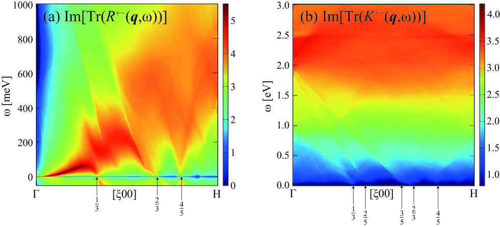
Figure 1: High-resolution calculation of ${\rm Im}[{\rm Tr}(R^{+-}(\omega))]$, together with ${\rm Im}[({\rm Tr}(K^{+-}(\omega))]$ for Fe in LDA by the method described in Ref.Okumura et al., 2019. Units in y-axis are in arbitrary logarithmic scales.

By definition of the extended Heisenberg model, we can reproduce Fig.1 by the linearization of the extended Heisenberg model. For ${\bf q}$ which is a little away from $\Gamma$, we have damping responses that can be well described by a simple equation of motion of spins such as the Landau-Lifshiz-Gilbert equation. At larger ${\bf q}$ (that is, at small ${\bf R}-{\bf R}^{\prime}$), we may need complicated friction mechanism. We see some resonances related to the hybridization of the Stone-excitation with SWs. The low energy excitations around the starting point of the Stoner-excitation boundaries at $\omega=0$ may have chances to generate some commensurate nonlinear motions of spins. In the case of Co and so on with two or more atoms in the cell, the optical branches of SWs do not necessarily exist because of the damping responses as shown in Fig.7 in Ref.Okumura et al., 2019. The degree of freedom of orbital-dependent spins may be important for generating frictions if the motions of spin magnetic moments are not described well by rigid spin rotations. The orbital-dependent Heisenberg parameter was analyzed in Ref.Kvashnin et al., 2016. We expect that the nonlinear motion of spins given by the extended Heisenberg model is quite useful in comparison with the conventional Heisenberg model.

To analyze all such nonlinear effects, we may perform semiquantum dynamics as was performed in Refs. Barker and Bauer, 2019; Barker et al., 2020 based on Eq.(3). We can determine even $T_{\rm c}$ by such a dynamics. Generally speaking, we can obtain the extended Heisenberg model just from any dynamical linear response function. It is possible to include spin-orbit coupling in the response $R^{+-}$. Furthermore, we can take into account higher-level electronic correlation effects as well as the phonon effect in the evaluation of $R^{+-}$. Then we will use the extended Heisenberg model as the basis for performing realistic simulations. Not only the fluctuations of spin magnetic moments but also those of the orbital magnetic moments might be taken into account along the line of the extended Heisenberg model.

III summary

We have introduced the extended Heisenberg model that is determined by the dynamical linear response. That is, we have the equation of motion of transverse spins with $J_{{\bf R}m{\bf R}^{\prime}m^{\prime}}(t-t^{\prime})$, which describes the orbital-dependent retarded exchange coupling.

We have discussed what types of physical mechanisms can be included in $J_{{\bf R}m{\bf R}^{\prime}m^{\prime}}(t-t^{\prime})$ on the basis of our high-resolution calculation of spin susceptibility for Fe in LDA. High-resolution calculations clearly reveal physical mechanisms that were missing in the low-resolution calculations. We see not only the damping of SWs, but also the hybridization between SWs and the Stoner excitations.

We believe that we should analyze spin dynamics on the basis of the extended Heisenberg model, which plays a key role in connecting first-principles calculations with realistic micro-magnetism simulations via atomistic spin dynamics. The extended Heisenberg model can be simplified to the Landau-Lifshiz-Gilbert equation. Such formulation should be useful for the theoretical analysis related to spintronics Mahmoud et al. (2020); Hula et al. (2021); Kainuma et al. (2021).