Stationary distributions of propelled particles as a system with quenched disorder

Abstract

This article is the exploration of the viewpoint within which propelled particles in a steady state are regarded as a system with quenched disorder. The analogy is exact when the rate of the drift orientation vanishes and the linear potential, representing the drift, becomes part of an external potential, resulting in the effective potential $u_{eff}$. The stationary distribution is then calculated as a disorder-averaged quantity by considering all contributing drift orientations. To extend this viewpoint to the case when a drift orientation evolves in time, we reformulate the relevant Fokker-Planck equation as a self-consistent relation. One interesting aspect of this formulation is that it is represented in terms of the Boltzmann factor $e^{-\beta u_{eff}}$. In the case of a run-and-tumble model, the formulation reveals an effective interaction between particles.

I Introduction

Within the two standard models of propelled motion, the run-and-tumble (RTP) and active Brownian particle (ABP) model, particles are subject to a drift of constant magnitude v0 but randomized orientation. The time evolution of the drift is what prevents a system from attaining an equilibrium. The evolution of the orientation in each model is governed by a different stochastic process. In the RTP model, the new direction is assigned sporadically at intervals drawn from Poisson distribution. A new orientation can take on any value with equal probability. In the ABP model, the orientation undergoes diffusion. The rate of orientation change in the RTP model is $\alpha$ and the angular diffusion in the ABP model is $D_{r}$.

Despite the apparent simplicity of an ideal-gas model of propelled particles, there is no available analytical solution for stationary distributions. One noted exception is the RTP model in one dimension with drift limited to two values, $v=\pm v_{0}$ Schnitzer93 ; Cates08 ; Cates09 ; Angelani17 ; Dhar18 ; Dhar19 ; Razin20 . Yet even a simple extension to three drifts $v=0,\pm v_{0}$ leads to considerable increase in complexity Basu20 . (The third model of propelled motion is the active Ornstein Uhlenbeck particles, AOUP Martin21a ; Martin21b ; however, in this work we exclusively focus on the RTP and ABP models.)

In this work, we take a different point of view to characterize stationary distributions of propelled particles. We start by considering a stationary state of propelled particles at exactly $\alpha=D_{r}=0$. Under these conditions, the unit vector ${\bf u}_{v}$, representing orientation of a drift, stops evolving in time and as a consequence the system attains equilibrium. The result is a mixture of particles with different drift orientations. And because the drift orientations are randomly distributed, the situation corresponds to a system with quenched disorder. The stationary distribution is a disorder-averaged distribution that takes into account all drift orientations.

The resulting distribution for the condition $\alpha=Dr=0$ represents the largest deviation from the distribution for the same system but for passive Brownian particles. Since in the limit $\alpha\to\infty$ and/or $D_{r}\to\infty$ the distribution converges to that of passive particles, this limit is generally regarded as representing an equilibrium. The suggestion, therefore, that the opposite limit $\alpha,D_{r}\to 0$ corresponds to an equilibrium appears to contradict this view. If we look into the entropy production $\Pi$ that is used as a quantification of distance from the equilibrium, we find that $\Pi$ vanishes as $\alpha,D_{r}\to 0$, supporting the claim that this limit represents an equilibrium. The opposite limit $\alpha\to\infty$ is found to yield the largest possible value of $\Pi$, indicating the largest deviations from equilibrium — a surprising result given that the distribution in that limit is the same as that for passive Brownian particles.

The central quantity that emerges in analyzing the limit $\alpha,D_{r}\to 0$, is the effective external potential, which is the original external potential $u_{ext}$ plus the linear potential representing a drift, $u_{eff}=u_{ext}+[{\bf u}_{v}\cdot{\bf r}]v_{0}/D$. One way to go beyond the decoupled limit, is to expand the stationary distribution perturbatively as $n\approx n_{0}+\alpha n_{1}$. This approach, however, leads to a rather complex expression for $n_{1}$ without offering valuable insights. Instead we reformulate the stationary Fokker-Planck equation (FP) as a self-consistent relation (SC). The central quantity of the SC formulation is the Boltzmann factor $e^{-\beta u_{eff}}$. Within the SC formulation, propelled particles appear as if they were coupled, but the effective attraction has the “chemical” origin and arises when particles of different drift orientations are regarded as different species that undergo a continuous conversion. The SC formulation is used as a basis for numerical computation of stationary distributions, an alternative procedure to dynamic simulations.

This work is organized as follows. In Sec. (II) we introduce a general FP equation of propelled particles for an arbitrary dimension $d$. In Sec. (III) we consider exact distributions for a decoupled condition $\alpha=D_{r}=0$, which represents the system with quenched disorder. In Sec. (IV) we develop the self-consistent framework for solving the stationary FP equation. The goal of such a framework is to gain insights as well as to look for alternative numerical schemes other than dynamic simulations. In Sec. (V) we analyze the entropy production of a two-state RTP model.

II Theoretical framework

The motion of an ideal-gas of propelled particles in a general $d$-dimensional space, with both RTP and ABP type of motion, is governed by the following Fokker-Planck equation (FP)

$$\frac{\partial n}{\partial t} = D\nabla^{2}n-v_{0}{\bf u}_{v}\cdot\mbox{\boldmath$\nabla$}n+\beta D\mbox{\boldmath$\nabla$}\cdot[n\mbox{\boldmath$\nabla$}u_{ext}]$$ (1)

$$- \alpha\bigg{[}n-\frac{1}{\Omega_{v}}\int d{\Omega}_{v}\,n\bigg{]}+D_{r}\hat{L}_{S}n,$$

where the distribution $n\equiv n({\bf r},{\bf u}_{v},t)$ is the function of the position ${\bf r}$, drift orientation ${\bf u}_{v}$ (${\bf u}_{v}$ is a unit vector), and time $t$, and is normalized to unity as $\int d{\bf r}\,n({\bf r},{\bf u}_{v},t)=1$. The first line in Eq. (1) governs the evolution of particle positions and involves standard diffusion, drift of constant magnitude $v_{0}$, and the interaction with external forces due to a conservative potential $u_{ext}({\bf r})$.

The second line in Eq. (1) governs the evolution of the unit vector ${\bf u}_{v}$ which determines the orientation of a drift. The time evolution of ${\bf u}_{v}$ is what prevents the system from attaining equilibrium. The first term gives rise to the RTP type of motion, where $\Omega_{v}=\int d{\Omega}_{v}$ is the area of a unit sphere in a given dimension. The RTP motion is represented as a "reaction" process where particles of different orientations are continuously created and destroyed yet their total number is conserved. The ABP motion is represented as a diffusion of a unit vector ${\bf u}_{v}$ on a surface of a sphere and the operator $\hat{L}_{S}$ is a spherical Laplacian operator on the $(d-1)$-sphere.

For the explicit dimension $d=2$ the second line in Eq. (1) becomes

$$\frac{\partial n}{\partial t}=-\mbox{\boldmath$\nabla$}\cdot{\bf j}-\alpha\bigg{[}n-\frac{1}{2\pi}\int_{0}^{2\pi}d\theta_{v}\,n\bigg{]}+D_{r}\frac{\partial^{2}n}{\partial\theta_{v}^{2}}.$$ (2)

where we introduce the flux

$${\bf j}({\bf r},{\bf u}_{v})=-D\mbox{\boldmath$\nabla$}n+v_{0}{\bf u}_{v}n-\beta D\mbox{\boldmath$\nabla$}\cdot[n\mbox{\boldmath$\nabla$}u_{ext}].$$

Because Eq. (1) and Eq. (2) involve creation-destruction of particles with different orientations, it is not immediately clear if the total number of particles is conserved. To demonstrate that this is the case, we integrate Eq. (2) over the space domain within which the system is confined,

$$\frac{\partial N}{\partial t}=-\alpha\bigg{[}N-\frac{1}{\Omega_{v}}\int d{\Omega}_{v}\,N\bigg{]}+D_{r}\frac{\partial^{2}N}{\partial\theta_{v}^{2}},$$ (3)

where we define the number of particles with particular orientation as $N({\bf u}_{v})=\int d{\bf r}\,n({\bf r},{\bf u}_{v})$. Note that $\int d{\bf r}\,\mbox{\boldmath$\nabla$}\cdot{\bf j}=0$ since particles do not enter or leave the prescribed domain. Finally, if we integrate Eq. (3) over all orientations and define $\bar{N}=\frac{1}{\Omega_{v}}\int d\Omega_{v}\,N({\bf u}_{v})$, we have

$$\frac{\partial\bar{N}}{\partial t}=-\alpha\big{[}\bar{N}-\bar{N}\big{]}+D_{r}\Big{[}\frac{\partial N}{\partial\theta_{v}}\Big{]}_{0}^{2\pi}=0,$$ (4)

where the second term cancels out as a result of periodic boundary conditions. The total number of particles, therefore, is conserved.

At this point, we introduce the "effective" external potential defined as

$$\beta u_{eff}=\beta u_{ext}-\frac{v_{0}}{D}[{\bf u}_{v}\cdot{\bf r}],$$ (5)

which is the external potential plus the linear potential for representing a drift. As we limit our analysis to stationary distributions, the time-independent FP equation of interest is

$$0=D\nabla^{2}n+\beta D\mbox{\boldmath$\nabla$}\cdot[n\mbox{\boldmath$\nabla$}u_{eff}]-\alpha\bigg{[}n-\frac{1}{\Omega_{v}}\int d{\Omega}_{v}\,n\bigg{]}+D_{r}\hat{L}_{S}n.$$ (6)

The stationary distribution that accounts for all orientations is defined as

$$\bar{n}({\bf r})=\frac{1}{\Omega_{v}}\int d{\Omega}_{v}\,n({\bf r},{\bf u}_{v}),$$

where the bar indicates the averaging procedure.

III Exact treatment in a decoupled limit, $\alpha=0$ and $D_{r}=0$

In this section we obtain distributions $n$ for a decoupled condition given by $\alpha=D_{r}=0$. Because under such circumstances ${\bf u}_{v}$ stops to evolve in time, the system is in equilibrium, but the distribution of drift orientations introduces quenched disorder.

By setting both $\alpha$ and $D_{r}$ to zero, Eq. (6) reduces to

$$0=D\nabla^{2}n_{0}+\beta D\mbox{\boldmath$\nabla$}\cdot[n_{0}\mbox{\boldmath$\nabla$}u_{eff}].$$ (7)

The result is the standard diffusion equation for a particle in the external potential $u_{eff}$. The solution is proportional to the Boltzmann weight

$$n_{0}({\bf r},{\bf u}_{v})\propto e^{-\beta u_{ext}}e^{[{\bf u}_{v}\cdot{\bf r}]v_{0}/D}.$$

The subscript "0" is used to indicate that the solution is true only for the case $\alpha=D_{r}=0$. The actual stationary distribution is obtained by averaging over all possible drifts ${\bf u}_{v}$ uniformly distributed over all orientations and given by

$$\bar{n}_{0}({\bf r})\propto\int d\Omega_{v}\,e^{-\beta u_{ext}+[{\bf r}\cdot{\bf u}_{v}]v_{0}/D}.$$ (8)

Quenched disorder is the inherent feature of the system in the decoupled limit.

If $u_{ext}$ depends on particle positions only, then the Boltzmann factor can be separated and above equation can be written as

$$\bar{n}_{0}({\bf r})\propto e^{-\beta u_{ext}({\bf r})}\int d\Omega_{v}\,e^{[{\bf r}\cdot{\bf u}_{v}]v_{0}/D}.$$

All orientations in the above formulation are equally likely and there is no bias for any particular direction. But if the external potential contributes to particle orientations, $u_{ext}\equiv u_{ext}({\bf r},{\bf u}_{v})$, a case that might arise for particles with dipole moment, the orientation would no longer be distributed uniformly and we would have

$$\bar{n}_{0}({\bf r})\propto\int d\Omega_{v}\,e^{-\beta u_{ext}({\bf r},{\bf u}_{v})}e^{[{\bf r}\cdot{\bf u}_{v}]v_{0}/D}.$$

Such orientation bias would reduce quenched disorder. In this work, however, we limit our interest to the position dependent potentials.

III.1 harmonic trap

We next consider a number of specific potentials. For a harmonic potential $\beta u_{ext}=\frac{1}{2}Kr^{2}$, $u_{eff}=\frac{1}{2}Kr^{2}-[{\bf u}_{v}\cdot{\bf r}]v_{0}/D$ and the Boltzmann distribution representing the decoupled limit is

$$n_{0}({\bf r},{\bf u}_{v})\propto e^{-\frac{1}{2}\beta Kr^{2}}e^{[{\bf u}_{v}\cdot{\bf r}]v_{0}/D}.$$ (9)

The disorder averaged distribution is obtained using Eq. (8). For dimension $d=2$ we have $d\Omega_{v}=d\theta_{v}$, leading to

$$\bar{n}_{0}(r)\propto e^{-\frac{1}{2}\beta Kr^{2}}\int_{0}^{2\pi}d\theta_{v}\,e^{r\cos\theta_{v}v_{0}/D}.$$

After evaluating the integral we find

$$\bar{n}_{0}(r)=\bigg{[}\bigg{(}\frac{\beta K}{2\pi}\bigg{)}e^{-\frac{1}{2}\beta Kr^{2}}\bigg{]}\bigg{[}e^{-\frac{v_{0}^{2}}{2D^{2}\beta K}}I_{0}\left(\frac{v_{0}r}{D}\right)\bigg{]}.$$ (10)

The two terms in square-brackets indicate different contributions. The first is the usual Gaussian distribution for passive particles in a harmonic potential. The second term, represented by the modified Bessel function $I_{0}(x)$, is the contribution due to propelled motion. This term diverges far away from the center of the trap as $I_{0}(x)\approx e^{x}/\sqrt{2\pi x}$ and gives rise to particle deposition at the border of a trap rudi18 .

For dimension $d=3$, the drift orientation is uniformly distributed on a unit sphere with $d\Omega_{v}=\sin\theta_{v}d\theta_{v}d\phi_{v}$. The disorder averaged distribution obtained using Eq. (8) is

$$\bar{n}_{0}(r)\propto e^{-\frac{1}{2}\beta Kr^{2}}\int_{0}^{2\pi}d\phi_{v}\int_{0}^{\pi}d\theta_{v}\,\sin\theta_{v}\,e^{r\cos\theta_{v}v_{0}/D},$$

and evaluates to

$$\bar{n}_{0}(r)=\bigg{[}\bigg{(}\frac{\beta K}{2\pi}\bigg{)}^{3/2}\ e^{-\frac{1}{2}\beta Kr^{2}}\bigg{]}\bigg{[}e^{-\frac{v_{0}^{2}}{2D^{2}\beta K}}\frac{D}{v_{0}r}\sinh\left(\frac{v_{0}r}{D}\right)\bigg{]}.$$ (11)

The result is similar to that in Eq. (10). The deposition of particles predicted by (10) and (11) correspond to the optimal deposition. Any finite value of $\alpha>0$ or $D_{r}>0$ would make this deposition less extreme. To see how the true stationary distributions $\bar{n}(r)$ evolve toward $\bar{n}_{0}(r)$ as $\alpha$ or $D_{r}$ tend to zero, in Fig. (1) we plot the distributions obtained from dynamic simulations for both the RTP and ABP type of motion for particles trapped in the harmonic potential and for the dimension $d=2$. The results are compared to the limiting functional form in Eq. (10).

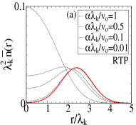
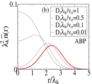
Figure 1: Distributions of propelled particles in the potential $u_{ext}={Kr^{2}}/{2}$ obtained from dynamic simulations for $d=2$ (dashed black lines). $\lambda_{k}=\sqrt{{2}/{\beta K}}$ is the trap size and the results are for $v_{0}\lambda_{k}/D=5$. The solid red line corresponds to the expression in (10). The results in (a) are for RTP and those in (b) for ABP type of motion.

III.2 particles in a confinement with 1D geometry

If a confining potential has 1D geometry, the system is effectively one-dimensional. The simplest example is for particles trapped between two parallel walls. Since $u_{ext}=0$, the effective potential is

$$\beta u_{eff}(x)=-\frac{v_{x}x}{D},$$

where $x$-axis is perpendicular to the walls.

The normalized Boltzmann distribution for this effective potential, representing the decoupled limit, is

$$n_{0}(x,v_{x})=\frac{1}{2h}\frac{v_{x}h}{D}\frac{e^{\frac{v_{x}x}{D}}}{\sinh(\frac{v_{x}h}{D})}.$$ (12)

For the dimension $d=2$ the disorder averaged distribution is given by

$$\bar{n}_{0}(x)=\frac{1}{2\pi}\int_{0}^{2\pi}d\theta_{v}\,n_{0}(x,v_{0}\cos\theta_{v}).$$ (13)

Using $\frac{d\cos\theta_{v}}{d\theta_{v}}=-\sin\theta_{v}$ and $v_{x}=v_{0}\cos\theta_{v}$, we obtain

$$d\theta_{v}=-\frac{dv_{x}}{\sqrt{v_{0}^{2}-v_{x}^{2}}},$$

and the integral in Eq. (12) can be rewritten as

$$\bar{n}_{0}(x)=\frac{1}{\pi}\int_{-v_{0}}^{v_{0}}dv_{x}\,\frac{n_{0}(x,v_{x})}{\sqrt{v_{0}^{2}-v_{x}^{2}}}.$$ (14)

Or more generally, we can write

$$\bar{n}_{0}(x)=\int_{-v_{0}}^{v_{0}}dv\,P(v)n_{0}(x,v),$$ (15)

where we use $v\equiv v_{x}$ and for $d=2$ the distribution of drifts is

$$P(v)=\frac{1}{\pi}\frac{1}{\sqrt{v_{0}^{2}-v^{2}}}.$$ (16)

Even if the drift orientations are uniformly distributed in the variable $\theta_{v}$, when considering the variable $v_{x}$, there is a considerable inhomogeneity with peaks at $v=\pm v_{0}$.

For the dimension $d=3$ the disorder averaged distribution is given by

$$\bar{n}_{0}(x)=\frac{1}{4\pi}\int_{0}^{\pi}d\theta_{v}\int_{0}^{2\pi}d\phi_{v}\,\sin\theta_{v}\,n_{0}(x,v_{0}\cos\theta_{v}),$$ (17)

and evaluates to (see Appendix A for the derivation)

$$\bar{n}_{0}(x)=\frac{1}{2v_{0}}\int_{-v_{0}}^{v_{0}}dv\,n_{0}(x,v).$$

Comparing to Eq. (15), this implies that $P(v)$ is uniform on the interval $-v_{0}\leq v\leq v_{0}$,

$$P(v)=\frac{1}{2v_{0}}.$$ (18)

The expressions in (16) and (18) show strong dependence of $P(v)$ on the system dimensionality and suggest that the particle deposition at the walls is larger for $d=2$ than that for $d=3$.

The next question is, can the integral in (15) be evaluated exactly. Even for uniform distribution $P(v)$, representing the system in $d=3$, resulting analytical expression is rather complex. It involves Hurwitz-Lerch zeta and hypergeometric functions. From practical point of view, it is more convenient to evaluate Eq. (15) numerically for both $d=2$ and $d=3$.

In Fig. (2) we show an analogous plot to that in (1) but for particles between two parallel walls and decreasing values of $\alpha$ and $D_{r}$ in order to demonstrate convergence of the distributions to $\bar{n}_{0}$. The distribution $\bar{n}_{0}$ correctly delimits the range within which the distributions $n$ evolve.

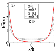
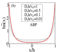
Figure 2: Distributions of propelled particles between two parallel walls separated by $2h$ obtained from dynamic simulations for $d=2$ (dashed black lines). The results are for $v_{0}h/D=10$. The solid red line corresponds to the distribution $\bar{n}_{0}(x)$ in the quenched disorder limit. The results in (a) are for RTP motion and (b) for ABP motion.

A different example of a potential with 1D geometry is the harmonic potential $u_{ext}=\frac{Kx^{2}}{2}$. The normalized Boltzmann distribution corresponding to the decoupled limit in this case is

$$n_{0}(x,v)=\sqrt{\frac{\beta K}{2\pi}}e^{-v^{2}/2\beta KD^{2}}e^{\frac{vx}{D}-\frac{\beta Kx^{2}}{2}},$$

and the disorder averaged distribution is obtained from Eq. (15) for an appropriate $P(v)$. For $d=2$ the integral must be evaluated numerically, and for $d=3$ it evaluates to the following expression

$$\bar{n}_{0}(x)=\frac{D}{2v_{0}\lambda_{k}^{2}}\bigg{(}\text{erf}\bigg{[}\frac{x}{\lambda_{k}}+\frac{1}{2}\frac{v_{0}\lambda_{k}}{D}\bigg{]}-\text{erf}\bigg{[}\frac{x}{\lambda_{k}}-\frac{1}{2}\frac{v_{0}\lambda_{k}}{D}\bigg{]}\bigg{)},$$ (19)

where $\text{erf}(x)$ is the error function and $\lambda_{k}=\sqrt{2/\beta K}$. Unlike the results in (10) and (11), the simple separation between the passive and propelled motion is not possible.

In Fig. (3) we plot the distributions $\bar{n}(x)$ for the potential $u_{ext}=\frac{Kx^{2}}{2}$ for $d=2$ for decreasing values of $\alpha$ and $D_{r}$, in analogy to figures in (1) and (2). Once again, the distributions $\bar{n}_{0}$ correctly delimit the range within which the true distributions for finite $\alpha$ or $D_{r}$ can be found.

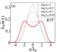
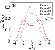
Figure 3: Distributions of propelled particles in the external potential $u_{ext}={Kx^{2}}/{2}$ obtained from dynamic simulations for $d=2$ (dashed black lines). $\lambda_{k}=\sqrt{{2}/{\beta K}}$ is the trap size and the results are for $v_{0}\lambda_{k}/D=5$. The solid red line corresponds to the distribution $\bar{n}_{0}(x)$. The results in (a) are for RTP and (b) for ABP motion.

Earlier we briefly discussed the dependence of $P(v)$ on dimensionality when comparing $P(v)$ for $d=2$ and $d=3$ in (16) and (18) and the implication of those differences on the accumulation of particles at the trap borders. Below we provide a general expression of $P(v)$, derived in Appendix A, for a general dimension $d>1$,

$$P(v)=\frac{1}{v_{0}\sqrt{\pi}}\frac{\Gamma[d/2]}{\Gamma[(d-1)/2]}\bigg{(}1-\frac{v^{2}}{v_{0}^{2}}\bigg{)}^{(d-3)/2},~{}~{}\text{if}~{}~{}d>1,$$ (20)

with $P(v)$ normalized and defined on the interval $-v_{0}\leq v\leq v_{0}$. For $d=1$ the distribution is represented in terms of delta functions as drifts in this dimension are limited to two values $v=\pm v_{0}$ Razin20 ,

$$P(v)=\frac{1}{2}\big{[}\delta(v+v_{0})+\delta(v-v_{0})\big{]},~{}~{}\text{if}~{}~{}d=1$$ (21)

Clearly, the distribution $\bar{n}_{0}$ calculated using (15) depends on $P(v)$. For large $d$ the distribution $P(v)$ approaches a Gaussian functional form

$$P(v)\approx\sqrt{\frac{d}{2\pi v_{0}^{2}}}e^{-\frac{d}{2}(v/v_{0})^{2}},$$

and in the limit $d\to\infty$, $P(v)\to\delta(v)$, and the system loses its quenched disorder — all particles have zero drift and the system becomes identical with that for passive Brownian particles.

In Fig. (4) we plot the distributions $\bar{n}_{0}(x)$ for two different external traps, $u_{ext}=\frac{Kx^{2}}{2}$ and for confinement between two walls, for $P(v)$ in (20) and (21) corresponding to different $d$. The plots demonstrate strong dependence on $d$, in particular, it shows increased deposition of particles around the trap borders as dimensionality goes down.

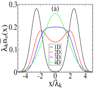
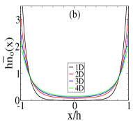
Figure 4: Distributions $\bar{n}_{0}(x)$ for an external potential (a) $u_{ext}=Kx^{2}/2$ and (b) for particles between two walls, for different system dimensionality $d$. The distributions are for $v_{0}\lambda_{k}/D=5$ and $v_{0}h/D=10$.

A similar dimensionality dependence is found in the opposite limit of large $\alpha$ and/or $D_{r}$, accurately represented by the concept of effective temperature Kardar15 ; Kurchan13 ; Szamel14 valid for $d>1$,

$$\frac{T_{\rm eff}}{T}=1+\frac{1}{d(d-1)}\frac{v^{2}_{0}}{D(\alpha+D_{r})},$$ (22)

where increased dimensionality $d$ brings $T_{eff}$ closer to thermodynamic temperature $T$. In the limit $d\to\infty$, $T_{eff}=T$. The reason for this behavior is rather simple. The constant velocity $v_{0}$ and the associated kinetic energy is distributed into $d$ components. For increased dimensionality, the extra kinetic energy that goes to each degree of freedom is reduced, giving rise to the observed cooling effect.

IV Self-consistent formulation

The next step is to try to expand the distribution $n$ around the decoupled limit as $n\approx n_{0}+\alpha n_{1}$. However, such a systematic expansion yields expressions which are complex and not very insightful. Instead, we reformulate the stationary FP equation as a self-consistent relation (SC). The resulting formulation yields interesting insights, provides basis for an alternative computation of distributions, and can be used for obtaining perturbative expansion of $n$.

IV.1 RTP particles

To keep things simple, we consider a system with 1D geometry. For the RTP motion the stationary FP equation in 1D can be written as

$$0=Dn^{\prime\prime}+\beta D\big{[}u_{eff}^{\prime}n\big{]}^{\prime}+\alpha(\bar{n}-n),$$

where the effective potential incorporates the drift as $\beta u_{eff}=\beta u_{ext}-\frac{v}{D}x,$ and the disorder averaged distribution is $\bar{n}=\int dv\,P(v)n(n,x)$. The same equation can be written as

$$0=n^{\prime\prime}+\beta\big{[}u_{eff}^{\prime}n\big{]}^{\prime}+s$$ (23)

where

$$s=\frac{\alpha}{D}(\bar{n}-n)$$ (24)

plays the role of the source function. Note that the source function satisfies $\int dx\,s(x,v)=0$ and $\int dv\,P(v)s(x,v)=0$.

By introducing the source function, Eq. (6) can be regarded as an inhomogeneous second-order differential equation. The solution then can be obtained using the method of variation of parameters. To proceed, we first need solutions for the homogenous equation. The two possible solutions are

$$y_{0}=e^{-\beta u_{eff}},~{}~{}~{}~{}y_{1}=y_{0}Y_{0},$$ (25)

where

$$Y_{0}=\int dx\,e^{\beta u_{eff}}.$$ (26)

The first solution corresponds to the Boltzmann distribution. The second solution is normally rejected on physical grounds due to its non-vanishing local flux, $D\rho^{\prime}+u_{eff}^{\prime}\rho\neq 0$, when dealing with passive particles. As we will see, this solution becomes relevant for describing propelled particles.

The solution of the second order inhomogeneous equation can be expressed as

$$n=Ay_{0}+By_{1}+\bigg{[}y_{0}\int dx\,\frac{y_{1}}{w}s-y_{1}\int dx\,\frac{y_{0}}{w}s\bigg{]},$$ (27)

where $A$ and $B$ are undefined coefficients and $w=y_{0}y_{1}^{\prime}-y_{0}^{\prime}y_{1}$ is the Wronskian that for the present case evaluates as $w=y_{0}$. The first two terms constitute a complementary solution and the last term is the particular solution. Since the second term does not produce a vanishing flux, $B$ is set to zero. After using (25) and substituting (24) for the source function, the solution transforms into the desired SC relation

$$n=Ae^{-\beta u_{eff}}+\frac{\alpha e^{-\beta u_{eff}}}{D}\bigg{[}\int dx\,(\bar{n}-n)Y_{0}-Y_{0}\int dx\,(\bar{n}-n)\bigg{]},$$ (28)

where $A$ is determined from the condition of normalization $\int_{L}dx\,n(x,v)=1$ on the domain $L$ prescribed by a physical problem. Note that for $\alpha=0$, we recover $n=n_{0}$.

The SC relation in (28) reveals a certain mean-field character of the formulation Frydel16 and the presence of the effective interactions between particles — particles appear to be "attracted" toward the average distribution $\bar{n}$. The origin of this coupling between particles, however, is different from that in a system of truly interacting particles. It is caused by the "reaction" part of the FP equation, as particles of different drift, regarded as belonging to different species, exchange their identity.

If the RTP particles are confined between two parallel walls then $\beta u_{eff}=-\frac{vx}{D},$ and

$$Y_{0}=-\frac{D}{v}e^{-\frac{vx}{D}},$$

and the SC relation becomes

$$n=An_{0}+\alpha\int_{-h}^{x}dx^{\prime}\,\bigg{[}\frac{1-e^{\frac{v}{D}(x-x^{\prime})}}{v}\bigg{]}(\bar{n}-n).$$ (29)

The above SC relation is next used as a basis for numerical computation of the distributions $n$ based on iterative procedure starting with $n_{0}$. For $\alpha\geq 0.5$ a mixing parameter is used, $0<\gamma<1$, for generating the next distribution as $n_{new}\equiv(1-\gamma)n_{old}+\gamma n_{new}$. For the bin size $\Delta x=0.01$ the convergence is attained within ten to twenty iterations (amounting to a few seconds of the CPU time, a significant improvement over dynamic simulations).

Fig. (5) plots the numerically calculated stationary distributions for $d=2$ (using the distribution $P(v)$ in (16)). The distributions are in perfect correspondence with those obtained from dynamic simulations.

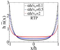
Figure 5: Distributions $\bar{n}(x)$ obtained numerically using the SC formulation of the FP equation for the RTP particles between two walls for $d=2$ and $v_{0}h/D=10$. Circles correspond to simulation data points.

The SC formulation in (28), or that for particles between walls in (29), can also be used for constructing subsequent terms within the perturbative approach, $n=n_{0}+\alpha n_{1}+\dots$, by inserting $n_{0}$ on the right hand side of those equations. If considering Eq. (29), we get

$$n_{1}=\int_{-h}^{x}dx^{\prime}\,\bigg{[}\frac{1-e^{\frac{v}{D}(x-x^{\prime})}}{v}\bigg{]}(\bar{n}_{0}-n_{0})+Cn_{0},$$ (30)

where the constant $C$ is such as to ensure the condition $\int_{-h}^{h}dx\,n_{1}(x,v)=0$, since the perturbation $n_{1}$ cannot create or destroy particles, only redistribute them in the interval $-h\leq x\leq h$. We recall that $n_{0}(x,v)$ for the system between walls is given in Eq. (13), however, inserting this expression into (30) does not lead to analytical results and the perturbative formulation itself does not shed any additional light.

We next consider a harmonic potential, in which case $\beta u_{eff}=-\frac{vx}{D}+\frac{\beta Kx^{2}}{2},$

$$Y_{0}=\frac{\lambda_{k}\sqrt{\pi}}{2}e^{-(\frac{v\lambda_{k}}{2D})^{2}}\text{erfi}\Big{[}\frac{x}{\lambda_{k}}-\frac{1}{2}\frac{v\lambda_{k}}{D}\Big{]},$$

where $\text{erfi}(x)=-i\text{erf}(ix)$ is the imaginary error function, and the SC equation expressed in terms of definite integrals is

$$ne^{\beta u_{eff}}=A+\frac{\alpha}{D}\bigg{[}\int_{-\infty}^{x}dx^{\prime}\,(\bar{n}-n)Y_{0}-Y_{0}\int_{-\infty}^{x}dx^{\prime}\,(\bar{n}-n)\bigg{]}.$$ (31)

For numerical integration the limits $x=\pm\infty$ are substituted by $x=\pm x_{c}$ where the cutoff distance $x_{c}$ is large enough so that $n(\pm x_{c},v)\approx 0$. Numerically calculated distributions for $d=2$ are shown in Fig. (6).

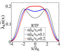
Figure 6: Distributions $\bar{n}(x)$ obtained numerically using the SC formulation for the RTP particles in the potential $u_{ext}=Kx^{2}/2$ for $d=2$ and $v_{0}\lambda_{k}/D=5$. Circles correspond to simulation data points.

Again, the distributions are in perfect correspondence with those obtained from dynamic simulations.

IV.2 ABP particles

Self-consistent relation could similarly be established for the ABP type of motion. Considering the system dimension $d=2$ and a system with 1D geometry, the stationary FP equation that describes this situation, obtained using Eq. (2) with $\alpha=0$ but for finite $D_{r}$, is

$$0=n^{\prime\prime}+\beta D\big{[}u_{eff}^{\prime}n\big{]}^{\prime}+\frac{D_{r}}{D}\frac{\partial^{2}n}{\partial\theta_{v}^{2}},$$ (32)

where $n\equiv n(x,\theta_{v})$. If the source term is defined as

$$s=\frac{D_{r}}{D}\frac{\partial^{2}n}{\partial\theta_{v}^{2}},$$

we arrive at a similar form to that in (23), and can follow up with the same procedure. In the case of ABP motion, the expressions are more economic if the distributions are defined in terms of $\theta_{v}$ rather than $v\equiv v_{x}$.

The SC relation that follows is

$$n=Ae^{-\beta u_{eff}}+\frac{D_{r}e^{-\beta u_{eff}}}{D}\bigg{[}\int dx\,Y_{0}\,\frac{\partial^{2}n}{\partial\theta_{v}^{2}}-Y_{0}\int dx\,\frac{\partial^{2}n}{\partial\theta_{v}^{2}}\bigg{]},$$ (33)

and can next be used as a basis for calculating stationary distributions. The results are shown in Fig. (7). Unlike for the RTP particles, the numerical method is less robust and larger number of iteration is required to reach convergence.

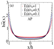
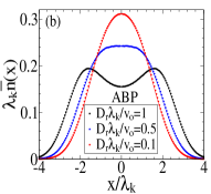
Figure 7: Distributions $\bar{n}(x)$ obtained numerically from the SC formulation for the ABP particles for $d=2$ (a) between two walls with $v_{0}h/D=10$ and (b) in the harmonic potential with $v_{0}\lambda_{k}/D=5$. Circles correspond to simulation data points.

V What is the true equilibrium?

There is an interesting consequence of treating the system with $\alpha=D_{r}=0$ as a reference point and considering deviations from it as a "distance" from equilibrium. According to this viewpoint, the system at $\alpha\to\infty$ or $D_{r}\to\infty$, represents the largest deviation — the conclusion that runs counter to more conventional point of view that regards as a reference state (and equilibrium) the limit $\alpha\to\infty$ or $D_{r}\to\infty$.

One way to resolve this controversy, of which reference point corresponds to equilibrium, is to resort to the arbitration of the entropy production, considered as a sophisticated way of quantifying the degree of violation of detailed-balance condition. We will not make calculations for the entropy production for our system. Instead we use the exact expression for the RTP s ystem in $d=1$, where $P(v)=\frac{1}{2}[\delta(v-v_{0})+\delta(v+v_{0})]$, found in Ref. Razin20 in Eq. (17) and given by

$$\Pi=\alpha\frac{hk\cosh hk-\sinh hk}{\frac{\alpha D}{v_{0}^{2}}hk\cosh hk+\sinh hk},$$ (34)

where $k=\frac{v_{0}}{D}\sqrt{1+\frac{\alpha D}{v_{0}^{2}}}$. In true equilibrium, $\Pi=0$. The larger the value of $\Pi$, we larger the deviation from equilibrium. If we plot $\Pi$ as a function of $\alpha$ for fixed $D$ and $v_{0}$ we discover that $\Pi(\alpha=0)=0$ and as $\alpha$ increases $\Pi$ grows monotonically and in the limit $\alpha\to\infty$ we have $\Pi(\alpha\to\infty)=\frac{v_{0}^{2}}{D}$. Such result appears to vindicate our viewpoint that the "correct" equilibrium corresponds to the decoupled limit, not the other way around. The reason for this surprising result is that even if the distribution $n$ becomes flat and the transport due to diffusion vanishes, a convective type of motion is still there.

VI Conclusion

This work starts by recognizing that at the precise condition $\alpha=D_{r}=0$, where orientation of the drifts becomes fixed and time independent, the system attains an equilibrium with quenched disorder. This intuitive interpretation permits us to obtain exact stationary distributions of propelled particles in confining potentials. The central quantity that emerges is the effective potential $u_{eff}$, which is the sum of an external potential and a linear potential for representing drift, and the Boltzmann factor $e^{-\beta u_{eff}}$.

In the second part of this work we construct the theoretical framework in which the decoupled state figures naturally. This is done by reformulating the stationary FP equation as a self-consistent relation, formulated in terms of the Boltzmann factor $e^{-\beta u_{eff}}$. The formulation reveals the presence of coupling between propelled particles (even if there are no true interactions between particles) as a result of "chemical" process, whereby particles with different drift are represented as different species that continuously exchange identities. The self-consistent formulation is used as a basis for numerical computation of stationary distributions, as an alternative to dynamic simulations. The SC formulation can also be used to expand $n$ perturbatively around $n_{0}$.

The viewpoint that considers the decoupled condition as an equilibrium state raises the question, so what the real equilibrium is? Generally, this privileged status is attributed to the limit $\alpha\to\infty$ and/or $D_{r}\to\infty$, since the distribution in those limits converges to that of passive Brownian particles. However, if we look into the entropy production $\Pi$ that is supposed to measure a distance from an equilibrium, we get the results that support the case for the decoupled limit as a true equilibrium.

The viewpoint that considers the decoupled condition as an equilibrium state raises the question, So what is the real equilibrium? Generally, equilibrium is attributed to the limit $\alpha\to\infty$ and/or $D_{r}\to\infty$, since the distribution in those limits converges to that of passive Brownian particles. However, if we look into the entropy production $\Pi$ that is supposed to measure a distance from equilibrium, we get the results that support the case for the decoupled limit as a true equilibrium.

VII DATA AVAILABILITY

The data that support the findings of this study are available from the corresponding author upon reasonable request.

Appendix A Distributions $P(v)$ for a general $d$-dimension

A general, disorder averaged distribution over drift orientations uniformly distributed on the surface of a unit sphere in $d$-dimension for the system with 1D geometry, such a system between two parallel walls or in the harmonic potential $u_{ext}=\frac{Kx^{2}}{2}$, is

$$\bar{n}_{0}(x)\propto\int_{0}^{2\pi}d\Omega_{v}\,n_{0}(x,v_{0}\cos\theta_{v}),$$

where $v_{x}=v_{0}\cos\theta_{v}$ is the velocity component in the direction perpendicular to the boundaries of a trap. The stationary distribution is uniform in the remaining directions.

Since for an arbitrary dimension $d$, $d\Omega$ is defined as

$$d\Omega=\sin^{d-2}\varphi_{1}\sin^{d-3}\varphi_{2}\cdots\sin d\varphi_{d-2}\,d\varphi_{1}\,d\varphi_{2}\cdots d\varphi_{d-1},$$

where $\theta=\varphi_{1}$, we may write

$$\int d\Omega_{v}\,n_{0}(x,v_{0}\cos\theta_{v})\propto\int_{0}^{\pi}d\theta_{v}\,\sin^{d-2}\theta_{v}\,\,n_{0}(x,v_{0}\cos\theta_{v}),$$

as the angles $\varphi_{k}$ for $k>1$ can be ignored. The above integral is transformed using $d\theta_{v}=-\frac{1}{v_{0}}\frac{dv}{\sin\theta_{v}},$ where $v\equiv v_{0}\cos\theta_{v}$, and $\sin\theta_{v}=\sqrt{1-\cos^{2}\theta_{v}}$ into

$$\int d\Omega_{v}\,n_{0}(x,v_{0}\cos\theta_{v})\propto\int_{-v_{0}}^{v_{0}}dv\,\bigg{(}1-\frac{v^{2}}{v_{0}^{2}}\bigg{)}^{\frac{d-3}{2}}\,n_{0}(x,v),$$

and the normalized distribution $P(v)$ for an arbitrary dimension $d$ is

$$P(v)=\frac{1}{v_{0}\sqrt{\pi}}\frac{\Gamma[\frac{d}{2}]}{\Gamma[\frac{d-1}{2}]}\bigg{(}1-\frac{v^{2}}{v_{0}^{2}}\bigg{)}^{\frac{d-3}{2}}.$$ (35)

References

- (1) M. J. Schnitzer, Theory of continuum random walks and application to chemotaxis, Phys. Rev. E 48, 2553 (1993).
- (2) J. Tailleur and M. E. Cates, Statistical Mechanics of Interacting Run-and-Tumble Bacteria, Phys. Rev. Lett. 100, 218103 (2008).
- (3) J. Tailleur and M. E. Cates, Sedimentation, trapping, and rectification of dilute bacteria, Europhys. Lett. 86, 60002 (2009).
- (4) L. Angelani, Confined run-and-tumble swimmers in one dimension, J. Phys. A: Math. Theor. 50, 325601 (2017).
- (5) K. Malakar, V. Jemseena, A. Kundu, K. V. Kumar, S. Sabhapandit, S. N. Majumdar, S. Redner, and A. Dhar, Steady state, relaxation and first-passage properties of a run-and-tumble particle in one-dimension, J. Stat. Mech.: Theory Exp. 043215 (2018).
- (6) A. Dhar, A. Kundu, S. N. Majumdar, S. Sabhapandit, and G. Schehr Run-and-tumble particle in one-dimensional confining potentials: Steady-state, relaxation, and first-passage properties Phys. Rev. E 99, 032132 (2019).
- (7) N. Razin, Entropy production of an active particle in a box, Phys. Rev. E (R) 102, 030103(R) (2020).
- (8) U. Basu, S.N. Majumdar, A. Rosso, S. Sabhapandit and G. Schehr, Exact stationary state of a run-and-tumble particle with three internal states in a harmonic trap, J. Phys. A: Math. Theor. 23, (2020).
- (9) D. Martin, J. O’Byrne, M. E. Cates, É. Fodor, C. Nardini, J. Tailleur, and F. van Wijland Statistical mechanics of active Ornstein-Uhlenbeck particles, Phys. Rev. E 103, 032607 (2021).
- (10) D. Martin, T. A. de Pirey, https://arxiv.org/abs/2009.13476.
- (11) A. P. Solon, Y. Fily, A. Baskaran, M. E. Cates, Y. Kafri, M. Kardar, and J. Tailleur, Pressure is not a state function for generic active fluids, Nature Physics 11, 673 (2015).
- (12) D. Frydel and R. Podgornik, Mean-field theory of active electrolytes: Dynamic adsorption and overscreening, Phys. Rev. E 97, 052609 (2018).
- (13) L. Berthier and J. Kurchan Non-equilibrium glass transitions in driven and active matter, Nat. Phys. 9, 310 (2013).
- (14) G. Szamel, Self-propelled particle in an external potential: Existence of an effective temperature, Phys. Rev. E 90, 012111 (2014).
- (15) D. Frydel, Mean Field Electrostatics Beyond the Point Charge Description, Adv. Chem. Phys. 160, 209 (2016).