Approximate inversion of discrete Fourier integral operators

Abstract

This paper introduces a factorization for the inverse of discrete Fourier integral operators that can be applied in quasi-linear time. The factorization starts by approximating the operator with the butterfly factorization. Next, a hierarchical matrix representation is constructed for the hermitian matrix arising from composing the Fourier integral operator with its adjoint. This representation is inverted efficiently with a new algorithm based on the hierarchical interpolative factorization. By combining these two factorizations, an approximate inverse factorization for the Fourier integral operator is obtained as a product of $O(\log N)$ sparse matrices of size $N\times N$. The resulting approximate inverse factorization can be used as a direct solver or as a preconditioner. Numerical examples on 1D and 2D Fourier integral operators, including a generalized Radon transform, demonstrate the performance of this new approach.

Keywords: Fourier integral operator; Radon transform; hierarchical matrices; hierarchical interpolative factorization; butterfly algorithm

AMS subject classifications: 35S30; 44A12; 65F05

1 Introduction

In this paper, we consider Fourier integral operators (FIOs) of the form

$$(\mathcal{L}f)(x)=\int_{\mathbb{R}^{d}}a(x,\xi)e^{2\pi i\Phi(x,\xi)}\hat{f}(\xi)\text{d}\xi.$$ (1.1)

Here, $\xi$ is the frequency variable, $x$ the spatial variable, $a(x,\xi)$ is a smooth amplitude function in both $x$ and $\xi$, $\Phi(x,\xi)$ is a smooth phase function in $(x,\xi)$ for $\xi\neq 0$ with the homogeneity relation $\Phi(x,\lambda\xi)=\lambda\Phi(x,\xi)$ for $\lambda$ positive, and $\hat{f}$ is the Fourier transform of $f$ defined by

$$\hat{f}(\xi)=\int_{\mathbb{R}^{d}}e^{-2\pi ix\cdot\xi}f(x)\text{d}x.$$ (1.2)

Typical uses of FIOs include the study of hyperbolic equations or integration over certain curved manifolds used in inverse problems. For instance, FIOs are commonly used to represent the solution to wave equations in $\mathbb{R}^{d}$ [12].

To introduce the discrete analog of an FIO in the $d$-dimensional case, we start with two Cartesian grids

$$X=\left\{x=\left(\frac{n_{1}}{n},\ldots,\frac{n_{d}}{n}\right),0\leq n_{1},\ldots,n_{d}<n\text{ and }n_{1},\ldots n_{d}\in\mathbb{Z}\right\},$$ (1.3)

$$\Omega=\left\{\xi=(n_{1},\ldots,n_{d}),-n/2\leq n_{1},\ldots,n_{d}<n/2\text{ with }n_{1},\ldots,n_{d}\in\mathbb{Z}\right\},$$ (1.4)

where the number of discretization points per dimension $n$ is assumed to be even for simplicity. The $d$-dimensional discrete Fourier integral operator of a function $f(x)$ is then defined by

$$(\mathcal{L}f)(x)\equiv(\mathcal{K}\hat{f})(x)=\sum_{\xi\in\Omega}a(x,\xi)e^{2\pi i\Phi(x,\xi)}\hat{f}(\xi)$$ (1.5)

for every $x\in\mathcal{X}$, where $\hat{f}$ is the discrete Fourier transform of $f$ defined by

$$\hat{f}(\xi)=\frac{1}{n^{d}}\sum_{x\in X}e^{-2\pi ix\cdot\xi}f(x).$$ (1.6)

The discrete FIO from (1.5) can be written in matrix form as

$$u={K}\hat{f}$$ (1.7)

with $\hat{f}=Ff$ and $u$ being the discrete Fourier transform and the discrete Fourier integral transform of $f$, respectively, evaluated at each discretization point. Notice that ${K}$ is a dense matrix of size $n^{d}\times n^{d}$, with entries ${K}_{ij}=a(x_{i},\xi_{j})e^{2\pi i\Phi(x_{i},\xi_{j})}$.

While in some cases, one is only interested on applying a discrete FIO quickly, in others one needs to solve a system of equations with a discrete FIO matrix, which in general is computationally challenging. In particular, FIOs are widely used in inverse problems, where given some measurements $u$ one wants to compute some unknown quantity of interest $f$ by solving (1.7). Some important applications, that can be formulated as such, are radar imaging [49, 9], thermoacoustic and photoacoustic tomography [42, 23], seismic imaging [44], single photon emission computed tomography [25] and electrical impedance tomography [41], among many others.

Many matrix factorizations for the rapid application of discrete FIOs can be found in the literature that reduce the computational complexity from quadratic $O(N^{2})$ to quasi-linear $O(N\log N)$ in the number of discretization points $N=n^{d}$. However, those factorizations are not readily invertible. In this paper, we are concerned with providing a factorization for the inverse of discrete FIOs that can be applied in quasi-linear time in order to solve (1.7) efficiently. One can either solve $u={K}\hat{f}$ or $u={K}Ff$ by inverting $K$ or $KF$. In our numerical examples, we observe that inverting $K$ is more efficient than inverting $KF$, since it leads to lower ranks and faster decay of the entries during the factorization. Since $F$ is the discrete Fourier transform matrix, it can be inverted and applied efficiently with fast algorithms such as the fast Fourier transform (FFT), therefore in the rest of the paper we will be concerned with inverting $K$, which we refer to as FIO matrix.

The proposed factorization is tested on several FIOs, including a 2D generalized Radon Transform (RT) [22]. The Radon Transform can be seen as a set of line integrals, with many applications in seismic data processing and various types of tomography, where the integrals can be taken along lines, parabolas (parabolic RT), hyperbolas (hyperbolic RT) or spheres (spherical RT).

1.1 Background.

There has been significant amount of research on developing fast algorithms and factorizations for the direct evaluation of discrete FIOs. By exploiting the complimentary low-rank condition of the FIO matrix ${K}$, these algorithms compress certain approximate low-rank matrices that appear throughout the factorization process. Many of the state-of-the-art algorithms [28, 29, 30, 37, 8, 32] can be viewed as factorization schemes based on the butterfly algorithm [35, 6]. Such factorizations, while efficient to represent ${K}$, cannot be easily inverted due to the telescoping nature of the factorization which leads to rectangular matrices throughout the factorization. Other approaches include fast directional algorithms [7]. While many algorithms have been proposed for the efficient factorization of ${K}$, we are not aware of any prior literature on the efficient factorization for the inverse operator ${K}^{-1}$ for a general class of FIOs.

A first approach to invert ${K}$ consists on using classical direct methods such as Gaussian elimination or other standard matrix factorizations [15], which unfortunately achieve $O(N^{3})$ complexity. For some dense matrices, this can be accelerated by exploiting the low-rankness of certain submatrices. Many representations of dense matrices exist such as wavelet decompositions [4] or hierarchical matrices based on different admissibility conditions and the use of nested bases, including $\mathcal{H}$-matrices [16, 17, 13], hierarchically semiseparable (HSS) matrices [48, 1], and hierarchically off-diagonal low-rank (HODLR) matrices [2], among others [3, 33, 36, 11]. These algorithms can be much faster than classical direct methods, with some even attaining quasi-linear complexity to compute the inverse ${K}^{-1}$. However, some of these approaches rely on the effective compression of the operator with wavelets, while others rely on a hierarchical partitioning of the domain and the admissibility condition at each level, which FIO matrices typically don’t satisfy with such partitioning.

Alternatively, one can solve the system of equations (1.7) using iterative methods [39]. That is with algorithms such as the generalized minimal residual method (GMRES)[40] or the biconjugate gradient method (BiCG) [45], which can achieve $O(N^{2})$ complexity if only a small number of iterations are required. The complexity can be further reduced to $O(N\log N)$ by using the butterfly factorization to perform fast matrix-vector multiplications with ${K}$. However, in general, the number of iterations required by an iterative solver is sensitive to the spectral properties of the matrix of the system to be solved. In the case of FIO matrices, the number of iterations can be proportional to the problem size $N$, requiring efficient preconditioners. For the FIO matrices used in the numerical tests of this paper, the eigenvalues are located around a circle in the complex plane, and therefore, due to the lack of eigenvalue clusters, convergence is slow. A particular preconditioner that can be used is the adjoint FIO matrix $K^{*}$, which reduces the number of iterations, but still converges slowly in some cases.

As a result of these observations, there is a need for finding algorithms that can compute an approximate inverse factorization of FIO matrices or provide efficient preconditioners. The main purpose of this paper is to address this issue.

1.2 Contributions.

The main contribution of this paper is the introduction of an algorithm to obtain a factorization for the inverse FIO matrix ${K}^{-1}$ as a product of $O(\log N)$ sparse matrices, each with $O(N)$ nonzero entries, that can be applied in quasi-linear time to a random vector. The main building blocks to build such a factorization are:

• Building the butterfly factorization approximation $\dot{K}$ of $K$ using the algorithm from [28, 29].

• Constructing the $\mathcal{H}$-matrix approximation $\dot{S}$ of $S\equiv K^{*}K$ using the peeling algorithm [31] and quasi-linear time matrix-vector multiplication with $\dot{K}$.

• The $\mathcal{H}$-matrix approximation $\dot{S}$ is inverted using a new algorithm based on the hierarchical interpolative factorization [21] proposed in this paper to obtain the approximate factorization $\dot{G}$ of $G\equiv(K^{*}K)^{-1}$.

The inverse factorization is then obtained as

$${K}^{-1}\approx\dot{G}\dot{K}^{*}.$$

Throughout this paper, we shall use the dot accent to a matrix to indicate its approximation.

1.3 Outline.

The rest of this paper is organized as follows. Sections 2 and 3 review some of the tools used for constructing the inverse factorization, i.e. the butterfly factorization, hierarchical matrices and the peeling algorithm. Section 4 presents the algorithm used to invert hierarchical matrices. Section 5 proposes an algorithm for the inverse factorization of FIOs by combining the previous factorizations from sections 2, 3 and 4. In Section 6, numerical results are provided to demonstrate the efficiency of the algorithm for 1D and 2D FIOs. Finally, Section 7 concludes with some discussion and future work.

2 Butterfly factorization

In order to built the inverse approximation of an FIO matrix ${K}$ we first need an algorithm to perform matrix-vector multiplications with ${K}$ and $K^{*}$ efficiently. In this paper we use the multidimensional butterfly factorization [28, 29] to obtain a factorization of the FIO matrix ${K}$ and its conjugate $K^{*}$ that can be applied in quasi-linear time to a random vector. Next, we provide a review of the butterfly factorization, but for more details we refer the reader to [28, 29].

Define two trees $\mathcal{T}_{X}$ and $\mathcal{T}_{\Omega}$ of the same depth $L$, constructed by recursive dyadic partitioning of each domain $X$ and $\Omega$. The nodes of each tree are subdomains of $X$ and $\Omega$ respectively. Level $\ell=L$ contains all the leaves of the tree and level $\ell=0$ contains the root. With this partitioning, ${K}$ satisfies the complementary low-rank condition as shown in [6]. That is for any level $0<\ell<L$, any node $i$ at level $\ell$ of $\mathcal{T}_{X}$ and any node $j$ at level $L-\ell$ of $\mathcal{T}_{\Omega}$, the submatrix ${K}_{\ell;ij}$ is numerically low-rank. In this section, we use the symbol $K_{\ell;ij}$ to represent the matrix $K$ restricted to the rows indexed by the DOFs in the $i$-th node of $\mathcal{T}_{X}$ at level $\ell$ and to the columns indexed by the DOFs in the $j$-th node of $\mathcal{T}_{\Omega}$ at level $L-\ell$. Figure 1 provides an illustration of a matrix partitioned at different complementary levels showing different low-rank block structure due to the complementary low-rank condition.

The butterfly factorization algorithm starts at the middle level $\ell=L/2$. Here, we assume that $L$ is even in order to ease the description of the algorithm.

Level $\ell=L/2$. For each pair of nodes $i$ at level $\ell$ of $\mathcal{T}_{X}$ and $j$ at level $L-\ell$ of $\mathcal{T}_{\Omega}$, the algorithm computes a low-rank approximation with rank $r$ of the submatrix $K_{\ell;ij}$,

$${K}_{\ell;ij}\approx U_{\ell;ij}D_{\ell;ij}V_{\ell;ij}^{*}$$ (2.1)

with $U_{\ell;ij}\in\mathbb{C}^{N_{i}\times r}$, $V_{\ell;ij}\in\mathbb{C}^{N_{j}\times r}$, $D_{\ell;ij}\in\mathbb{C}^{r\times r}$ and $N_{i}$ being the number of DOFs in the $i$-th node. One can now approximate $K$ as

$${K}\approx U_{\ell}D_{\ell}V_{\ell}^{*}$$ (2.2)

where $D_{\ell}\in\mathbb{C}^{Nr\times Nr}$ is a weighted permutation matrix with only $O(N)$ non-zero entries and $U_{\ell},V_{\ell}\in\mathbb{C}^{N\times Nr}$ are block diagonal matrices. Each diagonal block, denoted as $U_{\ell;i}$, is the horizontal concatenation of all $U_{\ell;ij}$ matrices for every node $j$ at level $L-\ell$ of $\mathcal{T}_{\Omega}$. Similarly for $V_{\ell}$, each diagonal block $V_{\ell;j}$ is the horizontal concatenation of all $V_{\ell;ij}$ matrices for every node $i$ at level $\ell$ of $\mathcal{T}_{X}$. As a result, matrices $U_{L/2}$ and $V_{L/2}$ have $O(N^{3/2}r)$ non-zero entries and therefore need to be further factorized to achieve a factorization that can be applied in quasi-linear time to random vectors.

Level $\ell=L/2,\cdots,L-1$. At each level, $U_{\ell}$ and $V_{\ell}$ are recursively factorized by

$$U_{\ell}=U_{\ell+1}{C}_{\ell}\quad\text{and}\quad V_{\ell}=V_{\ell+1}H_{\ell}.$$ (2.3)

Such factorization (2.3) is obtained by using nested bases, since each diagonal block $U_{\ell;i}$ can be obtained from the diagonal blocks $U_{\ell+1;C(i)}$ of the children $C(i)$ of $i$ in $\mathcal{T}_{X}$ at next level. In particular consider the 1D setting, where each node has two children nodes except at the leaves level. One can partition $U_{\ell;i}$ by splitting first the matrix into two matrices indexed by DOFs of the children nodes $i_{1},i_{2}$ of node $i$, and then merging together the subblocks of the form $U_{\ell;i_{k}j}$ that share the same parent on $\mathcal{T}_{\Omega}$. This is, for each node $i$, one can define blocks of the form $U_{\ell;\hat{\imath}\hat{\jmath}}=[{U}_{\ell;\hat{\imath}j},U_{\ell;\hat{\imath}(j+1)}]$, where $j$ and $j+1$ are nodes in level $L-\ell$ of $\mathcal{T}_{\Omega}$ with common parent node $\hat{\jmath}$, and $\hat{\imath}$ is a child of node $i$. This partitioning of the form

$$U_{\ell;i}=\left[{\begin{array}[]{c|cc|cc|c}\cdots&U_{\ell;i_{1}j}&U_{\ell;i_{1}(j+1)}&U_{\ell;i_{1}(j+2)}&U_{\ell;i_{1}(j+3)}&\cdots\\ \hline\cr\cdots&U_{\ell;i_{2}j}&U_{\ell;i_{2}(j+1)}&U_{\ell;i_{2}(j+2)}&U_{\ell;i_{2}(j+3)}&\cdots\\ \end{array}}\right],$$ (2.6)

can analogously be extended to the 2D setting, with quadtrees $\mathcal{T}_{X}$ and $\mathcal{T}_{\Omega}$, by partitioning the matrix $U_{\ell;i}$ over 4 children instead of 2 from $\mathcal{T}_{X}$, and concatenating each 4 sibling nodes from $\mathcal{T}_{\Omega}$. Notice that due to the complementary low-rank condition, each $U_{\ell;\hat{\imath}\hat{\jmath}}$ is numerically low-rank and therefore one can obtain the corresponding low-rank approximation

$$U_{\ell;\hat{\imath}\hat{\jmath}}\equiv[{U}_{\ell;\hat{\imath}j},U_{\ell;\hat{\imath}(j+1)}]=U_{\ell+1;\hat{\imath}\hat{\jmath}}{C}_{\ell;\hat{\imath}\hat{\jmath}},$$ (2.7)

where $U_{\ell+1;\hat{\imath}\hat{\jmath}}\in\mathbb{C}^{N_{\hat{\imath}}\times r^{\prime}}$, $U_{\ell;\hat{\imath}\hat{\jmath}}\in\mathbb{C}^{N_{\hat{\imath}}\times 2r}$ with $r^{\prime}<2r$ and ${C}_{\ell,\hat{\imath}\hat{\jmath}}$ is a matrix of size $r^{\prime}\times 2r$ for 1D FIOs, and $r^{\prime}\times 4r$ for 2D FIOs. Rearranging all these factors for all nodes $\hat{\imath}$ and $\hat{\jmath}$ in a block-diagonal matrix $U_{\ell+1}\in\mathbb{C}^{N\times Nr^{\prime}}$ and a sparse matrix ${C}_{\ell}$ with only $O(N)$ non-zero entries, one obtains the factorization from (2.3). The same recursion can be applied to $V_{\ell}$.

By applying (2.3) recursively, one obtains at level $\ell=L$ the approximate butterfly factorization $\dot{K}$ of $K$ as

$${K}\approx\dot{K}\equiv U_{L}{C}_{L-1}\cdots{C}_{L/2}D_{L/2}H_{L/2}^{*}\cdots H_{L-1}^{*}V_{L}^{*}$$ (2.8)

with $O(N^{1.5})$ factorization cost. Since all the factors in (2.8) have $O(N)$ non-zero entries, the butterfly factorization of $K$ can be applied in quasi-linear time $O(N\log N)$ to a random vector. Additionally, one can easily approximate the transpose of ${K}$

$$K^{*}\approx\dot{K}^{*}\equiv V_{L}H_{L-1}\cdots H_{L/2}D_{L/2}^{*}{C}_{L/2}^{*}\cdots{C}_{L-1}^{*}U_{L}^{*}.$$

Notice that most of the matrices in (2.8) are rectangular and therefore the factorization is not readily invertible.

Figure 1: Illustration of a matrix having complementary low-rank property, with binary partition trees $\mathcal{T}_{X}$ and $\mathcal{T}_{\Omega}$ and $L=5$. Each of the illustrations shows a different splitting of the matrix indices according to different levels of the trees, where each block is low-rank. The fourth image shows the nodes (dark nodes) used from each tree for the partition of the matrix, which correspond to complementary levels.

3 Hierarchical matrix construction

Since ${K}$ is a square matrix, its inverse is equal to its pseudo-inverse ${K}^{-1}=(K^{*}{K})^{-1}K^{*}$. In this section, in order to build $K^{+}$, we are interested in a representation of the matrix $K^{*}{K}$ that can be constructed and inverted in quasi-linear time. In particular, we propose to use the $\mathcal{H}$-matrix framework with different admissibility conditions depending on the dimension of the problem.

3.1 Hierarchical matrix approximation of $K^{*}{K}$

In order to analyze the properties of $K^{*}{K}$ we start by decomposing the FIO from (1.1) as $\mathcal{L}=\mathcal{K}\mathcal{F}$, where $\mathcal{F}(f)=\hat{f}$ is the Fourier transform, and

$$(\mathcal{K}f)(x)=\int_{\mathbb{R}^{d}}a(x,\xi)e^{2\pi i\Phi(x,\xi)}f(\xi)\text{d}\xi.$$ (3.1)

Defining the adjoint operator of $\mathcal{K}$ as

$$(\mathcal{K}^{*}f)(\xi)=\int_{\mathbb{R}^{d}}\bar{a}(x,\xi)e^{-2\pi i\Phi(x,\xi)}f(x)\text{d}x,$$ (3.2)

with $\bar{a}(x,\xi)$ the complex conjugate of $a(x,\xi)$, we can construct the operator $\mathcal{K}^{*}\mathcal{K}$ defined by

$$(\mathcal{K}^{*}\mathcal{K}f)(\xi)=\int_{\mathbb{R}^{d}}S(\xi,\eta)f(\eta)\text{d}\eta,$$ (3.3)

where $S$ is the kernel of the operator $\mathcal{K}^{*}\mathcal{K}$ defined by

$$S(\xi,\eta)=\int_{\mathbb{R}^{d}}\bar{a}(x,\xi)a(x,\eta)e^{2\pi i\left[\Phi(x,\eta)-\Phi(x,\xi)\right]}\text{d}x.$$ (3.4)

The following proposition gives bounds for the kernel $S$ (see Chapter IX Section 3.1.2 of [43]).

Proposition 1

Under the assumptions that

• $a(x,\xi)$ is a fixed smooth function of compact support in $x$ and $\xi$,

• the phase function $\Phi(x,\xi)$ is real-valued, homogeneous of degree 1 in $\xi$ and smooth in $(x,\xi)$ for $\xi\neq 0$ on the support of $a$,

• $\Phi$ satisfies the non-degeneracy condition for $\xi\neq 0$: det$\Big{(}\frac{\partial^{2}\Phi}{\partial x_{i}\partial\xi_{i}}\Big{)}\neq 0$,

we have that

$$|S(\xi,\eta)|\leq A_{k}(1+|\xi-\eta|)^{-k},\quad\forall k\geq 0$$

with $A_{k}$ a constant depending on $k$.

The discrete analog of $\mathcal{K}^{*}\mathcal{K}$ for the spatial and frequency domains $\mathcal{X}$ and $\Omega$ on the Cartesian grids (1.3) and (1.4) is

$$S\equiv K^{*}K$$ (3.5)

where $K\in\mathbb{C}^{N\times N}$ is the discrete FIO matrix from (1.7) and $S$ has been overwritten to represent the discrete matrix for the kernel $S(\xi,\eta)$ of $\mathcal{K}^{*}\mathcal{K}$. According to Proposition 1, in the continuous case the kernel $S(\xi,\eta)$ decays fast while in the discrete case we observe experimentally that the entries of the hermitian matrix $S\equiv{K}^{*}{K}$ also decay fast, so that $S\equiv{K}^{*}{K}$ can be represented as a banded matrix. Additionally, we observe that the interaction between non-adjacent clusters of points is numerically low-rank. Therefore, one can represent $S\equiv{K}^{*}{K}$ using hierarchical matrices. In particular, we use HODLR [2] for the 1D setting and $\mathcal{H}$-matrices [16] format for the 2D setting, using weak and strong admissibility respectively.

The admissibility condition is defined as follows: two disjoint sets of indices $\mathcal{I}$ and $\mathcal{J}$ are admissible if

$$\min(\text{diam}(\mathcal{I}),\text{diam}(\mathcal{J}))\leq\alpha\cdot\text{dist}(\mathcal{I},\mathcal{J})$$ (3.6)

for $\alpha>0$, where $\text{diam}(\mathcal{I})=\max_{i,j\in\mathcal{I}}|x_{i}-x_{j}|$ and $\text{dist}(\mathcal{I},\mathcal{J})=\min_{i\in\mathcal{I},j\in\mathcal{J}}|x_{i}-x_{j}|$. For well-separated (admissible) clusters of points, the corresponding submatrix block in $K^{*}K$ is low-rank.

If weak admissibility is used, $K^{*}{K}$ can be represented with HODLR format, i.e. every off-diagonal block of the matrix is considered low-rank. Otherwise, strong admissibility is used with $\alpha=1$, leading to the $\mathcal{H}$-matrix format, where the interactions with the adjacent clusters are considered full-rank while the interactions with the remaining clusters are low-rank. For any subblock of the matrix, we consider it is numerical low-rank if its numerical rank increases very slowly with $N$, no more quickly than $O(\log N)$.

The pseudo-inverse of $K$ can be computed as ${K}^{+}=(K^{*}{K})^{-1}K^{*}$ or as ${K}^{+}=K^{*}({K}K^{*})^{-1}$. However, for the examples of FIO from Section 6, we observe experimentally that while both $K^{*}{K}$ and ${K}K^{*}$ can be approximated with hierarchical matrices, the ranks of the admissible blocks are lower for the former. Therefore, we propose to construct the inverse of ${K}$ following ${K}^{-1}=(K^{*}{K})^{-1}K^{*}$. The observed experimental asymptotic complexity of the ranks of the admissible blocks for the examples in Section 6 are reported in Table 1. This experimental observations justify the use of weak admissibility for 1D FIOs to represent $K^{*}{K}$ as a hierarchical matrix in HODLR format. However, we need to use strong admissibility and the $\mathcal{H}$-matrix format for 2D FIOs to avoid ranks scaling with $O(N^{1/2})$.

		Admissibility
		Weak	Strong
1D	${K}K^{*}$	$O(\log N)$	$O(1)$
	$K^{*}{K}$	$O(\log N)$	$O(1)$
2D	${K}K^{*}$	$O(N^{2/3})$	$O(N^{1/2})$
	$K^{*}{K}$	$O(N^{1/2})$	$O(\log N)$

Table 1: Approximate observed rank scalings of admissible blocks from the composition of a discrete FIO matrix with its adjoint for FIOs used in section 6, where strong admissibility is considered with $\alpha=1$.

3.2 Review of peeling algorithm for 1D HODLR matrices

In order to construct the HODLR representation of $S\equiv K^{*}{K}$ we use the peeling algorithm [31], which only requires matrix-vector multiplications that can be performed rapidly in quasi-linear time with the butterfly factorization $\dot{K}\approx{K}$.

For a given matrix $A$, we start by defining a uniform cluster tree $\mathcal{T}_{\Omega}$ with $L$ levels, that recursively partitions the domain $\Omega$ into $2^{\ell}$ subdomains at each level $\ell=0,1,...,L$, with level $\ell=0$ being the root level and level $\ell=L$ containing the leaves of the tree. To obtain the HODLR representation of $A$, at every level each subdomain is split into two child subdomains, and its interaction block in $A$ is approximated by a low-rank matrix.

Following the peeling algorithm from [31], we can obtain the low-rank approximations of submatrices at each level $\ell$, starting from level $\ell=1$ up to the leaves level $\ell=L$. Here, we consider obtaining the HODLR approximation for an hermitian matrix ${A}\equiv\dot{K}^{*}\dot{K}$. For the rest of the section, we denote ${A}_{\ell;ij}$ the subblock of the matrix ${A}$ restricted on the rows and columns indexed by the $i$-th and $j$-th nodes at level $\ell$ of the tree $\mathcal{T}_{\Omega}$ respectively.

Level $\ell=1$. At this level, the domain is divided into two subdomains and the matrix takes the form

$${A}=\begin{bmatrix}{A}_{1;11}&{A}_{1;12}\\ {A}_{1;21}&{A}_{1;22}\\ \end{bmatrix},$$ (3.7)

where ${A}_{1;12}$ and ${A}_{1;21}$ can be approximated by a low-rank matrix with rank $k$.

One starts by generating two random matrices $R_{1;1}$ and $R_{1;2}$ of size $N/2\times(k+c)$, with $c=O(1)$ an oversampling parameter. One can perform the following matrix-matrix multiplications to obtain

$$\begin{bmatrix}{A}_{1;11}&{A}_{1;12}\\ {A}_{1;21}&{A}_{1;22}\\ \end{bmatrix}\begin{bmatrix}R_{1;1}\\ 0\\ \end{bmatrix}=\begin{bmatrix}{A}_{1;11}R_{1;1}\\ {A}_{1;21}R_{1;1}\\ \end{bmatrix},$$ (3.8)

$$\begin{bmatrix}{A}_{1;11}&{A}_{1;12}\\ {A}_{1;21}&{A}_{1;22}\\ \end{bmatrix}\begin{bmatrix}0\\ R_{1;2}\\ \end{bmatrix}=\begin{bmatrix}{A}_{1;12}R_{1;2}\\ {A}_{1;22}R_{1;2}\\ \end{bmatrix}.$$ (3.9)

Since $A$ is hermitian, ${A}_{1;12}={A}_{1;21}^{*}$. Now, using QR factorization (or alternatively SVD), we can obtain a unitary column base matrix $U_{1}$ of ${A}_{1;21}R_{1;1}$ and a unitary column base matrix $U_{2}$ of ${A}_{1;21}^{*}R_{1;2}$. A low-rank approximation [18] of ${A}_{1;21}$ is obtained as

$${A}_{1;21}\approx\hat{{A}}_{1;21}=U_{1}(R_{1;2}^{*}U_{1})^{+}(R_{1;2}^{*}{A}_{1;21}R_{1;1})(U_{2}^{*}R_{1;1})^{+}U_{2}^{*}.$$ (3.10)

One can now construct the matrix $\hat{{A}}_{1}$ containing the low-rank approximations at this level as

$$\hat{{A}}_{1}=\begin{bmatrix}0&\hat{{A}}_{1;21}^{*}\\ \hat{{A}}_{1;21}&0\\ \end{bmatrix}.$$ (3.11)

Level $\ell=2$. Generate the matrix $[R_{2;1}^{T},0,R_{2;3}^{T},0]^{T}$ where $R_{2;1}$ and $R_{2;3}$ are random matrices of size $N/4\times(k+c)$. In order to obtain the low-rank approximations of ${A}_{2;21}$ and ${A}_{2;43}$ at level $\ell=2$, we can now multiply $A$ with the random matrices and subtract the contribution of the already computed low-rank approximations at previous levels,

$$\begin{split}A[R_{2;1}^{T},0,R_{2;3}^{T},0]^{T}-\hat{{A}}_{1}[R_{2;1}^{T}0R_{2;3}^{T}0]^{T}&=\\ \begin{bmatrix}{A}_{2;11}&{A}_{2;12}&\lx@intercol\hfil\hbox{\multirowsetup${A}_{1;12}-\hat{{A}}_{1;12}$}\hfil\lx@intercol\\ {A}_{2;21}&{A}_{2;22}&&\\ \lx@intercol\hfil\hbox{\multirowsetup${A}_{1;21}-\hat{{A}}_{1;21}$}\hfil\lx@intercol&{A}_{2;33}&{A}_{2;34}\\ &&{A}_{2;43}&{A}_{2;44}\\ \end{bmatrix}\begin{bmatrix}R_{2;1}\\ 0\\ R_{2;3}\\ 0\\ \end{bmatrix}&=\\ \begin{bmatrix}\begin{pmatrix}{A}_{2;11}R_{2;1}\\ {A}_{2;21}R_{2;1}\end{pmatrix}+({A}_{1;12}-\hat{{A}}_{1;12})\begin{pmatrix}R_{2;3}\\ 0\end{pmatrix}\\ \begin{pmatrix}{A}_{2;33}R_{2;3}\\ {A}_{2;43}R_{2;3}\end{pmatrix}+({A}_{1;21}-\hat{{A}}_{1;21})\begin{pmatrix}R_{2;1}\\ 0\end{pmatrix}\\ \end{bmatrix}&\approx\begin{bmatrix}{A}_{2;11}R_{2;1}\\ {A}_{2;21}R_{2;1}\\ {A}_{2;33}R_{2;3}\\ {A}_{2;43}R_{2;3}\end{bmatrix}.\end{split}$$ (3.12)

Similarly, one can perform the same operation with $(0,R_{2;2}^{T},0,R_{2;4}^{T})^{T}$ to obtain ${A}_{2;12}R_{2;2}$ and ${A}_{2;34}R_{2;4}$. The low-rank approximations for ${A}_{2;21}$ and ${A}_{2;43}$ are computed as in (3.10), resulting in the low-rank approximation matrix at this level

$$\hat{{A}}_{2}=\begin{bmatrix}0&\hat{{A}}_{2;21}^{*}\\ \hat{{A}}_{2;21}&0\\ &&0&\hat{{A}}_{2;43}^{*}\\ &&\hat{{A}}_{2;43}&0\\ \end{bmatrix}.$$ (3.13)

Levels $\ell=3,\cdots,L$. Generate two matrices $R_{1},R_{2}\in\mathbb{C}^{N\times(k+c)}$ containing the random matrices for each of the $2^{\ell}$ numbered subdomains as

$$R_{1}(\mathcal{I}_{i},:)=\begin{cases}0,&i\text{ is even}\\ R_{\ell;i},&\text{otherwise}\end{cases},\qquad R_{2}(\mathcal{I}_{i},:)=\begin{cases}R_{\ell;i}&i\text{ is even}\\ 0,&\text{otherwise}\end{cases}$$ (3.14)

with $\mathcal{I}_{i}$ being the DOFs of the $i$-th node of $\mathcal{T}_{\Omega}$ at level $\ell$ for $i=1,\cdots,2^{\ell}$.

Similar to level $\ell=2$, we compute ${A}R_{j}-\sum_{l=1}^{\ell-1}\hat{{A}}_{l}R_{j}$ with $j=1,2$, to obtain ${A}_{\ell;(i+1)i}R_{\ell;i}$ and ${A}_{\ell;(i+1)i}^{*}R_{\ell;i+1}$ for each node $i$ such that $(i\mod 2)=1$. Analogously to the two previous levels, one can compute the low-rank approximations of each non-zero subblock $\hat{{A}}_{\ell;(i+1)i}\approx{A}_{\ell;(i+1)i}$ of $\hat{{A}}_{\ell}$.

At the last level $\ell=L$, one can compute the block diagonal matrix $D$ which approximate the diagonal full-rank blocks of matrix ${A}$ for each of the $2^{L}$ leave nodes of $\mathcal{T}_{\Omega}$. The HODLR matrix representation of ${A}$ can be expressed as

$$\dot{S}\equiv D+\sum_{\ell=1}^{L}\hat{A_{\ell}}.$$ (3.15)

Since $A\equiv\dot{K}^{*}\dot{K}\approx K^{*}K\equiv S$, $\dot{S}$ is an approximation to $S$.

3.3 Review of peeling algorithm for 2D $\mathcal{H}$-matrix

For 2D FIO matrices we use the $\mathcal{H}$-matrix format to approximate $\dot{K}^{*}\dot{K}$, which only uses low-rank approximations on the interactions between non-intersecting and non-adjacent clusters. In this section, we review the algorithm used to construct such representation.

We start by defining a uniform quad-tree $\mathcal{T}_{\Omega}$ with $L$ levels, that partitions the domain $\Omega$ into $2^{\ell}\times 2^{\ell}$ square cells at each level $\ell=0,1,...,L$. Therefore, at every level each subdomain is split into four child subdomains. The leaves correspond to level $\ell=L$ and the root to level $\ell=0$. Each cell at level $\ell$ is represented as $I_{\ell;ij}$ with $i=1,\cdots,2^{\ell}$ and $j=1,\cdots,2^{\ell}$. For each node/cell $I$ of the tree we define the following two lists:

• NL($I$): neighbor list of cell $I$. This is the list containing the cell $I$ and the adjacent cells on level $\ell$.

• IL($I$): interaction list of cell $I$. This is the list containing all the cells on level $\ell$ that are children of cells in NL($P(I)$) minus the cells in NL($I$), where $P(I)$ is the parent cell of $I$.

The peeling algorithm from [31] used to obtain the $\mathcal{H}$-matrix representation for the 2D case is similar to the 1D case, starting from the root level and going all the way to the leaves, with the following main differences:

• At every level $\ell$, for each cell $I$ the algorithm only computes the low-rank approximation of subblocks ${A}_{\ell;\mathcal{I}\mathcal{J}}$ of $A$ restricted to the rows indexed by the set of indices $\mathcal{I}$ of DOFs in cell $I$ and the columns indexed by the set of indices $\mathcal{J}$ of DOFs in cell $J$, with $J\in IL(I)$.

• In order to compute the low-rank approximation of ${A}_{\ell;\mathcal{I}\mathcal{J}}$ one introduces the following 64 sets of cells $\mathcal{P}_{pq}$ for $1\leq p,q\leq 8$ with

  $$\mathcal{P}_{pq}=\{I_{\ell;ij}|i\equiv p\bmod 8,j\equiv q\bmod 8\}.$$ (3.16)

  One can now construct 64 proving matrices, one for each set in $\mathcal{P}_{pq}$, of the form

  $$R(\mathcal{I},:)=\begin{cases}R_{I},&I\in\mathcal{P}_{pq}\\ 0,&\text{otherwise,}\end{cases}$$

  with $R_{I}$ a random matrix of size $|\mathcal{I}|\times(k+c)$. This provides for every cell $I$ and cell $J\in$ NL($I$) the matrices ${A}_{\ell;\mathcal{I}\mathcal{J}}R_{J}$ and ${A}_{\ell;\mathcal{J}\mathcal{I}}R_{I}$, which allows to efficiently construct a low-rank approximation

  $${A}_{\ell;\mathcal{I}\mathcal{J}}\approx U_{\ell;\mathcal{I}\mathcal{J}}{B}_{\ell;\mathcal{I}\mathcal{J}}U_{\ell;\mathcal{J}\mathcal{I}}^{*},$$

  with $U_{\ell;\mathcal{I}\mathcal{J}}\in\mathbb{C}^{|\mathcal{I}|\times k}$ and ${B}_{\ell;\mathcal{I}\mathcal{J}}\in\mathbb{C}^{k\times k}$.

For more details we refer the reader to [31]. If we use ${A}\equiv\dot{K}^{*}\dot{K}\approx{K}^{*}{K}\equiv S$, the matrix $\dot{S}$ obtained from the peeling algorithm applied to ${A}$ is an approximation of $S$. A particularity of constructing the $\mathcal{H}$-matrix for the 2D FIO examples in Section 6 is that there is periodicity in both directions in the domain $\Omega$ when accounting for the admissible blocks. What that means is that any subblock of $\dot{K}^{*}\dot{K}$ restricted to the rows of cell $I$ and the columns indexed by any other cell $J$ that becomes adjacent to $I$ after padding the domain $\Omega$ with itself on both directions, is not considered low-rank. Therefore, $J$ is added to NL$(I)$ in order to avoid numerical ranks increasing quickly with $N$. An example of a particular cell $I$ and its neighbor list NL($I$) is illustrated in Figure 2.

Figure 2: Square cells at level $\ell=2$ of domain $\Omega$. A particular cell $I$ (with solid grey filling) at level $\ell=2$ and the cells in $NL(I)$ (with dashed grey filling).

4 Hierarchical matrix inversion

In this section we propose an algorithm to invert matrices expressed in hierarchical format using recursive skeletonization (RSS) [20] and the hierarchical interpolative decomposition (HIF) [21].

4.1 1D case

In the 1D setting, we have constructed an HODLR approximation $\dot{S}\approx S\equiv K^{*}K$. One can easily invert $\dot{S}$ using recursive skeletonization [20], leading to an algorithm that resembles the work in [47].

In this subsection, we use $A$ to denote the HODLR approximation $\dot{S}$, which takes the form

$${A}=\begin{bmatrix}{A}_{2;11}&{U}_{2;1}{B}_{2;21}^{*}{U}_{2;2}^{*}&\lx@intercol\hfil\hbox{\multirowsetup${U}_{1;1}{B}_{1;21}^{*}{U}_{1;2}^{*}$}\hfil\lx@intercol\\ {U}_{2;2}{B}_{2;21}{U}_{2;1}^{*}&{A}_{2;22}&&\\ \lx@intercol\hfil\hbox{\multirowsetup${U}_{1;2}{B}_{1;21}{U}_{1;1}^{*}$}\hfil\lx@intercol&{A}_{2;33}&{U}_{2;3}{B}_{2;43}^{*}{U}_{2;4}^{*}\\ &&{U}_{2;4}{B}_{2;43}{U}_{2;3}^{*}&{A}_{2;44}\\ \end{bmatrix}$$ (4.1)

with $U_{\ell;i}\in\mathbb{C}^{N/2^{\ell}\times r}$ being the low-rank orthogonal column base of ${A}_{\ell;i(i+1)}$, the subblock of matrix ${A}$ restricted by the DOFs of cells $i$ and $i+1$ at level $\ell$, and $B_{\ell;i(i+1)}\in\mathbb{C}^{r\times r}$. The diagonal blocks ${A}_{\ell;ii}$ are recursively factorized following the levels of the tree up to the leaves, by making the off-diagonal matrix terms low-rank.

The algorithm to invert $A$ keeps eliminating nodes at each level starting from the leaves up to the root. Let $A_{\ell}$ be the state of the matrix $A$ at level $\ell$, with $A_{L}=A$, and let $\mathcal{S}_{\ell}$ be the active DOFs at level $\ell$, i.e. DOFs that have not been decoupled/eliminated in previous levels throughout the factorization. To ease the description of the algorithm, we will drop $\ell$ when representing subblocks of matrix $A_{\ell}$ restricted to rows indexed by $\mathcal{I}$ and columns indexed by $\mathcal{J}$, $A_{\mathcal{I}\mathcal{J}}\equiv(A_{\ell})_{\mathcal{I}\mathcal{J}}$. The inversion algorithm proceeds from the leaves level $\ell=L$ of the tree $\mathcal{T}_{\Omega}$ to level $\ell=1$ performing the following two steps at each level $\ell$:

• Skeletonization of nodes at level $\ell$. There are $q_{\ell}=2^{\ell}$ nodes at level $\ell$. For each node we let $\mathcal{I}$ be the set of indices for the active DOFs associated with that node. First, we construct the matrix

  $$\bar{U}_{\ell;\mathcal{I}}=\begin{bmatrix}U_{\ell;\mathcal{I}}^{*}\\ \vdots\\ U_{1;\mathcal{I}}^{*}\end{bmatrix},$$ (4.2)

  where $U_{j;\mathcal{I}}$ are the corresponding columns of the low-rank base from the HODLR representation at level $j$ of $\mathcal{T}_{\Omega}$ for indices $\mathcal{I}$ in the corresponding node. Assume that $\bar{U}_{\ell;\mathcal{I}}$ can be approximated by a low-rank matrix with relative precision $\epsilon$ and rank $k$. Using the interpolative decomposition (ID) [10], we can find a disjoint partitioning $\mathcal{I}=\widetilde{\mathcal{I}}\cup\hat{\mathcal{I}}$ into redundant or fine ($\widetilde{\mathcal{I}}$) and skeleton or coarse ($\hat{\mathcal{I}}$) DOFs such that

  $$\bar{U}_{\ell;\widetilde{\mathcal{I}}}=\bar{U}_{\ell;\hat{\mathcal{I}}}T_{\mathcal{I}}+E_{\mathcal{I}},\quad\|E_{\mathcal{I}}\|=O(\epsilon\|\bar{U}_{\ell;\mathcal{I}}\|),$$ (4.3)

  where $T_{\mathcal{I}}\in\mathbb{R}^{k\times(|\mathcal{I}|-k)}$ is an interpolation matrix, which serves the purpose of approximating the redundant columns $\bar{U}_{\ell;\widetilde{\mathcal{I}}}$ by a linear combination of the skeleton columns $\bar{U}_{\ell,\hat{\mathcal{I}}}$. Additionally, the interpolation matrix is constructed using strong rank-revealing QR so that $\|T_{\mathcal{I}}\|$ is not too large. Using this decomposition we can approximately zero out the redundant DOFs in the low-rank bases of the form $U_{\ell;\mathcal{I}}^{*}$ resulting, up to a permutation, in

  $$\bar{U}_{\ell;\mathcal{I}}\begin{bmatrix}I&\\ -T_{\mathcal{I}}&I\end{bmatrix}\approx\begin{bmatrix}0&U_{\ell;\hat{\mathcal{I}}}^{*}\\ \vdots&\vdots\\ 0&U_{1;\hat{\mathcal{I}}}^{*}\end{bmatrix}.$$ (4.4)

  Notice that zeroing out the columns $\widetilde{\mathcal{I}}$ in (4.4), also approximately zeroes out the redundant columns $\widetilde{\mathcal{I}}$ of the subblock ${A}_{\mathcal{R}\mathcal{I}}$ of the matrix ${A}_{\ell}$, with $\mathcal{R}=\mathcal{S}_{\ell}\setminus\mathcal{I}$. By symmetry of ${A}$, the rows $\widetilde{\mathcal{I}}$ of the subblock ${A}_{\mathcal{I}\mathcal{R}}$ are also zeroed out. Introducing the zeroing matrix ${Z}_{\mathcal{I}}$ and applying it on both sides leads, up to a permutation, to

  $${\widetilde{A}}_{\ell}={Z}_{\mathcal{I}}^{*}{A}_{\ell}{Z}_{\mathcal{I}}\approx\left[{\begin{array}[]{cc|c}{\widetilde{A}}_{\widetilde{\mathcal{I}}\widetilde{\mathcal{I}}}&{\widetilde{A}}_{\hat{\mathcal{I}}\widetilde{\mathcal{I}}}^{*}&\vspace*{0.1cm}\hfil\\ \vspace*{0.1cm}{\widetilde{A}}_{\hat{\mathcal{I}}\widetilde{\mathcal{I}}}&{A}_{\hat{\mathcal{I}}\hat{\mathcal{I}}}&{A}_{\mathcal{R}\hat{\mathcal{I}}}^{*}\\ \hline\cr&{A}_{\mathcal{R}\hat{\mathcal{I}}}&{A}_{\mathcal{R}\mathcal{R}}\\ \end{array}}\right],\quad{Z}_{\mathcal{I}}=\left[{\begin{array}[]{cc|c}I&&\\ -T_{\mathcal{I}}&I&\\ \hline\cr&&I\\ \end{array}}\right],$$ (4.11)

  where only the terms $\widetilde{{A}}_{\widetilde{\mathcal{I}}\widetilde{\mathcal{I}}}$ and $\widetilde{{A}}_{\hat{\mathcal{I}}\widetilde{\mathcal{I}}}$ are updated with

  $${\widetilde{A}}_{\widetilde{\mathcal{I}}\widetilde{\mathcal{I}}}={A}_{\widetilde{\mathcal{I}}\widetilde{\mathcal{I}}}-T_{\mathcal{I}}^{*}{A}_{\hat{\mathcal{I}}\widetilde{\mathcal{I}}}-{A}_{\hat{\mathcal{I}}\widetilde{\mathcal{I}}}^{*}T_{\mathcal{I}}+T_{\mathcal{I}}^{*}{A}_{\hat{\mathcal{I}}\hat{\mathcal{I}}}T_{\mathcal{I}},\quad{\widetilde{A}}_{\hat{\mathcal{I}}\widetilde{\mathcal{I}}}={A}_{\hat{\mathcal{I}}\widetilde{\mathcal{I}}}-{A}_{\hat{\mathcal{I}}\hat{\mathcal{I}}}T_{\mathcal{I}}.$$ (4.12)

  We can now decouple the redundant DOFs $\widetilde{\mathcal{I}}$ by performing standard Gaussian elimination

  $${M}_{\widetilde{\mathcal{I}}}^{*}{\widetilde{A}}_{\ell}{M}_{\widetilde{\mathcal{I}}}=\begin{bmatrix}I&&\\ &{\bar{A}}_{\hat{\mathcal{I}}\hat{\mathcal{I}}}&{A}_{\mathcal{R}\hat{\mathcal{I}}}^{*}\\ &{A}_{\mathcal{R}\hat{\mathcal{I}}}&{A}_{\mathcal{R}\mathcal{R}}\\ \end{bmatrix},\quad{M}_{\widetilde{\mathcal{I}}}=\begin{bmatrix}({L}_{\widetilde{\mathcal{I}}}^{*})^{-1}&-{\widetilde{A}}_{\widetilde{\mathcal{I}}\widetilde{\mathcal{I}}}^{-1}{\widetilde{A}}_{\hat{\mathcal{I}}\widetilde{\mathcal{I}}}^{*}\\ &I\\ &&I\end{bmatrix}$$ (4.13)

  where ${\bar{A}}_{\hat{\mathcal{I}}\hat{\mathcal{I}}}$ has been updated to ${\bar{A}}_{\hat{\mathcal{I}}\hat{\mathcal{I}}}={A}_{\hat{\mathcal{I}}\hat{\mathcal{I}}}-{\widetilde{A}}_{\hat{\mathcal{I}}\widetilde{\mathcal{I}}}{\widetilde{A}}_{\widetilde{\mathcal{I}}\widetilde{\mathcal{I}}}^{-1}{\widetilde{A}}_{\hat{\mathcal{I}}\widetilde{\mathcal{I}}}^{*}$. At this point we have decoupled the redundant DOFs $\widetilde{\mathcal{I}}$ from the rest of DOFs. This process is called skeletonization of $\mathcal{I}$. Notice that in order to build the factorization in quasi-linear time, it is essential to perform ID on $\bar{U}_{\ell,\mathcal{I}}$ instead of the block ${A}_{\mathcal{R}\mathcal{I}}$, since it only has $O(r\log N)$ rows, with $r$ the average rank of the off-diagonal blocks at each level.

  It is important to remark that performing skeletonization on $\mathcal{I}$ decouples its redundant DOFs (i.e. zeroes out ${A}_{\widetilde{\mathcal{I}}\mathcal{R}}$ and ${A}_{\mathcal{R}\widetilde{\mathcal{I}}}$), while not changing the interactions of its skeleton DOFs with the remaining DOFs, since only the block ${A}_{\hat{\mathcal{I}},\hat{\mathcal{I}}}$ is changed. Therefore, the low-rank approximation of the remaining active DOFs at next levels remains the same and so does $U_{\ell;\hat{\mathcal{I}}}$ for all successive levels. This might be useful if one wants to select skeletons a priori based on their geometric interpretation in the matrix which is not lost by maintaining the original approximate values of the off-diagonal blocks in the matrix.

  Let $\{\mathcal{I}_{\ell,i}\}_{i=1}^{q_{\ell}}$ be the collection of disjoint index sets corresponding to each node $i$ at level $\ell$. Skeletonization on all the index sets then gives

  $${A}_{\ell-1}\approx R_{\ell}^{*}{A}_{\ell}R_{\ell},\qquad R_{\ell}=\prod_{i=1}^{q_{\ell}}{Z}_{\mathcal{I}_{\ell,i}}{M}_{\widetilde{\mathcal{I}}_{\ell,i}}.$$ (4.14)

  The remaining active DOFs in ${A}_{\ell-1}$ are $\mathcal{S}_{\ell-1}=\cup_{i=1}^{q_{\ell}}\hat{\mathcal{I}}_{\ell,i}$. The DOFs indexed by $\cup_{i=1}^{q_{\ell}}\widetilde{\mathcal{I}}_{\ell,i}$ have been decoupled, i.e. their corresponding matrix block in ${A}_{\ell-1}$ is the identity matrix.

• Merge child blocks. After the skeletonization step, we merge the active DOFs of sibling nodes in the tree and move to the next level of the tree, i.e. to the parent node at level $\ell-1$.

At the end of this process, we have the resulting matrix

$${A}_{L}\approx R_{1}^{*}\cdots R_{L}^{*}{A}R_{L}\cdots R_{1}$$ (4.15)

at the root level of the tree, being the identity everywhere except in the submatrix indexed by the remaining active DOFs $\mathcal{S}_{0}$, which include DOFs near the boundary of the two subdomains $\Omega$ is divided into at level $\ell=1$. One can easily write an approximate factorization of ${A}$ as

$${A}\approx(R_{L}^{*})^{-1}\cdots(R_{1}^{*})^{-1}{A}_{L}R_{1}^{-1}\cdots R_{L}^{-1},$$ (4.16)

where the matrices of the form $R_{\ell}$ can be easily inverted since they are triangular up to a permutation. By inverting the factors on can efficiently get an approximate factorization of the inverse of ${A}$ as

$$\dot{G}\equiv R_{L}\cdots R_{1}{A}_{L}^{-1}R_{1}^{*}\cdots R_{L}^{*}\approx{A}^{-1}=(\dot{S})^{-1}\approx(K^{*}K)^{-1}$$ (4.17)

that can be applied in linear time and whose error is controlled by the tolerance $\epsilon$ used in the skeletonization steps. In Figure 3 we show the active DOFs after each level of the tree following the inversion algorithm, and how the skeletonization and merging steps look like for the HODLR representation.

Note that in the skeletonization step we first compute an interpolative decomposition and then we apply Gaussian elimination on the leading block. Alternatively, as shown in [47] we could first compute the Cholesky decomposition of the diagonal block ${A}_{\mathcal{I}\mathcal{I}}=L_{\mathcal{I}}L_{\mathcal{I}}^{*}$ and scale the matrix

$$\begin{bmatrix}L_{\mathcal{I}}^{-1}&\\ &I\end{bmatrix}\begin{bmatrix}{A}_{\mathcal{I}\mathcal{I}}&{A}_{\mathcal{I}\mathcal{R}}\\ {A}_{\mathcal{I}\mathcal{R}}&{A}_{\mathcal{R}\mathcal{R}}\end{bmatrix}\begin{bmatrix}(L_{\mathcal{I}}^{*})^{-1}&\\ &I\end{bmatrix}=\begin{bmatrix}I&L_{\mathcal{I}}^{-1}{A}_{\mathcal{I}\mathcal{R}}\\ {A}_{\mathcal{I}\mathcal{R}}(L_{\mathcal{I}}^{*})^{-1}&{A}_{\mathcal{R}\mathcal{R}}\end{bmatrix}$$ (4.18)

so that the leading block becomes the identity matrix. Next, one can perform interpolative decomposition on $\bar{U}_{\ell;\mathcal{I}}(L_{\mathcal{I}}^{*})^{-1}$. In this case, after performing ID there is no need to perform Gaussian elimination (4.13) because the leading block is already identity. This may be advantageous in the case of ill-conditioned matrices, leading to improved accuracy of the inverse approximation [46].

(a) ${A}$

(b) skeletonization

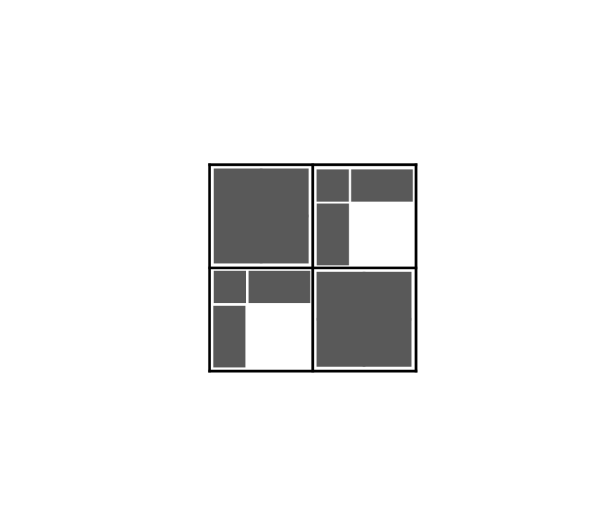
(c) merge children

(d) Start factorization

(e) $\ell=3$ skeletonization

(f) $\ell=2$ skeletonization

(g) $\ell=1$ skeletonization

Figure 3: Top row, from left to right: original matrix $A$, skeletonization step zeroing the light gray shade DOFs of the matrix and maintaining the skeleton DOFs in dark gray, merging the skeletons with common parent node. Rows 2 to 5 show the active DOFs on the 1D domain $\Omega$ after each step of the factorization, on three successive levels of skeletonization on the tree $\mathcal{T}_{\Omega}$.

4.2 2D case

In the multidimensional case, we have constructed an $\mathcal{H}$-matrix approximation $\dot{S}\approx S\equiv K^{*}K$. Denoting $\dot{S}$ by ${A}$ in this subsection, we can invert such representation in a similar way to that of the hierarchical interpolative factorization [21], but exploiting the $\mathcal{H}$-matrix representation.

Similarly to the one-dimensional case, the factorization proceeds from the leaves level $\ell=L$ of the tree $\mathcal{T}_{\Omega}$ to level $\ell=1$ and performs the following three steps at each level $\ell$:

• Skeletonization of cells at level $\ell$. There are $q_{\ell}=2^{\ell}\times 2^{\ell}$ square cells at level $\ell$. For each cell $I$ we let $\mathcal{I}$ be the set of indices for the active DOFs in the cell. Then, for each set of indices $\mathcal{I}$, we define the matrix

  $$\bar{U}_{\ell;\mathcal{I}}=\begin{bmatrix}{A}_{\mathcal{B}\mathcal{I}}\\ \widetilde{U}_{\ell;\mathcal{I}}^{*}\\ \vdots\\ \widetilde{U}_{1;\mathcal{I}}^{*}\end{bmatrix},$$ (4.19)

  with ${A}_{\ell;\mathcal{B}\mathcal{I}}$ the block of matrix ${A}_{\ell}$ indexed by DOFs in $\mathcal{I}$ and $\mathcal{B}$, where $\mathcal{B}$ includes the active DOFs of the neighboring cells $J\in NL(I)$ in level $\ell$ of the tree, i.e. the near field of $I$. Denote $I_{\ell}$ the node containing the DOFs $\mathcal{I}$ at level $\ell$ of $T_{\Omega}$ and $m$ the number of nodes in $IL(I_{\ell})$. The submatrices of the form $\widetilde{U}_{\ell;I}$ contain the low rank bases at level $\ell$ for the low-rank approximation of subblocks ${A}_{\mathcal{J}_{\ell,i}\mathcal{I}_{\ell}}={U}_{\ell;\mathcal{J}_{\ell,i}\mathcal{I}_{\ell}}{B}_{\ell;\mathcal{J}_{\ell,i}\mathcal{I}_{\ell}}{U}_{\ell;\mathcal{J}_{\ell,i}\mathcal{I}_{\ell}}^{*}$ for all nodes $J_{\ell,i}\in IL(I_{\ell})$,

  $$\widetilde{U}_{\ell;I}=\begin{bmatrix}B_{\ell;\mathcal{J}_{\ell,1}\mathcal{I}_{\ell}}{U}_{\ell;\mathcal{J}_{\ell,1}\mathcal{I}}^{*}\\ B_{\ell;\mathcal{J}_{\ell,2}\mathcal{I}_{\ell}}{U}_{\ell;\mathcal{J}_{\ell,2}\mathcal{I}}^{*}\\ \vdots\\ B_{\ell;\mathcal{J}_{\ell,m}\mathcal{I}_{\ell}}{U}_{\ell;\mathcal{J}_{\ell,m}\mathcal{I}}^{*}\end{bmatrix},$$ (4.20)

  with ${U}_{\ell;\mathcal{J}_{\ell,i}\mathcal{I}}$ containing only the columns indexed by $\mathcal{I}$ from ${U}_{\ell;\mathcal{J}_{\ell,i}\mathcal{I}_{\ell}}$.

  Similar to the 1D case, we perform interpolative decomposition on $\bar{U}_{\ell,\mathcal{I}}$ (4.3) to obtain the corresponding interpolation matrix $T_{\mathcal{I}}$. Now one can apply the zeroing matrix ${Z}_{\mathcal{I}}$ (4.11) followed by Gaussian elimination to eliminate the redundant DOFs $\widetilde{\mathcal{I}}$ as in (4.13),

  $${M}_{\widetilde{\mathcal{I}}}^{*}{Z}_{\mathcal{I}}^{*}{A}_{\ell}{Z}_{\mathcal{I}}{M}_{\widetilde{\mathcal{I}}}\approx\begin{bmatrix}I&&\\ &{\bar{A}}_{\hat{\mathcal{I}}\hat{\mathcal{I}}}&{A}_{\mathcal{R}\hat{\mathcal{I}}}^{*}\\ &{A}_{\mathcal{R}\hat{\mathcal{I}}}&{A}_{\mathcal{R}\mathcal{R}}\\ \end{bmatrix}.$$ (4.21)

  Notice we are computing $T_{\mathcal{I}}$ using $\bar{U}_{\ell;\mathcal{I}}$ instead of the subblock ${A}_{\mathcal{R}\mathcal{I}}$. This is equivalent but essential to reduce the numerical complexity of the algorithm, since $\bar{U}_{\ell;\mathcal{I}}$ has many less rows than ${A}_{\mathcal{R}\mathcal{I}}$. In particular one can write ${A}_{\mathcal{R}\mathcal{I}}$ as

  $${A}_{\mathcal{R}\mathcal{I}}=\begin{bmatrix}I&&&\\ &V_{\ell;\mathcal{I}}&&\\ &&\ddots&\\ &&&V_{1;\mathcal{I}}\end{bmatrix}\begin{bmatrix}{A}_{\mathcal{B}\mathcal{I}}\\ \widetilde{U}_{\ell;\mathcal{I}}^{*}\\ \vdots\\ \widetilde{U}_{1;\mathcal{I}}^{*}\end{bmatrix}\equiv Q_{\ell;\mathcal{I}}\bar{U}_{\ell;\mathcal{I}}$$ (4.22)

  with $Q_{\ell;\mathcal{I}}$ having orthogonal columns and $V_{\ell;\mathcal{I}}$ containing the low-rank bases of all $m$ nodes in $IL(I_{\ell})$,

  $$V_{\ell;\mathcal{I}}=\begin{bmatrix}U_{\ell;\mathcal{J}_{1}\mathcal{I}_{\ell}}&&&\\ &U_{\ell;\mathcal{J}_{2}\mathcal{I}_{\ell}}&&\\ &&\ddots&\\ &&&U_{\ell;\mathcal{J}_{m}\mathcal{I}_{\ell}}\end{bmatrix}$$ (4.23)

  with $U_{\ell;\mathcal{J}_{i}\mathcal{I}_{\ell}}$ the block $U_{\ell;\mathcal{J}_{\ell,i}\mathcal{I}_{\ell}}$ (from the low-rank approximation $A_{\mathcal{J}_{\ell,i}\mathcal{I}_{\ell}}=U_{\ell;\mathcal{J}_{\ell,i}\mathcal{I}_{\ell}}B_{\ell;\mathcal{J}_{\ell,i}\mathcal{I}_{\ell}}U_{\ell;\mathcal{J}_{\ell,i}\mathcal{I}_{\ell}}^{*}$ in the $\mathcal{H}$-matrix representation) restricted to the rows indexed by the active DOFs of the node $J_{\ell,i}\in IL(I)$. Performing ID on $\bar{U}_{\ell;\mathcal{I}}$ gives an error

  $$\begin{split}\|E_{\mathcal{I}}\|=&\|{A}_{\mathcal{R}\widetilde{\mathcal{I}}}-{A}_{\mathcal{R}\hat{\mathcal{I}}}T_{\mathcal{I}}\|=\|Q_{\ell,\mathcal{I}}\bar{U}_{\ell;\widetilde{\mathcal{I}}}-Q_{\ell,\mathcal{I}}\bar{U}_{\ell;\hat{\mathcal{I}}}T_{\mathcal{I}}\|=\\ &\|\bar{U}_{\ell;\widetilde{\mathcal{I}}}-\bar{U}_{\ell;\hat{\mathcal{I}}}T_{\mathcal{I}}\|=O(\epsilon\|\bar{U}_{\ell,\mathcal{I}}\|)=O(\epsilon\|{A}_{\mathcal{R}\mathcal{I}}\|),\end{split}$$ (4.24)

  of the same order of magnitude that if ID had been performed on ${A}_{\mathcal{R}\mathcal{I}}$ directly, since $Q_{\ell,\mathcal{I}}$ has orthogonal columns, and therefore $\|{A}_{\mathcal{R}\mathcal{I}}\|=\|\bar{U}_{\ell,\mathcal{I}}\|$.

  Let $\{\mathcal{I}_{\ell,i}\}_{i=1}^{q_{\ell}}$ be the collection of disjoint index sets corresponding to active DOFs of each of the $q_{\ell}$ cells at level $\ell$. Performing skeletonization over all cells at level $\ell$ results in

  $${\bar{A}}_{\ell}\approx R_{\ell}^{*}{A}_{\ell}R_{\ell},\qquad R_{\ell}=\prod_{i=1}^{q_{\ell}}{Z}_{\mathcal{I}_{\ell,i}}E_{\widetilde{\mathcal{I}}_{\ell,i}},$$ (4.25)

  where we have decoupled all the redundant DOFs in the square cells. Now, the remaining active DOFs in ${\bar{A}}_{\ell}$ are $\cup_{i=1}^{q_{\ell}}\hat{\mathcal{I}}_{i}$, and the DOFs $\cup_{i=1}^{q_{\ell}}\widetilde{\mathcal{I}}_{i}$ have been decoupled, i.e. their corresponding matrix block in ${\bar{A}}_{\ell}$ is the identity matrix.

  Analogously to the 1D case, for each cell at a level $\ell$, with active DOFs indexed by $\mathcal{I}$, one can scale the off-diagonal low-rank bases with the Cholesky factor of ${A}_{\ell;\mathcal{I}\mathcal{I}}$ before computing the interpolative decomposition for improved accuracy of the factorization for ill-conditioned matrices.

• Skeletonization around the edges at level $\ell$. After performing cell skeletonization, most skeletons concentrate around the edges. This happens because of the high-rank interaction between the DOFs of adjacent cells located near a common edge. However, if these nodes are considered all together, then their interaction with the rest of the matrix can be assumed to be low-rank and we can reduce the number of skeleton DOFs around each edge.

  In order to take advantage of this behavior, we start by assigning every active DOF to the nearest edge at level $\ell$. Each edge will have DOFs assigned to it from two adjacent cells. For each edge, let $\mathcal{I}$ be the active DOFs assigned to it from adjacent cells. Then, we define the matrix

  $$\bar{U}_{\ell;\mathcal{I}}=\begin{bmatrix}{\bar{A}}_{\mathcal{B}\mathcal{I}_{1}}&{\bar{A}}_{\mathcal{B}\mathcal{I}_{2}}\\ \widetilde{U}_{\ell;\mathcal{I}_{1}}^{*}&\\ \vdots&\\ \widetilde{U}_{1;\mathcal{I}_{1}}^{*}&\\ &\widetilde{U}_{\ell;\mathcal{I}_{2}}^{*}\\ &\vdots\\ &\widetilde{U}_{1;\mathcal{I}_{2}}^{*}\\ \end{bmatrix}$$ (4.26)

  with $\mathcal{I}_{1}$ and $\mathcal{I}_{2}$ the indices of $\mathcal{I}$ corresponding to each of the two cells adjacent to the edge and subblocks $\widetilde{U}_{\ell,\mathcal{I}_{i}}$ defined as in (4.20). Here, $\mathcal{B}$ contains the DOFs in the union of the near field and the interior DOFs of the cells adjacent to the edge we are sparsifying. Now we can compute the interpolative decomposition of $\bar{U}_{\ell;\mathcal{I}}$ to construct the zeroing matrix ${Z}_{\mathcal{I}}$ (4.11) and decouple the redundant DOFs $\widetilde{\mathcal{I}}$ as in (4.13) with Gaussian elimination resulting in

  $${M}_{\widetilde{\mathcal{I}}}^{*}{Z}_{\mathcal{I}}^{*}{\bar{A}}_{\ell}{Z}_{\mathcal{I}}{M}_{\widetilde{\mathcal{I}}}\approx\begin{bmatrix}I&&\\ &\bar{{\bar{A}}}_{\hat{\mathcal{I}}\hat{\mathcal{I}}}&{\bar{A}}_{\mathcal{R}\hat{\mathcal{I}}}^{*}\\ &{\bar{A}}_{\mathcal{R}\hat{\mathcal{I}}}&{\bar{A}}_{\mathcal{R}\mathcal{R}}\\ \end{bmatrix}.$$ (4.27)

  One can decompose ${\bar{A}}_{\mathcal{R}\mathcal{I}}$ as

  $${\bar{A}}_{\mathcal{R}\mathcal{I}}=\begin{bmatrix}I&&&&&\\ &V_{\ell;\mathcal{I}_{1}}&&&V_{\ell;\mathcal{I}_{2}}&&\\ &&\ddots&&&\ddots&\\ &&&V_{1;\mathcal{I}_{1}}&&&V_{1;\mathcal{I}_{2}}\\ \end{bmatrix}\bar{U}_{\ell,\mathcal{I}}\equiv Q_{\ell,\mathcal{I}}\bar{U}_{\ell,\mathcal{I}}$$ (4.28)

  where $V_{\ell;\mathcal{I}_{1}}$ and $V_{\ell;\mathcal{I}_{2}}$ are defined as in (4.23). Analogously to cell skeletonization, the error committed with ID performed on $\bar{U}_{\ell;\mathcal{I}}$ is

  $$\begin{split}\|E_{\mathcal{I}}\|=&\|{A}_{\mathcal{R}\widetilde{\mathcal{I}}}-{A}_{\mathcal{R}\hat{\mathcal{I}}}T_{\mathcal{I}}\|=\|Q_{\ell,\mathcal{I}}\bar{U}_{\ell;\widetilde{\mathcal{I}}}-Q_{\ell,\mathcal{I}}\bar{U}_{\ell;\hat{\mathcal{I}}}T_{\mathcal{I}}\|\leq\\ &\sqrt{2}\|\bar{U}_{\ell;\widetilde{\mathcal{I}}}-\bar{U}_{\ell;\hat{\mathcal{I}}}T_{\mathcal{I}}\|=O(\epsilon\|\bar{U}_{\ell,\mathcal{I}}\|),\end{split}$$ (4.29)

  where we have used the fact $\|Q_{\ell,\mathcal{I}}\|\leq 2$. Since $Q_{\ell,\mathcal{I}}$ is a tall skinny matrix composed of two tall-skinny matrices ($Q_{\ell,\mathcal{I}}=[Q_{1},Q_{2}]$) with orthogonal columns, concatenated horizontally, it is trivial to bound its norm by

  $$\begin{split}\|(\begin{matrix}Q_{1}&Q_{2}\end{matrix})\|=&\max_{\|(\begin{matrix}v_{1}&v_{2}\end{matrix})\|=1}\|(\begin{matrix}Q_{1}&Q_{2}\end{matrix})(\begin{matrix}v_{1}&v_{2}\end{matrix})^{T}\|\leq\max_{\|(\begin{matrix}v_{1}&v_{2}\end{matrix})\|=1}\|Q_{1}v_{1}^{T}+Q_{2}v_{2}^{T}\|\leq\\ &\max_{\|(\begin{matrix}v_{1}&v_{2}\end{matrix})\|=1}\|Q_{1}v_{1}^{T}\|+\|Q_{2}v_{2}^{T}\|=\max_{\|(\begin{matrix}v_{1}&v_{2}\end{matrix})\|=1}\|v_{1}\|+\|v_{2}\|=\sqrt{2}.\end{split}$$ (4.30)

  Let $s_{\ell}$ be the number of edges and $\{\mathcal{I}_{\ell,i}\}_{i=1}^{s_{\ell}}$ the collection of corresponding disjoint index sets at level $\ell$, corresponding to each edge $i$. Performing skeletonization on all the index sets gives

  $${A}_{\ell-1}\approx\bar{R}_{\ell}^{T}{\bar{A}}_{\ell}\bar{R}_{\ell},\qquad\bar{R}_{\ell}=\prod_{i=1}^{s_{\ell}}{Z}_{\mathcal{I}_{\ell,i}}{M}_{\widetilde{\mathcal{I}}_{\ell,i}},$$ (4.31)

  where the remaining active DOFs in ${A}_{\ell-1}$ are $\mathcal{S}_{\ell-1}=\cup_{i=1}^{s_{\ell}}\hat{\mathcal{I}}_{\ell,i}$. The index sets $\cup_{i=1}^{s_{\ell}}\widetilde{\mathcal{I}}_{\ell,i}$ have been decoupled, i.e. their corresponding matrix block in ${A}_{\ell-1}$ is the identity matrix.

• Merge child blocks. After the skeletonization step on all edges, we merge the active DOFs of sibling nodes and move to the next level in the tree, i.e. to the parent node at level $\ell-1$ obtained from merging 4 adjacent square cells into a bigger square cell.

Similarly to the 1D case, at the end of the factorization we can approximate the inverse of the $\mathcal{H}$-matrix as

$$\dot{G}=R_{L}\bar{R}_{L}R_{L-1}\bar{R}_{L-1}\cdots R_{1}\bar{R}_{1}{A}_{L}^{-1}\bar{R}_{1}^{*}R_{1}^{*}\cdots\bar{R}_{L-1}^{*}R_{L-1}^{*}\bar{R}_{L}^{*}R_{L}^{*}\approx{A}^{-1}=(\dot{S})^{-1}\approx(K^{*}K)^{-1},$$ (4.32)

with $R_{\ell}$ and $\bar{R}_{\ell}$ the cell and edge skeletonization matrices at level $\ell$ respectively. The matrix $A_{L}$ defined at the root level can be easily inverted since it has few remaining active DOFs. Figure 4 illustrates the active DOFs concentrating around the edges and the vertices after each cell and edge skeletonization steps respectively, for two levels of the tree.

(a) factorization start

(b) face skeletonization

(c) edge skeletonization

(d) face skeletonization

(e) edge skeletonization

Figure 4: Active DOFs on the 2D square domain $\Omega$ for each step of the factorization, on two successive levels of the tree $\mathcal{T}_{\Omega}$

5 Approximate inverse factorization for FIOs

We now proceed to describe the algorithm for inverting the discrete FIO. Given that the discrete FIO matrix ${K}$ is square and invertible, we can obtain its inverse by computing the pseudo-inverse

$${K}^{-1}=(K^{*}{K})^{-1}K^{*}.$$ (5.1)

First, we approximate $K^{*}$ and ${K}$ using the butterfly factorization $\dot{K}\approx{K}$. Since the Hermitian matrix $K^{*}{K}$ has low-rank blocks for well separated clusters, we can use HODLR and $\mathcal{H}$-matrix representations in 1D and 2D respectively.

The HODLR (or $\mathcal{H}$-matrix) approximation $\dot{S}$ of $S\equiv K^{*}{K}$ is then computed using the peeling algorithm. Fast matrix-vector multiplications with ${K}^{*}{K}$ needed in the peeling algorithm are obtained by multiplying with $\dot{K}$ and $\dot{K}^{*}$, which can be done in quasi-linear time.

Next, we invert the hierarchical matrix approximation $\dot{S}$ of $K^{*}{K}$ using the inversion algorithm described in section 4, obtaining an approximate inverse $\dot{G}\approx(K^{*}{K})^{-1}$. Finally, we can construct the approximate factorization of the inverse FIO by approximating the terms $(K^{*}{K})^{-1}$ and $K^{*}$ in (5.1) with $\dot{G}$ and $\dot{K}^{*}$ respectively, i.e. ${K}^{-1}\approx\dot{G}\dot{K}^{*}$. The algorithm is summarized in Algorithm 1.

One can use the above factorization to get an approximate inverse, but for higher accuracy, $\dot{G}\dot{K}^{*}$ can be used as a preconditioner. If we want to solve a non-symmetric system of equations of the form ${K}Ff=u$ (1.7), we can first solve the system

$${K}\hat{f}=u$$ (5.2)

and then apply inverse FFT to $f$. In order to solve (5.2) efficiently, we can first approximate the FIO matrix by its butterfly factorization $\dot{K}\approx{K}$ so that matrix-vector multiplication can be performed in quasi-linear time. Next, we precondition the system with $\dot{G}\dot{K}^{*}$ and solve the approximate system

$$\dot{G}\dot{K}^{*}\dot{K}\hat{f}=\dot{G}\dot{K}^{*}u$$ (5.3)

for which we can run conjugate gradient [19] on the hermitian matrix $\dot{K}^{*}\dot{K}$ preconditioned with $\dot{G}$, $\text{pcg}(\dot{K}^{*}\dot{K},\text{ }\dot{K}^{*}u,\text{ }\dot{G})$.

Given: FIO phase function $\Phi(x,\xi)$, butterfly factorization tolerance $\epsilon_{BFF}$, peeling tolerance $\epsilon_{peel}$, HIF inversion tolerance $\epsilon_{HIF}$

$//$ Factor the FIO matrix ${K}$ with butterfly factorization with tolerance $\epsilon_{BFF}$

$\dot{K}\leftarrow\text{BFF}(\Phi(x,\xi),\epsilon_{BFF})$

$//$ Construct Hierarchical matrix representation of $K^{*}{K}$ with matrix peeling using fast matrix-vector multiplications with $F$ and tolerance $\epsilon_{peel}$

$\dot{S}\leftarrow\text{peeling}(\dot{K},\epsilon_{peel})$

$//$ Invert $\dot{S}$ with the hierarchical interpolative factorization

$\dot{G}\leftarrow\text{HIF}(\dot{S},\epsilon_{HIF})$

$//$ Construct the inverse FIO

${K}^{-1}\approx\dot{G}\dot{K}^{*}$

Algorithm 1 Inverse factorization of multidimensional FIOs

5.1 Computational complexity

The butterfly factorization $\dot{K}$ can be computed in $O(N^{3/2})$ time complexity, and its direct and transpose application to a vector $v$, $\dot{K}v$ and $\dot{K}^{*}v$, can be computed in quasi-linear time $O(N\log N)$.

The HODLR and $\mathcal{H}$-matrix approximation $\dot{S}$ of $K^{*}{K}$ can be constructed in $O(N\log^{2}N)$, since $\dot{K}^{*}\dot{K}$ can be applied in $O(N\log N)$ time to any arbitrary vector $v$ and we need to apply it to $O(\log N)$ proving matrices with size $N\times(k+c)$.

Finally, $\dot{S}$ can be inverted in $O(N\log^{2}N)$ time since during the factorization we need to perform interpolative decomposition on matrices resulting from concatenation of $O(\log N)$ submatrices. Such factorization can be applied in quasi-linear time $O(N\log\log N)$ according to [21].

Therefore, the computational complexity for computing a factorization for the inverse FIO matrix ${K}^{-1}$ is $O(N^{3/2})$ and its application to a vector is $O(N\log N)$. Table 2 summarizes the asymptotic complexity of each step in the construction and application of the inverse factorization of discrete FIOs.

Operation	Complexity
Construct $\dot{K}$	$O(N^{3/2})$
Apply $\dot{K}$ and $\dot{K}^{*}$ to a vector	$O(N\log N)$
Construct $\mathcal{H}$-matrix $\dot{S}$	$O(N\log^{2}N)$
Construct $\dot{G}$	$O(N\log^{2}N)$
Apply $\dot{G}$ to a vector	$O(N\log\log N)$
Apply $\dot{G}\dot{K}^{*}\approx{K}^{-1}$ to a vector	$O(N\log N)$

Table 2: Complexity estimates for different steps in the FIO inverse factorization

6 Numerical results

In this section, we demonstrate the effectiveness of the method for 1D and 2D FIOs. Here, we have considered a typical setting with periodic functions $a(x,\xi)$ and $\phi(x,\xi)$ on $x$, with $\Phi(x,\xi)=x\cdot\xi+\phi(x,\xi)$. This allows one to embed the problem in a periodic cell, chosen here to be $[0,1)^{d}$.

The factorization obtained to approximate the inverse operator is also used as a preconditioner to solve a system of equations of the form $\dot{K}x=b$. The performance of the preconditioner is compared with $\dot{K}^{*}$, which can also be used as a preconditioner. Notice that without a preconditioner any iterative solver will take too many iterations to converge due to the fact that eigenvalues are not clustered. In particular, we compare the number of conjugate gradient (CG) iterations of the system

$$\dot{K}^{*}\dot{K}x=\dot{K}^{*}b,$$ (6.1)

preconditioned with and without $\dot{G}$. The following quantities are used in the rest of the section to evaluate the performance of the preconditioner:

• $N$: total number of DOFs in the problem;

• $e_{a}$: the relative error of the butterfly approximation $\dot{K}$ of ${K}$, defined as $\|{K}-\dot{K}\|/\|{K}\|$;

• $\epsilon$: the tolerance used in the hierarchical matrix construction and inversion;

• $e_{s}$: the relative error of the approximation $\dot{G}\dot{K}^{*}$ of $K^{-1}$, defined as $\|I-\dot{G}\dot{K}^{*}K\|\geq\|K^{-1}-\dot{G}\dot{K}^{*}\|/\|K^{-1}\|$;

• $t_{s}$: total running time of CG to solve (6.1);

• $n_{i}$: the number of CG iterations with relative residual equal to $10^{-8}$.

The errors $e_{a}$ and $e_{s}$ are approximated using randomized power iteration [14, 24] to $10^{-2}$ relative precision. The butterfly factorization is computed using the code from [27].

Example 1. 1D FIO with uniform amplitude.

We begin with an example of a one-dimensional discrete FIO of the form

$$u(x)=\int_{\mathbb{R}}a(x)e^{2\pi i\Phi(x,\xi)}\hat{f}(\xi)\text{d}\xi$$ (6.2)

with uniform amplitude $a(x,\xi)=1$ and phase function $\Phi(x,\xi)$ given by

$$\Phi(x,\xi)=x\cdot\xi+c(x)|\xi|,\quad c(x)=(2+\sin(2\pi x))/8.$$ (6.3)

Discretizing $x$ and $\xi$ on $[0,1)$ and $[-N/2,N/2)$ with $N$ points,

$$x_{i}=(i-1)/N\quad\text{and}\quad\xi_{j}=j-1-N/2,$$ (6.4)

leads to the discrete system $u=Kf$, with $u_{i}=u(x_{i})$, $f_{j}=\hat{f}(\xi_{j})$ and $K_{ij}=e^{2\pi i\Phi(x_{i},\xi_{j})}$.

We compute the approximate inverse factorization with tolerance $\epsilon=10^{-3}$ and $\epsilon=10^{-6}$, leading to errors $e_{s}$ of the order between $10^{-3}$ and $10^{-6}$ as reported in Table 3. The factorization $\dot{G}\dot{K}^{*}$ is also a much more efficient preconditioner than the adjoint FIO matrix $\dot{K}^{*}$. For example, when $\epsilon=10^{-6}$ is used, CG converges in just 2 iterations instead of 28, leading to a reduction in time by a factor of approximately 7.

	$\dot{K}\approx{K}$	$\dot{G}\dot{K}^{*}\approx{K}^{-1}$				$\dot{K}^{*}\approx K^{*}$
$N$	$e_{a}$	$\epsilon$	$e_{s}$	$n_{i}$	$t_{s}$	$n_{i}$	$t_{s}$
1024	$3.59e-7$	$1e-6$	$4.32e-6$	2	$1.79e-2$	28	$1.17e-1$
		$1e-3$	$2.06e-3$	3	$2.68e-2$
4096	$4.77e-7$	$1e-6$	$8.71e-6$	2	$1.15e-1$	28	$7.97e-1$
		$1e-3$	$2.08e-3$	3	$1.63e-1$
16384	$5.49e-7$	$1e-6$	$2.73e-5$	2	$7.42e-1$	27	$4.68e+0$
		$1e-3$	$4.26e-3$	3	$9.02e-1$
65536	$7.87e-7$	$1e-6$	$9.56e-5$	2	$3.92e+0$	28	$2.72e+1$
		$1e-3$	$4.07e-3$	3	$4.83e+0$
262144	$8.90e-7$	$1e-6$	$2.89e-4$	2	$2.07e+1$	27	$1.25e+2$
		$1e-3$	$5.57e-3$	3	$2.33e+1$

Table 3: Numerical results for 1D uniform amplitude FIO using the approximate inverse $\dot{G}\dot{K}^{*}$ and the adjoint FIO matrix $\dot{K}^{*}$ as preconditioners for CG with tolerance $1e-8$.

Example 2. 1D FIO with variable amplitude.

Here, we consider the 1D FIO from the previous example with variable periodic amplitude $a(x,\xi)$ in $x$ on the interval $[0,1]$, defined by a mixture of Gaussians of the form

$$\sum_{k=0}^{n_{k}}e^{-\frac{(x-x_{k})^{2}+(\xi-\xi_{k})^{2}}{\sigma^{2}}},$$ (6.5)

where $\sigma^{2}$ is set to $0.1$ or $0.05$.

We report the results in Tables 4 and 5. We observe that when using a variable amplitude function, the adjoint FIO matrix $\dot{K}^{*}$ is not an efficient preconditioner, since CG requires a very large number of iterations to converge, while the approximate inverse $\dot{G}\dot{K}^{*}$ converges in just very few iterations, similar to Example 1. Additionally, the solve time with CG is 20 to 400 times lower depending on the tolerance $\epsilon$ and the amplitude function $a(x,\xi)$ used. In particular, if $\sigma^{2}$ is set to $0.05$ as in Table 5, $\dot{K}^{*}$ becomes a very bad preconditioner, requiring the use of an approximate factorization of $K^{-1}$. We observe that constructing the approximate inverse factorization takes $O(N^{3/2})$ complexity, while its application can be done in quasi-linear time, as illustrated in Figure 5.

	$\dot{K}\approx{K}$	$\dot{G}\dot{K}^{*}\approx{K}^{-1}$				$\dot{K}^{*}\approx K^{*}$
$N$	$e_{a}$	$\epsilon$	$e_{s}$	$n_{i}$	$t_{s}$	$n_{i}$	$t_{s}$
1024	$3.66e-7$	$1e-5$	$6.13e-5$	2	$1.90e-2$	173	$6.81e-1$
		$1e-3$	$3.79e-2$	3	$2.71e-2$
4096	$5.03e-7$	$1e-5$	$1.38e-4$	2	$1.25e-1$	200	$5.80e+0$
		$1e-3$	$5.69e-3$	3	$1.73e-1$
16384	$6.69e-7$	$1e-5$	$3.48e-4$	2	$7.38e-1$	205	$3.62e+1$
		$1e-3$	$8.52e-3$	3	$9.42e-1$
65536	$8.49e-7$	$1e-5$	$9.97e-4$	3	$5.18e+0$	207	$2.08e+2$
		$1e-3$	$8.45e-3$	3	$5.02e+0$
262144	$8.58e-7$	$1e-5$	$3.92e-3$	3	$3.05e+1$	207	$1.10e+3$
		$1e-3$	$1.45e-2$	4	$3.61e+1$

Table 4: Numerical results for 1D variable amplitude (with $\sigma^{2}=0.1$) FIO using the approximate inverse $\dot{G}\dot{K}^{*}$ and the adjoint FIO matrix $\dot{K}^{*}$ as preconditioners for CG with tolerance $1e-8$.

	$\dot{K}\approx{K}$	$\dot{G}\dot{K}^{*}\approx{K}^{-1}$				$\dot{K}^{*}\approx K^{*}$
$N$	$e_{a}$	$\epsilon$	$e_{s}$	$n_{i}$	$t_{s}$	$n_{i}$	$t_{s}$
1024	$3.33e-7$	$1e-4$	$3.11e-3$	3	$3.06e-2$	1020	$4.02e+0$
		$1e-3$	$1.02e-2$	4	$3.84e-2$
4096	$4.10e-7$	$1e-4$	$5.57e-3$	3	$1.88e-1$	2221	$6.43e+1$
		$1e-3$	$1.24e-1$	4	$2.22e-1$
16384	$7.08e-7$	$1e-4$	$1.37e-2$	4	$1.20e+0$	2517	$4.29e+2$
		$1e-3$	$2.45e-2$	4	$1.33e+0$
65536	$7.51e-7$	$1e-4$	$1.87e-2$	4	$6.15e+0$	2630	$2.34e+3$
		$1e-3$	$4.46e-2$	5	$7.98e+0$
262144	$7.29e-7$	$1e-4$	$6.36e-2$	5	$3.38e+1$	2668	$1.13e+4$
		$1e-3$	$1.75e-1$	7	$4.39e+1$

Table 5: Numerical results for 1D variable amplitude (with $\sigma^{2}=0.05$) FIO using the approximate inverse $\dot{G}\dot{K}^{*}$ and the adjoint FIO matrix $\dot{K}^{*}$ as preconditioners for CG with tolerance $1e-8$.

Figure 5: Scaling results for 1D FIO from Example 2 with $\sigma^{2}=0.1$ and $\epsilon=0.001$. Timings are provided for each step of the algorithm to build the inverse factorization as well as the timings for matrix-vector multiplications with the resulting factorization. Reference $O(N)$ and $O(N^{3/2})$ lines are plotted, with dashed lines $--$ and $-\cdot-$, respectively.

Example 3. 2D generalized Radon transform.

Finally, we consider the 2D analog of the numerical Example 1,

$$u(x)=\sum_{\xi\in\Omega}e^{2\pi i\Phi(x,\xi)}\hat{f}(\xi),\quad x\in X$$ (6.6)

with phase function $\Phi(x,\xi)$ defined as

$$\begin{split}\Phi(x,\xi)=x\cdot\xi+\sqrt{c_{1}^{2}(x)\xi_{1}^{2}+c_{2}^{2}(x)\xi_{2}^{2}},\\ c_{1}(x)=(2+\sin(2\pi x_{1})\sin(2\pi x_{2}))/16,\\ c_{2}(x)=(2+\cos(2\pi x_{1})\cos(2\pi x_{2}))/16,\end{split}$$ (6.7)

and

$$X=\left\{x=\Big{(}\frac{n_{1}}{n},\frac{n_{2}}{n}\Big{)},0\leq n_{1},n_{2}<n,\text{ with }n_{1},n_{2}\in\mathbb{Z}\right\},$$ (6.8)

$$\Omega=\left\{\xi=(n_{1},n_{2}),-\frac{n}{2}\leq n_{1},n_{2}<\frac{n}{2},\text{ with }n_{1},n_{2}\in\mathbb{Z}\right\},$$ (6.9)

with $n$ being the number of points in each dimension and $N=n^{2}$. This leads again to the system $u=Kf$ with $K=(e^{2\pi i\Phi(x,\xi)})_{x\in X,\xi\in\Omega}$, for which we are interested in the inversion of matrix $K$ and the solution $f=K^{-1}u$. This FIO models an integration over ellipses centered at a point $x\in X$ with axis lengths defined by $c_{1}(x)$ and $c_{2}(x)$.

One can use the butterfly factorization to obtain a factorization $\dot{K}$ of $K$ with forward error $e_{a}$ between $10^{-4}$ and $10^{-5}$. As observed in Table 6, using tolerance $\epsilon=10^{-3}$ for the peeling algorithm and the $\mathcal{H}$-matrix inversion we can find an approximate inverse factorization that is $\epsilon$-accurate. This factorization of the inverse can be used as direct solver or as a preconditioner for CG, which converges in just 3 iterations, as opposed to the 20 iterations needed when only $\dot{K}^{*}$ is used. Notice also that the total timing of CG is 4 times lower. The timings for the different parts of the algorithm are illustrated in Figure 6. We observe $O(N^{3/2})$ time complexity for building the factorization and almost $O(N)$ time for performing matrix–vector multiplication. The algorithm proposed for $\mathcal{H}$-matrix inversion experimentally shows quasi-linear complexity.

	$\dot{K}\approx{K}$	$\dot{G}\dot{K}^{*}\approx{K}^{-1}$				$\dot{K}^{*}\approx K^{*}$
$N$	$e_{a}$	$\epsilon$	$e_{s}$	$n_{i}$	$t_{s}$	$n_{i}$	$t_{s}$
$64^{2}$	$9.62e-5$	$1e-3$	$2.13e-3$	3	$7.09e-1$	20	$1.36e+0$
$128^{2}$	$9.72e-5$	$1e-3$	$2.64e-3$	3	$4.25e+0$	21	$1.56e+1$
$256^{2}$	$2.05e-4$	$1e-3$	$4.75e-3$	3	$2.27e+1$	22	$7.6e+1$
$512^{2}$	$2.27e-4$	$1e-3$	$9.46e-3$	4	$1.87e+2$	22	$6.5e+2$

Table 6: Numerical results for 2D FIO using the approximate inverse $\dot{G}\dot{K}^{*}$ and the adjoint FIO matrix $\dot{K}^{*}$ as preconditioners with tolerance $1e-8$.

Figure 6: Scaling results for 2D FIO with $\epsilon=0.001$. Timings are provided for constructing BFF and $\mathcal{H}$-matrix as well as for inverting the $\mathcal{H}$-matrix and performing matrix-vector multiplications with the factorizations of $\dot{G}$ and $\dot{G}\dot{K}^{*}$. Reference $O(N)$ and $O(N^{3/2})$ lines are plotted, with dashed lines $--$ and $-\cdot-$ respectively.

7 Conclusions

In this paper, we have introduced an algorithm to obtain a factorization of inverse discrete FIO matrices $K\in\mathbb{C}^{N\times N}$ in 1D and 2D that can be computed in $O(N^{3/2})$ time and space complexity. The algorithm combines the butterfly factorization with hierarchical matrices, to exploit the complimentary low-rank condition of discrete FIO matrices $K$ and the numerical low-rank subblocks that appear in the corresponding hermitian matrix $K^{*}K$. With such factorization, the inverse matrix $K^{-1}$ is represented as a product of $O(\log N)$ sparse matrices, and therefore it can be applied in quasi-linear time, $O(N\log N)$. This factorization can be used either as a direct solver or as a preconditioner for iterative methods depending on the accuracy required. When used as a preconditioner the factorization can reduce the number of iterations of iterative methods such as CG or GMRES, which otherwise can take $O(N)$ iterations to converge. We have also proposed a new algorithm to invert HODLR and $\mathcal{H}$-matrix representations based on recursive skeletonization and HIF, that construct approximate inverse factorizations in quasi-linear time.

Notice that the three main steps of the algorithm (butterfly factorization, $\mathcal{H}$-matrix construction and $\mathcal{H}$-matrix inversion) can be easily parallelized. The butterfly factorization and $\mathcal{H}$-matrix inversion algorithms are organized following a tree structure, where at a each level every node can be processed independently of the rest, as done in [26]. Similarly, the $\mathcal{H}$-matrix construction for the 2D case can be easily parallelized at each level of the tree with 64 processors, one for each subset $\mathcal{P}_{p,q}$ in (3.16).

The algorithm proposed here can also be used on higher dimensions ($d>2$) by partitioning the domain in $d-$dimensional hypercubes, as far as admissible blocks on $K^{*}K$ can be considered low-rank.

References

• [1] A. Aminfar, S. Ambikasaran, and E. Darve, A fast block low-rank dense solver with applications to finite-element matrices, J. Comput. Phys., 304:170–188, 2016.
• [2] S. Ambikasaran, and E. Darve, An $O(N\log N)$ fast direct solver for partial hierarchically semi-separable matrices, J. Sci. Comput., 57:477–501, 2013.
• [3] M. Bebendorf, M. Bollhöfer, and M. Bratsch, Hierarchical matrix approximation with blockwise constraints, BIT Numer. Math., 53(2):311–339, 2013.
• [4] G. Beylkin, R. Coifman, and V. Rokhlin. Fast wavelet transforms and numerical algorithms, I. Commun. on Pure Appl. Math., 44(2):141–183, 1991.
• [5] A. Brandt, Multi-level adaptive solutions to boundary-value problems, Math. Comp., 31(138):333–390, 1977.
• [6] E. Candés, L. Demanet, and L. Ying. A fast butterfly algorithm for the computation of Fourier integral operators: Multiscale Model and Simulation, 7:1727–1750, 2009.
• [7] E. Candés, L. Demanet, and L. Ying. Fast Computation of Fourier Integral Operators, SIAM J. Sci. Comput., 29(6): 2464–2493, 2007.
• [8] Z. Chen, J.  Zhang, K. L. Ho, and H. Yang Multidimensional phase recovery and interpolative decomposition butterfly factorization, J. Comput. Phys., 412:109427, 2020.
• [9] M. Cheney, and B. Borden. Fundamentals of radar imaging, SIAM, 2009.
• [10] H. Cheng, Z. Gimbutas, P. G. Martinsson, and V. Rokhlin, On the compression of low rank matrices, SIAM J. Sci. Comput., 26(4):1389–1404, 2005.
• [11] E. Corona, P.-G. Martinsson, and D. Zorin, An $O(N)$ direct solver for integral equations on the plane, Appl. Comput. Harmon. Anal., 38(2):284–317, 2015.
• [12] L. Demanet and L. Ying, Fast wave computation via Fourier integral operators, Math. Comp., 81:1455–1486, 2012.
• [13] P. Coulier, H. Pouransari, and E. Darve, The inverse fast multipole method: Using a fast approximate direct solver as a preconditioner for dense linear systems, SIAM J. Sci. Comput., 39(3):A761–A796, 2017.
• [14] J. D. Dixon, Estimating extremal eigenvalues and condition numbers of matrices, SIAM J. Numer. Anal., 20(4):812–814, 1983.
• [15] G. H. Golub and C. F. van Loan,Matrix Computations, Johns Hopkins, Baltimore, 3rd edition, 1996.
• [16] W. Hackbusch, A sparse matrix arithmetic based on $\mathcal{H}$-matrices. Part I: Introduction to $\mathcal{H}$-matrices, Computing, 62:89–108, 1999.
• [17] W. Hackbusch and S. Börn, Data-sparse approximation by adaptive $\mathcal{H}^{2}$-matrices, Computing, 69:1–35, 2002.
• [18] N. Halko, P. G. Martinsson, and J. A. Tropp, Finding structure with randomness: Probabilistic algorithms for constructing approximate matrix decompositions, SIAM Rev., 53:217–288, 2011.
• [19] M. R. Hestenes, and E. Stiefel, Methods of conjugate gradients for solving linear systems, J. Res. Natl. Bur. Standards, 49:409–436, 1952.
• [20] K. L. Ho, and L. Greengard, A fast direct solver for structured linear systems by recursive skeletonization, SIAM J. Sci. Comput., 34(5):A2507–A2532, 2012.
• [21] K. L. Ho, and L. Ying, Hierarchical interpolative factorization for elliptic operators: Integral equations, Comm. Pure Appl. Math., 69(7):1314–1353, 2016.
• [22] J. Hu, S. Fomel, L. Demanet, and L. Ying, A fast butterfly algorithm for generalized Radon transforms, Geophysics, 78:U41–U51, 2013.
• [23] P. Kuchment, and L. Kunyansky, Mathematics of thermoacoustic tomography, European J. Appl. Math., 19(2):191–224, 2008.
• [24] J. Kuczyński and H. Woźniakowski, Estimating the largest eigenvalue by the power and Lanczos algorithms with a random start, SIAM J. Matrix Anal. Appl., 13(4):1094–1122, 1992.
• [25] L. Kunyansky, Inversion of the 3-D exponential parallel-beam transform and Radon transform with angle-dependent attenuation, Inverse Problems, 20:1455–1478, 2004.
• [26] Y. Li, and L. Ying, Distributed-memory hierarchical interpolative factorization, Res. Math. Sci., 4(12), 2017.
• [27] Y. Li, Butterfly factorization, https://github.com/YingzhouLi/BF.m, 2016.
• [28] Y. Li, H. Yang, E. Martin, K. Ho, and L. Ying, Butterfly factorization, Multiscale Model. Simul. 13(2):714–732, 2015.
• [29] Y. Li, H. Yang, L. Ying, A multiscale butterfly algorithm factorization, Applied and Computational Harmonic Analysis, 44(3):737–758, 2018.
• [30] Y. Li, H. Yang Interpolative butterfly factorization, SIAM J. Sci. Comput., 39(2):A503–A531, 2017.
• [31] L. Lin, J. Lu, and L. Ying, Fast construction of hierarchical matrix representation from matrix-vector multiplication, J. Comput. Phys., 230:4071–4087, 2011.
• [32] Y. Liu, X. Xing, H. Guo, E. Michielssen, P. Ghysels, and X. S. Li, Butterfly factorization via randomized matrix-vector multiplications, arXiv:2002.03400 [math.NA], 2020.
• [33] P. G. Martinsson and V. Rokhlin, A fast direct solver for boundary integral equations in two dimensions, J. Comput. Phys., 205(1):1–23, 2005.
• [34] P. G. Martinsson, A fast randomized algorithm for computing a hierarchically semiseparable representation of a matrix, SIAM J. Matrix Anal. Appl., 32:1251–1274, 2011.
• [35] E. Michielssen, and A. Boag, A multilevel matrix decomposition algorithm for analyzing scattering from large structures, IEEE Trans. Antennas and Propagation, 44(8):1086–1093, 1996.
• [36] V. Minden, K. L. Ho, A. Damle, and L. Ying, A recursive skeletonization factorization based on strong admissibility, Multiscale Model. Simul., 15(2):768–796, 2017.
• [37] Q. Pang, K. L. Ho, H. Yang, Interpolative decomposition butterfly factorization, SIAM J. Sci. Comput., 42(2):A1097-A1115, 2020.
• [38] J. Radon, Über die bestimmung von funktionen durch ihre integralwerte langs gewisser mannigfaltigkeiten: Berichte über die Verhandlungen der Sachsische Akademie der Wissenschaften, Reports on the proceedings of the Saxony Academy of Science, 69:262–277, 1917.
• [39] Y. Saad, Iterative Methods for Sparse Linear Systems, SIAM, Philadelphia, 2nd edition, 2003.
• [40] Y. Saad, M. H. Schultz GMRES: a generalized minimal residual algorithm for solving nonsymmetric linear systems, SIAM J. Sci. Stat. Comput, 7:856–869, 1986.
• [41] F. Santosa, M. Vogelius, Backprojection algorithm for electrical impedance imaging, SIAM J. Appl. Math. 50(1):216–243, 1990.
• [42] P. Stefanov, and G. Uhlmann, Thermoacoustic tomography arising in brain imaging, Inverse Problems 27:045004, 2011.
• [43] E. M. Stein, Harmonic Analysis: Real-Variable Methods, Orthogonality, and Oscillatory Integrals, Princeton Math. Ser. 43, Princeton University Press, Princeton, 1993.
• [44] W. W. Symes, Topical review: The seismic reflection inverse problem, Inverse Problems, 25(12):123008, 2009.
• [45] H. A. Van der Vorst, Bi-CGSTAB: A Fast and Smoothly Converging Variant of Bi-CG for the Solution of Nonsymmetric Linear Systems, SIAM J. Sci. Stat. Comput., 13(2):631–644, 1992.
• [46] J. Xia and Z.-X. Xing, Effective and robust preconditioning of general spd matrices via structured incomplete factorization, SIAM J. Matrix Analysis Applications, 38:1298–1322, 2017.
• [47] J. Xia, S. Chandrasekaran, M. Gu, and X. S. Li, Fast algorithms for hierarchically semiseparable matrices, Numer. Linear Algebra Appl., 17:953–976, 2010.
• [48] X. Xing and E. Chow, Preserving positive definiteness in hierarchically semiseparable matrix approximations, SIAM J. Matrix Anal. Appl., 39(2):829–855, 2018.
• [49] B. Yazici, L. Wang, and K. Duman, Synthetic aperture inversion with sparsity constraints, in Proceedings of the International Conference on Electromagnetics in Advanced Applications (ICEAA), 1404–1407, 2011.