Abstract

Applying an operator product expansion approach we update the Standard Model prediction of the $B_{c}$ lifetime from over 20 years ago. The non-perturbative velocity expansion is carried out up to third order in the relative velocity of the heavy quarks. The scheme dependence is studied using three different mass schemes for the $\bar{b}$ and $c$ quarks, resulting in three different values consistent with each other and with experiment. Special focus has been laid on renormalon cancellation in the computation. Uncertainties resulting from scale dependence, neglecting the strange quark mass, non-perturbative matrix elements and parametric uncertainties are discussed in detail. The resulting uncertainties are still rather large compared to the experimental ones, and therefore do not allow for clear-cut conclusions concerning New Physics effects in the $B_{c}$ decay.

1 Introduction

The $B_{c}$ meson is the lightest state with both “naked” beauty and charm. As such it is stable against both strong and electromagnetic decay. Its weak decay can proceed through three distinct mechanisms: either $\bar{b}$-quark decay, $c$-quark decay or $\bar{b}$-$c$ annihilation. Experimentally, the $B_{c}$ lifetime has been measured by LHCb [1, 2] and CMS [3] with a world average of [4]:

$$\tau_{B_{c}}^{\rm exp}=0.510(9)~{}\text{ps}\,,$$ (1)

which corresponds to a decay width

$$\Gamma_{B_{c}}^{\rm exp}=1.961(35)~{}\text{ps}^{-1}\,.$$ (2)

Since both valence quarks in the $B_{c}$ meson are heavy, the state is similar in structure to it’s quarkonium cousins, the $\eta_{c}$ and $\eta_{b}$ pseudoscalar mesons, the lightest members of the $J/\psi$ and $\Upsilon$ towers of states. This circumstance allows for an effective treatment in terms of Non-Relativistic QCD (NRQCD), where (much as in the case of heavy quarkonium) the anti-quark corresponding to the valence quark, or the quark corresponding to the valence anti-quark, is integrated out at the respective scale. This method has been used to estimate the lifetime of the $B_{c}$ meson in the Standard Model (SM) [5, 6, 7].

The most precise value has been obtained in [6] to be $\tau_{B_{c}}=0.52\,\text{ps}$, with an uncertainty from varying the input charm quark mass that results in $0.4\,\text{ps}<\tau_{B_{c}}<0.7\,\text{ps}$, corresponding to

$$\Gamma_{B_{c}}=1.92^{+0.58}_{-0.49}~{}\text{ps}^{-1}\,,$$ (3)

exclusive of other sources of uncertainty that include, among others, $\pm 22\%$ from scale uncertainty in the perturbative calculation.

Similar results were found in other OPE calculations [5, 7] as well as using QCD sum rules [8] or potential models [9]. A comparison of the different predictions can be found in [10].

The experimental measurement in Eq. (1) has a much smaller uncertainty than the theory prediction in Eq. (3). This motivates a reinvestigation of the SM prediction from over 20 years ago with the goal of improving the theoretical precision, and the eventual hope of a precision comparable to the experimental one.

Renewed interest in the $B_{c}$ lifetime has arisen because it is susceptible to New Physics (NP) effects. Consequently a more precise SM prediction allows to place stronger constrains on NP models. In particular, experimentally measured deviations from SM expectations in the semileptonic decays $B\to D\tau\nu$, $B\to D^{*}\tau\nu$ and $B_{c}\to\psi\tau\nu$ suggest NP contributions to the quark level process $b\to c\tau\nu$ [11, 12, 13, 14, 15, 16, 17]. These so-called $R(D)$, $R(D^{*})$ and $R(B_{c})$ anomalies can be accounted for by several extensions of the SM. If the NP is realized as an effective pseudoscalar interaction, that is, a four-fermion interaction involving a pseudoscalar hadronic bilinear times a leptonic $S-P$ bilinear, then the $B_{c}$ lifetime is especially effective in placing constraints on its strength [18, 19]. This type of interaction is often found in models of NP proposed in the interpretation of the $R(D^{(*)})$ anomalies, such as the two-Higgs-doublet model (2HDM) and leptoquarks. The $B_{c}$ lifetime constraint rules out any of the 2HDM interpretations of $R(D^{*})$, including the type III versions of the model that contain general Yukawa couplings to the different fermions [20], which can explain simultaneously $R(D)$ and $R(D^{*})$, [21, 22, 23, 24, 25, 26], going beyond the more restricted set of models [27, 28, 29, 30] on which BaBar [11, 12] and Belle [14] place constraints. Leptoquark models have also been proposed to explain these anomalies and they are susceptible to these bounds when they generate sizable pseudo-scalar operators [31, 18].

In this work we follow the OPE methodology of Ref. [6] (henceforth “BB”). There are several ways in which we can improve the result of that work. First and foremost, we use and compare three mass schemes to eliminate pole (or “on-shell”) masses in favor of well defined masses and therefore eliminate renormalon ambiguities that arise in the on-shell scheme. The largest source of uncertainty in the calculation of the width is from the pole masses, since the width scales as the fifth power of these. BB use ad hoc values for $b$ and $c$ pole masses. We perform the calculation in the $\overline{\text{MS}}$ mass scheme, the “Upsilon” scheme [32, 33], and a “meson” scheme that incorporates some aspects of the Upsilon scheme. We will expand on these below but for now we point out that the Upsilon scheme organizes the perturbative expansion in a manner that not only eliminates renormalon ambiguities from the expression for the decay width but in addition is empirically seen to have better convergence than other schemes. Moreover, the masses of the $\Upsilon$ and $J/\psi$ particles, used as inputs, are determined accurately. Second, for the one-loop calculation of the subprocess $b\to c\bar{c}s$ BB uses the result of Bagan et al [34, 35]. Later, Krinner, Lenz and Rauh (henceforth KLR) inferred the presence of typos in the analytic expressions of Bagan et al [36], because those expressions do not produce the numerical results and graphs they present. KLR compute the 1-loop corrections anew and agree with the numerical results of Bagan et al, inferring thus the presence of typos. We have used, and verified partially, the results of KLR. Third, BB neglect, and we include, the contribution of penguin operators, that are formally of the same order as other contributions retained in the calculation albeit numerically small. Fourth, we use better determined input parameters, such as the strong coupling constant $\alpha_{s}(M_{Z})$, the CKM matrix elements, and the non-perturbative $B_{c}$ decay constant, $f_{B_{c}}$, for which there is now a lattice calculation [37], among others. Fifth, we use spin symmetry to relate some of the non-perturbative matrix elements appearing in the calculation.

In addition to updating and improving on the BB result, we have tried to clarify several issues in their presentation. Among these we clarify below the need to go up to fourth order in velocity in the NREFT, the role of spin symmetry in the calculation of matrix elements, the relative (un)importance of various corrections, the distinction between quarks and anti-quarks in the NREFT as well as the interpretation and precise value of the momenta $p_{b}\pm p_{c}$ that enter the operators in the OPE for weak annihilation (WA) and Pauli interference (PI) diagrams.

The rest of the paper is organized as follows: In Sec. 2 the different mass schemes used for the calculation are discussed. In Sec. 3 we outline the Effective Field Theory approach used at the electroweak (EW) scale involving the effective Hamiltonian. The matching onto NRQCD is performed in Sec. 4. The Operator Product Expansion (OPE) is discussed in Sec. 5. Section 6 describes the computation of relevant matrix elements and in Sec. 7 the numerical computation and analysis of the uncertainties for the SM prediction is performed before we summarize our results and offer some observations in the conclusions, in Sec. 8.

2 Mass schemes

The largest source of uncertainty in the calculation of the inclusive rate of the $B_{c}$ decay is in the value of the pole mass. As we will review below, the calculation of the rate, $\Gamma_{B_{c}}$, is based on an OPE of the two point function of the effective Hamiltonian, cf Eqs. (33) and (34). The leading term in the calculation corresponds to $\Gamma_{b}+\Gamma_{c}$, the sum of decay rates of $b$ and $c$ quarks computed perturbatively as if the quarks were not bound to the $B_{c}$ meson. The rate $\Gamma_{q}$ is given in terms of the pole mass, $m_{q}$, as an expansion in powers of $\alpha_{s}$

$$\Gamma_{q}=\kappa m_{q}^{5}(f_{0}(x)+\epsilon\alpha_{s}f_{1}(x)+\epsilon^{2}\alpha_{s}^{2}f_{2}(x)+\cdots)\,,$$ (4)

where $\kappa$ is a constant independent of $m_{q}$, $x$ and $\alpha_{s}$ chosen so that the tree-level rate has $f_{0}(0)=1$. For reasons that will be explained momentarily, we have introduced the power counting parameter $\epsilon=1$ that is set to unity at the end of the calculation. The coefficients of the expansion, $f_{i}(x)$ are functions of the ratios of final state pole masses, $m_{q^{\prime}}$, to the mass of the decaying quark, $x=m_{q^{\prime}}/m_{q}$. Pole masses are convenient for the perturbative calculations, but are beset by both computational and conceptual difficulties: their perturbative expansion is poorly convergent and suffers from a renormalon ambiguity. Moreover, the roots of the implicit equation that relates them to short distance (Lagrangian) masses are complex for the light quarks.

When expressed in terms of the pole mass, the perturbative rate also suffers from a renormalon ambiguity. Remarkably, eliminating the pole mass in favour of well defined (e.g., short distance) masses, gives a perturbative expansion of the rate that is free of renormalon ambiguities [38, 39, 40, 41]. For each choice of well defined mass the manner in which renormalon ambiguities cancel in the rate suggests how to organize the perturbative expansion. We refer to any one choice of mass and of reorganization of the perturbative series as a “mass-scheme”. When the well defined quark masses are chosen as the modified minimally subtracted masses, $\overline{m}_{q}$, the expansion of the pole mass takes the form

$$m_{q}=\overline{m}_{q}(1+\epsilon\alpha_{s}d_{q}^{(1)}+\epsilon^{2}\alpha_{s}^{2}d_{q}^{(2)}+\cdots)\,,$$ (5)

so that the renormalon free expansion for the rate for the flavour transition $q\to q^{\prime}$ takes the form

$$\Gamma_{q\to q^{\prime}}=\kappa\overline{m}_{q}^{5}\left[f_{0}(\bar{x})+\epsilon\alpha_{s}\left(5d_{q}^{(1)}f_{0}(\bar{x})+(d_{q^{\prime}}^{(1)}-d_{q}^{(1)})\bar{x}\frac{df_{0}(\bar{x})}{d\bar{x}}+f_{1}(\bar{x})\right)+\mathcal{O}(\epsilon^{2})\right]\,,$$ (6)

where $\bar{x}=\overline{m}_{q^{\prime}}/\overline{m}_{q}$. As we see, in this “$\overline{\text{MS}}$ scheme” the expansion in $\epsilon$ is equivalent to the perturbative expansion in powers of $\alpha_{s}$.

By contrast, in the “Upsilon scheme” the power counting in $\epsilon$ does not correspond to powers of $\alpha_{s}$. Up to small non-perturbative corrections the $q$ pole mass is given in terms of that of the mass $M_{\bar{q}q}$ of some quarkonium $\bar{q}q$ state by

$$m_{q}=\tfrac{1}{2}M_{\bar{q}q}(1+\epsilon\alpha_{s}^{2}D_{q}^{(1)}+\epsilon^{2}\alpha_{s}^{3}D_{q}^{(2)}+\cdots)\,.$$ (7)

For example, if in $\Gamma_{b\to cud}$ we neglect the light quark masses and use this scheme for both $b$ and $c$ quarks, then

$$\Gamma_{b\to cud}=\kappa\left(\frac{M_{\bar{b}b}}{2}\right)^{5}\left\{f_{0}(X)+\epsilon\left[\alpha_{s}^{2}\left(5D_{b}^{(1)}f_{0}(X)+(D_{c}^{(1)}-D_{b}^{(1)})X\frac{df_{0}(X)}{dX}\right)+\alpha_{s}f_{1}(X)\right]\right.\\ \left.\phantom{\frac{df_{0}(X)}{dX}}+\mathcal{O}(\epsilon^{2})\right\}\,,$$ (8)

where now $X=M_{\bar{c}c}/M_{\bar{b}b}$.

While any good choice of well defined masses yields a well behaved perturbative expansion in the sense that it is free of renormalon ambiguities, different mass-schemes may differ in how rapidly the expansion converges (in the asymptotic expansion sense). Were we able to compute to high order, all mass-schemes would give the same numerical value for the rate (up to a small higher order term). But computations of rates are available only to low orders in perturbation theory, often only including 1-loop corrections to the leading, tree level term. In practical term it is best to choose a scheme that converges most rapidly. In the sub-sections below we present and compare the three schemes in which we perform calculations.

As stated above, the leading term in the OPE for the decay width of $B_{c}$ mesons is the perturbative $\Gamma_{b}+\Gamma_{c}$. The corrections to those are expressed as products of non-perturbative matrix elements and Wilson coefficients. The latter are perturbatively computed as functions of pole masses. In the calculations below we use the same scheme choice for these sub-leading terms as for the leading ones.

2.1 The $\overline{\text{MS}}$ mass-scheme

This scheme uses the running renormalized Lagrangian masses $\overline{m}_{b}(\mu)$ and $\overline{m}_{c}(\mu)$ evaluated at a sufficiently high renormalization scale $\mu$. In this scheme the expansion parameter $\epsilon$ simply counts powers of $\alpha_{s}$, making its use particularly simple. The expansion of $m_{b,c}$ in terms of the $\overline{\text{MS}}$ masses is known to third order in $\alpha_{s}$ [42, 43], but we only need it to first order:

$$m_{q}=\overline{m}_{q}(\mu)\left[1+\epsilon\frac{\alpha_{s}(\mu)}{\pi}\left(\frac{4}{3}-\ln\left(\frac{\overline{m}_{q}(\mu)^{2}}{\mu^{2}}\right)\right)\right]+\mathcal{O}(\alpha_{s}^{2})\,,$$ (9)

where we have retained explicitly the power of $\epsilon$ used in organizing the perturbative expansion, corresponding to Eq. (5). It is convenient to cast the $c$-quark decay rate in terms of the running mass evaluated at itself, $\overline{m}_{c}(\overline{m}_{c})$, and the $b$-quark decay rate in terms of both quark masses evaluated at the shorter distance scale, $\overline{m}_{b}(\overline{m}_{b})$ and $\overline{m}_{c}(\overline{m}_{b})$. The value of the masses, $\overline{m}_{b}(\overline{m}_{b})$ and $\overline{m}_{c}(\overline{m}_{c})$, is reported by the PDG with 1%-2% accuracy. Because the rates scale as the fifth power of the mass, this results in an uncertainty of 5%-10%. In addition, as discussed below, the convergence of the perturbative series is slow in the case of semileptonic $b$ and $c$ decays, and there is no reason to suspect it is any better for non-leptonic decays.

2.2 The Upsilon scheme

The Upsilon expansion was introduced by Hoang, Ligeti and Manohar in Refs. [32, 33] (henceforth “HLM”) to address the largest source of uncertainty in the calculation of the inclusive rate of semileptonic $B$ and $D$ meson decays. The calculation of the rate for semileptonic $B$ decays is based on an operator product expansion of the two-point function of hadronic charged currents

$$i\int d^{4}x\,e^{iq\cdot x}\langle B|T(j^{\mu}(x)j^{\nu\dagger}(0))|B\rangle$$

in terms of operators in the Heavy Quark Effective Theory (HQET) [44]. The expansion is naturally given in inverse powers of the pole mass of the decaying heavy quark, and the resulting rate is proportional to the fifth power of the pole mass. In the Upsilon scheme the masses are chosen to be the well measured 1S masses, $M_{\bar{b}b}=m_{\Upsilon}$ and $M_{\bar{c}c}=m_{J/\psi}$, resulting in a negligible uncertainty in the decay rate from the value of these masses. The expansion of the pole masses in terms of $m_{\Upsilon}$ and $m_{J/\psi}$ has been determined to fourth order in $\alpha_{s}$, with corrections that start at order $\alpha_{s}^{2}$ [45, 46]:

$$\frac{\tfrac{1}{2}m_{\Upsilon}}{m_{b}}=1-\frac{(\alpha_{s}C_{F})^{2}}{8}\left\{1\epsilon+\frac{\alpha_{s}}{\pi}\left[\left(\ln\left(\frac{\mu}{\alpha_{s}C_{F}m_{b}}\right)+\frac{11}{6}\right)\beta_{0}-4\right]\epsilon^{2}+\cdots\right\}\,,$$ (10)

where $\beta_{0}=11-\frac{2}{3}n_{f}$ is the coefficient of the first term in the QCD $\beta$-function, $C_{F}=(N_{c}^{2}-1)/2N_{c}=4/3$, and we have omitted the known term of order $\alpha_{s}^{4}$. For quarkonium systems the quark potential suffers from a renormalon ambiguity, as does the pole mass, but the resulting quarkonium state energy is free from ambiguities and hence the onium mass is a good candidate for an unambiguous, well defined mass [47, 48].

The organization of the expansion is unusual. The parameter $\epsilon=1$ is inserted to indicate the order in the expansion. For the expansion of the rate in Eq. (4) the power of $\epsilon$ matches that of $\alpha_{s}$. But, as seen above, the parameter $\epsilon$ in Eq. (7) carries one additional power of $\alpha_{s}$, i.e., $\epsilon^{n}\alpha_{s}^{n+1}$. As seen in Eq. (8) the leading correction to the rate includes order $\alpha_{s}$ terms from the perturbative corrections to the rate, and order $\alpha_{s}^{2}$ from the perturbative expansion of the masses. This is dictated by the requirement that the renormalons cancel in the expression for the rate.

In the implementation of this scheme for non-leptonic decays HLM expand the Wilson coefficients of the electroweak effective Hamiltonian in powers of $\alpha_{s}\ln(m_{W}/m_{b})$ and truncate in the power of $\alpha_{s}$ to which they perform the calculation of the rate. We do not adopt this prescription and instead retain the full resummed values of the Wilson coefficients. The reason is that this series does not contribute to the cancellation of renormalons, as can be seen from the fact that $M_{W}$ is an arbitrary parameter. This is the case for the other mass schemes as well.

2.3 The “meson” scheme

The HQET gives the heavy baryon masses as an expansion in inverse powers of the pole masses. To second order in the heavy quark expansion one has

$$m_{b}-m_{c}=\overline{m}_{B}-\overline{m}_{D}+\frac{1}{2}\lambda_{1}\left(\frac{1}{m_{b}}-\frac{1}{m_{c}}\right)+\cdots$$ (11)

This is written in terms of the spin- and isospin-averaged masses $\overline{m}_{B}=\frac{1}{4}(3m_{B^{*}}+m_{B})$ and $\overline{m}_{D}=\frac{1}{4}(3m_{D^{*}}+m_{D})$, and the non-perturbative HQET parameter $\lambda_{1}=$ $-\frac{1}{2}\langle H^{Q}|\bar{Q}_{v}D_{\perp}^{2}Q_{v}|H^{Q}\rangle$, where $Q_{v}$ is a heavy quark with 4-velocity $v$ and $H^{Q}$ stands for the heavy-light meson in the HQET; for details see, e.g. Ref. [49]. Using the spin average mass eliminates dependence on the second non-perturbative parameter that enters at this order, $\lambda_{2}$, that is responsible for the mass splitting of the $B-B^{*}$ and $D-D^{*}$ heavy quark spin multiplets. In the meson scheme one eliminates the charm mass $m_{c}$ in favour of $m_{b}$, the very well measured physical meson masses and non-perturbative parameters of the heavy quark expansion. For $m_{b}$ one may then choose one of the previous schemes; for our work we take $m_{b}$ from $m_{\Upsilon}$ as in the Upsilon scheme above.

Notably, the leading correction to the relation between pole and meson masses, given by the non-perturbative parameter $\bar{\Lambda}$, cancels out in the mass difference in Eq. (11), improving the precision and eliminating the renormalon in $\bar{\Lambda}$. Another important advantage of this scheme is that the “phase space” functions $f_{i}(x)$ incorporate the dependence on the mass difference which is now fixed accurately.

If one chooses, as we do, to give $m_{b}$ in terms of $m_{\Upsilon}$ then the organization of the expansion in the meson scheme is analogous to that of the Upsilon scheme. Instead of Eq.(7) we now have

$$m_{c} =m_{c}^{(0)}+\epsilon\alpha_{s}^{2}m_{c}^{(1)}+\cdots$$

$$=\frac{m_{\Upsilon}}{2}-\overline{m}_{B}+\overline{m}_{D}-\frac{1}{2}\lambda_{1}\left(\frac{2}{m_{\Upsilon}}-\frac{2}{m_{\Upsilon}-2(\overline{m}_{B}-\overline{m}_{D})}\right)$$

$$\qquad\qquad\qquad+\epsilon\alpha_{s}^{2}C_{b}^{(1)}\frac{m_{\Upsilon}}{2}\left[1+2\lambda_{1}\left(\frac{1}{m_{\Upsilon}^{2}}-\frac{1}{(m_{\Upsilon}-2(\overline{m}_{B}-\overline{m}_{D}))^{2}}\right)\right]+\cdots$$ (12)

and the rate expansion takes a form similar to that of Eq. (8)

$$\Gamma_{b\to cud}=\kappa\left(\frac{m_{\Upsilon}}{2}\right)^{5}\bigg{\{}f_{0}(X)\\ +\epsilon\left[\alpha_{s}^{2}\left(5C_{b}^{(1)}f_{0}(X)+2\left(\frac{m_{c}^{(1)}}{m_{\Upsilon}}-C_{b}^{(1)}\frac{m_{c}^{(0)}}{m_{\Upsilon}}\right)\frac{df_{0}(X)}{dX}\right)+\alpha_{s}f_{1}(X)\right]\\ +\mathcal{O}(\epsilon^{2})\bigg{\}}\,.$$ (13)

2.4 Light quarks

The available 1-loop calculations give decay rates in terms of pole masses. At $L$-loops the pole mass $m_{q}$ is determined implicitly, as a root of the equation

$$\frac{m_{q}}{\overline{m}_{q}(m_{q})}=1+\sum_{n=1}^{L}d_{n}\left(\frac{\alpha_{s}(m_{q})}{4\pi}\right)^{n}\,,$$ (14)

where the $\overline{\text{MS}}$-mass, $\overline{m}_{q}(\mu)$, and the running coupling, $\alpha_{s}(\mu),$ are computed at $L$-loops [42]. Beyond 1-loop this relation has only complex roots for small input $\overline{\text{MS}}$-mass; that is, the relation involves necessarily $\ln(\ln(m_{q}/\Lambda_{\text{QCD}}))$ which is complex for the light quarks, $q=u,d,s$. The effect of including the light quark masses is expected to be small, so one may get around this difficulty by working in the massless limit; chiral symmetry guarantees, perturbatively, the vanishing of the pole mass. Yet, the strange quark is sufficiently heavy as to have a significant effect on charm decays. Therefore, in principle Eq. (14) has to be solved iteratively in order to give $m_{q}$ in terms of $\overline{m}_{q}(\mu)$ at a sufficiently high scale $\mu$, where perturbation theory is still valid. In this work however we only use the 1-loop result given in Eq. (9) together with the results from Monte Carlo simulations of QCD on the lattice that reliably determine $\overline{m}_{q}(\mu)$ at $\mu=2$ GeV. For the expansion in $\epsilon$ we use the power counting indicated in Eq. (9), regardless of the scheme used for the heavy quarks.

The numerical impact of the non-zero strange quark mass will be discussed below. We use a non-zero strange mass for charm decays and neglect $m_{s}$ in $\bar{b}$-decays as well as in WA and PI. Clearly the non-vanishing mass tends to decrease rates as it restricts, if only marginally, the phase space available to the decay products. But this effect is very small in decays of the heavier $b$ quark and even smaller in WA. Because we do not consistently include a non-zero strange quark mass in all $B_{c}$ decay channels, we give our results using a vanishing strange quark mass in all $B_{c}$ decay channels, and then, in addition, we list the results of decay channels from charm decay anew with non-zero strange quark mass.

2.5 Nomenclature

For clarity we summarize our definitions of “schemes” as applied to the computation of the $B_{c}$ lifetime in the rest of this work:

$\overline{\text{MS}}$

For all partial rates we use $m_{b}$ and $m_{c}$ given in terms of $\overline{m}_{b}(\mu_{b})$ and $\overline{m}_{c}(\mu_{c})$ respectively.

Meson

For all partial rates we use Eq. (11) to give $m_{c}$ in terms of $m_{b}$ and $\overline{m}_{B}-\overline{m}_{D}$, and we use the Upsilon expansion to give $m_{b}$ in terms of $m_{\Upsilon}$.

Upsilon

The contributions to the total width that arise from $\bar{b}$ decays, WA and PI are computed as in the meson scheme, but for those from $c$ decays the $c$-quark pole mass is given by the Upsilon expansion in terms of $m_{J/\psi}$.

The contributions to the total width arising from $\bar{b}$ decays, WA and PI are computed with $\mu_{b}=\mu_{c}=\overline{m}_{b}(\overline{m}_{b})$, while for $c$ decays we use $\mu_{c}=\overline{m}_{c}(\overline{m}_{c})$. These choices are motivated by the typical total energy released in each of these processes. In all three schemes the light quarks, $q=u,d,s$ are assumed to be massless, except for the strange quark for which we use $m_{s}$ in terms of $\overline{m}_{s}(\mu_{c})$ when computing partial $B_{c}$ decay widths from $c$-quark decays.

2.6 Comparison of schemes

We have already indicated that both the Upsilon and the meson schemes have the advantage that the input masses are extremely well known. This gives them a clear advantage over the $\overline{\text{MS}}$ scheme. However, one should keep in mind that the relation giving the pole mass in terms of the 1S mass is subject to poorly known non-perturbative corrections. The authors of HLM estimate the non-perturbative mass shift $\delta m$ as $\delta m\sim a^{3}\Lambda_{\rm QCD}^{4}$, where $a$ is the Bohr radius of the 1S. For the Upsilon state they estimate this correction as $\delta m\sim 15~{}\text{MeV}$ for $\Lambda_{\rm QCD}=350~{}\text{MeV}$ ($\delta m\sim 60~{}\text{MeV}$ for $\Lambda_{\rm QCD}=500~{}\text{MeV}$). The leading contribution to the mass shift is from the gluon condensate $\langle\alpha_{s}G^{2}_{\mu\nu}\rangle$, and has been calculated in Refs. [51, 52]:

$$\delta m=1.41m_{b}\frac{\pi\langle\alpha_{s}G^{2}_{\mu\nu}\rangle}{(m_{b}C_{F}\alpha_{s}(a^{-1}))^{4}}\,.$$

This is estimated as $\delta m\approx 60~{}\text{MeV}$ in Ref. [45]. HLM uses $\delta m\sim 100~{}\text{MeV}$ as a conservative estimate of the error in the pole mass relation. This seems to result from an abundance of caution. We do not include the condensate correction in our calculations. Were we to include it in the calculations in the Upsilon scheme the uncertainty in the charm quark mass would render it useless. Instead we assume it can be neglected. This can be checked a posteriori, and much like the implicit assumption that quark-hadron duality can be used for the implementation of the OPE method we view this as an assumption that can be validated either by further theoretical progress or by experimental results.

Turning to the nature of the expansions, we present calculations of semileptonic decay rates of $B$ and $D$ mesons to compare some of the schemes. Using $\epsilon=1$ to indicate orders of the expansion, the rate for $B\to X_{u}e\nu$ in the Upsilon scheme behaves as

$$1-0.115\epsilon-0.030\epsilon^{2}+\cdots$$

while for the $\overline{\text{MS}}$ scheme

$$1+0.30\epsilon+0.20\epsilon^{2}+\cdots$$

For the numerical estimate we have used $\alpha_{s}=0.223$, corresponding to the running coupling evaluated at $\mu=\overline{m}_{b}(\overline{m}_{b})$. The ellipses stand for higher orders of $\epsilon$ as well as non-perturbative corrections. These estimates seem to indicate more rapid convergence of the Upsilon scheme than for the $\overline{\text{MS}}$ scheme. For comparison we also give the expansion for the rate in terms of the pole mass:

$$1-0.17\epsilon-0.11\epsilon^{2}+\cdots$$

The expansion in the Upsilon scheme seems to be approaching a limit quickly, as each term in the expansion is an order of magnitude smaller than the previous. By contrast the expansion in the $\overline{\text{MS}}$ scheme displays much slower convergence. One expects of course that after a sufficient number of terms are included, both Upsilon and $\overline{\text{MS}}$ scheme expansions will give equivalent rates. But in practice only a small number of terms in the series can be computed and it is most practical to use the scheme that converges fastest. We note that the convergence in terms of the pole mass is similar to that of the $\overline{\text{MS}}$ scheme. This should not suggest to use the pole mass as a scheme: as mentioned above, both the mass and rate expansion are ambiguous.

For $B\to X_{c}e\nu$ we find the following expansions

$$1-0.10\epsilon-0.03\epsilon^{2}+\cdots$$ (meson/Upsilon scheme)

$$1+0.27\epsilon+0.09\epsilon^{2}+\cdots \overline{\text{MS}}$$ ( scheme)

$$1-0.20\epsilon-0.20\epsilon^{2}+\cdots$$ (pole mass)

and, using $\alpha_{s}=0.373$ corresponding to evaluating the running coupling constant at $\mu=\overline{m}_{c}(\overline{m}_{c})$, we find for $D\to X_{s+d}e\nu$ the expansions

$$1-0.13\epsilon+0.02\epsilon^{2}+\cdots$$ (Upsilon scheme)

$$1+0.51\epsilon+0.64\epsilon^{2}+\cdots \overline{\text{MS}}$$ ( scheme)

$$1-0.29\epsilon-0.30\epsilon^{2}+\cdots$$ (pole mass)

In addition, the reader may find in HLM similar estimates for $B\to X_{u,c}\tau\nu$, and $B\to X_{c(\bar{s}+\bar{d})}$ (that only retain the BLM part of the $\epsilon^{2}$ term). In all cases it is apparent that the expansion in the Upsilon scheme converges faster than in the $\overline{\text{MS}}$ scheme and faster than for the (a priori ill defined) rate in terms of pole masses.

3 Effective Hamiltonian

We employ the standard Effective Field Theory approach where the heavy SM particles (top quark, Higgs and EW gauge bosons) are integrated out at the EW scale and matched onto the following effective Hamiltonian [55, 56]:

$$\mathcal{H}_{eff}=\frac{4G_{F}}{\sqrt{2}}V_{cb}^{\phantom{*}}V_{cs}^{*}\sum_{i=1}^{6}C_{i}Q_{i}+\text{h.c.}\,,$$ (15)

with the current-current operators

$$Q_{1}=(\bar{s}\gamma_{\mu}P_{L}b)(\bar{c}\gamma^{\mu}P_{L}c)\,,\qquad Q_{2}=(\bar{s}^{\alpha}\gamma_{\mu}P_{L}b^{\beta})(\bar{c}^{\beta}\gamma^{\mu}P_{L}c^{\alpha})\,,$$ (16)

and the QCD-penguin operators

$$Q_{3} =(\bar{s}\gamma_{\mu}P_{L}b)\sum_{q}(\bar{q}\gamma^{\mu}P_{L}q)\,,\qquad Q_{4}=(\bar{s}^{\alpha}\gamma_{\mu}P_{L}b^{\beta})\sum_{q}(\bar{q}^{\beta}\gamma^{\mu}P_{L}q^{\alpha})\,,$$ (17)

$$Q_{5} =(\bar{s}\gamma_{\mu}P_{L}b)\sum_{q}(\bar{q}\gamma^{\mu}P_{R}q)\,,\qquad Q_{6}=(\bar{s}^{\alpha}\gamma_{\mu}P_{L}b^{\beta})\sum_{q}(\bar{q}^{\beta}\gamma^{\mu}P_{R}q^{\alpha})\,.$$

Here $P_{R,L}=\frac{1}{2}(1\pm\gamma_{5})$ and $\alpha,\beta$ denote colour indices. We have used $V_{tb}^{\phantom{*}}V_{ts}^{*}\approx-V_{cb}^{\phantom{*}}V_{cs}^{*}$, which holds to high precision. The sums run over the active quarks at the given scale.

To compute the relevant partial decays rates at one-loop, one has to combine one-loop matrix elements together with Wilson coefficients resulting from a one-loop matching and two-loop running calculation. In our approach we only work up to this order for the operators $Q_{1,2}$ but not for the QCD penguin operators. This simplification is justified by the fact that the operators $Q_{3,4,5,6}$ have much smaller Wilson coefficients. For convenience we report in Tab. 1 the LO Wilson coefficients of the operators in eq. (15) at the scales of the $b$- and $c$-quark.

Wilson coefficient	$m_{b}$ = 4.195 GeV	$m_{c}$ = 1.2734 GeV
$C_{1}$	$-0.241$	$-0.420$
$C_{2}$	$1.103$	$1.205$
$C_{3}$	$0.011$	$0.021$
$C_{4}$	$-0.025$	$-0.043$
$C_{5}$	$0.007$	$0.012$
$C_{6}$	$-0.030$	$-0.060$

Table 1: Wilson coefficients at the $b$- and $c$-scale, taking tree-level matching and one-loop RG running effects into account.

The semileptonic channels also contribute to the decay rate of the $B_{c}$ meson. Integrating out the $W$ at the EW scale leads to the following effective charged-current operators:

$$\mathcal{H}_{eff}^{SL}=\frac{4G_{F}}{\sqrt{2}}V_{cb}\sum_{\ell}C_{\ell}(\bar{c}\gamma_{\mu}P_{L}b)(\bar{\ell}\gamma^{\mu}P_{L}\nu_{\ell})\,,$$ (18)

where the sum runs over all lepton flavours. At tree-level in the SM with the chosen normalization the Wilson coefficients are equal to one for all lepton flavours, $C_{\ell}=1$. These operators do not run under QCD due to current conservation and have a small running under QED [57]. Therefore, we only consider the tree-level matching at the electroweak scale and neglect RG effects for these operators.

With a slight abuse of notation, we use the same symbols to denote operators and Wilson coefficients of the effective Hamiltonian for charm hadronic decay,

$$\mathcal{H}_{eff}^{(c)}=\frac{4G_{F}}{\sqrt{2}}V_{cs}^{*}V_{ud}^{\phantom{*}}(C_{1}Q_{1}+C_{2}Q_{2})+\text{h.c.}\,,$$ (19)

with the current-current operators

$$Q_{1}=(\bar{s}\gamma_{\mu}P_{L}d)(\bar{u}\gamma^{\mu}P_{L}c)\,,\qquad Q_{2}=(\bar{s}^{\alpha}\gamma_{\mu}P_{L}d^{\beta})(\bar{u}^{\beta}\gamma^{\mu}P_{L}c^{\alpha})\,.$$ (20)

Because these operators carry four separate flavours, there is no QCD mixing from Penguin operators. For semileptonic decays we have the analogue of (18),

$$\mathcal{H}_{eff}^{(c)SL}=\frac{4G_{F}}{\sqrt{2}}V_{cs}\sum_{\ell}C_{\ell}(\bar{c}\gamma_{\mu}P_{L}s)(\bar{\ell}\gamma^{\mu}P_{L}\nu_{\ell})+\text{h.c.}$$ (21)

As described in Sec. 5 below, the effective Hamiltonians in Eqs. (15), (18), (19) and (21) are then used together with an OPE to obtain the $B_{c}$ lifetime.

4 Non-Relativistic QCD

The $b$-quark and $c$-antiquark in the $\bar{B}_{c}$ meson can be well described in NRQCD. There are several advantages in utilizing this effective theory. First, it organizes the computation in an expansion in powers of the relative velocity $v=|\vec{v}|$ of the heavy quarks bound in the meson. Second, the expansion makes explicit additional approximate “spin” symmetries for the $b$ and $c$ quarks separately. These then give relations among matrix elements that hold even non-perturbatively (in the QCD coupling expansion). Third, separate conservation of $b$ and $c$ numbers fixes, non-perturbatively, the values of the matrix elements of the leading operators in the OPE that determines the semi-inclusive partial lifetimes $B_{c}\to X_{c\bar{c}}$ and $B_{c}\to X_{b\bar{b}}$. The corrections arise from the order in perturbation theory to which the Wilson coefficients are computed, and from the higher order terms in the OPE. The matrix elements of the latter can be estimated with, say, potential models; to the extent that the expansion in $v$ is well behaved, the potentially large uncertainty in the sub-leading matrix elements may still translate in a manageable uncertainty in the total rate. We briefly review elements of NRQCD.

In our treatment the quark NRQCD fields are still given in terms of Dirac spinors, much like is commonplace in HQET. The 4-velocity of the quarkonium state is $u^{\mu}$, with $u^{2}=1$. We take away the fast oscillation in the near on-shell evolution of the field of the QCD heavy quark, $Q(x)$, of mass $m$, and furthermore project out the positive energy components $\Psi_{+}$ (that correspond to the particle annihilation operator),

$$Q(x)=e^{-imu\cdot x}(\Psi_{+}(x)+\Psi_{-}(x))\,,\qquad\text{where}\qquad\Psi_{\pm}=\left(\frac{1\pm\not{u}}{2}\right)\Psi_{\pm}\,.$$

The equation of motion, $(i\not{D}-m)Q=0$ can then be used to solve for the “small component”

$$\Psi_{-}=\frac{1}{2m+iu\cdot D}i\not{D}_{\perp}\,\Psi_{+}\,,$$

where for any vector $a^{\mu}$ the spatial component in the quarkonium restframe is $a_{\perp}^{\mu}=a^{\mu}-(u\cdot a)u^{\mu}$. Using this in the QCD Lagrangian for the quark gives

$$\mathcal{L}=\overline{\Psi}_{+}\left(iu\cdot D+i\not{D}_{\perp}\frac{1}{2m+iu\cdot D}i\not{D}_{\perp}\right)\Psi_{+}\,.$$ (22)

The NRQCD Lagrangian is obtained by expanding the Lagrangian in Eq. 22 in powers of $iu\cdot D/2m$ and truncating the expansion. The characteristic scale of the derivatives on the field $\Psi_{+}$ is $\frac{1}{2}mv^{2}$ for the energy, $iu\cdot D$, and $mv$ for the spatial momentum, $D_{\perp}$. Hence, counting powers of $v$ one has $iu\cdot D\sim D_{\perp}^{2}/2m\sim v^{2}$. In addition, the integral $\int d^{3}x\,\bar{\Psi}_{+}\Psi_{+}\sim 1$ will be concentrated over the volume $\sim(Mv)^{-3}$ of a quarkonium state of mass $M$, and it follows that $\Psi_{+}\sim v^{3/2}$. Counting rules for all fields and derivatives follow from these and the additional field equations [58]. In particular, for the gauge field in Coulomb gauge, $g_{s}u\cdot A\sim v^{2}$, $g_{s}A_{\perp}\sim v^{3}$, which determines the velocity-scaling of the chromo-electric and magnetic fields (in the quarkonium restframe) $g_{s}\vec{E}\sim v^{3}$ and $g_{s}\vec{B}\sim v^{4}$. Finally, since the typical momentum is the inverse Bohr radius, one has $\alpha_{s}(Mv)\sim v$. Expanding the Lagrangian and retaining the lowest order ($\sim v^{5}$) one has

$$\mathcal{L}_{0}=\overline{\Psi}_{+}\left(iu\cdot D-\frac{1}{2m}D^{2}_{\perp}\right)\Psi_{+}\,.$$ (23)

The NRQCD treatment of antiquark fields is analogous. Now one has

$$Q(x)=e^{+imu\cdot x}(X_{+}(x)+X_{-}(x))=e^{+imu\cdot x}\left(1+\frac{1}{2m-iu\cdot D}i\not{D}_{\perp}\right)X_{-}\,,$$

where $X_{-}$ is an antiquark creation operator (containing only negative energy components). It follows that

$$\mathcal{L} =\overline{X}_{-}\left(-iu\cdot D+i\not{D}_{\perp}\frac{1}{2m-iu\cdot D}i\not{D}_{\perp}\right)X_{-}$$

$$=\overline{X}_{-}\left(-iu\cdot D-\frac{1}{2m}D^{2}_{\perp}+\cdots\right)X_{-}\,.$$

In order to compare these results to calculations that use the non-relativistic 2-component spinor notation, and to use estimates of matrix elements that use quark potential models, we recast them in the rest frame, $u=(1,\vec{0})$. In the Dirac basis of $\gamma$-matrices, $\gamma^{0}=\sigma^{3}\otimes\mathbb{1}$, $\vec{\gamma}=i\sigma^{2}\otimes\vec{\sigma}$, the matrices $(1+\not{u})/2$ and $(1-\not{u})/2$ project out the upper and lower two components of the 4-component spinor, which we denote as $\psi_{q}$ and $\chi_{q}$, respectively. Then, for the quark we have

$$\mathcal{L}_{\psi}=\psi_{q}^{\dagger}\left(iD_{t}-\frac{1}{2m}(i\vec{D})^{2}+\frac{g_{s}}{2m}\vec{\sigma}\cdot\vec{B}\right)\psi_{q}\,,$$

and for the antiquark

$$\mathcal{L}_{\chi}=\chi_{q}^{\dagger}\left(iD_{t}+\frac{1}{2m}(i\vec{D})^{2}-\frac{g_{s}}{2m}\vec{\sigma}\cdot\vec{B}\right)\chi_{q}\,.$$

While $\psi_{q}$ is only an annihilation operator, $\chi_{q}$ is only a creation operator. It is convenient to rewrite the Lagrangian for the antiquark in terms of the annihilation spinor

$$\psi_{\overline{q}}\equiv i\sigma^{2}(\chi_{q}\dagger)^{T}\,.$$

In terms of this the anti-quark Lagrangian is

$$\mathcal{L}_{\chi}=\psi_{\overline{q}}^{\dagger}\left(iD_{t}-\frac{1}{2m}(i\vec{D})^{2}+\frac{g_{s}}{2m}\vec{\sigma}\cdot\vec{B}\right)\psi_{\overline{q}}\,,$$

where it should be noted that the covariant derivatives involve the generators $-T^{aT}$, corresponding to those of anti-triplets.

The lowest order quark and antiquark Lagrangian in NRQCD is symmetric under unitary transformations of the components of the Dirac spinors $\Psi_{+}$ and $X_{-}$ that preserve the conditions $\frac{1}{2}(1+\not{u})\Psi_{+}=\Psi_{+}$ and $\frac{1}{2}(1-\not{u})X_{-}=X_{-}$. These transformations form an internal symmetry group isomorphic to $SU(2)\times SU(2)$, and hence the heavy quark spin component of total angular momentum is separately conserved, precisely as expected from non-relativistic quantum mechanics. This is the additional spin-symmetry alluded to above.

The spin symmetry has considerable implications relating matrix elements of composite operators. An important example is for the matrix elements of the four-fermion operators entering our computation. For gamma-matrices $\Gamma$ and $\Gamma^{\prime}$ spin symmetry implies

$$\langle B_{c}|\overline{\Psi}_{+}^{(c)}\Gamma X_{-}^{(b)}\overline{X}_{-}^{(b)}\Gamma^{\prime}\Psi_{+}^{(c)}|B_{c}\rangle=-\langle\langle Q\rangle\rangle\text{Tr}\left[\Gamma\gamma_{5}\left(\frac{1+\not{u}}{2}\right)\right]\text{Tr}\left[\Gamma^{\prime}\left(\frac{1+\not{u}}{2}\right)\gamma_{5}\right]\,,$$ (24)

where $\Psi_{+}^{(c)}$ and $X_{-}^{(b)}$ stand for the $\Psi_{+}$ and $X_{-}$ fields of the $c$ and $b$ quarks. This relates all of the matrix elements of these 4-fermion operators to a single invariant “reduced matrix element” $\langle\langle Q\rangle\rangle$. It also gives

$$\langle B_{c}|\overline{X}_{-}^{(b)}\Gamma_{b}X_{-}^{(b)}\overline{\Psi}_{+}^{(c)}\Gamma_{c}\Psi_{+}^{(c)}|B_{c}\rangle=\langle\langle Q\rangle\rangle\text{Tr}\left[\gamma_{5}\left(\frac{1+\not{u}}{2}\right)\Gamma_{c}\left(\frac{1+\not{u}}{2}\right)\gamma_{5}\Gamma_{b}\right]\,,$$ (25)

for arbitrary Dirac matrices $\Gamma_{c}$ and $\Gamma_{b}$.

Higher order terms in the Lagrangian are readily incorporated. The first corrections to $\mathcal{L}_{0}$ are of order $v^{7}$ (relative order $v^{2}$). Operators with powers of $iu\cdot D$ are difficult to simulate on the lattice, and therefore it is conventional (but unnecessary) to eliminate them from the higher order corrections by means of field transformations. For example, the terms

$$\mathcal{L}=\mathcal{L}_{0}+\overline{\Psi}_{+}\left(-\frac{1}{4m^{2}}\left(i\not{D}_{\perp}(iu\cdot D)i\not{D}_{\perp}\right)+\frac{1}{8m^{3}}\left(i\not{D}_{\perp}(iu\cdot D)^{2}i\not{D}_{\perp}\right)\right)\Psi_{+}+\cdots$$

are eliminated in favour of the ones without temporal derivatives by the transformation

$$\Psi_{+}\to\left(1+\frac{1}{8m^{2}}(i\not{D}_{\perp})^{2}+\frac{1}{16m^{3}}\left((i\not{D}_{\perp})^{2}iu\cdot D-2(i\not{D}_{\perp})(iu\cdot D)(i\not{D}_{\perp})\right)\right)\Psi_{+}\;,$$ (26)

which is chosen such that temporal derivatives in $\mathcal{L}$ appear only in commutators with spatial derivatives, thus:

$$\mathcal{L}=\mathcal{L}_{0}+\overline{\Psi}_{+}\left(-\frac{1}{8m^{2}}\left([i\not{D}_{\perp},iu\cdot D]i\not{D}_{\perp}+i\not{D}_{\perp}[iu\cdot D,i\not{D}_{\perp}]\right)\right.\\ \left.+\frac{1}{8m^{3}}\left((i\not{D}_{\perp})^{4}-[i\not{D}_{\perp},iu\cdot D]^{2}\right)\right)\Psi_{+}+\cdots$$ (27)

In order to use the result of this expansion in inverse powers of $m$ together with an expansion in powers of the relative velocity $v$, it is necessary to display explicitly the (restframe) electric and magnetic fields. Using $[i\not{D}_{\perp},iu\cdot D]=-ig_{s}\gamma^{\mu}u^{\nu}G_{\mu\nu}$ (which contains only the chromo-electric field $\vec{E}$ in the quarkonium restframe) and $\not{D}_{\perp}\not{D}_{\perp}=D_{\perp}^{2}+\frac{1}{2}g_{s}\sigma^{\mu\nu}G_{\perp\mu\nu}$, with $G_{\perp\mu\nu}=(\delta^{\lambda}_{\mu}-u^{\lambda}u_{\mu})(\delta^{\sigma}_{\nu}-u^{\sigma}u_{\nu})G_{\lambda\sigma}$ (the chromomagnetic field $\vec{B}$ in the quarkonium restframe), this gives,

$$\mathcal{L}=\mathcal{L}_{0}+\overline{\Psi}_{+}\bigg{(}-\frac{ig_{s}}{8m^{2}}\Big{(}u^{\nu}[iD_{\perp}^{\mu}G_{\mu\nu}]-i\sigma^{\mu\nu}u^{\lambda}(iD_{\perp\mu}G_{\nu\lambda}+G_{\nu\lambda}iD_{\perp\mu})\Big{)}\\ +\frac{1}{8m^{3}}\Big{(}(i{D}_{\perp})^{4}-\frac{1}{2}g_{s}(i{D}_{\perp})^{2}\sigma^{\mu\nu}G_{\perp\mu\nu}\\ -\frac{1}{2}g_{s}\sigma^{\mu\nu}G_{\perp\mu\nu}(i{D}_{\perp})^{2}+\frac{1}{2}g_{s}^{2}G_{\perp\mu\nu}G_{\perp}^{\mu\nu}+ig_{s}^{2}\sigma^{\mu\nu}G_{\perp\mu\lambda}G_{\perp\nu}^{\lambda}\\ -g_{s}^{2}u^{\mu}u^{\nu}G_{\mu\lambda}G^{\lambda}{}_{\nu}-ig_{s}^{2}\sigma^{\mu\nu}u^{\lambda}u^{\rho}G_{\mu\lambda}G_{\nu\rho}\Big{)}\bigg{)}\Psi_{+}+\cdots$$ (28)

where $[iD_{\perp}^{\mu}G_{\mu\nu}]$ indicates the derivative acting only on the field strength tensor. The last line in (28) is from the square of the commutator, the last term in (27). Therefore, at order $v^{7}$

$$\mathcal{L}_{1}=\overline{\Psi}_{+}\bigg{(}c_{1}\frac{1}{8m^{3}}D_{\perp}^{4}-c_{2}\frac{g_{s}}{8m^{2}}u^{\mu}[D_{\perp}^{\nu}G_{\mu\nu}]-c_{3}\frac{g_{s}}{8m^{2}}i\sigma^{\mu\nu}u^{\lambda}(D_{\perp\mu}G_{\nu\lambda}+G_{\nu\lambda}D_{\perp\mu})\\ -c_{4}\frac{g_{s}}{4m}\sigma^{\mu\nu}G_{\perp\mu\nu}\bigg{)}\Psi_{+}\,.$$ (29)

The dimensionless coefficients $c_{n}$, $n=1\ldots,4$ are functions of $\alpha_{s}$ and are determined by standard EFT matching procedures. The tree-level calculation above gives $c_{n}=1+\mathcal{O}(\alpha_{s})$, for all four coefficients. Beyond tree level other operators may appear. Using dimensional analysis, and imposing symmetries, the additional possible operators can be listed. Reparametrization invariance implies that the coefficient of the second term in the Lagrangian in (23) remains unrenormalized (relative to the first term). It also imposes relations on the coefficients of higher dimensional operators. In particular $c_{1}=1$ and $c_{3}=2c_{4}-1$ [60].

At the next order in the expansion in inverse powers of $m$ one has

$$\mathcal{L}=\cdots+\overline{\Psi}_{+}\left(-\frac{1}{16m^{4}}\left(i\not{D}_{\perp}(iu\cdot D)^{3}i\not{D}_{\perp}\right)\right)\Psi_{+}+\cdots$$

from the expansion of the Lagrangian in Eq. (22), and various terms containing a single power of $iu\cdot D$ and four powers of $i\not{D}_{\perp}$ that arise from the product of the lower order terms in Eq. (22) and those in the change of field variables in (26). Terms containing a single power of $iu\cdot D$ can be combined into commutators so as to eliminate single temporal derivatives, $iu\cdot D$, at order $1/m^{4}$, provided one further changes field variables via

$$\Psi_{+}\to\left(1+\frac{1}{16m^{4}}(i\not{D}_{\perp})^{4}\right)\Psi_{+}\;.$$ (30)

On the other hand, commutators of $D_{\perp}$ with $u\cdot D$ alone cannot remove all temporal derivatives from the Lagrangian at order $1/m^{4}$.

The conserved Noether current associated with quark number that follows from $\mathcal{L}_{0}$ is

$$J^{\mu}=u^{\mu}\overline{\Psi}_{+}\Psi_{+}+\frac{1}{2m}\overline{\Psi}_{+}i\mathchoice{\vbox{\halign{#\cr\leftrightarrowfill@{\scriptstyle}\crcr\nointerlineskip\cr$\hfil\displaystyle D\hfil$\crcr}}}{\vbox{\halign{#\cr\leftrightarrowfill@{\scriptstyle}\crcr\nointerlineskip\cr$\hfil\textstyle D\hfil$\crcr}}}{\vbox{\halign{#\cr\leftrightarrowfill@{\scriptscriptstyle}\crcr\nointerlineskip\cr$\hfil\scriptstyle D\hfil$\crcr}}}{\vbox{\halign{#\cr\leftrightarrowfill@{\scriptscriptstyle}\crcr\nointerlineskip\cr$\hfil\scriptscriptstyle D\hfil$\crcr}}}_{\perp}^{\mu}\Psi_{+}\,.$$ (31)

Therefore one has $\langle B_{c}(p^{\prime})|u\cdot J|B_{c}(p)\rangle=\langle B_{c}(p^{\prime})|\overline{\Psi}_{+}\Psi_{+}|B_{c}(p)\rangle$, since $u\cdot D_{\perp}=0$. Then evaluating at $p^{\prime}=p=M_{B_{c}}u$ and using spin symmetry

$$\frac{1}{2M_{B_{c}}}\langle B_{c}(p)|\overline{\Psi}_{+}\Gamma\Psi_{+}|B_{c}(p)\rangle=\frac{1}{2}\text{Tr}\left[\Gamma\left(\frac{1+\not{u}}{2}\right)\right]\,,$$ (32)

and an analogous expression for the antiquark. This expression holds non-perturbatively in $\alpha_{s}$ and receives corrections of order $v^{2}$ from the symmetry breaking terms in $\mathcal{L}_{1}$. This is the basis for the statement above that quark number conservation gives, non-perturbatively, the values of the matrix elements of the leading operators in the OPE that determines $\Gamma(B_{c}\to X_{c\bar{c}})$ and $\Gamma(B_{c}\to X_{b\bar{b}})$. Furthermore we have

$$\langle B_{c}(p)|\overline{\Psi}_{+}i\mathchoice{\vbox{\halign{#\cr\leftrightarrowfill@{\scriptstyle}\crcr\nointerlineskip\cr$\hfil\displaystyle D\hfil$\crcr}}}{\vbox{\halign{#\cr\leftrightarrowfill@{\scriptstyle}\crcr\nointerlineskip\cr$\hfil\textstyle D\hfil$\crcr}}}{\vbox{\halign{#\cr\leftrightarrowfill@{\scriptscriptstyle}\crcr\nointerlineskip\cr$\hfil\scriptstyle D\hfil$\crcr}}}{\vbox{\halign{#\cr\leftrightarrowfill@{\scriptscriptstyle}\crcr\nointerlineskip\cr$\hfil\scriptscriptstyle D\hfil$\crcr}}}_{\perp}^{\mu}\Psi_{+}|B_{c}(p)\rangle=0\,.$$

This has a simple physical interpretation: the right hand side is a vector, but can only depend on the 4-velocity $u$, which however has no perp-component (no spatial component in the $B_{c}$ rest-frame).

5 Operator product expansion

To obtain the lifetime of the $B_{c}$ meson, the optical theorem is used to relate the decay width to the forward scattering of the $B_{c}$ meson:

$$\Gamma_{B_{c}}=\frac{1}{2M_{B_{c}}}\langle B_{c}|\mathcal{T}|B_{c}\rangle\,,$$ (33)

where the transition operator is given by the absorptive part of the time-ordered product:

$$\mathcal{T}={\rm Im}\,i\int d^{4}xT\,\mathcal{H}_{eff}(x)\mathcal{H}_{eff}(0)\,.$$ (34)

Invoking quark-hadron duality one expects that for a large energy release an OPE can be performed to express the transition operator as a series of local operators of increasingly higher dimensions with coefficients suppressed by the large energy released, corresponding in the case at hand to the heavy quark masses, $m_{q}$. The calculation of the transition operator is organized by separating the contributions for $b$ and $c$ decays, and those of WA and PI terms,

$$\mathcal{T}=\mathcal{T}_{b}+\mathcal{T}_{c}+\mathcal{T}_{\rm WA}+\mathcal{T}_{\rm PI}\,.$$

Each of these is an expansion of operators, with $\mathcal{T}_{b,c}$ starting at dimension 3 while $\mathcal{T}_{\rm WA,PI}$ starting at dimension 6. In NRQCD, these correspond to expansions starting at order $v^{3}$ and $v^{6}$, respectively. Retaining the contributions $\mathcal{T}_{\rm WA,PI}$ is physically important. It would appear then that for consistency we need a full calculation to order $v^{6}$ which, since $\alpha_{s}\sim v$, should include corrections of order $\alpha_{s}^{3}$ to the coefficients of the dimension-3 operators. However, for WA and PI the 2-body final state is enhanced relative to the 3-body phase space of single quark decay by $16\pi^{2}$ which is numerically $\sim\alpha_{s}(m_{b})^{-3}$, and suppressed by the probability that the quarks in the $B_{c}$ meet at a point, controlled by the wave-function at the origin, $|\Psi(0)|^{2}\propto f_{B_{c}}^{2}$, where $f_{B_{c}}$ is the $B_{c}$-meson decay constant. Therefore we consider the expansions of $\mathcal{T}_{b,c}$ and $\mathcal{T}_{\rm WA,PI}$ independently and carry out each to some fixed order.

It must be noted that, since we use NRQCD to organize the calculation in powers of the relative velocity $u$, the OPEs are reorganized. For example, the 4-fermion operator $\overline{X}_{-}^{(b)}\Psi_{+}^{(c)}\overline{\Psi}_{+}^{(c)}X_{-}^{(b)}$ and the magnetic moment operator $\overline{\Psi}_{+}^{(c)}\sigma_{\mu\nu}g_{s}G^{\mu\nu}_{\perp}\Psi_{+}^{(c)}$ are of mass dimension 6 and 5 respectively but of order $v^{6}$ and $v^{7}$, respectively. We follow Ref. [6] in including some terms of order $v^{7}$ in the expansion, merely to explore their significance. We do, in contrast, retain all operators of order $v^{6}$ in the expansion of $\mathcal{T}_{\rm WA,PI}$. In particular, we retain the operator $\overline{\Psi}_{+}^{(c)}\gamma_{\mu}D_{\nu}G^{\mu\nu}_{\perp}\Psi_{+}^{(c)}$ which we count as of order $v^{6}$ since it is equivalent to a combination of 4-fermion penguin operators $Q_{3}$-$Q_{6}$ which we keep in our calculations. The expansion of $\mathcal{T}_{b,c}$ is done consistently to order $v^{4}$. The first non-perturbative effect in the calculation of $\mathcal{T}_{b,c}$ comes in at order $v^{5}$ and we retain this together with the next non-perturbative effect, of order $v^{7}$, to explore the relevance of non-perturbative corrections. These corrections are particularly important for charm decays, namely roughly of order 20%. By comparison the omitted perturbative corrections are expected to be of order $\alpha_{s}^{2}(m_{c})\sim(0.37)^{2}$.

As inferred from the discussion above, we choose to expand in terms of operators in NRQCD. This has several advantages, if only conceptually. First, it organizes the expansion systematically. To see this consider that in the QCD expansion, an operator with $(\partial/m_{q})^{n}q$, where $q$ is a heavy quark, is not suppressed even though it carries arbitrary powers of the large mass in the denominator. In NRQCD $i\partial/m_{q}$ is replaced by $v+i\partial/m_{q}$ the rest-frame velocity plus a derivative that corresponds to the residual momentum, a small quantity by the NRQCD power counting. Second, as we will see, the QCD expansion contains non-local operators, but not so the NRQCD expansion. This is often ignored by writing Wilson coefficients as functions of the momenta, $p_{b,c}$, of the $b,c$ quarks in the corresponding operators, but one should keep in mind that these just stand for derivatives acting on the fields in the operators. The Wilson coefficients often contain negative powers of these momenta, that is, they are non-local operators. In NRQCD, $p^{-2}=(m_{q}u+k)^{-2}$ has a local expansion in terms of the derivative $k\to i\partial$. The third advantage is that spin symmetry allows for vast simplifications which are absent in QCD. And finally, if using NRQCD there is no non-trivial perturbative matching correction of the leading OPE operator, as we now explain.

The perturbative matching calculation involves on-shell, or near on-shell external quarks. The leading terms in the OPE consist of dimension 3 operators of the form $\overline{\Psi}_{+}\Gamma\Psi_{+}$ (or the analogous anti-quark operators) with $\Gamma$ a Dirac matrix. The matching calculation consists of evaluating the matrix element in single quark states $|\vec{p}.s\rangle$ of the transition operator in (34) on the one hand, and the same matrix element of the OPE on the other, and then fixing the Wilson coefficients by imposing equality between the two calculations:

$$\langle\vec{p},s|\mathcal{T}|\vec{p},s\rangle=\sum_{i}C^{(3)}_{i}\langle\vec{p},s|\overline{\Psi}_{+}\Gamma_{i}\Psi_{+}|\vec{p},s\rangle+\cdots$$

In order to compute $C_{i}^{(3)}$ at $n$-th order in perturbation theory one must compute the matrix elements on the right- and left-hand sides of this equation. However in NRQCD (but not in QCD) the dimension 3 operators on the right-hand side are all protected from radiative corrections at zero momentum transfer because they are related by spin symmetry to the conserved current (31) and just as in the case of mesons, the quark form factor has $F(0)=1$. Incidentally, spin-symmetry allows us to treat the dimension 3 operators as a single one, and this is standard practice: by choosing an operator in Eq. (32) that has a unit matrix element the imaginary part of the Wilson coefficient takes the value of the perturbative quark decay width.

With this understanding we can now write

$$\mathcal{T}_{q}=C^{(3)}_{q}\bar{Q}Q+C^{(5)}_{q}\frac{1}{m_{q}^{2}}\bar{Q}\sigma_{\mu\nu}g_{s}G^{\mu\nu}Q+\sum_{i}C^{(6)}_{q,i}\frac{1}{m_{q}^{3}}O^{(6)}_{i}+\mathcal{O}(\frac{1}{m_{q}^{4}})\,.$$ (35)

The computation of the $C^{(i)}_{q}$ as well as that of $\mathcal{T}_{\rm WA,PI}$ will be discussed in the following subsections.

5.1 $C_{c}^{(3)}$: Free $c$-quark decay

We turn first to the leading order term in the expansion in (35). $C^{(3)}_{c}$ in Eq. (35) parametrizes the leading contribution to the transition operator resulting from $c$-quark decay.

Writing $Q(x)$ in terms of $\Psi_{+}(x)$ and performing the change of field variables in (26) and (30), and retaining only terms up to order $u^{7}$, one obtains

$$\overline{Q}Q=\overline{\Psi}_{+}\Big{(}1+\tfrac{1}{2m^{2}}(iD_{\perp})^{2}-\tfrac{g_{s}}{4m^{2}}\sigma^{\mu\nu}G_{\perp\mu\nu}+\tfrac{g_{s}}{4m^{3}}u^{\nu}[D_{\perp}^{\mu}G_{\mu\nu}]-\tfrac{ig_{s}}{4m^{3}}u^{\nu}\sigma^{\lambda\mu}(D_{\perp\lambda}G_{\mu\nu}+G_{\mu\nu}D_{\perp\lambda})\\ -\tfrac{3}{16m^{3}}\big{(}(iD_{\perp})^{2}iu\cdot D+iu\cdot D(iD_{\perp})^{2}\big{)}+\tfrac{13}{64m^{4}}(iD_{\perp})^{4}+\cdots\Big{)}\Psi_{+}\,.$$ (36)

This can be used for $\mathcal{T}_{c}$ and an analogous expansion in terms of $X_{-}$ for $\mathcal{T}_{b}$. When we need to evaluate matrix elements of the right hand side of Eq. (36) we use the equations of motion to eliminate $iu\cdot D$ in favour of $-(iD_{\perp})^{2}/2m$, we go to the restframe of the meson to decompose the field strength into chromo-electric and magnetic components and use 2-component spinors:

$$\bar{Q}Q \to\psi^{\dagger}_{q}\Big{(}1+\tfrac{1}{2m^{2}}(\vec{D})^{2}+\tfrac{g_{s}}{2m^{2}}\vec{\sigma}\cdot\vec{B}+\tfrac{g_{s}}{4m^{3}}[\vec{D}\cdot\vec{E}]+\tfrac{ig_{s}}{4m^{3}}\vec{\sigma}\cdot(\vec{D}\times\vec{E}-\vec{E}\times\vec{D})$$

$$\hskip 180.67499pt+\tfrac{25}{64m^{4}}(\vec{D})^{4}+\cdots\Big{)}\psi_{q}\,.$$ (37)

Below we neglect the spin-orbit coupling $\psi_{q}^{\dagger}g_{s}\vec{\sigma}\cdot(\vec{E}\times\vec{D}-\vec{D}\times\vec{E})\psi_{q}$, since it has a vanishing matrix element.

The coefficient $C_{c}^{(3)}$ is given by the decay rate of the charm quark as if it were unbound,

$$\Gamma_{c}=\Gamma_{c\to su\bar{d}}+\Gamma_{c\to su\bar{s}}+\Gamma_{c\to du\bar{d}}+\Gamma_{c\to du\bar{s}}+\Gamma_{c\to s\ell\nu}+\Gamma_{c\to d\ell\nu}\,.$$ (38)

Throughout we approximate the light quarks, $u$, $d$ as massless; as explained in Sec. 2.4 we compute both for $m_{s}=0$ and with a non-vanishing $s$-quark pole mass given in terms of the running $\overline{\text{MS}}$ mass. The partial decay rate for $c\to su\bar{d}$ at $m_{s}=0$ and in the absence of running of Wilson coefficients was first calculated by Guberina, Peccei and Rückl [62]. Altarelli, Curci, Martinelli and Petrarca first computed 2-loop running and computed the 1-loop corrections to the decay rate anew using a subtraction scheme common to both calculations [63], and a missing $\ln(\mu/m)$ term was corrected by Altarelli and Petrarca [64]. Their result was confirmed by Buchalla [65]. Hokim and Pham computed the $\alpha_{s}$ corrections to the decay rate for arbitrary final quark masses, including only the effect of $Q_{2}$ [66]; their results are trivially adapted to compute the $\alpha_{s}$ corrections to the decay rate if the only operator were $Q_{1}$. The contribution to the rate from $Q_{1}$-$Q_{2}$ interference, for one massive and two massless quarks in the final state, as is the case in, e.g., $c\to su\bar{d}$ and in $b\to c\bar{u}d$, was given by Bagan, Ball, Braun and Gosdzinsky [34].

Cabibbo and Maiani computed the $\alpha_{s}$ corrections to the semileptonic decay neglecting the charged lepton mass; the dependence on the final state quark mass was computed numerically [67]. Finally, Nir gives $\Gamma_{\bar{b}\to\bar{c}\ell\nu}$, or equivalently, $\Gamma_{\bar{c}\to\bar{s}\ell\nu}$, for massless leptons [68]. The analytic expression for the 1-loop correction to the semileptonic rate can be inferred from the work of Hokim and Pham cited above. We note in passing that, although not stated explicitly, it may be inferred that these works provide the rates in terms of quark pole (on-shell) masses [68]. We assume this is also the case for the non-leptonic decay rates. As explained above, given a mass scheme one has a perturbative expansion of the pole mass in terms of a well defined mass. Consistency requires that when expressed in terms of the well defined mass, the rate can be expanded (and truncated) to the appropriate order, i.e., $\alpha_{s}^{n}$ with $n=2$ in the Upsilon and meson schemes, and $n=1$ in the $\overline{\text{MS}}$ scheme. We compute the quark decay rates at the one-loop order for the semi-leptonic decays and also for the contributions of the operators $Q_{1,2}$ in $\mathcal{H}_{eff}$ in the case of hadronic decays. For the penguin operators, $Q_{3-6}$, however we only take compute the rate to leading order.

Using the decay rate $\Gamma_{c}$ to compute the coefficient $C_{c}^{(3)}$ of $\bar{Q}Q$ in the OPE is only appropriate for the $\bar{\Psi}_{+}\Psi_{+}$ term in the expansion of $\bar{Q}Q$ in terms of NRQCD fields, that is, the first term on the right side of Eq. (36). The coefficients of each of the remaining terms should be computed from individually matching them: in the OPE one should really write

$$\mathcal{T}_{q}=C_{q}^{(3)}\overline{\Psi}_{+}\Psi_{+}+C_{q}^{(3,1)}\tfrac{1}{2m^{2}}\overline{\Psi}_{+}(iD_{\perp})^{2}\Psi_{+}-\tfrac{g_{s}}{4m^{2}}C_{q}^{(3,2)}\overline{\Psi}_{+}\sigma^{\mu\nu}G_{\perp\mu\nu}\Psi_{+}\\ +\tfrac{g_{s}}{4m^{3}}C_{q}^{(3,3)}\overline{\Psi}_{+}u^{\nu}[D_{\perp}^{\mu}G_{\mu\nu}]\Psi_{+}-\tfrac{ig_{s}}{4m^{3}}C_{q}^{(3,4)}u^{\nu}\sigma^{\lambda\mu}(D_{\perp\lambda}G_{\mu\nu}+G_{\mu\nu}D_{\perp\lambda})+\cdots$$

where the ellipsis stand both for other terms in the matching of $\bar{Q}Q$ and for the higher order terms in Eq. (35). At lowest order $C_{q}^{(3,n)}=C_{q}^{(3)}$, with $n=1,2,\ldots$ for operators that are present in the expansion (36) and vanish for operators that arise in the $\bar{Q}Q$ expansion only at or above 1-loop order. Reparametrization invariance requires that some of these operators come in fixed combinations, and this is reflected in exact relations between some of these coefficients, e.g., $C_{q}^{(3,4)}=C_{q}^{(3,2)}$ [69].

In our calculations we have used the leading order expression for $\Gamma_{q}$ ($q=c,\bar{b}$) for the coefficients $C_{q}^{(3,n)}$, and the next to leading expression for $\Gamma_{q}$ for $C_{q}^{(3)}$. Since the subleading operators in (36) are of order $v^{2}$ and higher, this truncation introduces uncertainties of order $v^{2}\alpha_{s}\sim v^{3}$.

5.2 $C_{\bar{b}}^{(3)}$: Free $\bar{b}$-quark decay

The leading contribution to the transition operator resulting from the $\bar{b}$-quark stems from the coefficient $C^{(3)}_{\bar{b}}$ in Eq. (35), which is given by the free anti-quark decay rate $\Gamma_{\bar{b},spec}$ for the transition $\bar{b}\to\bar{c}$. The spectator decay rate takes the following form:

$$\Gamma_{\bar{b},spec}=\Gamma_{\bar{b}\to\bar{c}u\bar{d}}+\Gamma_{\bar{b}\to\bar{c}u\bar{s}}+\Gamma_{\bar{b}\to\bar{c}c\bar{s}}+\Gamma_{\bar{b}\to\bar{c}c\bar{d}}+\Gamma_{\bar{b}\to\bar{c}\ell\nu}+\Gamma_{\bar{b}\to\bar{c}\tau\nu}\,.$$ (39)

Throughout we approximate the light quarks, $u$, $d$ and $s$ as massless; the effect of a non-vanishing strange quark mass will also be estimated. The perturbative calculation to order $\alpha_{s}$ of individual (anti)-$b$ quark decay rates can be found in the literature as detailed above, including the full $m_{c}$-dependence. In addition, Ref. [35] gives $\Gamma_{\bar{b}\to\bar{c}\tau\nu}$ including both $m_{c}$ and $m_{\tau}$-dependence. For the transition $\bar{b}\to\bar{c}u\bar{d}$ the expressions for the decay rate are given in [34], who also estimated the case of a single massless and a massive pair of quarks in the final state, which is the case for $b\to c\bar{c}s$. KLR corrected a misprint in the latter and included additional effects, most importantly that of penguin operators and of writing the rate in terms of a well defined mass. As in KLR, we treat the penguin Wilson coefficients as of sub-leading order; while this is not formally correct, it is practical, since the full calculation of the decay rate at 1-loop is unavailable. We also follow KLR in including also $Q_{1,2}$ contributions to the rate through “penguin diagrams”, and the contribution of the chromomagnetic operator, $\bar{b}\sigma^{\mu\nu}G^{A}_{\mu\nu}T^{A}b$.

5.3 $C_{\bar{b}}^{(5)}$: Chromomagnetic operator $O_{b8}$

The coefficient $C_{\bar{b}}^{(5)}$ governs the contribution of the chromomagnetic operator

$$O_{b8}=(\overline{X}_{-}^{(b)}\sigma^{\mu\nu}g_{s}T^{A}X_{-}^{(b)})G^{A}_{\mu\nu}\,,$$ (40)

to the total decay rate $\Gamma_{B_{c}}$.

Writing $Q(x)$ in terms of $\Psi_{+}(x)$ and performing the change of field variables in (26) and (30), and retaining only terms up to order $v^{7}$, one obtains

$$\overline{Q}\sigma^{\mu\nu}G_{\mu\nu}Q=\overline{\Psi}_{+}\Big{(}\sigma^{\mu\nu}G_{\perp\mu\nu}-\frac{1}{m}\left(u_{\nu}[D_{\perp\mu}G^{\mu\nu}]+i\epsilon^{\mu\nu\lambda\rho}G_{\mu\nu}D_{\perp\lambda}\gamma_{\rho}\gamma_{5}\right)+\cdots\Big{)}\Psi_{+}\,.$$ (41)

This can be used for $\mathcal{T}_{c}$ and an analogous expansion in terms of $X_{-}$ for $\mathcal{T}_{b}$. When we need to evaluate matrix elements of the right-hand side of Eq. (41) we go to the restframe of the meson to decompose the field strength into chromo-electric and magnetic components and use 2-component spinors:

$$\bar{Q}\sigma_{\mu\nu}g_{s}G^{\mu\nu}Q\to\psi_{q}^{\dagger}\left(-2g_{s}\vec{\sigma}\cdot\vec{B}-\frac{g_{s}}{m}[\vec{D}\cdot\vec{E}]-\frac{ig_{s}}{m}\vec{\sigma}\cdot(\vec{D}\times\vec{E}-\vec{E}\times\vec{D})\right)\psi_{q}\,.$$ (42)

The chromomagnetic moment operator, with coefficient $C_{q}^{(5)}$ above is of order $v^{7}$ in the NR expansion, so to this order there are no additional operators resulting from the field redefinition. An electromagnetic moment operator has been ignored since it is further suppressed by the smallness of the fine structure constant.

The coefficient $C_{\bar{b}}^{(5)}$ consists of several contributions:

$$C_{\bar{b}}^{(5)}=-\Gamma_{0b}\big{[}P_{ce\nu}+P_{c\mu\nu}+P_{c\tau\nu}+N_{a}(\mu_{b})(P_{cu(s+d)1}+P_{cc(s+d)1})\\ +N_{b}(\mu_{b})(P_{cu(s+d)2}+P_{cc(s+d)2})\big{]}\,,$$ (43)

where the normalization constant

$$\Gamma_{0b}=\frac{G_{F}^{2}m_{b}^{5}}{192\pi^{3}}|V_{cb}|^{2}\,,$$ (44)

sets the scale for tree-level decay rate of the $\bar{b}$ quark. The subscript of the “phase space” factors $P_{i}$ denote the particles in the loop and $N_{i}$ denote the following combinations of Wilson coefficients:

$$N_{a}(\mu) =3C_{1}(\mu)^{2}+3C_{2}(\mu)^{2}+2C_{1}(\mu)C_{2}(\mu)\,,$$ (45)

$$N_{b}(\mu) =8C_{1}(\mu)C_{2}(\mu)\,.$$

Neglecting all fermion masses except for the charm and tau mass one finds the following phase space factors [6]. The light contributions are given by

$$P_{cu(s+d)1}=P_{ce\nu}=P_{c\mu\nu} =(1-x_{c})^{4}\,,$$ (46)

$$P_{cu(s+d)2} =(1-x_{c})^{3}\,,$$ (47)

with $x_{c}=(m_{c}/m_{b})^{2}$. The semi-leptonic mode is given by

$$P_{c\tau\nu} =\sqrt{1-2(x_{\tau}+x_{c})+(x_{\tau}-x_{c})^{2}}\left[1-3(x_{\tau}+x_{c})+3(x_{\tau}^{2}+x_{c}^{2})\right.$$

$$\left.\qquad-x_{\tau}^{3}-x_{c}^{3}-4x_{\tau}x_{c}+7x_{\tau}x_{c}(x_{\tau}+x_{c})\right]$$ (48)

$$\quad+12x_{\tau}^{2}x_{c}^{2}\ln\left(\frac{\left(1-x_{\tau}-x_{c}+\sqrt{1-2(x_{\tau}+x_{c})+(x_{\tau}-x_{c})^{2}}\right)^{2}}{4x_{\tau}x_{c}}\right)\,,$$

with $x_{\tau}=(m_{\tau}/m_{b})^{2}$. In the limit of massless tau leptons $(x_{\tau}\to 0)$ Eq. (5.3) reduces to Eq. (46). The contributions from $Q_{1}$ and $Q_{2}$ are given by

$$P_{cc(s+d)1}=\sqrt{1-4x_{c}}(1-6x_{c}+2x_{c}^{2}+12x_{c}^{3})+24x_{c}^{4}\ln\left(\frac{1+\sqrt{1-4x_{c}}}{1-\sqrt{1-4x_{c}}}\right)\,,$$ (49)

and for the second insertion by

$$P_{cc(s+d)2}=\sqrt{1-4x_{c}}(1+\frac{x_{c}}{2}+3x_{c}^{2})-3x_{c}(1-2x_{c}^{2})\ln\left(\frac{1+\sqrt{1-4x_{c}}}{1-\sqrt{1-4x_{c}}}\right)\,.$$ (50)

Again, these expressions are given as a function of pole masses, which have to be written in terms of well defined masses. At this level we only have expressions at zeroth order in $\alpha_{s}$, and for consistency we truncate the expansion of pole masses at zeroth order as well, e.g., $m_{b}=m_{\Upsilon}/2$ in the Upsilon scheme.

5.4 $C_{c}^{(5)}$: Chromomagnetic operator $O_{c8}$

The $c$-quark analogue of the chromomagnetic operator involving $b$-quarks is given by

$$O_{c8}=(\overline{\Psi}_{+}^{(c)}\sigma^{\mu\nu}g_{s}T^{A}\Psi_{+}^{(c)})G^{A}_{\mu\nu}\,,$$ (51)

and it contributes in the following way to the transition operator $\mathcal{T}_{c}$:

$$C_{c}^{(5)}=-\Gamma_{0c}\left[P_{se\nu}+P_{s\mu\nu}+|V_{ud}|^{2}(N_{a}(\mu_{c})P_{sud1}+N_{b}(\mu_{c})P_{sud2})\right]\,,$$ (52)

with the tree-level decay rate

$$\Gamma_{0c}=\frac{G_{F}^{2}m_{c}^{5}}{192\pi^{3}}|V_{cs}|^{2}\,,$$ (53)

and the phase space factors [6]

$$P_{se\nu}=P_{s\mu\nu}=P_{sud1} =(1-x_{s})^{4}\,,$$ (54)

$$P_{sud2} =(1-x_{s})^{3}\,,$$ (55)

with $x_{s}=(m_{s}/m_{b})^{2}$. The Wilson coefficient combinations are defined in Eq. (45) but we have indicated that they are evaluated at a scale $\mu_{c}$ that may be different than for $C_{b}^{(5)}$, since the choice of charm scale $\mu_{c}\sim\mathcal{O}(m_{c})$ is more appropriate.

5.5 Pauli interference

For the dimension-six contributions to the transition operator in Eq. (35) we write, as is customary, the full contribution coming from the operator insertions rather than the individual coefficients $(C_{q}^{(6)})_{i}$. This allows for a more compact presentation of the results [6, 71, 7]:

$$\mathcal{T}_{\text{PI}}=\frac{4G_{F}^{2}}{\pi}|V_{cb}|^{2}p_{-}^{2}(1-z_{-})^{2}\bigg{\{}(C_{1}+C_{3})(C_{2}+C_{4})(\bar{b}^{\alpha}\gamma_{\mu}P_{L}b^{\beta})(\bar{c}^{\beta}\gamma^{\mu}P_{L}c^{\alpha})\\ +\frac{1}{2}\big{(}(C_{1}+C_{3})^{2}+(C_{2}+C_{4})^{2}\big{)}(\bar{b}\gamma_{\mu}P_{L}b)(\bar{c}\gamma^{\mu}P_{L}c)\\ -\frac{m_{c}}{4p_{-}^{2}}\bigg{[}\Big{(}(C_{1}+C_{3})C_{5}+(C_{2}+C_{4})C_{6}\Big{)}\Big{(}(\bar{b}\gamma_{\mu}P_{L}b)(\bar{c}\not{p}_{-}\gamma^{\mu}P_{L}c)+(\bar{b}\gamma_{\mu}P_{L}b)(\bar{c}\gamma^{\mu}\not{p}_{-}P_{R}c)\Big{)}\\ +\Big{(}(C_{1}+C_{3})C_{6}+(C_{2}+C_{4})C_{5}\Big{)}\Big{(}(\bar{b}^{\alpha}\gamma_{\mu}P_{L}b^{\beta})(\bar{c}^{\beta}\not{p}_{-}\gamma^{\mu}P_{L}c^{\alpha})+(\bar{b}^{\alpha}\gamma_{\mu}P_{L}b^{\beta})(\bar{c}^{\beta}\gamma^{\mu}\not{p}_{-}P_{R}c^{\alpha})\Big{)}\bigg{]}\\ +\bigg{[}\frac{(1-z_{-})}{12}g^{\mu\nu}+\left(\frac{1}{2}-\frac{(1-z_{-})}{3}\right)\frac{p_{-}^{\mu}p_{-}^{\nu}}{p_{-}^{2}}\bigg{]}\times\\ \Big{(}(C_{5}^{2}+C_{6}^{2})(\bar{b}\gamma_{\mu}P_{L}b)(\bar{c}\gamma_{\nu}P_{R}c)+2C_{5}C_{6}(\bar{b}^{\alpha}\gamma_{\mu}P_{L}b^{\beta})(\bar{c}^{\beta}\gamma_{\nu}P_{R}c^{\alpha})\Big{)}\bigg{\}}\,,$$ (56)

where $p_{-}=p_{b}-p_{c}$ and $z_{-}=m_{c}^{2}/p_{-}^{2}$. We have summed over $s$ and $d$ quarks, neglected their masses and used $|V_{cd}|^{2}+|V_{cs}|^{2}\approx 1$.

The notation $p_{-}=p_{b}-p_{c}$ should be understood in the operator sense, that is, as derivatives acting on the $b$ and $c$ fields. Recall that we have chosen to match the OPE directly to NRQCD; by a slight abuse of notation we have denoted the fields in Eq. (56) as in the full theory, but it should be understood that they really stand for EFT fields, i.e., $c\to\Psi_{+}^{(c)}$ and $b\to X_{-}^{(b)}$. One advantage of matching directly to the EFT is that $p_{-}=(m_{b}-m_{c})u+(k_{b}-k_{c})$ where the derivatives $k_{b}-k_{c}$ correspond to residual momenta, and are clearly sub-leading in the NR expansion. While some authors use $p_{-}^{2}\approx 2(m_{b}^{2}+m_{c}^{2})-M_{B_{c}}^{2}$ [7], in our approach the leading term in the NR expansion is unambiguous and the higher order terms correspond to matrix elements of well defined operators.

Another advantage of matching to the effective theory is that one may then avoid non-local operators in the expansion. Note that there are inverse powers of $p_{-}^{2}$ implicit in the functions of $z_{-}$ in Eq. (56). By matching to the EFT the inverse powers give well defined expansions in terms of local operators, $1/p_{-}^{2}=1/(m_{b}-m_{c})^{2}[1-2u\cdot(k_{b}-k_{c})/(m_{b}-m_{c})+\cdots]$.

5.6 Weak annihilation

Also for the WA contributions we will report the full contribution to the transition operator instead of just the coefficients $(C_{q}^{(6)})_{i}$. The semi-leptonic contribution to the transition operator reads [6]:

$$\mathcal{T}^{\text{SL}}_{\text{WA}}=-\frac{4G_{F}^{2}}{\pi}|V_{cb}|^{2}p_{+}^{2}\left[\frac{(1-z_{\tau})^{2}}{12}g^{\mu\nu}+\left(\frac{(1-z_{\tau})^{2}}{2}-\frac{(1-z_{\tau})^{3}}{3}\right)\frac{p_{+}^{\mu}p_{+}^{\nu}}{p_{+}^{2}}\right](\bar{b}^{\alpha}\gamma_{\mu}P_{L}b^{\beta})(\bar{c}^{\beta}\gamma_{\nu}P_{L}c^{\alpha})\,,$$ (57)

with $p_{+}=p_{b}+p_{c}$ and $z_{\tau}=m_{\tau}^{2}/p_{+}^{2}$. As was the case for $p_{-}$ in the PI computation, the notation $p_{+}=p_{b}+p_{c}$ here should be understood in the operator sense, that is, as derivatives acting on the $b$ and $c$ fields. In addition, since we have chosen to match the OPE directly to NRQCD the fields indicated should be those for NRQCD; by a slight abuse of notation, and in order to make the long expression more legible, we have denoted the fields in Eq. (57) and below in Eq. (58) as those of the full theory, but it should be understood that they really stand for fields in the effective theory, i.e., $c\to\Psi_{+}^{(c)}$ and $b\to X_{-}^{(b)}$. One advantage of matching directly to the EFT is that $p_{+}=(m_{b}+m_{c})u+(k_{b}+k_{c})$ where the derivatives in $k_{b}+k_{c}$ correspond to residual momenta, and are clearly sub-leading in the NR expansion, and the leading term is well defined in terms of pole masses and the meson 4-velocity.

The hadronic WA decay gives

$$\mathcal{T}_{\text{WA}}=-\frac{4G_{F}^{2}|V_{cb}|^{2}}{\pi}p_{+}^{2}(1-z_{+})^{2}\times\\ \bigg{\{}\left[\frac{(1-z_{+})}{12}g^{\mu\nu}+\left(\frac{1}{2}-\frac{(1-z_{+})}{3}\right)\frac{p_{+}^{\mu}p_{+}^{\nu}}{p_{+}^{2}}\right]\Big{[}(C_{1}+C_{3})^{2}(\bar{b}\gamma_{\mu}P_{L}b)(\bar{c}\gamma_{\nu}P_{L}c)\\ +\Big{(}2(C_{1}+C_{3})(C_{2}+C_{4})+N_{c}(C_{2}+C_{4})^{2}\Big{)}(\bar{b}^{\alpha}\gamma_{\mu}P_{L}b^{\beta})(\bar{c}^{\beta}\gamma_{\nu}P_{L}c^{\alpha})\Big{]}\\ -\frac{m_{c}}{4p_{+}^{2}}\bigg{[}(C_{1}+C_{3})C_{5}\Big{(}(\bar{b}\not{p}_{+}P_{L}b)(\bar{c}c)+i(\bar{b}\gamma^{\mu}P_{L}b)(\bar{c}\sigma_{\mu\nu}p_{+}^{\nu}\gamma_{5}c)\Big{)}\\ +\Big{(}C_{6}(C_{1}+C_{3})+C_{5}(C_{2}+C_{4})+N_{c}C_{6}(C_{2}+C_{4})\Big{)}\times\\ \hskip 28.45274pt\Big{(}(\bar{b}^{\alpha}\not{p}_{+}P_{L}b^{\beta})(\bar{c}^{\beta}c^{\alpha})+i(\bar{b}^{\alpha}\gamma^{\mu}P_{L}b^{\beta})(\bar{c}^{\beta}\sigma_{\mu\nu}p_{+}^{\nu}\gamma_{5}c^{\alpha})\Big{)}\bigg{]}\\ +\tfrac{1}{2}\Big{(}C_{5}^{2}(\bar{b}\gamma_{\mu}P_{L}b)(\bar{c}\gamma^{\mu}P_{R}c)+(N_{c}C_{6}^{2}+2C_{5}C_{6})(\bar{b}^{\alpha}\gamma_{\mu}P_{L}b^{\beta})(\bar{c}^{\beta}\gamma^{\mu}P_{R}c^{\alpha})\Big{)}\bigg{\}}\,,$$ (58)

with $z_{+}=m_{c}^{2}/p_{+}^{2}$. We have summed over $s$ and $d$ quarks, neglected their masses and used $|V_{cd}|^{2}+|V_{cs}|^{2}\approx 1$.

6 Matrix elements

As mentioned above, we denote 2-component spinor fields by the lowercase counterparts of their 4-component Dirac forebearers, $\Psi_{+}\to\psi_{q}$ and $X_{-}\to\chi$ and $\psi_{\bar{q}}=i\sigma^{2}(\chi^{\dagger})^{T}$. The first correction in Eq. (35) can be estimated using potential models [72]

$$\frac{\langle B_{c}|\psi^{\dagger}_{c}(i\vec{D})^{2}\psi_{c}^{\phantom{{\dagger}}}|B_{c}\rangle}{2M_{B_{c}}}=\frac{\langle B_{c}|\psi^{\dagger}_{\overline{b}}(i\vec{D})^{2}\psi_{\overline{b}}^{\phantom{{\dagger}}}|B_{c}\rangle}{2M_{B_{c}}}=\frac{2m_{c}m_{b}}{(m_{c}+m_{b})}T\,,$$ (59)

where $T$ is the expectation value of the kinetic energy computed in potential models. Note that the first equality above is interpreted as $(m_{c}v_{c})^{2}=(m_{b}v_{b})^{2}$ which is useful in estimating the NR-quark velocities, $v_{b}$ and $v_{c}$. For our calculations we estimate the matrix element of $\vec{D}^{4}$ as the square of that of $\vec{D}^{2}$, from Eq. (59), thus:

$$\frac{\langle B_{c}|\psi^{\dagger}_{c}(i\vec{D})^{4}\psi_{c}^{\phantom{{\dagger}}}|B_{c}\rangle}{2M_{B_{c}}}=\frac{\langle B_{c}|\psi^{\dagger}_{\overline{b}}(i\vec{D})^{4}\psi_{\overline{b}}^{\phantom{{\dagger}}}|B_{c}\rangle}{2M_{B_{c}}}=\frac{4m_{c}^{2}m_{b}^{2}}{(m_{c}+m_{b})^{2}}T^{2}\,.$$ (60)

The leading matrix elements for the chromomagnetic operator are given by

$$\frac{\langle B_{c}|\psi^{\dagger}_{\overline{b}}g_{s}\vec{\sigma}\cdot\vec{B}\psi_{\overline{b}}^{\phantom{{\dagger}}}|B_{c}\rangle}{2M_{B_{c}}} =-\frac{4}{3}g_{s}^{2}\frac{|\Psi(0)|^{2}}{m_{c}}\,,$$ (61)

$$\frac{\langle B_{c}|\psi^{\dagger}_{\overline{b}}g_{s}[\vec{D}\cdot\vec{E}]\psi_{\overline{b}}^{\phantom{{\dagger}}}|B_{c}\rangle}{2M_{B_{c}}} =\frac{4}{3}g_{s}^{2}|\Psi(0)|^{2}\,,$$ (62)

and the corresponding matrix elements for the charm quark are obtained by the replacement $m_{b}\leftrightarrow m_{c}$. The wave function at the origin, $\Psi(0)$, relates these to other physical quantities that can be determined from Monte Carlo simulations of NRQCD on the lattice:

$$f_{B_{c}}^{2}=\frac{12|\Psi(0)|^{2}}{M_{B_{c}}}\,,\qquad M_{B_{c}^{*}}-M_{B_{c}}=\frac{8}{9}g_{s}^{2}\frac{|\Psi(0)|^{2}}{m_{b}m_{c}}\,.$$ (63)

The matrix elements of four quark operators are all related by spin symmetry per Eqs. (24) and (25). We have

$$\langle B_{c}|(\overline{X}_{-}^{(b)\alpha}\gamma_{\mu}P_{L}X_{-}^{(b)\beta})(\overline{\Psi}_{+}^{(c)\beta}\gamma_{\nu}P_{L}\Psi_{+}^{(c)\alpha})|B_{c}\rangle =\frac{f_{B_{c}}^{2}B_{B_{c}}}{4}\left(\frac{1}{2}q^{2}g^{\mu\nu}-q^{\mu}q^{\nu}\right)\,,$$ (64)

$$\langle B_{c}|(\overline{X}_{-}^{(b)}\gamma_{\mu}P_{L}X_{-}^{(b)})(\overline{\Psi}_{+}^{(c)}\gamma_{\nu}P_{L}\Psi_{+}^{(c)})|B_{c}\rangle =\frac{f_{B_{c}}^{2}B^{\prime}_{B_{c}}}{12}\left(\frac{1}{2}q^{2}g^{\mu\nu}-q^{\mu}q^{\nu}\right)\,,$$

where $q$ is the momentum of the $B_{c}$. If $\langle B_{c}|(\overline{X}_{-}^{(b)}T^{A}\gamma_{\mu}P_{L}X_{-}^{(b)})(\overline{\Psi}_{+}^{(c)}T^{A}\gamma_{\nu}P_{L}\Psi_{+}^{(c)})|B_{c}\rangle=0$ then $B^{\prime}_{B_{c}}=B_{B_{c}}$. Using spin symmetry, we find for the new matrix elements for the penguin operators that enter the calculation of PI:

$$\langle B_{c}|(\overline{X}_{-}^{(b)}\gamma_{\mu}P_{L}X_{-}^{(b)})(\overline{\Psi}_{+}^{(c)}\gamma^{\nu}\gamma^{\mu}P_{L}\Psi_{+}^{(c)})|B_{c}\rangle =\frac{f_{B_{c}}^{2}B^{\prime}_{B_{c}}}{12}M_{B_{c}}q^{\nu}\,,$$ (65)

$$\langle B_{c}|(\overline{X}_{-}^{(b)}\gamma_{\mu}P_{L}X_{-}^{(b)})(\overline{\Psi}_{+}^{(c)}\gamma^{\mu}\gamma^{\nu}P_{R}\Psi_{+}^{(c)})|B_{c}\rangle =\frac{f_{B_{c}}^{2}B^{\prime}_{B_{c}}}{12}M_{B_{c}}q^{\nu}\,,$$

$$\langle B_{c}|(\overline{X}_{-}^{(b)}\gamma_{\mu}P_{L}X_{-}^{(b)})(\overline{\Psi}_{+}^{(c)}\gamma_{\nu}P_{R}\Psi_{+}^{(c)})|B_{c}\rangle =-\frac{f_{B_{c}}^{2}B^{\prime}_{B_{c}}}{24}M_{B_{c}}^{2}g_{\mu\nu}\,.$$

The colour-crossed matrix elements are obtained from these by replacing $B^{\prime}_{B_{c}}\to 3B_{B_{c}}$. For WA the additional matrix elements are given by:

$$\langle B_{c}|(\overline{X}_{-}^{(b)}\gamma^{\mu}P_{L}X_{-}^{(b)})(\overline{\Psi}_{+}^{(c)}\Psi_{+}^{(c)})|B_{c}\rangle =-\frac{f_{B_{c}}^{2}B^{\prime}_{B_{c}}}{12}M_{B_{c}}q^{\nu}\,,$$ (66)

$$\langle B_{c}|(\overline{X}_{-}^{(b)}\gamma^{\mu}P_{L}X_{-}^{(b)})(\overline{\Psi}_{+}^{(c)}\sigma_{\mu\nu}\gamma_{5}\Psi_{+}^{(c)})|B_{c}\rangle =i\frac{f_{B_{c}}^{2}B^{\prime}_{B_{c}}}{4}M_{B_{c}}q_{\nu}\,,$$

The “bag parameters” $B_{B_{c}}$ and $B_{B_{c}}^{\prime}$ have been chosen so that $B_{B_{c}}=B_{B_{c}}^{\prime}=1$ in the vacuum insertion approximation. The vacuum insertion approximation can be justified in the large $N_{c}$ limit, so the errors incurred in using these expressions with $B_{B_{c}}=B_{B_{c}}^{\prime}=1$ are of the order $\mathcal{O}(1/N_{c})$ and $\mathcal{O}(v)$. For the numerical estimates below we adopt this approximation and then analyze the error incurred in the computation of the lifetime by varying $B_{B_{c}}$ and $B^{\prime}_{B_{c}}$ away form unity. Eventually, calculations of these matrix elements in Monte Carlo simulations of NRQCD on the lattice will remove this uncertainty. In terms of these parameters WA and PI contributions to the width are obtained from the matrix elements of the transition operators in Eqs. (58) and (56), respectively, yielding:

$$\Gamma^{\text{WA}}=\frac{G_{F}^{2}f_{B_{c}}^{2}M_{B_{c}}}{2\pi}|V_{cb}|^{2}(1-z_{+})^{2}({m_{b}}+{m_{c}})^{2}\times\\ \left\{z_{+}\left[(C_{1}+C_{3})^{2}\frac{B_{B_{c}}^{\prime}}{12}+\Big{(}2(C_{1}+C_{3})(C_{2}+C_{4})+3(C_{2}+C_{4})^{2}\Big{)}\frac{B_{B_{c}}}{4}\right]\right.\\ \left.-\frac{m_{c}}{m_{b}+m_{c}}\left[(C_{1}+C_{3})C_{5}\frac{B_{B_{c}}^{\prime}}{3}+\Big{(}C_{6}(C_{1}+C_{3})+(C_{2}+C_{4})(C_{5}+3C_{6})\Big{)}B_{B_{c}}\right]\right.\\ \left.+C_{5}^{2}\frac{B_{B_{c}}^{\prime}}{3}+(3C_{6}^{2}+2C_{5}C_{6})B_{B_{c}}\right\}\,,$$ (67)

and

$$\Gamma^{\text{PI}}=\frac{f_{B_{c}}^{2}G_{F}^{2}M_{B_{c}}}{4\pi}|V_{cb}|^{2}(1-z_{-})^{2}({m_{b}}-{m_{c}})^{2}\times\\ \bigg{\{}2({C_{1}}+{C_{3}})({C_{2}}+{C_{4}})B_{B_{c}}+\Big{(}({C_{1}}+{C_{3}})^{2}+({C_{2}}+{C_{4}})^{2}\Big{)}\frac{B_{B_{c}}^{\prime}}{3}\\ -\frac{m_{c}}{m_{b}-m_{c}}\left[\Big{(}({C_{1}}+{C_{3}})C_{5}+({C_{2}}+{C_{4}})C_{6}\Big{)}\frac{B_{B_{c}}^{\prime}}{3}+\Big{(}({C_{1}}+{C_{3}})C_{6}+({C_{2}}+{C_{4}})C_{5}\Big{)}B_{B_{c}}\right]\\ -(C_{5}^{2}+C_{6}^{2})\frac{B_{B_{c}}^{\prime}}{6}-C_{5}C_{6}B_{B_{c}}\bigg{\}}\,,$$ (68)

where $z_{\pm}=(m_{b}/m_{c}\pm 1)^{-2}$.

7 Numerical Analysis

In this section we present the results for the $B_{c}$ decay width in the $\overline{\text{MS}}$, the meson and the Upsilon scheme. For our analysis we use the input values summarized in Tab. 2. The matrix elements of the relevant operators are determined using potential models and spin-symmetry (see Sec. 6). The $\overline{\text{MS}}$ masses are the averages of the two most recent and precise lattice calculations: For $\overline{m}_{b}$ we average the results of [73] and [74] and find

$$\overline{m}_{b}(\overline{m}_{b})=4.195(9)\,\text{GeV}\,,$$

and for $\overline{m}_{c}$ using [73, 75] we obtain

$$\overline{m}_{c}(\overline{m}_{c})=1.2734(44)\,\text{GeV}\,.$$

The QCD coupling constant in the QCD corrections are calculated using the 1-loop beta function. As explained in previous sections, the QCD corrections are carried out to 1st order in $\alpha_{s}$, with the Wilson coefficients computed to NLL order. The running of the Wilson coefficients $C_{1,2}$ incorporates analytically the effect of the 2-loop beta function, while that of $C_{3-6}$ is computed only at LL; since $C_{3-6}$ are very small, the numerical effect of this approximation is negligible in the total rate. As is well known, the consistent counting for resummation of logs involves 2-loop beta functions and anomalous dimensions in the running and 1-loop matching and matrix elements. Hence it is appropriate to include only a 1-loop running $\alpha_{s}(\mu)$ in the matrix elements. In particular, including the effects of 2-loop running in the matrix elements only increases the $\mu$ dependence of the final results for partial and total decay widths. The renormalization scale $\mu$ has been chosen differently for different partial widths. In calculations of $\bar{b}$ decays and for WA and PI we use $\mu=\overline{m}_{b}(\overline{m}_{b})$, while for $c$-decays we use $\mu=\overline{m}_{c}(\overline{m}_{c})$.

For the semileptonic $\bar{b}$-decays and for WA the $m_{\tau}$-dependence is taken into account, whereas the light leptons are assumed to be massless. Furthermore we neglect the light quark masses. In particular, the strange mass, $m_{s}$, is neglected in the $\bar{b}$-decays.

It is worth repeating that for the computation we take into account QCD corrections truncated to order $\alpha_{s}$ and carry out the non-relativistic expansion up to $v^{7}$ (relative order $v^{4}$ since the leading order is $v^{3}$) as presented in the previous sections. Since the power counting in NRQCD has $v\sim\alpha_{s}$ this is not fully consistent. However, the numerically important effects of WA and PI come in first at order $v^{6}$. Roughly, these effects are amplified by a factor of $16\pi^{2}$ from the 2-body vs 3-body decay phase space, and suppressed by a relative order $v^{3}$ factor of $(f_{B_{c}}/M_{B_{c}})^{2}$, and $16\pi^{2}(f_{B_{c}}/M_{B_{c}})^{2}=0.73$. Corrections to 3-body decays of relative order $v^{2}$ and $v^{4}$ are included, so their numerical effect can be estimated and analyzed. We do not include any QCD corrections to WA and PI, since these would correspond to higher-order velocity terms which are neglected in our counting.

Parameter	Value	Ref.	Parameter	Value	Ref.
$G_{F}$	$1.166379\times 10^{-5}\,\text{GeV}^{-2}$	[76]	$\alpha_{s}(M_{Z})$	$0.1179\pm 0.0010$	[76]
$|V_{cb}|$	$0.0410(14)$	[76]	$|V_{ud}|$	$0.97370$
$|V_{cs}|$	$0.97320(11)$	[76]	$|V_{cd}|$	$0.22636$
$M_{W}$	$80.385$ GeV		$M_{Z}$	$91.1876$ GeV
$M_{B_{c}}$	$6274.9\pm 0.8$ MeV	[76]	$f_{B_{c}}$	$0.427(6)$ GeV	[77]
$M_{B_{c}^{*}}-M_{B_{c}}$	$54(3)$ MeV	[78]	$\overline{m}_{c}(\overline{m}_{c})$	$1.2734(44)$ GeV	[73, 75]
$M_{\Upsilon}(1S)$	$9460.30(26)$ MeV	[76]	$\overline{m}_{b}(\overline{m}_{b})$	$4.195(9)$ GeV	[73, 74]
$M_{J/\Psi}(1S)$	$3096.900(6)$ MeV	[76]	$\overline{m}_{s}(2\,\text{GeV})$	$93^{+11}_{-5}$ MeV	[76]
$m_{b}/m_{c}$	4.577$\pm$0.008	[73]	$T$	0.37$\pm$0.04 GeV	[72]
$m_{\tau}$	$1776.86\pm 0.12$ MeV	[76]	$\lambda_{1}$	$-0.27\pm 0.14$	[32]

Table 2: Input parameters used for the numerical analysis.

7.1 Results

The results obtained for each individual channel as well as for the total decay width are collected in Tab. 3 and can be compared to the results obtain previously by BB shown in the first column. For the $\bar{b}$-decays the values of all three schemes are significantly smaller than those obtained by BB. Since BB use an on-shell (OS) scheme, with masses declared as having some particular values, a direct comparison is difficult. For one thing, the OS corrections enhance the partial decay widths by up to 21% and 11% for $b$ decays, and 68% and 57% for $c$ decays, in $\overline{\text{MS}}$ and meson schemes, respectively. For instance, for the decay $\bar{b}\to\bar{c}u(\bar{s}+\bar{d})$ we find for the partial width $\Gamma_{\bar{b}\to\bar{c}u(\bar{s}+\bar{d})}$ in $\text{ps}^{-1}$:

$$0.20=0.16+0.05-0.01\,, \overline{\text{MS}}$$ () (69)

$$0.27=0.27+0.01-0.01\,,$$ (meson, Upsilon)

where the first number on the right-hand side is the OS value and the second number is the OS correction. The third number corresponds to non-perturbative corrections which are about 4–5% of the partial decay width, which is consistent with the NRQCD counting $v^{2}\sim\alpha_{s}^{2}\approx 0.04$.

We only estimate the effect of a non-vanishing strange quark mass on charm decays, that comprise 60–70% of the total width. Table 4 gives the partial decay rates for $c$ decays including the effect of a non-zero strange quark mass. The partial inclusive width for $c$ decays includes also a contribution of the doubly Cabibbo suppressed $c\to du\bar{s}$ channel, which is simply estimated as $|V_{cd}V_{us}/V_{cs}V_{ud}|^{2}\Gamma_{c\to su\bar{d}}$. The strange quark mass effect is expected to be suppressed in $\bar{b}$-decays relative to $c$-decays by a factor of $\sim(m_{c}/m_{b})^{2}\sim 0.1$, and in any case its computation requires a calculation of QCD corrections to the decay $b\to c\bar{c}s$ with $m_{s}\neq 0$ which is not available. The total decay width of the $B_{c}$ listed in Tab. 4 includes the contributions of $\bar{b}$-decays and of WA and PI listed in Tab. 3. As a consistency check we confirm that the semi-leptonic $\bar{b}$-decay agrees with determination of $V_{cb}$. The PDG’s $B^{0}$ partial semileptonic width is $0.068\pm 0.002\,\text{ps}^{-1}$. The central values of the perturbative contributions to $b\to ce\nu$ in Tab. 3 are $0.055\,\text{ps}^{-1}$ and $0.071\,\text{ps}^{-1}$ for the $\overline{\text{MS}}$ scheme, and for the meson and Upsilon schemes, respectively. To compare with data these must be corrected for non-perturbative effects. The leading non-perturbative correction is of order $1/m_{b}^{2}$ in the HQET expansion, and is given, as a fraction of the total rate, in terms of the non-perturbative matrix elements in HQET, $\lambda_{1,2}$ , by $-(0.12\lambda_{1}+0.28\lambda_{2})\,\text{GeV}^{-2}$, in the meson and Upsilon schemes [32, 33]. Using $\lambda_{1}=-0.27\pm 0.14\,\text{GeV}^{2}$ and $\lambda_{2}=0.12\,\text{GeV}^{2}$, this gives $0.071\pm 0.001\,\text{ps}^{-1}$ in the meson and Upsilon schemes, where the range indicates only the uncertainty in $\lambda_{1}$, exclusive of uncertainties in the perturbative calculation (discussed below).

Similarly, the PDG’s $D^{0}$ inclusive semileptonic width is $0.158\pm 0.003\,\text{ps}^{-1}$. The sum of perturbative contributions to $c\to se\nu$ and $c\to de\nu$ Tab. 4 are $0.145\,\text{ps}^{-1}$, $0.146\,\text{ps}^{-1}$ and $0.238\,\text{ps}^{-1}$ for the $\overline{\text{MS}}$, meson and Upsilon scheme, respectively. Using $(\lambda_{1}-9\lambda_{2})/2m_{c}^{2}$ for the fractional non-perturbative correction, we obtain $0.108\pm 0.005\,\text{ps}^{-1}$, $0.103\pm 0.005\,\text{ps}^{-1}$ and $0.169\pm 0.009\,\text{ps}^{-1}$ in the three different schemes, where the range indicates only the uncertainty in $\lambda_{1}$.

Mode	BB [6]	$\overline{\text{MS}}$	meson	Upsilon
$\bar{b}\to\bar{c}u(\bar{s}+\bar{d})$	0.310	0.205	0.266
$\bar{b}\to\bar{c}c(\bar{s}+\bar{d})$	0.137	0.093	0.122
$\bar{b}\to\bar{c}e\nu$	0.075	0.053	0.066
$\bar{b}\to\bar{c}\tau\nu$	0.018	0.010	0.015
$\sum\bar{b}\to\bar{c}$	0.615	0.414	0.535
$c\to(s+d)u(\bar{d}+\bar{s})$	0.905	0.752	0.770	1.290
$c\to(s+d)e\nu$	0.162	0.161	0.162	0.250
$\sum c\to s$	1.229	1.075	1.095	1.790
WA: $\bar{b}c\to c(\bar{s}+\bar{d})$	0.138	0.079	0.126	0.157
WA: $\bar{b}c\to\tau\nu$	0.056	0.039	0.042	0.042
PI	$-0.124$	$-0.023$	$-0.024$	$-0.017$
$\Gamma_{B_{c}}$	1.914	1.584	1.774	2.506

Table 3: Results for the partial decay rates in ps^-1. The results from BB in [6] in the second column are compared to the results in this paper given in the $\overline{\text{MS}}$, meson and Upsilon schemes. The hadronic WA and PI contributions of our results include the QCD penguin contributions, which were neglected in BB.

Mode	$\overline{\text{MS}}$	meson	Upsilon
$c\to su\bar{d}$	0.632	0.646	1.095
$c\to su\bar{s}$	0.033	0.032	0.057
$c\to du\bar{d}$	0.037	0.037	0.063
$c\to se\nu$	0.142	0.143	0.221
$c\to de\nu$	0.008	0.008	0.013
$\sum c\to s$	1.005	1.021	1.685
$\Gamma_{B_{c}}$	1.513	1.699	2.402

Table 4: Results for the partial decay rates in ps^-1 including the effects of non-vanishing strange quark mass in all three schemes: $\overline{\text{MS}}$, meson and Upsilon schemes. The “Total” row gives the full decay width.

7.2 Uncertainties

There are various sources of uncertainty in the calculated width. Use of quark-hadron duality in the formulation of the OPE method introduces an irreducible uncertainty that is, moreover, difficult to quantify. We have little to say about this other than to remind the reader that for semileptonic decays the situation is much more favourable since one may compute the width in terms of an OPE for Euclidean momentum region (that is, for imaginary time) [44]. In effect, in absence of new physics effects, this calculation can provide a test of the validity of the assumption of quark-hadron duality. Similarly, in the meson and Upsilon schemes we have neglected the nonperturbative correction to the pole mass, and again the calculation may be used to provide a test of this assumption.

parameter $p$	$\Delta p/p$	$\overline{\text{MS}}$	meson	Upsilon
$\overline{m}_{b}(\overline{m}_{b})$	0.2%	1.815	–	–
$\overline{m}_{c}(\overline{m}_{c})$	0.3%	2.798	–	–
$\mu$	10%	$-0.359$	$-0.204$	$-0.112$
$T$	10%	$-0.029$	$-0.034$	$-0.057$
$M_{B^{*}_{c}}-M_{B_{c}}$	6%	0.012	0.015	0.016
$B_{B_{c}}$	30%	$-0.004$	0.021	0.042
$B^{\prime}_{B_{c}}$	30%	0.065	0.060	0.030
$\lambda_{1}$	50%	–	$-0.011$	0.017
$f_{B_{c}}$	1%	0.122	0.164	0.147
$V_{cb}$	1%	0.644	0.769	0.575

Table 5: Error budget, varying individually the parameter $p$ in the range $\Delta p$, leading to a change in the total rate of $\Delta\Gamma_{B_{c}}$. The three last columns show the quantity $\frac{\Delta\Gamma_{B_{c}}}{\Delta p}\frac{p}{\Gamma_{B_{c}}}$ in the three different mass schemes.

7.2.1 Perturbative expansion and QCD-scale uncertainty

The leading contributions to the width of the $B_{c}$ are from the perturbatively calculated $\bar{b}$ and $c$ quark decays. For example, for $\bar{b}$ decays, the perturbative calculation of the partial widths gives

$$\qquad(\overline{\text{MS}})$$ (meson/Upsilon)

$$\Gamma_{b\to c\bar{u}(s+d)}:~{}0.21 =0.16+0.05 0.27 =0.26+0.01$$

$$\Gamma_{b\to c\bar{c}(s+d)}:~{}0.10 =0.09+0.01 0.13 =0.12+0.01$$

$$\Gamma_{b\to ce\nu}:~{}0.06 =0.05+0.01 0.07 =0.08-0.01$$

$$\Gamma_{b\to c\tau\nu}:~{}0.01 =0.01+0.00 0.02 =0.02+0.00$$

where the first number on the right of each equality is the LO calculation and the second the order $\alpha_{s}(m_{b})$ correction. These corrections are seen to be roughly of the expected magnitude, and a smaller correction is seen in the meson and Upsilon schemes, as expected from the general considerations presented in Sec. 2. The improvement is more dramatic for $c$ decays, where we find (for $m_{s}\neq 0$)

$$\qquad(\overline{\text{MS}})$$ (meson) (Upsilon)

$$\Gamma_{c\to(s+d)u(\bar{s}+\bar{d})}:~{}0.76 =0.43+0.33 0.78 =0.52+0.27 1.35 =1.15+0.20$$

$$\Gamma_{c\to(s+d)e\nu}:~{}0.16 =0.11+0.04 0.15 =0.13+0.02 0.25 =0.30-0.05$$

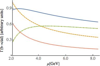
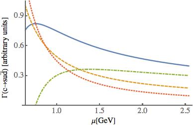
Figure 1: Scale dependence of $\Gamma(b\to cud)$ (left panel) and $\Gamma(c\to sud)$ (right panel) in the $\overline{\text{MS}}$ scheme. The solid-blue and dashed-orange lines show the result of the LO and NLO calculations, respectively. The line in dot-dashed-green shows the LO calculation to which the term with the explicit factor of $\alpha_{s}\ln(\mu)$ in the NLO decay rate is added, displaying cancellation of scale dependence to order $\alpha_{s}$. The dotted-red line shows the difference between the blue and green lines, that is, the NLO decay rate sans the term with an explicit factor of $\ln(\mu)$.

The uncertainty from omitting higher order terms in the perturbative expansion is readily estimated as order $(\alpha_{s}(\mu_{b}))^{2}\sim 4\%$ and $(\alpha_{s}(\mu_{c}))^{2}\sim 10\%$ for $\bar{b}$ and $c$ decays, respectively. This is reflected in the uncertainty introduced by the arbitrary choice of renormalization scale $\mu$ in the calculations. For example, the fractional change in the width for a fractional change in scale, $(\Delta\Gamma/\Gamma)/(\Delta\mu/\mu)$, centered at $\mu=\mu_{b}$ and $\mu=\mu_{c}$ for $\bar{b}$ and $c$ decays, respectively, is $-0.36$, $-0.20$ and $-0.11$ for the $\overline{\text{MS}}$, meson and Upsilon schemes. It is dominated in all cases by the $\mu$-dependence of hadronic decays, and among these, of $c$ decays. The scale dependence formally cancels out to order $\alpha_{s}$, so the residual dependence is of order $\alpha_{s}^{2}$. The variation with respect to $\ln(\mu)$ of the leading order is of order $\alpha_{s}$, and this is canceled exactly by the terms involving $\alpha_{s}\ln(\mu)$ at NLO. This is shown in Fig. 1 that displays the scale dependence of the NLO calculations of $\Gamma(b\to cud)$ and $\Gamma(c\to sud)$ in the $\overline{\text{MS}}$ scheme. The dashed (orange) line shows the result of the leading order calculation, displaying stronger scale dependence than the result of the NLO calculation, displayed in the solid (blue) line. The latter is the sum of the dashed-dot (green) line and the dotted (red) line. This split is intended to demonstrate the approximate cancellation of the $\mu$ dependence that comes in at LO from the Wilson coefficients and through the running mass and NLO terms with an explicit $\alpha_{s}\ln(\mu)$: this combination is shown with the dashed-dot (green) line. Both green and red line should be flat up to corrections of order $\alpha_{s}^{2}$. We can estimate the uncertainty due the scale dependence from the range of variation in the figures, about $\pm 17\%$ and $\pm 35\%$ for $\bar{b}$ and $c$ decays, respectively. Since these hadronic decays dominate the total width of the $B_{c}$, one can estimate the total uncertainty by weighing these by their relative importance to the total width, $[(0.202)17\%+(0.743)35\%]/(0.202+0.743)=31\%.$ This can be compared with the fractional change in scale, $(\Delta\Gamma/\Gamma)/(\Delta\mu/\mu)$, using $\Delta\mu/\mu\approx\Delta\ln\mu$ which gives $\Delta\Gamma/\Gamma=-0.37\ln 2=-0.26$.

Repeating this calculation for the other schemes we infer an uncertainty from order $\alpha_{s}^{2}$/scale dependence of 26%, 14% and 8% in the $\overline{\text{MS}}$, meson and Upsilon schemes.

7.2.2 Non-relativistic expansion and Non-perturbative uncertainties

Additional uncertainties are introduced by the truncation of the non-relativistic expansion. As already explained we take into account QCD corrections truncated to order $\alpha_{s}$ while carrying out the non-relativistic expansion up to relative order $v^{4}$. Since the power counting in NRQCD has $v\sim\alpha_{s}$ this is not fully consistent. However, WA and PI come in first at order $v^{6}$ and need to be retained because they are numerically important because the 2-body phase space gives an amplification by a factor of $16\pi^{2}$. Corrections to 3-body decays of relative order $v^{2}$ and $v^{4}$ are included, so their numerical effect can be estimated and analyzed. We do not include any QCD corrections to WA and PI, since they would correspond to higher-order velocity terms which we are neglecting. Furthermore, to have a fully consistent calculation at $\mathcal{O}(v^{3})$, three-loop corrections to the rate are required, consisting of three-loop corrections to the matrix elements, a three-loop matching calculation as well as four-loop running. Such corrections are however not available at present and are expected to be smaller than the WA and PI contributions, since they are not enhanced by $16\pi^{2}$ from the 2-body phase space.

Table 5 shows the fractional change in the width per fractional change in individual parameters. This table can be used to adjust the estimated partial widths in Tab. 3 by a change in the input parameters in Tab. 2. The second column in Tab. 5, “$\Delta p/p$”, gives our best guess of the fractional uncertainty in the parameter $p$, so the fractional uncertainties $\Delta\Gamma/\Gamma$ are estimated by taking the product of the second column with the entries in column 3–5. It is seen that the uncertainty introduced by the poor knowledge of the matrix elements that go into the non-relativistic expansion is $\leq 2\%$ for all entries. The reason is that, in fact, the non-relativistic corrections arising from non-perturbative matrix elements (that is, other than from the QCD-perturbative expansion of the free quark decays) are small.

We have already seen in (69) that the non-relativistic corrections are small, of order 4% for $\Gamma_{\bar{b}\to\bar{c}u(\bar{s}+\bar{d})}$. The corrections are slightly larger for the other $\bar{b}$ decay modes, up to $\sim 10\%$ for the semileptonic modes, but since the width is dominated by the hadronic modes, the non-relativistic correction to $\Gamma_{\bar{b}\to\bar{c}}$ is 4% and 5% in the $\overline{\text{MS}}$ and meson/Upsilon schemes, respectively. Similarly, we find the non-relativistic correction to $\Gamma_{c\to(s+d)}$ is 6%, 7% and 10% in the $\overline{\text{MS}}$, meson and Upsilon scheme. The small magnitude of the corrections both suggest the error from truncating the expansion is small, and the uncertainty introduced from the limited knowledge of the matrix elements is small, as expected from the previous paragraphs.

The rate of convergence of the non-relativistic expansion can also be seen by estimating the matrix element of the bilinear $\bar{Q}Q$, that enters at leading order in the OPE, expressed in terms of NRQCD fields, as given in (5.1). We find, in the Upsilon scheme, the expansion:

$$1-0.017-0.007+0.0005$$

$$1-0.180+0.014+0.051$$

where the first line is for $\bar{b}b$ and the second for $\bar{c}c$, and the first, second and third corrections correspond to the terms $\vec{D}^{2}$, $g_{s}\vec{\sigma}\cdot\vec{B}$ and $g_{s}\vec{D}\cdot\vec{E}$, and $\vec{D}^{4}$, respectively. As expected the non-relativistic expansion converges faster for $b$ quark decay than for $c$ quarks. We remind the reader that for the coefficient of the correction terms we have not included radiative corrections to the coefficient $C_{q}^{(3)}$ in the OPE; see the discussion at the end of Sec. 5.1. This truncation represents a correction $\sim 6\%$ in the $\bar{c}c$ case.

7.2.3 Parametric and numerical uncertainties

Additional uncertainties are introduced parametrically, from the uncertainty in the input parameters. The parametric uncertainty from $\alpha_{s}$ is subsumed into the scale uncertainty discussed in Sec. 7.2.1 above. Except for $|V_{cb}|$ and the non-perturbative parameters that enter the non-relativistic expansion, the input parameters in Tab. 2 have negligible uncertainties compared to those that have already been discussed. The uncertainty from $|V_{cb}|$ can be read-off Tab. 5 that gives a fractional uncertainty in $\Gamma_{B_{c}}$ slightly smaller than the fractional error in $|V_{cb}|$: $\Delta\Gamma/\Gamma\lesssim\Delta|V_{cb}|/|V_{cb}|$.

For the $\overline{\text{MS}}$ scheme there are additional parametric uncertainties from the input value of the quark masses. The resulting uncertainty is largely due to the fifth power dependence of the partial widths on the mass of the decaying quark. The conservative estimate of the uncertainty assumes that both quark masses deviate in the same direction from the central value quoted in Tab. 2. In Tab. 5 we show the result of varying $\overline{m}_{b}(\overline{m}_{b})$ and $\overline{m}_{c}(\overline{m}_{c})$ independently, and in the final result we (over)estimate the uncertainty by adding these linearly, rather than by varying them together.

Additional uncertainties are introduced in the numerical integration of various QCD corrections and the need to compute at non-zero but sufficiently small gluon mass. We have verified that the error introduce by the numerical integration and zero gluon mass extrapolation is much below a percent.

7.2.4 Strange quark mass

The non-vanishing of the strange quark mass reduces the $c$ quark decay rate, relative to the rate for $m_{s}=0$, by 7%, 7% and 6% in the $\overline{\text{MS}}$, meson and Upsilon schemes. A naive estimate of the effect of the strange mass on the $\bar{b}$-quark decay is obtained as this fraction times $(m_{c}/m_{b})^{2}\sim 0.1$ of the $\bar{b}$-quark width, or $\Delta\Gamma_{b}\lesssim 0.003\;\text{ps}^{-1}$. More dramatic is the uncertainty derived from the lesser well determined input, $\overline{m}_{s}(2\;\text{GeV})$, listed in Tab. 2. Estimating this as $\pm 10\%$ of the 6-7% reduction in the rate for $c$-quark decay, this results in an uncertainty $\Delta\Gamma_{c}\sim 0.01\;\text{ps}^{-1}$.

8 Conclusions

The result for the decay rate of the $B_{c}$ meson, displaying the contributions by decay channel and for each of the three mass schemes introduced in Sec. 2, is presented in Tab. 3 for $m_{s}=0$, and in Tab. 4 for $m_{s}\neq 0$ in decay channels involving $c$-quark decay. In Sec. 7.2 we gave a detailed accounting of uncertainties in those calculated partial widths. We summarize our results: neglecting light quark masses, including that of the strange quark, our final result for the total width of the $B_{c}$ meson in the $\overline{\text{MS}}$-, meson- and Upsilon-schemes is:

$$\Gamma^{\overline{\text{MS}}}_{B_{c}} =(1.58\pm 0.40|^{\mu}\pm 0.08|^{\text{n.p.}}\pm 0.02|^{\overline{m}}\pm 0.01|^{V_{cb}})\,\,\text{ps}^{-1}\,,$$ (70)

$$\Gamma^{\text{meson}}_{B_{c}} =(1.77\pm 0.25|^{\mu}\pm 0.20|^{\text{n.p.}}\pm 0.01|^{V_{cb}})\,\,\text{ps}^{-1}\,,$$

$$\Gamma^{\text{Upsilon}}_{B_{c}} =(2.51\pm 0.19|^{\mu}\pm 0.21|^{\text{n.p.}}\pm 0.01|^{V_{cb}})\,\,\text{ps}^{-1}\,,$$

where we indicate the uncertainties due to scale dependence ($\mu$), non-perturbative effects (n.p.), the value of $|V_{cb}|$, and for the $\overline{\text{MS}}$ scheme the input values of the masses ($\overline{m}$). As discussed above, for $m_{s}\neq 0$, the central values of the $c$-decay widths get reduced by about 7%, leading to the following total decay rates:

$$\Gamma^{\overline{\text{MS}}}_{B_{c}} =(1.51\pm 0.38|^{\mu}\pm 0.08|^{\text{n.p.}}\pm 0.02|^{\overline{m}}\pm 0.01|^{m_{s}}\pm 0.01|^{V_{cb}})\,\,\text{ps}^{-1}\,,\quad(m_{s}\neq 0)$$ (71)

$$\Gamma^{\text{meson}}_{B_{c}} =(1.70\pm 0.24|^{\mu}\pm 0.20|^{\text{n.p.}}\pm 0.01|^{m_{s}}\pm 0.01|^{V_{cb}})\,\,\text{ps}^{-1}\,,\quad(m_{s}\neq 0)$$

$$\Gamma^{\text{Upsilon}}_{B_{c}} =(2.40\pm 0.19|^{\mu}\pm 0.21|^{\text{n.p.}}\pm 0.01|^{m_{s}}\pm 0.01|^{V_{cb}})\,\,\text{ps}^{-1}\,,\quad(m_{s}\neq 0)$$

For the scale uncertainty we have used Tab. 5 with $\Delta\mu/\mu=\ln(2)$. The uncertainty due to non-perturbative effects captures the result of the non-relativistic truncation as well as the uncertainty in the matrix elements. We add linearly the absolute values of the errors from rows 4 – 9 (parameters $T$ through $f_{B_{c}}$) using for $\Delta p/p$ the values indicated on the second column, and to this we add linearly the absolute value of the estimate of a non-relativistic truncation error. The latter is estimated as a fraction, equal to the quark velocity $v_{b}\approx 0.19$ or $v_{c}\approx 0.60$, of the non-relativistic correction to the $\bar{b}$ and $c$ decays, respectively, that has been included in the partial widths recorded on Tabs. 3 and 4. Linearly adding these uncertainties is the most conservative way to proceed. Adding them instead in quadratures leads to the smaller uncertainties $\pm 0.05\,\text{ps}^{-1}$, $\pm 0.11\,\text{ps}^{-1}$ and $\pm 0.12\,\text{ps}^{-1}$ for both massless and massive strange quarks in the $\overline{\text{MS}}$, meson and Upsilon scheme, respectively.

Br(process)	$\overline{\text{MS}}$	meson	Upsilon
$b\to cu(d+s)$	13.6	15.7	11.1
$b\to cc(d+s)$	6.2	7.2	5.1
$b\to ce\nu$	3.5	3.9	2.7
$b\to c\tau\nu$	0.6	0.9	0.6
$b\to c$	27.3	31.4	22.2
$c\to su\bar{d}$	41.8	38.0	45.6
$c\to su\bar{s}$	2.1	1.9	2.4
$c\to du\bar{d}$	2.4	2.2	2.6
$c\to se\bar{\nu}$	9.4	8.4	9.2
$c\to de\bar{\nu}$	0.5	0.5	0.5
$c\to s$	66.4	60.1	70.2
$bc\to cs$	3.7	6.0	5.8
$bc\to\tau\nu$	2.6	2.5	1.8

Table 6: Branching fractions in per-cent for $B_{c}$ semi-inclusive decays in the $\overline{\text{MS}}$, meson, and Upsilon schemes. The WA into $cs$ and the PI have been combined into a single $bc\to cs$ branching fraction.

For either massless or massive strange quarks the three different schemes are consistent with each other within their respective uncertainties. The difference between the values in the meson and Upsilon scheme can mainly be traced back to the different charm mass used in the charm decays. The wide range spanned by the widths calculated in the three schemes, i.e., the strong scheme dependence, however calls for an improvement of the SM prediction. The main uncertainty, from scale dependence, can be reduced by going one order higher in the perturbative expansion, i.e., using NNLL Wilson coefficients, as well as computing the matrix elements up to two loops. While one should see convergence of the various schemes on a single value for the perturbative partial widths of the underlying $\bar{b}$ and $c$ decays as the calculation is carried out to higher order in $\alpha_{s}$, we expect the Upsilon scheme to converge fastest. Evidence for this was presented in Sec. 2.6 using the known 2-loop results for the semileptonic decays of $b$ and $c$ quarks. This is also substantiated by the milder scale dependence of the result in the Upsilon scheme compared to the other schemes. The non-perturbative uncertainty is dominated by our estimate of the order $v^{3}$ corrections. These arise solely from order $\alpha_{s}$ corrections to the Wilson coefficients of order $v^{2}$ operators. Additional perturbative corrections to Wilson coefficients will have a marginal effect on the overall precision. More precise determinations of the relevant non-perturbative parameters (for example from lattice QCD) might however become important in the future.

It is interesting to note that branching fractions predicted by the three schemes are in good agreement with each other, as shown in Tab. 6. This may be interpreted as evidence that the dominant factor in the differences between scheme predictions is from the sensitive dependence on masses of the $\bar{b}$ and $c$ quarks, which differ vastly among the schemes. We have not attempted to estimate uncertainties in the branching fractions, which however are expected to be significantly smaller in the ratios than in the individual partial widths because of cancellation of correlated uncertainties.

Previous calculations of the lifetime of $B_{c}$ mesons yield results closer to the experimental measured value than we present here. However, the total width depends sensitively on the choice of masses for the $b$ and $c$ quarks. An arbitrary choice can be made to yield a result close to the experimental value. We have, instead, computed systematically, eliminating the pole mass in favour of well defined masses and truncating the perturbative expansion consistently. This guarantees cancellation of renormalon ambiguities, that remain present if calculating in terms of ad hoc values for the on-shell masses. We find it is interesting to note that the Upsilon scheme results have at once the smallest uncertainty and give partial widths that are seemingly too large. In particular the semileptonic partial width $\Gamma_{c\to(s+d)e\nu}$ is much larger than in both the two other schemes and the result of BB. However, as we have remarked earlier, it is this higher value that gives excellent agreement with the decay width for inclusive semileptonic decays of $D$ mesons. Similarly, the Upsilon and meson schemes give excellent agreement with the inclusive width for semileptonic $B$ meson decay.

The calculations presented depend on the assumption that quark-hadron duality validates the OPE method. Similarly, for the Upsilon scheme, and to lesser extend for the meson scheme, the nonperturbative contribution to the pole masses have been neglected. These assumptions need to be validated through other means. Were the predictions to fail the conclusion could well be that one or both of these assumptions are not valid.

Finally, the initial motivation for this computation, namely to distinguish NP contributions in the $B_{c}$ life-time remains challenging, and further progress on the theory side has to be made before clear-cut conclusions concerning new-physics effects in $\Gamma_{B_{c}}$ can be drawn.

Acknowledgments — We thank Christine Davies and Aneesh Manohar for useful discussions. J. A. acknowledges financial support from the Swiss National Science Foundation (Project No.P400P2_183838). The work of B.G. is supported in part by the U.S. Department of Energy Grant No. DE-SC0009919.

References

- [1] LHCb Collaboration, R. Aaij et al., Measurement of the meson lifetime using decays, Eur. Phys. J. C 74 (2014), no. 5 2839, [arXiv:1401.6932].
- [2] LHCb Collaboration, R. Aaij et al., Measurement of the lifetime of the meson using the decay mode, Phys. Lett. B 742 (2015) 29–37, [arXiv:1411.6899].
- [3] CMS Collaboration, A. M. Sirunyan et al., Measurement of b hadron lifetimes in pp collisions at 8 TeV, Eur. Phys. J. C 78 (2018), no. 6 457, [arXiv:1710.08949]. [Erratum: Eur.Phys.J.C 78, 561 (2018)].
- [4] Particle Data Group Collaboration, K. Olive et al., Review of Particle Physics, Chin. Phys. C 38 (2014) 090001.
- [5] I. I. Bigi, Inclusive B(c) decays as a QCD lab, Phys. Lett. B 371 (1996) 105–110, [hep-ph/9510325].
- [6] M. Beneke and G. Buchalla, The Meson Lifetime, Phys. Rev. D 53 (1996) 4991–5000, [hep-ph/9601249].
- [7] C.-H. Chang, S.-L. Chen, T.-F. Feng, and X.-Q. Li, The Lifetime of meson and some relevant problems, Phys. Rev. D 64 (2001) 014003, [hep-ph/0007162].
- [8] V. Kiselev, A. Kovalsky, and A. Likhoded, decays and lifetime in QCD sum rules, Nucl. Phys. B 585 (2000) 353–382, [hep-ph/0002127].
- [9] S. Gershtein, V. Kiselev, A. Likhoded, and A. Tkabladze, Physics of B(c) mesons, Phys. Usp. 38 (1995) 1–37, [hep-ph/9504319].
- [10] I. Gouz, V. Kiselev, A. Likhoded, V. Romanovsky, and O. Yushchenko, Prospects for the studies at LHCb, Phys. Atom. Nucl. 67 (2004) 1559–1570, [hep-ph/0211432].
- [11] BaBar Collaboration, J. Lees et al., Evidence for an excess of decays, Phys. Rev. Lett. 109 (2012) 101802, [arXiv:1205.5442].
- [12] BaBar Collaboration, J. Lees et al., Measurement of an Excess of Decays and Implications for Charged Higgs Bosons, Phys. Rev. D 88 (2013), no. 7 072012, [arXiv:1303.0571].
- [13] Belle Collaboration, M. Huschle et al., Measurement of the branching ratio of relative to decays with hadronic tagging at Belle, Phys. Rev. D 92 (2015), no. 7 072014, [arXiv:1507.03233].
- [14] Belle Collaboration, Y. Sato et al., Measurement of the branching ratio of relative to decays with a semileptonic tagging method, Phys. Rev. D 94 (2016), no. 7 072007, [arXiv:1607.07923].
- [15] LHCb Collaboration, R. Aaij et al., Measurement of the ratio of branching fractions , Phys. Rev. Lett. 115 (2015), no. 11 111803, [arXiv:1506.08614]. [Erratum: Phys.Rev.Lett. 115, 159901 (2015)].
- [16] Belle Collaboration, S. Hirose et al., Measurement of the lepton polarization and in the decay , Phys. Rev. Lett. 118 (2017), no. 21 211801, [arXiv:1612.00529].
- [17] LHCb Collaboration, R. Aaij et al., Measurement of the ratio of branching fractions /, Phys. Rev. Lett. 120 (2018), no. 12 121801, [arXiv:1711.05623].
- [18] X.-Q. Li, Y.-D. Yang, and X. Zhang, Revisiting the one leptoquark solution to the ) anomalies and its phenomenological implications, JHEP 08 (2016) 054, [arXiv:1605.09308].
- [19] R. Alonso, B. Grinstein, and J. Martin Camalich, Lifetime of Constrains Explanations for Anomalies in , Phys. Rev. Lett. 118 (2017), no. 8 081802, [arXiv:1611.06676].
- [20] G. Branco, P. Ferreira, L. Lavoura, M. Rebelo, M. Sher, and J. P. Silva, Theory and phenomenology of two-Higgs-doublet models, Phys. Rept. 516 (2012) 1–102, [arXiv:1106.0034].
- [21] A. Crivellin, C. Greub, and A. Kokulu, Explaining , and in a 2HDM of type III, Phys. Rev. D 86 (2012) 054014, [arXiv:1206.2634].
- [22] A. Crivellin, A. Kokulu, and C. Greub, Flavor-phenomenology of two-Higgs-doublet models with generic Yukawa structure, Phys. Rev. D 87 (2013), no. 9 094031, [arXiv:1303.5877].
- [23] J. M. Cline, Scalar doublet models confront and b anomalies, Phys. Rev. D 93 (2016), no. 7 075017, [arXiv:1512.02210].
- [24] C. Kim, Y. W. Yoon, and X.-B. Yuan, Exploring top quark FCNC within 2HDM type III in association with flavor physics, JHEP 12 (2015) 038, [arXiv:1509.00491].
- [25] A. Crivellin, J. Heeck, and P. Stoffer, A perturbed lepton-specific two-Higgs-doublet model facing experimental hints for physics beyond the Standard Model, Phys. Rev. Lett. 116 (2016), no. 8 081801, [arXiv:1507.07567].
- [26] L. Wang, J. M. Yang, and Y. Zhang, Probing a pseudoscalar at the LHC in light of and muon g-2 excesses, Nucl. Phys. B 924 (2017) 47–62, [arXiv:1610.05681].
- [27] W.-S. Hou, Enhanced charged Higgs boson effects in and , Phys. Rev. D 48 (1993) 2342–2344.
- [28] M. Tanaka, Charged Higgs effects on exclusive semitauonic decays, Z. Phys. C 67 (1995) 321–326, [hep-ph/9411405].
- [29] K. Kiers and A. Soni, Improving constraints on using , Phys. Rev. D 56 (1997) 5786–5793, [hep-ph/9706337].
- [30] C.-H. Chen and C.-Q. Geng, Charged Higgs on and , JHEP 10 (2006) 053, [hep-ph/0608166].
- [31] R. Alonso, B. Grinstein, and J. Martin Camalich, Lepton universality violation and lepton flavor conservation in -meson decays, JHEP 10 (2015) 184, [arXiv:1505.05164].
- [32] A. H. Hoang, Z. Ligeti, and A. V. Manohar, B decay and the Upsilon mass, Phys. Rev. Lett. 82 (1999) 277–280, [hep-ph/9809423].
- [33] A. H. Hoang, Z. Ligeti, and A. V. Manohar, B decays in the upsilon expansion, Phys. Rev. D 59 (1999) 074017, [hep-ph/9811239].
- [34] E. Bagan, P. Ball, V. M. Braun, and P. Gosdzinsky, Charm quark mass dependence of QCD corrections to nonleptonic inclusive decays, Nucl. Phys. B 432 (1994) 3–38, [hep-ph/9408306].
- [35] E. Bagan, P. Ball, V. M. Braun, and P. Gosdzinsky, Theoretical update of the semileptonic branching ratio of mesons, Phys. Lett. B 342 (1995) 362–368, [hep-ph/9409440]. [Erratum: Phys.Lett.B 374, 363–364 (1996)].
- [36] F. Krinner, A. Lenz, and T. Rauh, The inclusive decay revisited, Nucl. Phys. B 876 (2013) 31–54, [arXiv:1305.5390].
- [37] C. McNeile, C. Davies, E. Follana, K. Hornbostel, and G. Lepage, High-Precision c and b Masses, and QCD Coupling from Current-Current Correlators in Lattice and Continuum QCD, Phys. Rev. D 82 (2010) 034512, [arXiv:1004.4285].
- [38] M. Beneke, V. M. Braun, and V. I. Zakharov, Bloch-Nordsieck cancellations beyond logarithms in heavy particle decays, Phys. Rev. Lett. 73 (1994) 3058–3061, [hep-ph/9405304].
- [39] M. E. Luke, A. V. Manohar, and M. J. Savage, Renormalons in effective field theories, Phys. Rev. D 51 (1995) 4924–4933, [hep-ph/9407407].
- [40] M. Neubert and C. T. Sachrajda, Cancellation of renormalon ambiguities in the heavy quark effective theory, Nucl. Phys. B 438 (1995) 235–260, [hep-ph/9407394].
- [41] A. Sinkovics, R. Akhoury, and V. I. Zakharov, Cancellation of corrections to the inclusive decay width of a heavy quark, Phys. Rev. D 58 (1998) 114025, [hep-ph/9804401].
- [42] N. Gray, D. J. Broadhurst, W. Grafe, and K. Schilcher, Three Loop Relation of Quark (Modified) Ms and Pole Masses, Z. Phys. C 48 (1990) 673–680.
- [43] P. Marquard, L. Mihaila, J. Piclum, and M. Steinhauser, Relation between the pole and the minimally subtracted mass in dimensional regularization and dimensional reduction to three-loop order, Nucl. Phys. B 773 (2007) 1–18, [hep-ph/0702185].
- [44] J. Chay, H. Georgi, and B. Grinstein, Lepton energy distributions in heavy meson decays from QCD, Phys. Lett. B 247 (1990) 399–405.
- [45] A. Pineda and F. Yndurain, Calculation of quarkonium spectrum and , to order , Phys. Rev. D 58 (1998) 094022, [hep-ph/9711287].
- [46] K. Melnikov and A. Yelkhovsky, The quark low scale running mass from Upsilon sum rules, Phys. Rev. D 59 (1999) 114009, [hep-ph/9805270].
- [47] A. Hoang, M. Smith, T. Stelzer, and S. Willenbrock, Quarkonia and the pole mass, Phys. Rev. D 59 (1999) 114014, [hep-ph/9804227].
- [48] M. Beneke, A Quark mass definition adequate for threshold problems, Phys. Lett. B 434 (1998) 115–125, [hep-ph/9804241].
- [49] A. V. Manohar and M. B. Wise, Heavy quark physics. Cambridge University Press, 2000.
- [50] K. G. Chetyrkin, J. H. Kuhn, and M. Steinhauser, RunDec: A Mathematica package for running and decoupling of the strong coupling and quark masses, Comput. Phys. Commun. 133 (2000) 43–65, [hep-ph/0004189].
- [51] H. Leutwyler, How to Use Heavy Quarks to Probe the QCD Vacuum, Phys. Lett. B 98 (1981) 447–450.
- [52] M. Voloshin, Precoulombic Asymptotics for Energy Levels of Heavy Quarkonium, Sov. J. Nucl. Phys. 36 (1982) 143.
- [53] A. Pak and A. Czarnecki, Heavy-to-heavy quark decays at NNLO, Phys. Rev. D 78 (2008) 114015, [arXiv:0808.3509].
- [54] K. Melnikov, corrections to semileptonic decay , Phys. Lett. B 666 (2008) 336–339, [arXiv:0803.0951].
- [55] A. J. Buras, Weak Hamiltonian, CP violation and rare decays, in Les Houches Summer School in Theoretical Physics, Session 68: Probing the Standard Model of Particle Interactions, pp. 281–539, 6, 1998. hep-ph/9806471.
- [56] A. Buras, Gauge Theories of Weak Decays. Cambridge University Press, 6, 2020.
- [57] J. Aebischer, M. Fael, C. Greub, and J. Virto, B physics Beyond the Standard Model at One Loop: Complete Renormalization Group Evolution below the Electroweak Scale, JHEP 09 (2017) 158, [arXiv:1704.06639].
- [58] G. Lepage, L. Magnea, C. Nakhleh, U. Magnea, and K. Hornbostel, Improved nonrelativistic QCD for heavy quark physics, Phys. Rev. D 46 (1992) 4052–4067, [hep-lat/9205007].
- [59] B. Grinstein and I. Z. Rothstein, Effective field theory and matching in nonrelativistic gauge theories, Phys. Rev. D 57 (1998) 78–82, [hep-ph/9703298].
- [60] A. V. Manohar, Heavy quark effective theory and nonrelativistic QCD Lagrangian to order , Phys. Rev. D 56 (1997) 230–237, [hep-ph/9701294].
- [61] H. Dahmen, B. Scholz, and F. Steiner, Infrared Dynamics of Quantum Electrodynamics and the Asymptotic Behavior of the Electron Form-factor, Nucl. Phys. B 202 (1982) 365–381.
- [62] B. Guberina, R. Peccei, and R. Ruckl, Weak Decays of Heavy Quarks, Phys. Lett. B 91 (1980) 116–120.
- [63] G. Altarelli, G. Curci, G. Martinelli, and S. Petrarca, QCD Nonleading Corrections to Weak Decays as an Application of Regularization by Dimensional Reduction, Nucl. Phys. B 187 (1981) 461–513.
- [64] G. Altarelli and S. Petrarca, Inclusive beauty decays and the spectator model, Phys. Lett. B 261 (1991) 303–310.
- [65] G. Buchalla, QCD corrections to charm quark decay in dimensional regularization with non-anticommuting , Nucl. Phys. B 391 (1993) 501–514.
- [66] Q. Hokim and X.-Y. Pham, Exact one-gluon corrections for inclusive weak processes, Annals of Physics 155 (1984), no. 1 202 – 227.
- [67] N. Cabibbo and L. Maiani, The Lifetime of Charmed Particles, Phys. Lett. B 79 (1978) 109–111.
- [68] Y. Nir, The Mass Ratio in Semileptonic Decays, Phys. Lett. B 221 (1989) 184–190.
- [69] M. E. Luke and A. V. Manohar, Reparametrization invariance constraints on heavy particle effective field theories, Phys. Lett. B 286 (1992) 348–354, [hep-ph/9205228].
- [70] E. Bagan, P. Ball, B. Fiol, and P. Gosdzinsky, Next-to-leading order radiative corrections to the decay , Phys. Lett. B 351 (1995) 546–554, [hep-ph/9502338].
- [71] M. Neubert and C. T. Sachrajda, Spectator effects in inclusive decays of beauty hadrons, Nucl. Phys. B 483 (1997) 339–370, [hep-ph/9603202].
- [72] S. Gershtein, V. Kiselev, A. Likhoded, and A. Tkabladze, spectroscopy, Phys. Rev. D 51 (1995) 3613–3627, [hep-ph/9406339].
- [73] Fermilab Lattice, MILC, TUMQCD Collaboration, A. Bazavov et al., Up-, down-, strange-, charm-, and bottom-quark masses from four-flavor lattice QCD, Phys. Rev. D 98 (2018), no. 5 054517, [arXiv:1802.04248].
- [74] B. Colquhoun, R. J. Dowdall, C. T. H. Davies, K. Hornbostel, and G. P. Lepage, and Leptonic Widths, and from full lattice QCD, Phys. Rev. D 91 (2015), no. 7 074514, [arXiv:1408.5768].
- [75] HPQCD Collaboration, A. T. Lytle, C. T. H. Davies, D. Hatton, G. P. Lepage, and C. Sturm, Determination of quark masses from lattice QCD and the RI-SMOM intermediate scheme, Phys. Rev. D 98 (2018), no. 1 014513, [arXiv:1805.06225].
- [76] Particle Data Group Collaboration, M. Tanabashi et al., Review of Particle Physics, Phys. Rev. D 98 (2018), no. 3 030001.
- [77] C. McNeile, C. Davies, E. Follana, K. Hornbostel, and G. Lepage, Heavy meson masses and decay constants from relativistic heavy quarks in full lattice QCD, Phys. Rev. D 86 (2012) 074503, [arXiv:1207.0994].
- [78] R. Dowdall, C. Davies, T. Hammant, and R. Horgan, Precise heavy-light meson masses and hyperfine splittings from lattice QCD including charm quarks in the sea, Phys. Rev. D 86 (2012) 094510, [arXiv:1207.5149].