Computing the $4$-Edge-Connected Components of a Graph in Linear Time

Abstract

We present the first linear-time algorithm that computes the $4$-edge-connected components of an undirected graph. Hence, we also obtain the first linear-time algorithm for testing $4$-edge connectivity. Our results are based on a linear-time algorithm that computes the $3$-edge cuts of a $3$-edge-connected graph $G$, and a linear-time procedure that, given the collection of all $3$-edge cuts, partitions the vertices of $G$ into the $4$-edge-connected components.

1 Introduction

Let $G=(V,E)$ be a connected undirected graph with $m$ edges and $n$ vertices. An (edge) cut of $G$ is a set of edges $S\subseteq E$ such that $G\setminus S$ is not connected. We say that $S$ is a $k$-cut if its cardinality is $|S|=k$. Also, we refer to the $1$-cuts as the bridges of $G$. A cut $S$ is minimal if no proper subset of $S$ is a cut of $G$. The edge connectivity of $G$, denoted by $\lambda(G)$, is the minimum cardinality of an edge cut of $G$. A graph is $k$-edge-connected if $\lambda(G)\geq k$.

A cut $S$ separates two vertices $u$ and $v$, if $u$ and $v$ lie in different connected components of $G\setminus S$. Vertices $u$ and $v$ are $k$-edge-connected, denoted by $u\stackrel{{\scriptstyle[}}{{]}}{G}{\equiv}_{k}v$, if there is no $(k-1)$-cut that separates them. By Menger’s theorem [15], $u$ and $v$ are $k$-edge-connected if and only if there are $k$-edge-disjoint paths between $u$ and $v$. A $k$-edge-connected component of $G$ is a maximal set $C\subseteq V$ such that there is no $(k-1)$-edge cut in $G$ that disconnects any two vertices $u,v\in C$ (i.e., $u$ and $v$ are in the same connected component of $G\setminus S$ for any $(k-1)$-edge cut $S$). We can define, analogously, the vertex cuts and the $k$-vertex-connected components of $G$.

Computing and testing the edge connectivity of a graph, as well as its $k$-edge-connected components, is a classical subject in graph theory, as it is an important notion in several application areas (see, e.g., [17]), that has been extensively studied since the 1970’s. It is known how to compute the $(k-1)$-edge cuts, $(k-1)$-vertex cuts, $k$-edge-connected components and $k$-vertex-connected components of a graph in linear time for $k\in\{2,3\}$ [5, 9, 16, 19, 22]. The case $k=4$ has also received significant attention [2, 3, 10, 11]. Unfortunately, none of the previous algorithms achieved linear running time. In particular, Kanevsky and Ramachandran [10] showed how to test whether a graph is $4$-vertex-connected in $O(n^{2})$ time. Furthermore, Kanevsky et al. [11] gave an $O(m+n\alpha(m,n))$-time algorithm to compute the $4$-vertex-connected components of a $3$-vertex-connected graph, where $\alpha$ is a functional inverse of Ackermann’s function [21]. Using the reduction of Galil and Italiano [5] from edge connectivity to vertex connectivity, the same bounds can be obtained for $4$-edge connectivity. Specifically, one can test whether a graph is $4$-edge-connected in $O(n^{2})$ time, and one can compute the $4$-edge-connected components of a $3$-edge-connected graph in $O(m+n\alpha(m,n))$ time. Dinitz and Westbrook [3] presented an $O(m+n\log{n})$-time algorithm to compute the $4$-edge-connected components of a general graph $G$ (i.e., when $G$ is not necessarily $3$-edge-connected). Nagamochi and Watanabe [18] gave an $O(m+k^{2}n^{2})$-time algorithm to compute the $k$-edge-connected components of a graph $G$, for any integer $k$. We also note that the edge connectivity of a simple undirected graph can be computed in ${O}(m\mathrm{polylog}{n})$ time, randomized [7, 12] or deterministic [8, 14]. The best current bound is $O(m\log^{2}{n}\log{\log}^{2}{n})$, achieved by Henzinger et al. [8] which provided an improved version of the algorithm of Kawarabayashi and Thorup [14].

Our results and techniques

In this paper we present the first linear-time algorithm that computes the $4$-edge-connected components of a general graph $G$, thus resolving a problem that remained open for more than 20 years. Hence, this also implies the first linear-time algorithm for testing $4$-edge connectivity. We base our results on the following ideas. First, we extend the framework of Georgiadis and Kosinas [6] for computing $2$-edge cuts (as well as mixed cuts consisting of a single vertex and a single edge) of $G$. Similar to known linear-time algorithms for computing $3$-vertex-connected and $3$-edge-connected components [9, 22], Georgiadis and Kosinas [6] define various concepts with respect to a depth-first search (DFS) spanning tree of $G$. We extend this framework by introducing new key parameters that can be computed efficiently and provide characterizations of the various types of $3$-edge cuts that may appear in a $3$-edge-connected graph. We deal with the general case by dividing $G$ into auxiliary graphs $H_{1},\ldots,H_{\ell}$, such that each $H_{i}$ is $3$-edge-connected and corresponds to a different $3$-edge-connected component of $G$. Also, for any two vertices $x$ and $y$, we have $x\stackrel{{\scriptstyle[}}{{]}}{G}{\equiv}_{4}y$ if and only if $x$ and $y$ are both in the same auxiliary graph $H_{i}$ and $x\stackrel{{\scriptstyle[}}{{]}}{H_{i}}{\equiv}_{4}y$. Furthermore, this reduction allows us to compute in linear time the number of minimal $3$-edge cuts in a general graph $G$. Next, in order to compute the $4$-edge-connected components in each auxiliary graph $H_{i}$, we utilize the fact that a minimum cut of a graph $G$ separates $G$ into two connected components. Hence, we can define the set $V_{C}$ of the vertices in the connected component of $G\setminus{C}$ that does not contain a specified root vertex $r$. We refer to the number of vertices in $V_{C}$ as the $r$-size of the cut $C$. Then, we apply a recursive algorithm that successively splits $H_{i}$ into smaller graphs according to its $3$-cuts. When no more splits are possible, the connected components of the final split graph correspond to the $4$-edge-connected components of $G$. We show that we can implement this procedure in linear time by processing the cuts in non-decreasing order with respect to their $r$-size.

2 Concepts defined on a DFS-tree structure

Let $G=(V,E)$ be a connected undirected graph, which may have multiple edges. For a set of vertices $S\subseteq V$, the induced subgraph of $S$, denoted by $G[S]$, is the subgraph of $G$ with vertex set $S$ and edge set $\{e\in E\mid$ both ends of $e$ lie in $S\}$. Let $T$ be the spanning tree of $G$ provided by a depth-first search (DFS) of $G$ [19], with start vertex $r$. The edges in $T$ are called tree-edges; the edges in $E\setminus T$ are called back-edges, as their endpoints have ancestor-descendant relation in $T$. A vertex $u$ is an ancestor of a vertex $v$ ($v$ is a descendant of $u$) if the tree path from $r$ to $v$ contains $u$. Thus, we consider a vertex to be an ancestor (and, consequently, a descendant) of itself. We let $p(v)$ denote the parent of a vertex $v$ in $T$. If $u$ is a descendant of $v$ in $T$, we denote the set of vertices of the simple tree path from $u$ to $v$ as $\mathit{T}[u,v]$. The expressions $\mathit{T}[u,v)$ and $\mathit{T}(u,v]$ have the obvious meaning (i.e., the vertex on the side of the parenthesis is excluded). From now on, we identify vertices with their preorder number (assigned during the DFS). Thus, $v$ being an ancestor of $u$ in $T$ implies that $v\leq u$. Let $T(v)$ denote the set of descendants of $v$, and let $\mathit{ND}(v)$ denote the number of descendants of $v$ (i.e. $\mathit{ND}(v)=|T(v)|$). With all $\mathit{ND}(v)$ computed, we can check in constant time whether a vertex $u$ is a descendant of $v$, since $u\in T(v)$ if and only if $v\leq u$ and $u<v+\mathit{ND}(v)$ [20].

Whenever $(x,y)$ denotes a back-edge, we shall assume that $x$ is a descendant of $y$. We let $B(v)$ denote the set of back-edges $(x,y)$, where $x$ is a descendant of $v$ and $y$ is a proper ancestor of $v$. Thus, if we remove the tree-edge $(v,p(v))$, $T(v)$ remains connected to the rest of the graph through the back-edges in $B(v)$. This implies that $G$ is $2$-edge-connected if and only if $|B(v)|>0$, for every $v\neq r$. Furthermore, $G$ is $3$-edge-connected only if $|B(v)|>1$, for every $v\neq r$. We let $\mathit{b\_count}(v)$ denote the number of elements of $B(v)$ (i.e. $\mathit{b\_count}(v)=|B(v)|$). $\mathit{low}(v)$ denotes the lowest $y$ such that there exists a back-edge $(x,y)\in B(v)$. Similarly, $\mathit{high}(v)$ is the highest $y$ such that there exists a back-edge $(x,y)\in B(v)$.

We let $M(v)$ denote the nearest common ancestor of all $x$ for which there exists a back-edge $(x,y)\in B(v)$. Note that $M(v)$ is a descendant of $v$. Let $m$ be a vertex and $v_{1},\dotsc,v_{k}$ be all the vertices with $M(v_{1})=\dotsc=M(v_{k})=m$, sorted in decreasing order. (Observe that $v_{i+1}$ is an ancestor of $v_{i}$, for every $i\in\{1,\dotsc,k-1\}$, since $m$ is a common descendant of all $v_{1},\dotsc,v_{k}$.) Then we have $M^{-1}(m)=\{v_{1},\dotsc,v_{k}\}$, and we define $\mathit{nextM}(v_{i})$ $:=$ $v_{i+1}$, for every $i\in\{1,\dotsc,k-1\}$, and $\mathit{lastM}(v_{i})$ $:=$ $v_{k}$, for every $i\in\{1,\dotsc,k\}$. Thus, for every vertex $v$, $\mathit{nextM}(v)$ is the successor of $v$ in the decreasingly sorted list $M^{-1}(M(v))$, and $\mathit{lastM}(v)$ is the lowest element in $M^{-1}(M(v))$.

The following two simple facts have been proved in [6].

Fact 2.1.

All $\mathit{ND}(v)$, $\mathit{b\_count}(v)$, $M(v)$, $\mathit{low}(v)$ and $\mathit{high}(v)$ can be computed in total linear-time, for all vertices $v$.

Fact 2.2.

$B(u)=B(v)$ $\Leftrightarrow$ $M(u)=M(v)$, and $\mathit{high}(u)=\mathit{high}(v)$ $\Leftrightarrow$ $M(u)=M(v)$ and $\mathit{b\_count}(u)=\mathit{b\_count}(v)$.

Furthermore, [6] implies the following characterization of a $3$-edge-connected graph.

Fact 2.3.

$G$ is $3$-edge-connected if and only if $|B(v)|>1$, for every $v\neq r$, and $B(v)\neq B(u)$, for every pair of vertices $u$ and $v$, $u\not=v$.

Lemma 2.4.

Let $v$ be an ancestor of $u$ and $M(v)$ a descendant of $u$. Then, $M(v)$ is a descendant of $M(u)$.

Proof.

Let $(x,y)\in B(v)$. Then $x$ is a descendant of $M(v)$, and therefore a descendant of $u$. Furthermore, $y$ is a proper ancestor of $v$, and therefore a proper ancestor of $u$. This shows that $(x,y)\in B(u)$, and thus we have $B(v)\subseteq B(u)$. This shows that $M(v)$ is a descendant of $M(u)$. ∎

The following lemma will be implicitly evoked several times in the following sections.

Lemma 2.5.

Let $u$ be a proper descendant of $v$ such that $M(u)=M(v)$. Then, $B(v)\subseteq B(u)$. Furthermore, if the graph is $3$-edge-connected, $B(v)\subset B(u)$.

Proof.

Let $(x,y)\in B(v)$. Then $x$ is a descendant of $M(v)$, and therefore a descendant of $M(u)$, and therefore a descendant of $u$. Furthermore, $y$ is a proper ancestor of $v$, and therefore a proper ancestor of $u$. This shows that $(x,y)\in B(u)$, and thus $B(v)\subseteq B(u)$ is established. If the graph is $3$-edge-connected, $B(v)\subset B(u)$ is an immediate consequence of fact 2.3. ∎

Now let us provide some extensions of those concepts that will be needed for our purposes. Assume that $G$ is $3$-edge-connected, and let $v\neq r$ be a vertex of $G$. By fact 2.3, $\mathit{b\_count}(v)>1$, and therefore there are at least two back-edges in $B(v)$. Of course, there is at least one back-edge $(x,y)\in B(v)$ such that $y=\mathit{low}(v)$. We let $\mathit{low1}(v)$ denote $y$, and $\mathit{low1D}(v)$ denote $x$. That is, $\mathit{low1}(v)$ is the $\mathit{low}$ point of $v$, and $\mathit{low1D}(v)$ is a descendant of $v$ which is connected with a back-edge to its $\mathit{low}$ point. (Of course, $\mathit{low1D}(v)$ is not uniquely determined, but we need to have at least one such descendant stored in a variable.) Similarly, we let $\mathit{highD}(v)$ denote a descendant of $v$ which is connected with a back-edge to the $\mathit{high}$ point of $v$. (Again, $\mathit{highD}(v)$ is not uniquely determined.) Then, there may exist another back-edge $(x^{\prime},y^{\prime})\in B(v)$ with $x^{\prime}\neq x$ and $y^{\prime}=y$. In this case, we let $\mathit{low2}(v)$ denote $y^{\prime}$ (that is, $\mathit{low2}(v)$ is, again, the $\mathit{low}$ point of $v$) and $\mathit{low2D}(v)$ denote $x^{\prime}$. If there is no back-edge $(x^{\prime},y^{\prime})\in B(v)$ with $x^{\prime}\neq x$ and $y^{\prime}=y$, let $(x^{\prime},y^{\prime})\in B(v)$ denote a back-edge with $y^{\prime}=\mathit{min}(\{w\mid\exists(z,w)\in B(v)\}\setminus\{y\})$. Then we let $\mathit{low2}(v)$ denote $y^{\prime}$ and $\mathit{low2D}(v)$ denote $x^{\prime}$. Thus, if $v\neq r$, we know that $(\mathit{low1D}(v),\mathit{low}(v))$ and $(\mathit{low2D}(v),\mathit{low2}(v))$ are two distinct back-edges in $B(v)$. We have defined $\mathit{low1}$, $\mathit{low1D}$, $\mathit{low2}$ and $\mathit{low2D}$ because we need to have stored, for every vertex $v\neq r$, two back-edges from $B(v)$ (see section 3.1). Any other pair of back-edges from $B(v)$ could do as well. It is easy to compute all $\mathit{low1}(v)$, $\mathit{low1D}(v)$, $\mathit{low2}(v)$ and $\mathit{low2D}(v)$ during the DFS.

We let $l(v)$ denote the lowest $y$ for which there exists a back-edge $(v,y)$, or $v$ if no such back-edge exists. Thus, $\mathit{low}(v)\leq l(v)$. Now let $c_{1},\dotsc,c_{k}$ be the children of $v$ sorted in non-decreasing order w.r.t. their $\mathit{low}$ point. Then we call $c_{1}$ the $\mathit{low1}$ child of $v$, and $c_{2}$ the $\mathit{low2}$ child of $v$. (Of course, the $\mathit{low1}$ and $\mathit{low2}$ children of $v$ are not uniquely determined after a DFS on $G$, since we may have $\mathit{low}(c_{1})=\mathit{low}(c_{2})$.) We let $\tilde{M}(v)$ denote the nearest common ancestor of all $x$ for which there exists a back-edge $(x,y)\in B(v)$ with $x$ a proper descendant of $M(v)$. Formally, $\tilde{M}(v)$ $:=$ nca$\{x\mid\exists(x,y)\in B(v)\mbox{ and }x\neq M(v)\}$. If the set $\{x\mid\exists(x,y)\in B(v)\mbox{ and }x\neq M(v)\}$ is empty, we leave $\tilde{M}(v)$ undefined. We also define $M_{low1}(v)$ as the nearest common ancestor of all $x$ for which there exists a back-edge $(x,y)\in B(v)$ with $x$ being a descendant of the $\mathit{low1}$ child of $M(v)$, and $M_{low2}(v)$ as the nearest common ancestor of all $x$ for which there exists a back-edge $(x,y)\in B(v)$ with $x$ a descendant of the $\mathit{low2}$ child of $M(v)$. Formally, $M_{low1}(v)$ $:=$ nca$\{x\mid\exists(x,y)\in B(v)\mbox{ and }x\mbox{ is a descendant of the }\mathit{low1}\mbox{ child of }M(v)\}$ and $M_{low2}(v)$ $:=$ nca$\{x\mid\exists(x,y)\in B(v)\mbox{ and }x\mbox{ is a descendant of the }\mathit{low2}\mbox{ child of }M(v)\}$. If the set in the formal definition of $M_{low1}(v)$ (resp. $M_{low2}(v)$) is empty, we leave $M_{low1}(v)$ (resp. $M_{low2}(v)$) undefined.

2.1 Computing the DFS parameters in linear time

Algorithm 1 shows how we can easily compute $\mathit{highD}(v)$ during the computation of all $\mathit{high}$ points. The algorithm uses the static tree disjoint-set-union data structure of Gabow and Tarjan [4] to achieve linear running time.

1 initialize a DSU structure on the vertices of $G$, where the $\mathit{link}$ operations are predetermined by the edges of $T$

2 for $v=n$ to $v=1$ do

3       foreach $u$ adjacent to $v$ do

4             if $u$ is a descendant of $v$ then

5                   $x\leftarrow\mathit{find}(u)$

6                   while $x>v$ do

7                         $\mathit{high}[x]\leftarrow v$

8                         $\mathit{highD}[x]\leftarrow u$

9                         $\mathit{next}\leftarrow\mathit{find}(p(x))$

10                         $\mathit{link}(x,p(x))$

11                         $x\leftarrow\mathit{next}$

12                   end while

13                  

14             end if

15            

16       end foreach

17      

18 end for

Algorithm 1 Compute all $\mathit{high}(v)$ and $\mathit{highD}(v)$, for all vertices $v\neq r$

Algorithm 2 shows how we can compute all $M(v)$ and $\mathit{nextM}(v)$, algorithm 3 shows how we can compute all $\tilde{M}(v)$, and algorithm 4 shows how we can compute all $M_{low1}(v)$ and $M_{low2}(v)$, for all vertices $v\neq r$, in total linear time. These algorithms process the vertices in a bottom-up fashion, and they work recursively on the descendants of a vertex. To perform these computations in linear time, we have to avoid descending to the same vertices an excessive amount of times during the recursion. To achieve this, we use a variable $\mathit{currentM}[w]$, that has the property that, during the course of the algorithm, when we process a vertex $v$, all back-edges that start from a descendant of $w$ and end in a proper ancestor of $v$ have their higher end in $T(\mathit{currentM}[w])$ (this means, of course, that $\mathit{currentM}[w]$ is a descendant of $w$). And so, if we want e.g. to compute $M_{low1}(v)$, we may descend immediately to $\mathit{currentM}[c_{1}]$, where $c_{1}$ is the $\mathit{low1}$ child of $M(v)$. In Lemma 2.7, we give a formal proof of the correctness and linear complexity of Algorithms 3 and 4.

1

// Compute all $M(v)$ and $\mathit{nextM}(v)$

2 for $v=n$ to $v=2$ do

3       $\mathit{nextM}[v]\leftarrow\emptyset$

4       $c\leftarrow v$, $m\leftarrow v$

5       while $M(v)=\emptyset$ do

6             if $l(m)<v$ then $M(v)\leftarrow m$, break

7             $c_{1}\leftarrow\mathit{low1}$ child of $m$

8             $c_{2}\leftarrow\mathit{low2}$ child of $m$

9             if $\mathit{low}(c_{2})<v$ then $M(v)\leftarrow m$, break

10             $c\leftarrow c_{1}$, $m\leftarrow M(c)$

11            

12       end while

13      if $c\neq v$ then $\mathit{nextM}(c)\leftarrow v$

14      

15 end for

Algorithm 2 Compute all $M(v)$ and $\mathit{nextM}(v)$, for all vertices $v\neq r$

1 initialize an array $\mathit{currentM}$ with $n$ entries

// Compute all $\tilde{M}(v)$

2 foreach vertex $v$ do $\mathit{currentM}[v]\leftarrow v$

3 for $v=n$ to $v=2$ do

4       $m\leftarrow M(v)$

5       $c\leftarrow\mathit{low1}$ child of $m$

6       if $\mathit{low}(c)\geq v$ then $\tilde{M}(v)\leftarrow\emptyset$, continue

7       $c^{\prime}\leftarrow\mathit{low2}$ child of $m$

8       if $\mathit{low}(c^{\prime})<v$ then $\tilde{M}(v)\leftarrow m$, continue

9       $m\leftarrow\mathit{currentM}[c]$

10       while $\tilde{M}(v)=\emptyset$ do

11             if $l(m)<v$ then $\tilde{M}(v)\leftarrow m$, break

12             $c_{1}\leftarrow\mathit{low1}$ child of $m$

13             $c_{2}\leftarrow\mathit{low2}$ child of $m$

14             if $\mathit{low}(c_{2})<v$ then $\tilde{M}(v)\leftarrow m$, break

15             $m\leftarrow\mathit{currentM}[c_{1}]$

16            

17       end while

18      $\mathit{currentM}[c]\leftarrow m$

19      

20 end for

Algorithm 3 Compute all $\tilde{M}(v)$, for all vertices $v\neq r$

1 initialize an array $\mathit{currentM}$ with $n$ entries

// Compute all $M_{low1}(v)$

2 foreach vertex $v$ do $\mathit{currentM}[v]\leftarrow v$

3 for $v=n$ to $v=2$ do

4       $m\leftarrow M(v)$

5       $c\leftarrow\mathit{low1}$ child of $m$

6       if $\mathit{low}(c)\geq v$ then $M_{low1}(v)\leftarrow\emptyset$, continue

7       $m\leftarrow\mathit{currentM}[c]$

8       while $M_{low1}(v)=\emptyset$ do

9             if $l(m)<v$ then $M_{low1}(v)\leftarrow m$, break

10             $c_{1}\leftarrow\mathit{low1}$ child of $m$

11             $c_{2}\leftarrow\mathit{low2}$ child of $m$

12             if $\mathit{low}(c_{2})<v$ then $M_{low1}(v)\leftarrow m$, break

13             $m\leftarrow\mathit{currentM}[c_{1}]$

14            

15       end while

16       $\mathit{currentM}[c]\leftarrow m$

17      

18 end for

// Compute all $M_{low2}(v)$

19 foreach vertex $v$ do $\mathit{currentM}[v]\leftarrow v$

20 for $v=n$ to $v=2$ do

21       $m\leftarrow M(v)$

22       $c\leftarrow\mathit{low2}$ child of $m$

23       if $\mathit{low}(c)\geq v$ then $M_{low2}(v)\leftarrow\emptyset$, continue

24       $m\leftarrow\mathit{currentM}[c]$

25       while $M_{low2}(v)=\emptyset$ do

26             if $l(m)<v$ then $M_{low2}(v)\leftarrow m$, break

27             $c_{1}\leftarrow\mathit{low1}$ child of $m$

28             $c_{2}\leftarrow\mathit{low2}$ child of $m$

29             if $\mathit{low}(c_{2})<v$ then $M_{low2}(v)\leftarrow m$, break

30             $m\leftarrow\mathit{currentM}[c_{1}]$

31            

32       end while

33      $\mathit{currentM}[c]\leftarrow m$

34      

35 end for

Algorithm 4 Compute all $M_{low1}(v)$ and $M_{low2}(v)$, for all vertices $v\neq r$

Lemma 2.6.

Let $v$ and $v^{\prime}$ be two vertices such that $v^{\prime}$ is an ancestor of $v$ with $M(v^{\prime})=M(v)$. Then, $\tilde{M}(v^{\prime})$ (resp. $M_{low1}(v^{\prime})$, resp. $M_{low2}(v^{\prime})$), if it is defined, is a descendant of $\tilde{M}(v)$ (resp. $M_{low1}(v)$, resp. $M_{low2}(v)$).

Proof.

Let $v^{\prime}$ be an ancestor of $v$ such that $M(v^{\prime})=M(v)$.

Assume, first, that $\tilde{M}(v^{\prime})$ is defined. Then, there exists a back-edge $(x,y)\in B(v^{\prime})$ where $x$ is a proper descendant of $M(v^{\prime})$. Since $M(v^{\prime})=M(v)$, $x$ is a proper descendant of $M(v)$. Furthermore, since $y$ is a proper ancestor of $v^{\prime}$, it is also a proper ancestor of $v$. This shows that $(x,y)\in B(v)$, and $\tilde{M}(v)$ is an ancestor of $x$. Due to the generality of $(x,y)$, we conclude that $\tilde{M}(v)$ is an ancestor of $\tilde{M}(v^{\prime})$.

Now assume that $M_{low1}(v^{\prime})$ is defined. Then, there exists a back-edge $(x,y)\in B(v^{\prime})$ where $x$ is a descendant of the $\mathit{low1}$ child of $M(v^{\prime})$. Since $M(v^{\prime})=M(v)$, $x$ is a descendant of the $\mathit{low1}$ child of $M(v)$. Furthermore, since $y$ is a proper ancestor of $v^{\prime}$, it is also a proper ancestor of $v$. This shows that $(x,y)\in B(v)$, and $M_{low1}(v)$ is an ancestor of $x$. Due to the generality of $(x,y)$, we conclude that $M_{low1}(v)$ is an ancestor of $M_{low1}(v^{\prime})$.

Finally, assume that $M_{low2}(v^{\prime})$ is defined. Then, there exists a back-edge $(x,y)\in B(v^{\prime})$ where $x$ is a descendant of the $\mathit{low2}$ child of $M(v^{\prime})$. Since $M(v^{\prime})=M(v)$, $x$ is a descendant of the $\mathit{low2}$ child of $M(v)$. Furthermore, since $y$ is a proper ancestor of $v^{\prime}$, it is also a proper ancestor of $v$. This shows that $(x,y)\in B(v)$, and $M_{low2}(v)$ is an ancestor of $x$. Due to the generality of $(x,y)$, we conclude that $M_{low2}(v)$ is an ancestor of $M_{low2}(v^{\prime})$. ∎

Lemma 2.7.

Algorithms 3 and 4 compute all $\tilde{M}(v)$, $M_{low1}(v)$ and $M_{low2}(v)$, for all vertices $v\neq r$, in total linear time.

Proof.

Let us show e.g. that Algorithm 4 correctly computes all $M_{low1}(v)$, for all $v\neq r$, in total linear time. The proofs for the other cases are similar. So let $v$ be a vertex $\neq r$. Since we are interested in the back-edges $(x,y)\in B(v)$ with $x$ a descendant of the $\mathit{low1}$ child $c$ of $M(v)$, we first have to check whether $\mathit{low}(c)<v$. If $\mathit{low}(c)\geq v$, then there is no such back-edge, and therefore we set $M_{low1}(v)\leftarrow\emptyset$ (in line 4). If $\mathit{low}(c)<v$, then $M_{low1}(v)$ is defined, and in line 4 we assign $m$ the value $\mathit{currentM}[c]$. We claim that, at that moment, $\mathit{currentM}[c]$ is an ancestor of $M_{low1}(v)$, and every $\mathit{currentM}[c_{1}]$ that we will access in the while loop in line 4 is also an ancestor of $M_{low1}(v)$; furthermore, when we reach line 4, $\mathit{currentM}[c]$ is assigned $M_{low1}(v)$. It is not difficult to see this inductively. Suppose, then, that this was the case for every vertex $v^{\prime}>v$, and let us see what happens when we process $v$. Let $c$ be the $\mathit{low1}$ child of $M(v)$. Initially, $\mathit{currentM}[c]$ was set to be $c$. Now, if $\mathit{currentM}[c]$ is still $c$, $M_{low1}(v)$ is a descendant of $c$ (by definition). Otherwise, due to the inductive hypothesis, $\mathit{currentM}[c]$ had been assigned $M_{low1}(v^{\prime})$ during the processing of a vertex $v^{\prime}>v$ with $M(v^{\prime})=M(v)$. This implies that $v^{\prime}$ is a descendant of $v$, and by Lemma 2.6 we have that $M_{low1}(v^{\prime})$ is an ancestor of $M_{low1}(v)$. In any case, then, we have that $m=\mathit{currentM}[c]$ in an ancestor of $M_{low1}(v)$. Now we enter the while loop in line 4. If either $l(m)<v$ or $\mathit{low}(c_{2})<v$, where $c_{2}$ is the $\mathit{low2}$ child of $m$, we have that $M_{low1}(v)$ is an ancestor of $m$. Since $m$ is also an ancestor of $M_{low1}(v)$, we correctly set $M_{low1}(v)\leftarrow m$ (in lines 4 or 4). Otherwise, we have that $M_{low1}(v)$ is a descendant of the $\mathit{low1}$ child $c_{1}$ of $m$. Now, due to the inductive hypothesis, $\mathit{currentM}[c_{1}]$ is either $c_{1}$ or $M_{low1}(v^{\prime})$ for a vertex $v^{\prime}>v$ with $M(v^{\prime})=m$. In the first case we obviously have that $\mathit{currentM}[c_{1}]$ is an ancestor of $M_{low1}(v)$. Now assume that the second case is true, and let $(x,y)$ be a back-edge with $x$ a descendant of $c_{1}$ and $y$ a proper ancestor of $v$. Then, since $v^{\prime}>v$ and $v,v^{\prime}$ have $m$ as a common descendant, we have that $v$ is ancestor of $v^{\prime}$, and therefore $y$ is a proper ancestor of $v^{\prime}$. This shows that $x$ is a descendant of $M_{low1}(v^{\prime})$. Thus, due to the generality of $(x,y)$, we have that $M_{low1}(v)$ is a descendant of $M_{low1}(v^{\prime})$. In any case, then, we have that $\mathit{currentM}[c_{1}]$ is an ancestor of $M_{low1}(v)$. Thus we set $m\leftarrow\mathit{currentM}[c_{1}]$ and we continue the while loop, until we have that $m=M_{low1}(v)$, in which case we will set $\mathit{currentM}[c]\leftarrow m$ in line 4. Thus we have proved that Algorithm 4 correctly computes $M_{low1}(v)$, for every vertex $v\neq r$, and that, during the processing of a vertex $v$, every $\mathit{currentM}[c]$ that we access is an ancestor of $M_{low1}(v)$ (until, in line 4, we assign $\mathit{currentM}[c]$ to $M_{low1}(v)$).

Now, to prove linearity, let $S(v)=\{m_{1},\dotsc,m_{k}\}$, ordered increasingly, denote the (possible empty) set of all vertices that we had to descend to before leaving the while loop in lines 4-4. (Thus, if $k\geq 1$, $m_{k}=M_{low1}(v)$.) In other words, $S(v)$ contains all vertices that were assigned to $m$ in line 4. We will show that Algorithm 4 runs in linear time, by showing that, for every two vertices $v$ and $v^{\prime}$, $v\neq v^{\prime}$ implies that $S(v)\cap S(v^{\prime})\subseteq\{M_{low1}(v)\}$, where we have $S(v)\cap S(v^{\prime})=\{M_{low1}(v)\}$ only if $M_{low1}(v)=M_{low1}(v^{\prime})$. Of course, it is definitely the case that $S(v)\cap S(v^{\prime})=\emptyset$ if $v$ and $v^{\prime}$ are not related as ancestor and descendant, since the while loop descends to descendants of the vertex under processing. So let $v^{\prime}$ be a proper ancestor of $v$. If $M_{low1}(v^{\prime})$ is not a descendant of the $\mathit{low1}$ child $c$ of $M(v)$, then we obviously have $S(v)\cap S(v^{\prime})=\emptyset$ (since $S(v)$ consists of descendants of $c$, but the while loop during the computation of $M_{low1}(v^{\prime})$ will not descend to the subtree of $c$). Thus we may assume that $M_{low1}(v^{\prime})$ is a descendant of $c$. Now, let $S(v^{\prime})=\{m_{1},\dotsc,m_{k}\}$ and $m_{0}=\mathit{currentM}[c^{\prime}]$, where $c^{\prime}$ is the $\mathit{low1}$ child of $M(v^{\prime})$. We will show that every $m_{i}$, for every $i\in\{1,\dotsc,k\}$, is either an ancestor of $M(v)$ or a descendant of $M_{low1}(v)$. (This obviously implies that $S(v^{\prime})\cap S(v)\subseteq\{M_{low1}(v)\}$.) First observe that $M(v^{\prime})$ is either an ancestor of $M(v)$ or a descendant of $M_{low1}(v)$. To see this, suppose that $M(v^{\prime})$ is not an ancestor of $M(v)$. Since $M_{low1}(v^{\prime})$ is a descendant of $c$, there is at least one back-edge $(x,y)$ in $B(v^{\prime})$ with $x$ a descendant of $c$. Then, since $y$ is a proper ancestor of $v^{\prime}$ and $v^{\prime}$ is a proper ancestor of $v$, we have that $(x,y)$ is in $B(v)$, and therefore $x$ is a descendant of $M_{low1}(v)$. Now let $(x^{\prime},y^{\prime})$ be a back-edge in $B(v^{\prime})$. If $x^{\prime}$ is a descendant of a vertex in $T[c,v^{\prime}]$, but not a descendant of $c$, then the nearest common ancestor of $x$ and $x^{\prime}$ is in $T[M(v),v^{\prime}]$, and therefore $M(v^{\prime})$ is an ancestor of $M(v)$, contradicting our supposition. Thus, $x^{\prime}$ is a descendant of $c$. Furthermore, $y^{\prime}$ is a proper ancestor of $v$, and therefore $(x^{\prime},y^{\prime})\in B(v)$. Thus, $x^{\prime}$ is a descendant of $M_{low1}(v)$. Due to the generality of $(x^{\prime},y^{\prime})\in B(v^{\prime})$, we conclude that $M(v^{\prime})$ is a descendant of $M_{low1}(v)$. Thus we have shown that $M(v^{\prime})$ is either an ancestor of $M(v)$ or a descendant of $M_{low1}(v)$.

Now, if $M(v^{\prime})$ is a descendant of $M_{low1}(v)$, we obviously have $S(v)\cap S(v^{\prime})=\emptyset$. Let’s assume, then, that $M(v^{\prime})$ is an ancestor of $M(v)$. If $M(v^{\prime})$ coincides with $M(v)$, then $c^{\prime}=c$, and so $m_{0}$ coincides with $\mathit{currentM}[c]$, which is a descendant of $M_{low1}(v)$ (since $M_{low1}(v)$ has already been calculated), and therefore every $m_{i}$, for every $i\in\{1,\dotsc,k\}$, is a proper descendant of $M_{low1}(v)$ (since $m_{1}$, if it exists, is a proper descendant of $m_{0}$), and so we have $S(v^{\prime})\cap S(v)=\emptyset$. So let’s assume that $M(v^{\prime})$ is a proper ancestor of $M(v)$. Then, $c^{\prime}$ is an ancestor of $M(v)$. Suppose that $m_{0}$ is not an ancestor of $M(v)$. This means that $\mathit{currentM}[c^{\prime}]\neq c^{\prime}$, and therefore there is a vertex $\tilde{v}>v^{\prime}$ with $M(\tilde{v})=M(v^{\prime})$ and $M_{low1}(\tilde{v})=\mathit{currentM}[c^{\prime}]$. Furthermore, since $m_{0}$ is not an ancestor of $M(v)$, it must be a descendant of $c$. Now, since $v^{\prime}$ is an ancestor of $v$ and $M(v^{\prime})$ is a proper ancestor of $M(v)$, Lemma 2.4 implies that $M(v^{\prime})$ is a proper ancestor of $v$. Since $M(v^{\prime})=M(\tilde{v})$, this implies that $M(\tilde{v})$ is a proper ancestor of $v$, and therefore $\tilde{v}$ is a proper ancestor of $v$. Now let $(x,y)$ be a back-edge in $B(\tilde{v})$ such that $x$ is a descendant of $M_{low1}(\tilde{v})=\mathit{currentM}[c^{\prime}]=m_{0}$. Then, since $m_{0}$ is a descendant of $c$, $x$ is also descendant of $c$. Furthermore, since $\tilde{v}$ is an ancestor of $v$, $y$ is a proper ancestor of $v$. This shows that $x$ is a descendant of $M_{low1}(v)$. Due to the generality of $(x,y)$, we conclude that $M_{low1}(\tilde{v})$ is a descendant of $M_{low1}(v)$. Thus we have shown that $m_{0}$ is either an ancestor of $M(v)$ or a descendant of $M_{low1}(v)$.

Now let’s assume that $m_{i}$ is either an ancestor of $M(v)$ or a descendant of $M_{low1}(v)$, for some $i\in\{0,\dotsc,k-1\}$. We will prove that the same is true for $m_{i+1}$. If $m_{i}$ is a descendant of $M_{low1}(v)$, then the same is true for $m_{i+1}$. Let’s assume, then, that $m_{i}$ is an ancestor of $M(v)$. Now we have that $m_{i+1}=\mathit{currentM}[c_{1}]$, where $c_{1}$ is the $\mathit{low1}$ child of $m_{i}$. If $m_{i}=M(v)$, then we have $c_{1}=c$, and therefore $\mathit{currentM}[c_{1}]=\mathit{currentM}[c]$ is a descendant of $M_{low1}(v)$ (since $M_{low1}(v)$ has already been computed). Suppose, then, that $m_{i}$ is a proper ancestor of $M(v)$. Then, $c_{1}$ is an ancestor of $M(v)$. If $\mathit{currentM}[c_{1}]=c_{1}$, we obviously have that $\mathit{currentM}[c_{1}]$ is an ancestor of $M(v)$. Otherwise, if $\mathit{currentM}[c_{1}]\neq c_{1}$, there is a vertex $\tilde{v}$ such that $M(\tilde{v})=m_{i}$ and $\mathit{currentM}[c_{1}]=M_{low1}(\tilde{v})$. Assume, first, that $\tilde{v}$ is an ancestor of $v$. Suppose that $M_{low1}(\tilde{v})$ is not an ancestor of $M(v)$. Then it must be a descendant of $c$. Let $(x,y)$ be a back-edge in $B(\tilde{v})$ with $x$ a descendant of $M_{low1}(\tilde{v})$. Then $x$ is a descendant of $c$. Furthermore, $y$ is a proper ancestor of $\tilde{v}$, and therefore a proper ancestor of $v$. This shows that $x$ is a descendant of $M_{low1}(v)$. Due to the generality of $(x,y)$, we conclude that $M_{low1}(\tilde{v})$ is a descendant of $M_{low1}(v)$. Thus, if $\tilde{v}$ is an ancestor of $v$, $M_{low1}(\tilde{v})$ is either an ancestor of $M(v)$ or a descendant of $M_{low1}(v)$. Suppose, now, that $\tilde{v}$ is a descendant of $v$. Let $(x,y)$ be a back-edge in $B(v)$. Then, $x$ is a descendant of $M(v)$, and therefore a descendant of $c_{1}$. Furthermore, $y$ is a proper ancestor of $v$, and therefore a proper ancestor of $\tilde{v}$. This shows that $x$ is a descendant of $M_{low1}(\tilde{v})$. Due to the generality of $(x,y)$, we conclude that $M(v)$ is a descendant of $M_{low1}(\tilde{v})$. In any case, then, $m_{i+1}$ is either an ancestor of $M(v)$ or a descendant of $M_{low1}(v)$. Thus, $S(v)\cap S(v^{\prime})\subseteq\{M_{low1}(v)\}$ is established. ∎

3 Computing the $3$-cuts of a $3$-edge-connected graph

In this section we present a linear-time algorithm that computes all the $3$-edge-cuts of a $3$-edge-connected graph $G=(V,E)$. It is well-known that the number of the $3$-edge-cuts of $G$ is $O(n)$ [17] (e.g., it follows from the definition of the cactus graph [1, 13]), but we provide an independent proof of this fact. Then, in Section 4.1, we show how to extend this algorithm so that it can also count the number of minimal $3$-edge-cuts of a general graph. Note that there can be $O(n^{3})$ such cuts [2].

Our method is to classify the $3$-cuts on the DFS-tree $T$ in a way that allows us to compute them efficiently. If $\{e_{1},e_{2},e_{3}\}$ is a $3$-cut, we can initially distinguish three cases: either $e_{1}$ is a tree-edge and both $e_{2}$ and $e_{3}$ are back-edges (section 3.1), or $e_{1}$ and $e_{2}$ are two tree-edges and $e_{3}$ is a back-edge (section 3.2), or $e_{1}$, $e_{2}$ and $e_{3}$ is a triplet of tree-edges (section 3.3). Then, we divide those cases in subcases based on the concepts we have introduced in the previous section. Figure 1 gives a general overview of the cases we will handle in detail in the following sections.

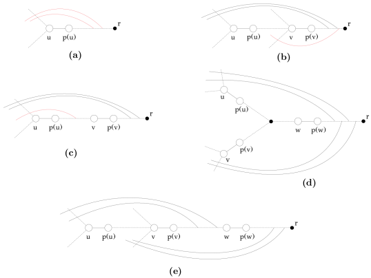
Figure 1: The types of $3$-cuts with respect to a DFS-tree. (a) One tree-edge $(u,p(u))$ and two back-edges (section 3.1). (b) Two tree-edges $(u,p(u))$ and $(v,p(v))$, where $u$ is a descendant of $v$, and one-back edge in $B(v)\setminus B(u)$ (section 3.2.1). (c) Two tree-edges $(u,p(u))$ and $(v,p(v))$, where $u$ is a descendant of $v$, and one-back edge in $B(u)\setminus B(v)$ (section 3.2.2). (d) Three tree-edges $(u,p(u))$, $(v,p(v))$ and $(w,p(w))$, where $w$ is an ancestor of $u$ and $v$, but $u$ and $v$ are not related as ancestor and descendant (section 3.3.1). (d) Three tree-edges $(u,p(u))$, $(v,p(v))$ and $(w,p(w))$, where $u$ is a descendant of $v$ and $v$ is a descendant of $w$ (section 3.3.2).

3.1 One tree-edge and two back-edges

Lemma 3.1.

Let $\{(u,p(u)),e,e^{\prime}\}$ be a $3$-cut such that $e$ and $e^{\prime}$ are back-edges. Then $B(u)=\{e,e^{\prime}\}$. Conversely, if for a vertex $u\neq r$ we have $B(u)=\{e,e^{\prime}\}$ where $e$ and $e^{\prime}$ are back-edges, then $\{(u,p(u)),e,e^{\prime}\}$ is a $3$-cut.

Proof.

After removing the tree-edge $(u,p(u))$, the edges that connect $T(u)$ with the rest of the graph are precisely those contained in $B(u)$. Let $e$ and $e^{\prime}$ be two back-edges in $B(u)$. Then it is obvious that $\{(u,p(u)),e,e^{\prime}\}$ is a $3$-cut if and only if $B(u)$ consists precisely of these two back-edges. ∎

Thus, to find all $3$-cuts of the form $\{(u,p(u)),e,e^{\prime}\}$, where $e$ and $e^{\prime}$ are back-edges, we only have to store, for every vertex $u$, two back-edges $e,e^{\prime}\in B(u)$. Since $(\mathit{low1D}(u),\mathit{low1}(u))$ and $(\mathit{low2D}(u),\mathit{low2}(u))$ are two such back-edges, we mark the triplet $\{(u,p(u)),(\mathit{low1D}(u),\mathit{low1}(u)),\linebreak(\mathit{low2D}(u),\mathit{low2}(u))\}$, for every $u$ that has $\mathit{b\_count}(u)=2$.

3.2 Two tree-edges and one back-edge

Lemma 3.2.

Let $\{(u,p(u)),(v,p(v)),e\}$ be a $3$-cut such that $e$ is a back-edge. Then $u$ and $v$ are related as ancestor and descendant.

Proof.

Suppose that $u$ and $v$ are not related as ancestor or descendant. Since the graph is $3$-edge-connected, $\mathit{b\_count}(u)>1$, and therefore there is least one back-edge $(x,y)\in B(u)\setminus\{e\}$. Since $v$ is not a descendant of $u$, $v\notin T[x,u]$; and since $v$ is not an ancestor of $u$, $v\notin T[p(u),y]$. Thus, by removing the edges $(u,p(u))$, $(v,p(v))$, and $e$, from the graph, $u$ remains connected with $p(u)$, through the path $T[u,x],(x,y),T[p(u),y]$. This contradicts that fact that $\{(u,p(u)),(v,p(v)),e\}$ is a $3$-cut. ∎

Proposition 3.3.

Let $\{(u,p(u)),(v,p(v)),e\}$ be a $3$-cut, where $e$ is a back-edge. Then, either $(1)$ $B(v)=B(u)\sqcup\{e\}$ or $(2)$ $B(u)=B(v)\sqcup\{e\}$. Conversely, if there exists a back-edge $e$ such that $(1)$ or $(2)$ is true, then $\{(u,p(u)),(v,p(v)),e\}$ is a $3$-cut.

Proof.

($\Rightarrow$) By Lemma 3.2, we may assume, without loss of generality, that $v$ is an ancestor of $u$. Now, suppose that $(1)$ does not hold; we will prove that $(2)$ does. Since $(1)$ is not true, there must exist a back-edge $e^{\prime}$ such that $e^{\prime}\in B(v)$ and $e^{\prime}\notin B(u)\cup\{e\}$, or $e^{\prime}\notin B(v)$ and $e^{\prime}\in B(u)\cup\{e\}$. Suppose the first is true: that is, there exists a back-edge $(x,y)$ such that $(x,y)\in B(v)$ and $(x,y)\notin B(u)\cup\{e\}$. Then $y$ is an ancestor of $v$, and therefore an ancestor of $u$. But, since $(x,y)\notin B(u)$, $x$ cannot be a descendant of $u$, and thus it belongs to $T(v)\setminus T(u)$. Now, by removing the edges $(u,p(u))$, $(v,p(v))$ and $e$ from the graph, we can see that $v$ remains connected with $p(v)$ through the path $T[v,x],(x,y),T[y,p(v)]$. This contradicts the fact that $\{(u,p(u)),(v,p(v)),e\}$ is a $3$-cut. Thus we have shown that there exists a back-edge $e^{\prime}$ such that $e^{\prime}\notin B(v)$ and $e^{\prime}\in B(u)\cup\{e\}$, and also that $B(v)\subseteq B(u)\cup\{e\}$. Now, suppose that there exists a back-edge $(x,y)\neq e$ such that $(x,y)\notin B(v)$ and $(x,y)\in B(u)$. Then $x$ is a descendant of $u$, and therefore a descendant of $v$. But, since $(x,y)\notin B(v)$, $y$ is not a proper ancestor of $v$, and thus belongs to $T[p(u),v]$. Now, by removing the edges $(u,p(u))$, $(v,p(v))$ and $e$ from the graph, we can see that $u$ remains connected with $p(u)$ through the path $T[u,x],(x,y),T[y,p(u)]$. This contradicts the fact that $\{(u,p(u)),(v,p(v)),e\}$ is a $3$-cut. Thus we have shown that $e$ is the unique back-edge such that $e\notin B(v)$ and $e\in B(u)$, and also that $B(u)\subseteq B(v)\cup\{e\}$. In conjunction with $B(v)\subseteq B(u)\cup\{e\}$, this implies that $B(u)=B(v)\sqcup\{e\}$.
($\Leftarrow$) First, observe that both $(1)$ and $(2)$ imply that $u$ and $v$ are related as ancestor and descendant: Since the graph is $2$-edge-connected, we have $\mathit{b\_count}(x)>0$, for every vertex $x\neq r$; and whenever we have $B(u)\cap B(v)\neq\emptyset$, for two vertices $u$ and $v$, (and such is the case if either $(1)$ or $(2)$ is true), we can infer that $u$ and $v$ are related as ancestor and descendant. Now, due to the symmetry of the relations $(1)$ and $(2)$, we may assume, without loss of generality, that $v$ is an ancestor of $u$. Let’s assume first that $(1)$ is true, and let $e=(x,y)$. Since $(x,y)\in B(v)$, $y$ is a proper ancestor of $v$, and therefore a proper ancestor of $u$. But, since $(x,y)\notin B(u)$, $x$ cannot be a descendant of $u$, and thus it belongs to $T(v)\setminus T(u)$. Furthermore, this is the only back-edge that starts from $T(v)\setminus T(u)$ and ends in a proper ancestor of $v$, since $B(v)\setminus\{e\}=B(u)$. Thus we can see that, by removing the edges $(u,p(u))$, $(v,p(v))$ and $e$ from the graph, the graph becomes disconnected. (For the subgraph $T(v)\setminus T(u)$ becomes disconnected from $T(u)\cup(T(r)\setminus T(v))$.) Now assume that $(2)$ is true, and let $e=(x,y)$. Since $(x,y)\in B(u)$, $x$ is a descendant of $u$, and therefore a descendant of $v$. But, since $(x,y)\notin B(v)$, $y$ is not a proper ancestor of $v$, and thus it belongs to $T[p(u),v]$. Furthermore, it is the only back-edge that starts from $T(u)$ and ends in $T[p(u),v]$, since $B(u)\setminus\{e\}=B(v)$. Thus we can see that, by removing the edges $(u,p(u))$, $(v,p(v))$ and $e$ from the graph, the graph becomes disconnected. (For the subgraph $T(v)\setminus T(u)$ becomes disconnected from $T(u)\cup(T(r)\setminus T(v))$.) ∎

Here we distinguish two cases, depending on whether $B(v)=B(u)\sqcup\{e\}$ or $B(u)=B(v)\sqcup\{e\}$.

3.2.1 $v$ is an ancestor of $u$ and $B(v)=B(u)\sqcup\{e\}$.

Throughout this section let $V(u)$ denote the set of vertices $v$ that are ancestors of $u$ and such that $B(v)=B(u)\sqcup\{e\}$, for a back-edge $e$. By proposition 3.3, this means that $\{(u,p(u)),(v,p(v)),e\}$ is a $3$-cut. The following lemma shows that, for every vertex $v$, there is at most one vertex $u$ such that $v\in V(u)$.

Lemma 3.4.

Let $u,u^{\prime}$ be two distinct vertices. Then $V(u)\cap V(u^{\prime})=\emptyset$.

Proof.

Suppose that there exists a $v\in V(u)\cap V(u^{\prime})$. Then there are back-edges $e,e^{\prime}$ such that $B(v)=B(u)\sqcup\{e\}$ and $B(v)=B(u^{\prime})\sqcup\{e^{\prime}\}$, and so we have $B(u)\sqcup\{e\}=B(u^{\prime})\sqcup\{e^{\prime}\}$. Since $\mathit{b\_count}(u)>1$ and $\mathit{b\_count}(u^{\prime})>1$ (for the graph is $3$-edge-connected), we infer that $B(u)\cap B(u^{\prime})\neq\emptyset$, and thus $u$ and $u^{\prime}$ are related as ancestor and descendant. Thus we can assume, without loss of generality, that $u^{\prime}$ is an ancestor of $u$. Now let $(x,y)\in B(u)$. Then $x$ is a descendant of $u$, and therefore a descendant of $u^{\prime}$. Furthermore, since $B(v)=B(u)\sqcup\{e\}$, we have $(x,y)\in B(v)$, and so $y$ is a proper ancestor of $v$, and therefore a proper ancestor of $u^{\prime}$. This shows that $(x,y)\in B(u^{\prime})$, and thus we have $B(u)\subseteq B(u^{\prime})$. In conjunction with $B(u)\sqcup\{e\}=B(u^{\prime})\sqcup\{e^{\prime}\}$ (which implies that $|B(u)|=|B(u^{\prime})|$), we infer that $B(u)=B(u^{\prime})$ (and $e=e^{\prime}$). This contradicts the fact that the graph is $3$-edge-connected. ∎

Thus, the total number of $3$-cuts of the form $\{(u,p(u)),(v,p(v)),e\}$, where $u$ is a descendant of $v$ and $e$ is a back-edge such that $B(v)=B(u)\sqcup\{e\}$, is $O(n)$. Now we will show how to compute, for every vertex $v$, the vertex $u$ such that $v\in V(u)$ (if such a vertex $u$ exists), together with the back-edge $e$ such that $\{(u,p(u)),(v,p(v)),e\}$ is a $3$-cut, in total linear time.

Let $u,v,e$ be such that $v\in V(u)$ and $B(v)=B(u)\sqcup\{e\}$, and let $e=(x,y)$. Then $y$ is a proper ancestor of $v$, and therefore a proper ancestor of $u$, so $x$ cannot be a descendant of $v$ (since $e\notin B(u)$). Thus, $x$ is either on the tree-path $T(u,v]$, or it is a proper descendant of a vertex in $T(u,v]$, but not a descendant of $u$. In the first case we have $\tilde{M}(v)=M(u)$ (and $x=M(v)$); in the second case either $M_{low1}(v)=M(u)$ (and $x=M_{low2}(v)$) or $M_{low2}(v)=M(u)$ (and $x=M_{low1}(v)$). (For an illustration, see figure 2.) The following lemma shows how we can determine $u$ from $v$.

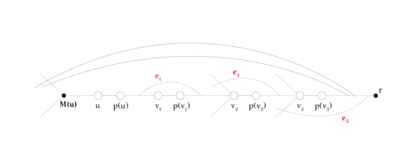
Figure 2: In this example we have $V(u)=\{v_{1},v_{2},v_{3}\}$, and every back-edge $e_{i}$ satisfies $B(v_{i})=B(u)\sqcup\{e_{i}\}$. It should be clear that every $M(v_{i})$ is an ancestor of $M(u)$, and $\tilde{M}(v_{1})=M(u)$, $M_{low1}(v_{2})=M(u)$ and $M_{low2}(v_{3})=M(u)$. It is perhaps worth noting that, for every vertex $u$, we may have many vertices $v\in V(u)$ with $\tilde{M}(v)=M(u)$ or $M_{low1}(v)=M(u)$, but only the lowest $v$ in $V(u)$ may have $M_{low2}(v)=M(u)$.

Lemma 3.5.

Let $v$ be an ancestor of $u$ such that $\tilde{M}(v)=M(u)$ or $M_{low1}(v)=M(u)$ or $M_{low2}(v)=M(u)$, and let $m$ $=$ $\tilde{M}(v)$ or $M_{low1}(v)$ or $M_{low2}(v)$, depending on whether $\tilde{M}(v)=M(u)$ or $M_{low1}(v)=M(u)$ or $M_{low2}(v)=M(u)$. Then, $v\in V(u)$ if and only if $u$ is the lowest element in $M^{-1}(m)$ which is greater than $v$ and such that $\mathit{high}(u)<v$ and $\mathit{b\_count}(v)=\mathit{b\_count}(u)+1$.

Proof.

($\Rightarrow$) $v\in V(u)$ means that there exists a back-edge $e$ such that $B(v)=B(u)\sqcup\{e\}$. Thus we get immediately $\mathit{b\_count}(v)=\mathit{b\_count}(u)+1$ as a consequence. Furthermore, since $B(u)\subset B(v)$, we also get $\mathit{high}(u)<v$ (since for every $(x,y)\in B(u)$ it must be the case that $y$ is a proper ancestor of $v$, and therefore $\mathit{high}(u)$ is a proper ancestor of $v$). Now, suppose that there exists a $u^{\prime}\in M^{-1}(m)$ which is lower than $u$ and greater than $v$. Then, since $B(u)=B(u^{\prime})$ (and, in particular, $B(u^{\prime})\subset B(u)$), there is a back-edge $(x,y)\in B(u)$ with $x\in T(u)$ and $y\in T[p(u),u^{\prime}]$. But this contradicts the fact that $\mathit{high}(u)<v$.
($\Leftarrow$) Let $(x,y)\in B(u)$. Then $x$ is a descendant of $u$, and therefore a descendant of $v$. Furthermore, $\mathit{high}(u)<v$ implies that $y$ is a proper ancestor of $v$. This shows that $(x,y)\in B(v)$, and thus we have $B(u)\subseteq B(v)$. Then, $\mathit{b\_count}(v)=\mathit{b\_count}(u)+1$ implies the existence of a back-edge $e\in B(v)\setminus B(u)$ such that $B(v)=B(u)\sqcup\{e\}$. ∎

Thus, for every vertex $v$, we have to check whether the lowest element $u$ of $M^{-1}(m)$ which is greater than $v$ satisfies $\mathit{b\_count}(v)=\mathit{b\_count}(u)+1$, for all $m\in\{\tilde{M}(v),M_{low1}(v),M_{low2}(v)\}$. To do this efficiently, we process the vertices in a bottom-up fashion, and we keep in a variable $\mathit{currentVertex}[m]$ the lowest element of $M^{-1}(m)$ currently under consideration, so that we do not have to traverse the list $M^{-1}(m)$ from the beginning each time we process a vertex. Algorithm 5 is an implementation of this procedure.

1 initialize an array $\mathit{currentVertex}$ with $n$ entries

// $m=\tilde{M}(v)$

2 foreach vertex $x$ do $\mathit{currentVertex}[x]\leftarrow x$

3 for $v\leftarrow n$ to $v=1$ do

4       $m\leftarrow\tilde{M}(v)$

5       if $m=\emptyset$ then continue

       // find the lowest $u\in M^{-1}(m)$ which is greater than $v$

6       $u\leftarrow\mathit{currentVertex}[m]$

7       while $\mathit{nextM}(u)\neq\emptyset$ and $\mathit{nextM}(u)>v$ do $u\leftarrow\mathit{nextM}(u)$

8       $\mathit{currentVertex}[m]\leftarrow u$

       // check the condition in lemma 3.5

9       if $\mathit{high}(u)<v$ and $\mathit{b\_count}(v)=\mathit{b\_count}(u)+1$ then

10             mark the triplet $\{(u,p(u)),(v,p(v)),(M(v),l(M(v)))\}$

11       end if

12      

13 end for

// $m=M_{low1}(v)$

14 foreach vertex $x$ do $\mathit{currentVertex}[x]\leftarrow x$

15 for $v\leftarrow n$ to $v=1$ do

16       $m\leftarrow M_{low1}(v)$

17       if $m=\emptyset$ then continue

       // find the lowest $u\in M^{-1}(m)$ which is greater than $v$

18       $u\leftarrow\mathit{currentVertex}[m]$

19       while $\mathit{nextM}(u)\neq\emptyset$ and $\mathit{nextM}(u)>v$ do $u\leftarrow\mathit{nextM}(u)$

20       $\mathit{currentVertex}[m]\leftarrow u$

       // check the condition in lemma 3.5

21       if $\mathit{high}(u)<v$ and $\mathit{b\_count}(v)=\mathit{b\_count}(u)+1$ then

22             mark the triplet $\{(u,p(u)),(v,p(v)),(M_{low2}(v),l(M_{low2}(v)))\}$

23       end if

24      

25 end for

// $m=M_{low2}(v)$

26 foreach vertex $x$ do $\mathit{currentVertex}[x]\leftarrow x$

27 for $v\leftarrow n$ to $v=1$ do

28       $m\leftarrow M_{low2}(v)$

29       if $m=\emptyset$ then continue

       // find the lowest $u\in M^{-1}(m)$ which is greater than $v$

30       $u\leftarrow\mathit{currentVertex}[m]$

31       while $\mathit{nextM}(u)\neq\emptyset$ and $\mathit{nextM}(u)>v$ do $u\leftarrow\mathit{nextM}(u)$

32       $\mathit{currentVertex}[m]\leftarrow u$

33       $\mathit{currentVertex}[m]\leftarrow\mathit{prev}$

       // check the condition in lemma 3.5

34       if $\mathit{high}(u)<v$ and $\mathit{b\_count}(v)=\mathit{b\_count}(u)+1$ then

35             mark the triplet $\{(u,p(u)),(v,p(v)),(M_{low1}(v),l(M_{low1}(v)))\}$

36       end if

37      

38 end for

Algorithm 5 Find all $3$-cuts $\{(u,p(u)),(v,p(v)),e)\}$, where $u$ is a descendant of $v$ and $B(v)=B(u)\sqcup\{e\}$, for a back-edge $e$.

3.2.2 $v$ is an ancestor of $u$ and $B(u)=B(v)\sqcup\{e\}$.

Throughout this section let $U(v)$ denote the set of vertices $u$ that are descendants of $v$ and such that $B(u)=B(v)\sqcup\{e\}$, for a back-edge $e$. By proposition 3.3, this means that $\{(u,p(u)),(v,p(v)),e\}$ is a $3$-cut. The following lemma shows that, for every vertex $u$, there is at most one vertex $v$ such that $u\in U(v)$.

Lemma 3.6.

Let $v,v^{\prime}$ be two distinct vertices. Then $U(v)\cap U(v^{\prime})=\emptyset$.

Proof.

Suppose that there exists a $u\in U(v)\cap U(v^{\prime})$. Then $v$ and $v^{\prime}$ are related as ancestor and descendant, since they have a common descendant. Thus we may assume, without loss of generality, that $v^{\prime}$ is an ancestor of $v$. Let $(x,y)$ be a back-edge in $B(v^{\prime})$. Then, $y$ is a proper ancestor of $v^{\prime}$, and therefore a proper ancestor of $v$. Furthermore, $u\in U(v^{\prime})$ implies that $B(v^{\prime})\subseteq B(u)$, and therefore $(x,y)\in B(u)$. Thus, $x$ is a descendant of $u$, and therefore a descendant of $v$. This shows that $(x,y)\in B(v)$, and thus we have $B(v^{\prime})\subseteq B(v)$. Now, $u\in U(v)\cap U(v^{\prime})$ means that there exist two back-edges $e,e^{\prime}$ such that $B(u)=B(v)\sqcup\{e\}$ and $B(u)=B(v)\sqcup\{e\}$, and thus we have $B(v)\sqcup\{e\}=B(v^{\prime})\sqcup\{e^{\prime}\}$. Therefore, $|B(v)|=|B(v^{\prime})|$. In conjunction with $B(v^{\prime})\subseteq B(v)$, this implies that $B(v)=B(v^{\prime})$ (and $e=e^{\prime}$), contradicting the fact that the graph is $3$-edge-connected. ∎

Thus, the total number of $3$-cuts of the form $\{(u,p(u)),(v,p(v)),e\}$, where $u$ is a descendant of $v$ and $e$ is a back-edge such that $B(u)=B(v)\sqcup\{e\}$, is $O(n)$. We will now show how to compute, for every vertex $u$, the vertex $v$ such that $u\in U(v)$ (if such a vertex $v$ exists), together with the back-edge $e$ such that $\{(u,p(u)),(v,p(v)),e\}$ is a $3$-cut, in total linear time.

Let $u,v,e$ be such that $u\in U(v)$ and $B(u)=B(v)\sqcup\{e\}$, and let $e=(x,y)$. Then, $x$ is a descendant of $u$, and therefore a descendant of $v$. But since $e\notin B(v)$, $y$ is not an ancestor of $v$, and therefore $y\in T[p(u),v]$. Thus, $y=\mathit{high}(u)$ (and $x=\mathit{highD}(u)$), since every other back-edge $(x^{\prime},y^{\prime})\in B(u)$ is also in $B(v)$ and thus has $y^{\prime}<v\leq y$. This shows how we can determine the back-edge $e$ from a pair of vertices $u,v$ that satisfy $u\in U(v)$. Furthermore, $B(u)=B(v)\sqcup\{e\}$ implies that $M(u)$ is an ancestor of $M(v)$. Thus, either $M(u)=M(v)$, or $M(u)$ is a proper ancestor of $M(v)$. In the second case, we have that either $\tilde{M}(u)=M(v)$ or $M_{low1}(u)=M(v)$ (since the $\mathit{low}$ point of $u$ is given by a back-edge in $B(v)$). (For an illustration, see figure 3.) Now the following lemma shows how we can determine $v$ from $u$.

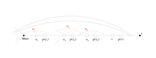
Figure 3: In this example we have $U(v)=\{u_{1},u_{2},u_{3}\}$, and every back-edge $e_{i}$ satisfies $B(u_{i})=B(v)\sqcup\{e_{i}\}$. It should be clear that every $M(u_{i})$ is an ancestor of $M(v)$, and $M(u_{1})=M(v)$, $M_{low1}(u_{2})=M(v)$ and $\tilde{M}(u_{3})=M(v)$. It is perhaps worth noting that, for every vertex $v$, only one $u\in U(v)$ may have $M(u)=M(v)$ (that is, the one satisfying $\mathit{nextM}(u)=v$), but we may have many vertices $u\in V(v)$ with $\tilde{M}(u)=M(v)$ or $M_{low1}(u)=M(v)$.

Lemma 3.7.

Let $u$ be a descendant of $v$ such that $M(u)=M(v)$ or $\tilde{M}(u)=M(v)$ or $M_{low1}(u)=M(v)$, and let $m$ $=$ $M(u)$ or $\tilde{M}(u)$ or $M_{low1}(u)$, depending on whether $M(u)=M(v)$ or $\tilde{M}(u)=M(v)$ or $M_{low1}(u)=M(v)$. Then $u\in U(v)$ if and only if $v$ is the greatest element in $M^{-1}(m)$ which is lower than $u$ and such that $\mathit{b\_count}(u)=\mathit{b\_count}(v)+1$.

Proof.

($\Rightarrow$) $u\in U(v)$ means that there exists a back-edge $e$ such that $B(u)=B(v)\sqcup\{e\}$. Thus we get immediately that $\mathit{b\_count}(u)=\mathit{b\_count}(v)+1$. Now suppose, for the sake of contradiction, that there exists a $v^{\prime}\in M^{-1}(m)$ which is greater than $v$ and lower than $u$. Let $(x,y)\in B(v^{\prime})$. Then $y$ is a proper ancestor of $v^{\prime}$, and therefore a proper ancestor of $u$. Furthermore, $x$ is a descendant of $M(v^{\prime})$ ($=M(v)$), and so every one of the relations $M(u)=M(v)$, $\tilde{M}(u)=M(v)$ or $M_{low1}(u)=M(v)$ implies that $x$ is a descendant of $u$. This shows that $(x,y)\in B(u)$, and thus we have $B(v^{\prime})\subseteq B(u)$. Now, since $M(v)=M(v^{\prime})$ and $v^{\prime}$ is a proper ancestor of $v$, we have $B(v)\subset B(v^{\prime})$. Since $\mathit{b\_count}(u)=\mathit{b\_count}(v)+1$, $B(v)\subset B(v^{\prime})\subseteq B(u)$ implies that $B(u)=B(v^{\prime})$, contradicting the fact that the graph is $3$-edge-connected.
($\Leftarrow$) Let $(x,y)\in B(v)$. Then $y$ is a proper ancestor of $v$, and therefore a proper ancestor of $u$. Furthermore, $x$ is a descendant of $M(v)$, and every one of the relations $M(u)=M(v)$, $\tilde{M}(u)=M(v)$ or $M_{low1}(u)=M(v)$ implies that $x$ is a descendant of $M(u)$. This shows that $(x,y)\in B(u)$. Thus we have $B(v)\subseteq B(u)$, and so $\mathit{b\_count}(u)=\mathit{b\_count}(v)+1$ implies that there exists a back-edge $e$ such $B(u)=B(v)\sqcup\{e\}$. ∎

Thus, for every vertex $u$, we have to check whether the greatest element $v$ in $M^{-1}(m)$ which is lower than $u$ satisfies $\mathit{b\_count}(u)=\mathit{b\_count}(v)+1$, for all $m\in\{M(u),\tilde{M}(u),M_{low1}(u)\}$. To do this efficiently, we process the vertices in a bottom-up fashion, and we keep in a variable $\mathit{currentVertex}[m]$ the lowest element of $M^{-1}(m)$ currently under consideration, so that we do not have to traverse the list $M^{-1}(m)$ from the beginning each time we process a vertex. Algorithm 6 is an implementation of this procedure.

1 initialize an array $\mathit{currentVertex}$ with $n$ entries

// $m=M(v)$; just check whether the condition of Lemma 3.7 is satisfied for $\mathit{nextM}(u)$

2 if $\mathit{b\_count}(u)=\mathit{b\_count}(\mathit{nextM}(u))+1$ then

3       mark the triplet $\{(u,p(u)),(\mathit{nextM}(u),p(\mathit{nextM}(u))),(\mathit{highD}(u),\mathit{high}(u))\}$

4 end if

// $m=\tilde{M}(u)$

5 foreach vertex $x$ do $\mathit{currentVertex}[x]\leftarrow x$

6 for $u\leftarrow n$ to $u=1$ do

7       $m\leftarrow\tilde{M}(u)$

8       if $m=\emptyset$ then continue

       // find the greatest $v\in M^{-1}(m)$ which is lower than $u$

9       $v\leftarrow\mathit{currentVertex}[m]$

10       while $v\neq\emptyset$ and $v\geq u$ do $v\leftarrow\mathit{nextM}(v)$

11       $\mathit{currentVertex}[m]\leftarrow v$

       // check the condition in Lemma 3.7

12       if $\mathit{b\_count}(u)=\mathit{b\_count}(v)+1$ then

13             mark the triplet $\{(u,p(u)),(v,p(v)),(\mathit{highD}(u),\mathit{high}(u))\}$

14       end if

15      

16 end for

// $m=M_{low1}(u)$

17 foreach vertex $x$ do $\mathit{currentVertex}[x]\leftarrow x$

18 for $u\leftarrow n$ to $u=1$ do

19       $m\leftarrow M_{low1}(u)$

20       if $m=\emptyset$ then continue

       // find the greatest $v\in M^{-1}(m)$ which is lower than $u$

21       $v\leftarrow\mathit{currentVertex}[m]$

22       while $v\neq\emptyset$ and $v\geq u$ do $v\leftarrow\mathit{nextM}(v)$

23       $\mathit{currentVertex}[m]\leftarrow v$

       // check the condition in Lemma 3.7

24       if $\mathit{b\_count}(u)=\mathit{b\_count}(v)+1$ then

25             mark the triplet $\{(u,p(u)),(v,p(v)),(\mathit{highD}(u),\mathit{high}(u))\}$

26       end if

27      

28 end for

Algorithm 6 Find all $3$-cuts $\{(u,p(u)),(v,p(v)),e)\}$, where $u$ is a descendant of $v$ and $B(u)=B(v)\sqcup\{e\}$, for a back-edge $e$.

3.3 Three tree-edges

Lemma 3.8.

Let $\{(u,p(u)),(v,p(v)),(w,p(w))\}$ be a $3$-cut, and assume, without loss of generality, that $w<\mathit{min}\{v,u\}$. Then $w$ is an ancestor of both $u$ and $v$.

Proof.

Suppose that $w$ is neither an ancestor of $u$ nor an ancestor of $v$. Let $(x,y)\in B(w)$. Then $x$ is a descendant of $w$, and therefore it is not a descendant of either $u$ or $v$. In other words, $u,v\notin T[x,w]$. Furthermore, $y$ is a proper ancestor of $w$. Since neither $u$ nor $v$ is an ancestor of $w$ (since $w<\mathit{min}\{v,u\}$), we have that $u,v\notin T[w,r]$, and therefore $u,v\notin T[w,y]$. Thus, by removing the tree-edges $(u,p(u))$, $(v,p(v))$ and $(w,p(w))$, $w$ remains connected with $p(w)$ through the path $T[w,x],(x,y),T[y,p(w)]$, contradicting the fact that $\{(u,p(u)),(v,p(v)),(w,p(w))\}$ is a $3$-cut. This shows that $w$ is an ancestor of either $u$ or $v$ (or both). Suppose, for the sake of contradiction, that $w$ is not an ancestor of $u$. Then $w$ is an ancestor of $v$. This implies that $u$ is not a descendant of $v$ (for otherwise it would be a descendant of $w$). If $u$ is an ancestor of $v$, it must necessarily be an ancestor of $w$ (because $v\in T(w)$ and $u\notin T(w)$), but $w<u$ forbids this case. Thus, $u$ is not a ancestor of $v$. So far, then, we have that $u$ is not related as ancestor and descendant with either $w$ or $v$. Thus we may follow the same reasoning as above, to conclude that, by removing the tree-edges $(u,p(u))$, $(v,p(v))$ and $(w,p(w))$, $u$ remains connected with $p(u)$, again contradicting the fact that $\{(u,p(u)),(v,p(v)),(w,p(w))\}$ is a $3$-cut. This shows that $w$ is an ancestor of $u$. Using the same argument we can also prove that $w$ is an ancestor of $v$. ∎

At this point we distinguish two cases, depending on whether $u$ and $v$ are related as ancestor and descendant.

3.3.1 $u$ and $v$ are not related as ancestor and descendant

In what follows we will provide some characterizations of the $3$-cuts of the form $\{(u,p(u)),(v,p(v)),(w,p(w))\}$, where $w$ is an ancestor of $u$ and $v$, and $u,v$ are not related as ancestor and descendant. It will be useful to keep in mind the situation depicted in Figure 4.

Proposition 3.9.

Let $u$ and $v$ be two vertices which are not related as ancestor and descendant, and let $w$ be an ancestor of both $u$ and $v$. Then, $\{(u,p(u)),(v,p(v)),(w,p(w))\}$ is a $3$-cut if and only if $B(w)=B(u)\sqcup B(v)$.

Proof.

($\Rightarrow$) Let $(x,y)\in B(w)$, and let’s assume that $(x,y)\notin B(u)$. Since $y$ is a proper ancestor of $w$, and therefore a proper ancestor of $u$, from $(x,y)\notin B(u)$ we infer that $x$ is not a descendant of $u$. Suppose for the sake of contradiction that $x$ is not a descendant of $v$, either. This means that neither $u$ nor $v$ is in $T[x,w]$, and so, by removing the edges $(u,p(u))$, $(v,p(v))$ and $(w,p(w))$, $w$ remains connected with $p(w)$ through the path $T[w,x],(x,y),T[y,p(w)]$. This contradicts that fact that $\{(u,p(u)),(v,p(v)),(w,p(w))\}$ is a $3$-cut. Thus we have established that $x$ is a descendant of $v$. Since $y$ is also a proper ancestor of $v$, we have $(x,y)\in B(v)$. Thus we have shown that $B(w)\subseteq B(u)\cup B(v)$. Conversely, let $(x,y)\in B(u)\cup B(v)$, and assume, without loss of generality, that $(x,y)\in B(u)$. Then, $x$ is a descendant of $u$, and therefore a descendant of $w$. Now suppose, for the sake of contradiction, that $y$ is not a proper ancestor of $w$. Then we have $w\notin T[p(u),y)$, and since $w$ is not a descendant of $u$, we also have $w\notin T[x,u]$. Furthermore, since $u$ and $v$ are not related as ancestor and descendant, $v$ is not contained neither in $T[p(u),y)$ nor in $T[x,u]$. Thus, by removing the edges $(u,p(u))$, $(v,p(v))$ and $(w,p(w))$, $u$ remains connected with $p(u)$ through the path $T[u,x],(x,y),T[y,p(u)]$. This contradicts that fact that $\{(u,p(u)),(v,p(v)),(w,p(w))\}$ is a $3$-cut. Thus we have shown that $y$ is a proper ancestor of $w$, and so we have that $(x,y)\in B(w)$. Thus we have established that $B(u)\cup B(v)\subseteq B(w)$, and so we have $B(w)=B(u)\cup B(v)$. Since $u$ and $v$ are not related as ancestor and descendant, we have $B(u)\cap B(v)=\emptyset$. We conclude that $B(w)=B(u)\sqcup B(v)$.
($\Leftarrow$) Consider the sets of vertices $T(u)$, $T(v)$, $A=T(w)\setminus(T(u)\cup T(v))$ and $B=T(r)\setminus T(w)$. Since $u$ and $v$ are not related as ancestor and descendant, and $w$ is an ancestor of both $u$ and $v$, these sets are mutually disjoint. Now, since $B(u)\subset B(w)$, all back-edges that start from $T(u)$ end either in $T(u)$ or in $B$. Similarly, since $B(v)\subset B(w)$, all back-edges that start from $T(v)$ end either in $T(v)$ or in $B$. Furthermore, a back-edge that starts from $A$ cannot reach $B$ and must necessarily end in $A$, since it starts from a descendant of $w$, but not from a descendant of either $u$ or $v$ (while we have $B(w)=B(u)\sqcup B(v)$). Thus, by removing from the graph the tree-edges $(u,p(u))$, $(v,p(v))$ and $(w,p(w))$, the graph becomes separated into two parts: $T(u)\cup T(v)\cup B$ and $A$. ∎

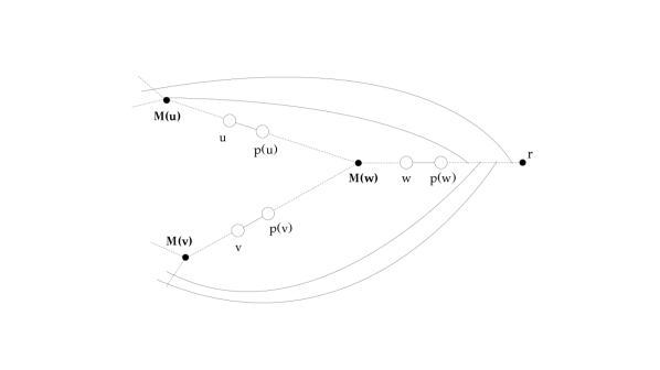
Figure 4: In this example we have $B(w)=B(u)\sqcup B(v)$. Observe that $M_{low1}(w)=M(u)$ and $M_{low2}(w)=M(v)$. Furthermore, $\mathit{high}(u)<w$ and $\mathit{high}(v)<w$. Also, if there is another vertex $u^{\prime}$ with $M(u^{\prime})=M(u)$, it must either be a descendant of $u$ or an ancestor of $w$. Thus, $u$ is the lowest vertex in $M^{-1}(M_{low1}(w))$ which is greater than $w$. Similarly, $v$ is the lowest vertex in $M^{-1}(M_{low2}(w))$ which is greater than $w$. By Lemmata 3.10 and 3.11, these properties (together with $\mathit{b\_count}(w)=\mathit{b\_count}(u)+\mathit{b\_count}(v)$) are sufficient to establish $B(w)=B(u)\sqcup B(v)$. Notice also that, if we remove the tree-edges $(u,p(u))$, $(v,p(v))$ and $(w,p(w))$, the graph becomes disconnected into two components: $T(u)\cup T(v)\cup(T(r)\setminus T(w))$ and $T(w)\setminus(T(u)\cup T(v))$. (See also the “$\Leftarrow$” part of the proof of proposition 3.9.)

Lemma 3.10.

Let $u$ and $v$ be two vertices which are not related as ancestor and descendant, and let $w$ be an ancestor of both $u$ and $v$. Then $B(w)=B(u)\sqcup B(v)$ if and only if: $M_{low1}(w)=M(u)$ and $M_{low2}(w)=M(v)$ (or $M_{low1}(w)=M(v)$ and $M_{low2}(w)=M(u)$), and $\mathit{high}(u)<w$, $\mathit{high}(v)<w$, and $\mathit{b\_count}(w)=\mathit{b\_count}(u)+\mathit{b\_count}(v)$.

Proof.

($\Rightarrow$) $\mathit{b\_count}(w)=\mathit{b\_count}(u)+\mathit{b\_count}(v)$ is an immediate consequence of $B(w)=B(u)\sqcup B(v)$. Furthermore, since every $(x,y)\in B(u)$ is also in $B(w)$, it has $y<w$, and so $\mathit{high}(u)<w$. With the same reasoning, we also get $\mathit{high}(v)<w$. Now, since $B(w)=B(u)\sqcup B(v)$, we have that $M(w)$ is an ancestor of both $M(u)$ and $M(v)$. Since $u$ and $v$ are not related as ancestor and descendant, $M(u)$ and $M(v)$ are not related as ancestor or descendant, either. This implies that they are both proper descendants of $M(w)$. Now, suppose, for the sake of contradiction, that $M(u)$ and $M(v)$ are descendants of the same child $c$ of $M(w)$. Then there must exist a back-edge $(x,y)\in B(w)$ such that $x=M(w)$ or $x$ is a descendant of a child of $M(w)$ different from $c$. (Otherwise, $M(w)$ would be a descendant of $c$, which is absurd.) But this contradicts the fact that $B(w)=B(u)\sqcup B(v)$, since $(x,y)$ does not belong neither in $B(u)$ nor in $B(v)$. Thus, $M(u)$ and $M(v)$ are descendants of different children of $M(w)$. Furthermore, since every back-edge $(x,y)\in B(w)$ has $x$ in $T(u)$ or $T(v)$, there are no other children of $M(w)$ from whose subtrees begin back-edges that end in a proper ancestor of $w$. Thus, one of $M(u)$ and $M(v)$ is a descendant of the $\mathit{low1}$ child of $M(w)$, and the other is a descendant of the $\mathit{low2}$ child of $M(w)$. We may assume, without loss of generality, that $M(u)$ is a descendant of the $\mathit{low1}$ child of $M(w)$, and $M(v)$ is a descendant of the $\mathit{low2}$ child of $M(w)$. Since $B(u)\subset B(w)$, we have that $M(u)$ is a descendant of $M_{low1}(w)$. Furthermore, since $B(w)=B(u)\sqcup B(v)$ and $M(v)$ is not a descendant of the $\mathit{low1}$ child of $M(w)$, there are no back-edges $(x,y)$ with $x$ a descendant of the $\mathit{low1}$ child of $M(w)$ and $y$ a proper ancestor of $w$ apart from those contained in $B(u)$. Thus, $M(u)$ is an ancestor of $M_{low1}(w)$, and $M_{low1}(w)=M(u)$ is established. With the same reasoning, we also get $M_{low2}(w)=M(v)$.
($\Leftarrow$) Let $(x,y)\in B(u)$. Then $x$ is a descendant of $u$, and therefore a descendant of $w$. Furthermore, since $\mathit{high}(u)<w$, we have $y<w$, and therefore $y$ is a proper ancestor of $w$. This shows that $(x,y)\in B(w)$, and thus $B(u)\subseteq B(w)$. With the same reasoning, we also get $B(v)\subseteq B(w)$. Thus we have $B(u)\cup B(v)\subseteq B(w)$. Since $u$ and $v$ are not related as ancestor and descendant, we have $B(u)\cap B(v)=\emptyset$. From $B(u)\cup B(v)\subseteq B(w)$, $B(u)\cap B(v)=\emptyset$, and $\mathit{b\_count}(w)=\mathit{b\_count}(u)+\mathit{b\_count}(v)$, we conclude that $B(w)=B(u)\sqcup B(v)$. ∎

The following lemma shows, that, for every vertex $w$, there is at most one pair $u,v$ of descendants of $w$ which are not related as ancestor and descendant and are such that $\{(u,p(u)),(v,p(v)),(w,p(w))\}$ is a $3$-cut. Thus, the number of $3$-cuts of this type is $O(n)$. Furthermore, it allows us to compute $u$ and $v$ (if such a pair of $u$ and $v$ exists).

Lemma 3.11.

Let $\{(u,p(u)),(v,p(v)),(w,p(w))\}$ be a $3$-cut such that $u$ and $v$ are not related as ancestor and descendant and let $w$ is an ancestor of both $u$ and $v$. Assume w.l.o.g. that $M_{low1}(w)=M(u)$ and $M_{low2}(w)=M(v)$, and let $m_{1}=M_{low1}(w)$ and $m_{2}=M_{low2}(w)$. Then $u$ is the lowest vertex in $M^{-1}(m_{1})$ which is greater than $w$, and $v$ is the lowest vertex in $M^{-1}(m_{2})$ which is greater that $w$.

Proof.

By Proposition 3.9, we have that $B(w)=B(u)\sqcup B(v)$. Now, suppose that there exists a $u^{\prime}\in M^{-1}(m_{1})$ which is lower than $u$ and greater than $w$. Then, $M(u^{\prime})=M(u)$ implies that $B(u^{\prime})\subset B(u)$, and so there is a back-edge $(x,y)\in B(u)\setminus B(u^{\prime})$. This means that $y$ is not a proper ancestor of $u^{\prime}$, and therefore not a proper ancestor of $w$, either. But this implies that $(x,y)\notin B(w)$, contradicting the fact that $B(u)\subset B(w)$. A similar argument shows that there does not exist a $v^{\prime}\in M^{-1}(m_{2})$ which is lower than $v$ and greater than $w$. ∎

Thus we only have to find, for every vertex $w$, the lowest element $u$ of $M^{-1}(M_{low1}(w))$ which is greater than $w$, and the lowest element $v$ of $M^{-1}(M_{low2}(w))$ which is greater than $w$, and check the condition in Lemma 3.10 - i.e., whether $\mathit{high}(u)<w$, $\mathit{high}(v)<w$, and $\mathit{b\_count}(w)=\mathit{b\_count}(u)+\mathit{b\_count}(v)$. To do this efficiently, we process the vertices in a bottom-up fashion, and we keep in a variable $\mathit{currentVertex}[x]$ the lowest element of $M^{-1}(x)$ currently under consideration. Thus, we do not need to traverse the list $M^{-1}(x)$ from the beginning each time we process a vertex. Algorithm 7 is an implementation of this procedure.

1 initialize an array $\mathit{currentVertex}$ with $n$ entries

2 foreach vertex $x$ do $\mathit{currentVertex}[x]\leftarrow x$

3 for $w\leftarrow n$ to $w=1$ do

4       $m_{1}\leftarrow M_{low1}(w)$, $m_{2}\leftarrow M_{low2}(w)$

5      

6      if $m_{1}=\emptyset$ or $m_{2}=\emptyset$ then continue

7      

      // find the lowest $u$ in $M^{-1}(m_{1})$ which is greater than $w$

8       $u\leftarrow\mathit{currentVertex}[m_{1}]$

9       while $\mathit{nextM}(u)\neq\emptyset$ and $\mathit{nextM}(u)>w$ do $u\leftarrow\mathit{nextM}(u)$

10       $\mathit{currentVertex}[m_{1}]\leftarrow u$

11      

      // find the lowest $v$ in $M^{-1}(m_{2})$ which is greater than $w$

12       $v\leftarrow\mathit{currentVertex}[m_{2}]$

13       while $\mathit{nextM}(v)\neq\emptyset$ and $\mathit{nextM}(v)>w$ do $v\leftarrow\mathit{nextM}(v)$

14       $\mathit{currentVertex}[m_{2}]\leftarrow v$

15      

      // check the condition in Lemma 3.10

16       if $\mathit{b\_count}(w)=\mathit{b\_count}(u)+\mathit{b\_count}(v)$ and $\mathit{high}(u)<w$ and $\mathit{high}(v)<w$ then

17             mark the triplet $\{(u,p(u)),(v,p(v)),(w,p(w))\}$

18            

19       end if

20      

21 end for

Algorithm 7 Find all $3$-cuts $\{(u,p(u)),(v,p(v)),(w,p(w))\}$, where $w$ is an ancestor of $u$ and $v$, and $u,v$ are not related as ancestor and descendant

3.3.2 $u$ and $v$ are related as ancestor and descendant

Throughout this section it will be useful to keep in mind the situation depicted in Figure 5.

Proposition 3.12.

Let $u,v,w$ be three vertices such that $u$ is a descendant of $v$ and $v$ is a descendant of $w$. Then $\{(u,p(u)),(v,p(v)),(w,p(w))\}$ is a $3$-cut if and only if $B(v)=B(u)\sqcup B(w)$.

Proof.

($\Rightarrow$) Let $(x,y)\in B(v)$, and assume that $(x,y)\notin B(u)$. $(x,y)\in B(v)$ implies that $y$ is a proper ancestor of $v$, and therefore a proper ancestor of $u$. Thus, $(x,y)\notin B(u)$ implies that $x$ is not a descendant of $u$. Furthermore, $(x,y)\in B(v)$ implies that $x$ is a descendant of $v$, and therefore a descendant of $w$. Now suppose, for the sake of contradiction, that $y$ is not a proper ancestor of $w$. Then, $w\notin T[p(v),y)$. Now we see that, by removing the edges $(u,p(u))$, $(v,p(v))$ and $(w,p(w))$ from the graph, $v$ remains connected with $p(v)$ through the path $T[v,x],(x,y),T[y,p(v)]$ (since $u,w\notin T[v,x]\cup T[p(v),y]$). This contradicts the fact that $\{(u,p(u)),(v,p(v)),(w,p(w))\}$ is a $3$-cut. Therefore, $y$ is a proper ancestor of $w$, and thus $(x,y)\in B(w)$. Thus far we have established that $B(v)\subseteq B(u)\cup B(w)$. Now let $(x,y)\in B(u)$. Then $x$ is a descendant of $u$, and therefore a descendant of $v$. Suppose, for the sake of contradiction, that $y$ is not a proper ancestor of $v$. Then, $v\notin T[p(u),y)$. Now we see that, by removing the edges $(u,p(u))$, $(v,p(v))$ and $(w,p(w))$ from the graph, $u$ remains connected with $p(u)$ through the path $T[u,x],(x,y),T[y,p(u)]$. This contradicts the fact that $\{(u,p(u)),(v,p(v)),(w,p(w))\}$ is a $3$-cut. Therefore, $y$ is a proper ancestor of $v$, and thus $(x,y)\in B(v)$. This shows that $B(u)\subseteq B(v)$. Now let $(x,y)\in B(w)$. Then $y$ is a proper ancestor of $w$, and therefore a proper ancestor of $v$. Suppose, for the sake of contradiction, that $x$ is not a descendant of $v$. Then $x$ is not a descendant of $u$, either, and so $u,v\notin T[x,w]$. Thus we see that, by removing the edges $(u,p(u))$, $(v,p(v))$ and $(w,p(w))$ from the graph, $w$ remains connected with $p(w)$ through the path $T[w,x],(x,y),T[y,p(w)]$. This contradicts the fact that $\{(u,p(u)),(v,p(v)),(w,p(w))\}$ is a $3$-cut. Therefore, $x$ is a descendant of $v$, and thus $(x,y)\in B(v)$. This shows that $B(w)\subseteq B(v)$. Thus we have established that $B(u)\cup B(w)\subseteq B(v)$, and so we have $B(v)=B(u)\cup B(w)$.

Now suppose, for the sake of contradiction, that there is a back-edge $(x,y)\in B(u)\cap B(w)$. Since $B(u)\neq B(w)$ (for otherwise $u=w$), there must exist a back-edge $(x^{\prime},y^{\prime})$ in $B(u)\setminus B(w)$ or in $B(w)\setminus B(u)$. Take the first case, first. Then, since $B(u)\subseteq B(v)$, $y^{\prime}$ is a proper ancestor of $v$. But since $(x^{\prime},y^{\prime})\notin B(w)$, $y^{\prime}$ cannot be a proper ancestor of $w$. Let $P$ be a path connecting $x^{\prime}$ with $x$ in $T(u)$. Then, by removing the tree-edges $(u,p(u))$, $(v,p(v))$ and $(w,p(w))$, $w$ remains connected with $p(w)$ through the path $T[w,y^{\prime}],(x^{\prime},y^{\prime}),P,(x,y),T[y,p(w)]$, which contradicts the assumption that $\{(u,p(u)),(v,p(v)),(w,p(w))\}$ is a $3$-cut. Now take the case $\exists(x^{\prime},y^{\prime})\in B(w)\setminus B(u)$. Then, since $B(w)\subseteq B(v)$, $x^{\prime}$ is a descendant of $v$. But since $(x^{\prime},y^{\prime})\notin B(u)$, $x^{\prime}$ cannot be a descendant of $u$. Let $P$ be a path connecting $y$ with $y^{\prime}$ in $T(r)\setminus T(w)$, and $Q$ be a path connecting $x^{\prime}$ with $p(u)$ in $T(v)\setminus T(u)$. Then, by removing the tree-edges $(u,p(u))$, $(v,p(v))$ and $(w,p(w))$, $u$ remains connected with $p(u)$ through the path $T[u,x],(x,y),P,(y^{\prime},x^{\prime}),Q$, which contradicts the assumption that $\{(u,p(u)),(v,p(v)),(w,p(w))\}$ is a $3$-cut. This shows that $B(u)\cap B(w)=\emptyset$. We conclude that $B(v)=B(u)\sqcup B(w)$.
($\Leftarrow$) Consider the sets of vertices $A=T(u)$, $B=T(v)\setminus T(u)$, $C=T(w)\setminus T(v)$ and $D=T(r)\setminus T(w)$. Since $u$ is a descendant of $v$ and $v$ is a descendant of $w$, these sets are mutually disjoint. Now, since $B(u)\subset B(v)$ and $B(u)\cap B(w)=\emptyset$, every back-edge that starts from $A$ ends either in $A$ or in $T(v,w]$, and thus in $C$. Furthermore, every back-edge that starts from $B$ and does not end in $B$, is a back-edge that starts from $T(v)$, but not from $T(u)$, and ends in a proper ancestor of $v$; thus, since $B(v)=B(u)\sqcup B(w)$, it ends in $T(w,r]$, and thus in $D$. Finally, every back-edge that starts from $C$ must end in $C$, since $B(w)\subset B(v)$. Thus we see, that, by removing from the graph the tree-edges $(u,p(u))$, $(v,p(v))$ and $(w,p(w))$, the graph becomes separated into two parts: $A\cup C$ and $B\cup D$. ∎

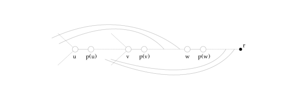
Figure 5: In this example we have $B(v)=B(u)\sqcup B(w)$. By removing the tree-edges $(u,p(u))$, $(v,p(v))$ and $(w,p(w))$, the graph becomes disconnected into two components: $T(u)\cup(T(w)\setminus T(v))$ and $(T(v)\setminus T(u))\cup(T(r)\setminus T(w))$. (See also the “$\Leftarrow$” part of the proof of proposition 3.12.)

Corollary 3.13.

If $(u,p(u))$, $(v,p(v))$ are two tree-edges, there is at most one $w$ such that $\{(u,p(u)),(v,p(v)),(w,p(w))\}$ is a $3$-cut.

Proof.

This is a consequence of propositions 3.9 and 3.12. ∎

Here we distinguish two cases, depending on whether $M(v)=M(w)$ or $M(v)\neq M(w)$.

$M(v)\neq M(w)$

Lemma 3.14.

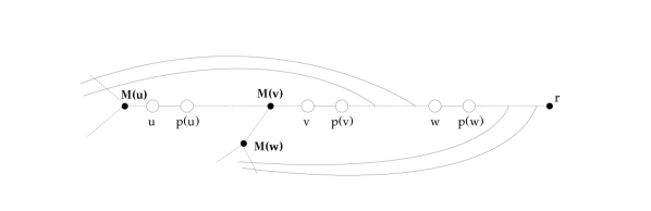
Figure 6: In this example we have $B(v)=B(u)\sqcup B(w)$. Observe that $M_{low1}(v)=M(w)$ and $M_{low2}(v)=M(u)$. $u$ is the last vertex in $M^{-1}(M(u))$, and $w$ is the greatest vertex in $M^{-1}(M(w))$ which is lower than $v$.

Let $u$ be a descendant of $v$ and $v$ a descendant of $w$, and $M(v)\neq M(w)$. Then, $\{(u,p(u)),(v,p(v)),(w,p(w))\}$ is a $3$-cut if and only if: $M(w)=M_{low1}(v)$ and $w$ is the greatest vertex with $M(w)=M_{low1}(v)$ which is lower than $v$, $M(u)=M_{low2}(v)$ and $u$ is the lowest vertex with $M(u)=M_{low2}(v)$, $\mathit{high}(u)<v$ and $\mathit{b\_count}(v)=\mathit{b\_count}(u)+\mathit{b\_count}(w)$. (See Figure 6.)

Proof.

($\Rightarrow$) By proposition 3.12, we have $B(v)=B(u)\sqcup B(w)$. This immediately establishes both $\mathit{high}(u)<v$ and $\mathit{b\_count}(v)=\mathit{b\_count}(u)+\mathit{b\_count}(w)$. Now, since $B(v)=B(u)\sqcup B(w)$, both $M(u)$ and $M(w)$ are descendants of $M(v)$. We will show that $M(u)$ and $M(w)$ are not related as ancestor and descendant. First, suppose that $M(u)$ is an ancestor of $M(w)$. Now let $(x,y)\in B(w)$. Then $x$ is a descendant of $M(w)$, and therefore a descendant of $M(u)$. Furthermore, $y$ is a proper ancestor of $w$, and therefore a proper ancestor of $u$. This shows that $(x,y)\in B(u)$, contradicting the fact that $B(u)\cap B(w)=\emptyset$. Now suppose that $M(w)$ is an ancestor of $M(u)$. Let $(x,y)\in B(v)$. Since $B(v)=B(u)\sqcup B(w)$, $x$ is a descendant of either $M(u)$ or $M(w)$. In either case, $x$ is a descendant of $w$. Due to the generality of $(x,y)$, this shows that $M(v)$ is a descendant of $M(w)$. Since $M(w)$ is also a descendant of $M(v)$, we get $M(w)=M(v)$, contradicting $M(w)\neq M(v)$. Thus we have established that $M(u)$ and $M(w)$ are not related as ancestor and descendant. Since $M(u)$ and $M(v)$ are descendants of $M(v)$, they must be proper descendants of $M(v)$. Now we will show that $M(u)$ and $M(w)$ are descendants of different children of $M(v)$. Suppose, for the sake of contradiction, that $M(u)$ and $M(w)$ are descendants of the same child $c$ of $M(v)$. Then, there must exist a back-edge $(x,y)\in B(v)$ such that $x=M(v)$ or $x$ is a descendant of a child of $M(v)$ different from $c$. (Otherwise, we would have that $M(v)$ is a descendant of $c$, which is absurd.) But this means that $(x,y)$ is neither in $B(u)$ nor in $B(w)$, contradicting the fact that $B(v)=B(u)\sqcup B(w)$. Thus, one of $M(u)$ and $M(w)$ is a descendant of the $\mathit{low1}$ child of $M(v)$, and the other is a descendant of the $\mathit{low2}$ child of $M(v)$. Observe that there does not exist a back-edge $(x,y)\in B(u)$ such that $y=\mathit{low}(v)$, for this would imply that $(x,y)\in B(w)$ (since $u$ is a descendant of $w$), and $B(u)$ does not meet $B(w)$. Thus, since $B(v)=B(u)\sqcup B(w)$, $v$ gets its $\mathit{low}$ point from $B(w)$. This shows that $M(w)$ is a descendant of the $\mathit{low1}$ child of $M(v)$ and $M(u)$ is a descendant of the $\mathit{low2}$ child of $M(v)$. Since $B(w)\subset B(v)$, we have that $M(w)$ is a descendant of $M_{low1}(v)$. Furthermore, since $B(v)=B(u)\sqcup B(w)$ and $M(u)$ is not a descendant of the $\mathit{low1}$ child of $M(v)$, there are no back-edges $(x,y)$ with $x$ a descendant of the $\mathit{low1}$ child of $M(v)$ and $y$ a proper ancestor of $v$ apart from those contained in $B(w)$. Thus, $M(w)$ is an ancestor of $M_{low1}(v)$, and $M_{low1}(v)=M(w)$ is established. With the same reasoning, we also get $M_{low2}(v)=M(u)$.

Now suppose, for the sake of contradiction, that there exists a vertex $w^{\prime}$ with $M(w^{\prime})=M(w)$ and $v>w^{\prime}>w$. This implies that $B(w)\subset B(w^{\prime})$, and thus there is a back-edge $(x,y)\in B(w^{\prime})\setminus B(w)$. Then $x$ is a descendant of $M(w^{\prime})$, and therefore a descendant of $M_{low1}(v)$. Furthermore, $y$ is a proper ancestor of $w^{\prime}$, and therefore a proper ancestor of $v$. This shows that $(x,y)\in B(v)$, and therefore, since $B(v)=B(u)\sqcup B(w)$ and $(x,y)\notin B(w)$, we have $(x,y)\in B(u)$. But $x$ is not a descendant of $M(u)$, since it is a descendant of $M(w)$ which is not related as ancestor or descendant with $M(u)$. That’s a contradiction. Thus we have established that $w$ is the greatest vertex with $M(w)=M_{low1}(v)$ which is lower than $v$. Finally, suppose for the sake of contradiction that there exists a vertex $u^{\prime}$ with $M(u^{\prime})=M(u)$ and $u^{\prime}<u$. This implies that $B(u^{\prime})\subset B(u)$, and therefore there exists a back-edge $(x,y)\in B(u)\setminus B(u^{\prime})$. Then, $y$ is a proper ancestor of $u$ and a descendant of $u^{\prime}$. Since $\mathit{high}(u)<v$, we have $y<v$, and therefore $u^{\prime}$ is an ancestor of $v$. Now suppose that $u^{\prime}$ is an ancestor of $w$. Let $(x^{\prime},y^{\prime})\in B(u^{\prime})$. Then $x^{\prime}$ is a descendant of $M(u^{\prime})$, and therefore a descendant of $M(u)$, and therefore a descendant of $u$, and therefore a descendant of $w$. Furthermore, $y^{\prime}$ is a proper ancestor of $u^{\prime}$, and therefore a proper ancestor of $w$. This shows that $(x^{\prime},y^{\prime})\in B(w)$. But this cannot be the case, since $(x^{\prime},y^{\prime})\in B(u^{\prime})\subset B(u)$ and $B(u)\cap B(w)=\emptyset$. Thus, $u^{\prime}$ is a descendant of $w$. Since $u^{\prime}$ is an ancestor of $v$, it is also an ancestor of $M_{low1}(v)=M(w)$. Thus, Lemma 2.4 implies that $M(u^{\prime})$ is an ancestor of $M(w)$. But, since $M(u^{\prime})=M(u)$, this contradicts the fact that $M(u)$ and $M(w)$ are not related as ancestor and descendant. Thus we have established that $u$ is the lowest vertex with $M(u)=M_{low2}(v)$.
($\Leftarrow$) By proposition 3.12, it is sufficient to prove that $B(v)=B(u)\sqcup B(w)$. First, let $(x,y)\in B(u)$. Then $x$ is a descendant of $u$, and therefore a descendant of $v$. Furthermore, $y\leq\mathit{high}(u)<v$ implies that $y$ is a proper ancestor of $v$. This shows that $B(u)\subseteq B(v)$. Now let $(x,y)\in B(w)$. Then $y$ is a proper ancestor of $w$, and therefore a proper ancestor of $v$. Since $M(w)=M_{low1}(v)$, we have that $x$ is a descendant of $v$. This shows that $B(w)\subseteq B(v)$. Thus we have $B(u)\cup B(w)\subseteq B(v)$. Since $M(u)$ and $M(w)$ are not related as ancestor and descendant (for they are descendants of different children of $M(v)$), we have that $B(u)\cap B(w)=\emptyset$. In conjunction with $\mathit{b\_count}(v)=\mathit{b\_count}(u)+\mathit{b\_count}(w)$, from $B(u)\cup B(w)\subseteq B(v)$ and $B(u)\cap B(w)=\emptyset$ we conclude that $B(u)\sqcup B(w)=B(v)$. ∎

This lemma shows that, for every vertex $v$, there is at most one pair of vertices $u,w$, where $u$ is a descendant of $v$, $w$ is an ancestor of $v$, $M(v)\neq M(w)$, and $\{(u,p(u)),(v,p(v)),(w,p(w))\}$ is a $3$-cut. In particular, we have that $w$ is the greatest vertex with $M(w)=M_{low1}(v)$ which is lower than $v$, $u$ is the last vertex in $M^{-1}(M_{low2}(v))$, $\mathit{high}(u)<v$ and $\mathit{b\_count}(v)=\mathit{b\_count}(u)+\mathit{b\_count}(w)$. Thus, Algorithm 8 shows how we can compute all $3$-cuts of this type. We only have to make sure that we can compute $w$ without having to traverse the list $M^{-1}(M_{low1}(v))$ from the beginning, each time we process a vertex $v$. To achieve this, we process the vertices in a bottom-up fashion, and we keep in an array $\mathit{currentM}[x]$ the current element of $M^{-1}(x)$ under consideration, so that we do not need to traverse the list $M^{-1}(x)$ from the beginning each time we process a vertex.

1 foreach vertex $v$ do $\mathit{currentVertex}[v]\leftarrow v$

2 for $v\leftarrow n$ to $v=1$ do

3       $m_{1}\leftarrow M_{low1}(v)$, $m_{2}\leftarrow M_{low2}(v)$

4      

5      if $m_{1}=\emptyset$ or $m_{2}=\emptyset$ then continue

6      

      // find the greatest $w$ in $M^{-1}(m_{1})$ which is lower than $v$

7       $w\leftarrow\mathit{currentVertex}(m_{1})$

8       while $w\neq\emptyset$ and $w\geq v$ do $w\leftarrow\mathit{nextM}(w)$

9       $\mathit{currentVertex}[m_{1}]\leftarrow w$

10      

      // $u$ is the last element of $M^{-1}(m_{2})$

11       $u\leftarrow\mathit{lastM}(m_{2})$

      // check the condition in Lemma 3.14

12       if $w\neq\emptyset$ and $\mathit{high}(u)<v$ and $\mathit{b\_count}(v)=\mathit{b\_count}(u)+\mathit{b\_count}(w)$ then

13             mark the triplet $\{(u,p(u)),(v,p(v)),(w,p(w))\}$

14            

15       end if

16      

17 end for

Algorithm 8 Find all $3$-cuts $\{(u,p(u)),(v,p(v)),(w,p(w))\}$, where $u$ is a descendant of $v$, $v$ is a descendant of $w$, and $M(v)\neq M(w)$.

$M(v)=M(w)$

Let $w$ be a proper ancestor of $v$ such that $M(v)=M(w)$. By corollary 3.13, there is at most one descendant $u$ of $v$ such that $\{(u,p(u)),(v,p(v)),(w,p(w))\}$ is a $3$-cut. In order to find this $u$ (if it exists), we distinguish two cases, depending on whether $w=\mathit{nextM}(v)$ or $w\neq\mathit{nextM}(v)$. In any case, we will need the following lemma, which gives a necessary condition for the existence of $u$.

Lemma 3.15.

Let $u,v,w$ be three vertices such that $u$ is a descendant of $v$, $v$ is a descendant of $w$, and $M(v)=M(w)$. Then, $B(v)=B(u)\sqcup B(w)$ only if $\mathit{high}(u)=\mathit{high}(v)$ and $\mathit{nextM}(u)=\emptyset$.

Proof.

Let $(x,y)\in B(u)$ be such that $y=\mathit{high}(u)$. Then, since $B(v)=B(u)\sqcup B(w)$, we have $(x,y)\in B(v)$, and so $y\leq\mathit{high}(v)$. Suppose for the sake of contradiction that $y\neq\mathit{high}(v)$. Then, since $B(v)=B(u)\sqcup B(w)$, there exists a $(x^{\prime},y^{\prime})\in B(w)$ such that $y^{\prime}=\mathit{high}(v)$. Furthermore, since $y\neq\mathit{high}(v)$ and $(x,y)\in B(v)$, we have $y^{\prime}>y$, which means that $y$ is a proper ancestor of $w$. But then, since $x$ is a descendant of $u$, it is also a descendant of $w$, and thus $(x,y)\in B(w)$, contradicting the fact that $B(u)\cap B(w)=\emptyset$. Thus we have shown that $\mathit{high}(u)=\mathit{high}(v)$.

Now suppose, for the sake of contradiction, that there exists a $u^{\prime}$ which is a proper ancestor of $u$ with $M(u^{\prime})=M(u)$. Then we have $B(u^{\prime})\subset B(u)$. Now suppose, for the sake of contradiction, that $u^{\prime}$ is an ancestor of $v$. Suppose that $u^{\prime}$ is an ancestor of $w$. Let $(x,y)\in B(u^{\prime})$. Then $x$ is a descendant of $M(u^{\prime})$, and therefore a descendant of $M(u)$, and therefore a descendant of $u$, and therefore a descendant of $w$. Furthermore, $y$ is a proper ancestor of $u^{\prime}$, and therefore a proper ancestor of $w$. This means that $(x,y)\in B(w)$, and thus we have $B(u^{\prime})\subseteq B(w)$. But this contradicts $B(u)\cap B(w)=\emptyset$, since $B(u^{\prime})\subset B(u)$. Thus, we have that $u^{\prime}$ is a descendant of $w$. Then, since $u^{\prime}$ is an ancestor of $v$, it is also an ancestor of $M(v)=M(w)$, and thus, by Lemma 2.4, $M(u^{\prime})=M(u)$ is an ancestor of $M(v)$. Since $B(v)=B(u)\sqcup B(w)$, we have that $M(v)$ is an ancestor of $M(u)$, and thus $M(u)=M(v)$. In conjunction with $\mathit{high}(u)=\mathit{high}(v)$, this implies that $B(v)=B(u)$, contradicting the fact that the graph is $3$-edge-connected. Thus, we have that $u^{\prime}$ is not an ancestor of $v$. Since $v$ and $u^{\prime}$ have $u$ as a common descendant, we infer that $u^{\prime}$ is a descendant of $v$. Now, since $B(u^{\prime})\subset B(u)$, we have that there exists a back-edge $(x,y)\in B(u)\setminus B(u^{\prime})$. Then, $y$ is descendant of $u^{\prime}$, and therefore a descendant of $v$. But this means that $(x,y)\notin B(v)$, contradicting the fact that $B(u)\subset B(v)$. We conclude that there is not $u^{\prime}\in M^{-1}(M(u))$ which is a proper ancestor of $u$. ∎

Case $w=\mathit{nextM}(v)$.

Now we will show how to find, for every vertex $v$, the unique $u$ (if it exists) which is a descendant of $v$ and such that $\{(u,p(u)),(v,p(v)),(w,p(w))\}$ is a $3$-cut, where $w=\mathit{nextM}(v)$. Obviously, the number of $3$-cuts of this type is $O(n)$. According to Lemma 3.15, $\mathit{high}(u)=\mathit{high}(v)$, and therefore it is sufficient to seek this $u$ in $\mathit{high}^{-1}(\mathit{high}(v))$.

Proposition 3.16.

Let $h=\mathit{high}(v)$ and $w=\mathit{nextM}(v)$, and suppose that the list $\mathit{high}^{-1}(h)$ is sorted in decreasing order. Then, $u$ is a descendant of $v$ such that $\{(u,p(u)),(v,p(v)),(w,p(w))\}$ is a $3$-cut if and only if $u$ is a predecessor of $v$ in $\mathit{high}^{-1}(h)$, $\mathit{nextM}(u)=\emptyset$, $\mathit{low}(u)\geq w$, $\mathit{b\_count}(u)=\mathit{b\_count}(v)-\mathit{b\_count}(w)$, and all elements of $\mathit{high}^{-1}(h)$ between $u$ and $v$ are ancestors of $u$.

Proof.

($\Rightarrow$) By proposition 3.12, we have $B(v)=B(u)\sqcup B(w)$. This shows that $\mathit{b\_count}(u)=\mathit{b\_count}(v)-\mathit{b\_count}(w)$ and $\mathit{low}(u)\geq w$ (for if we had $\mathit{low}(u)<w$, then $B(u)$ would intersect $B(w)$). Lemma 3.15 shows that $\mathit{high}(u)=\mathit{high}(v)$ and $\mathit{nextM}(u)=\emptyset$. Since $u$ is a descendant of $v$, it is greater than $v$, and thus it is a predecessor of $v$ in $\mathit{high}^{-1}(x)$. Now suppose that there exists a $u^{\prime}\in\mathit{high}^{-1}(x)$ which is lower than $u$ and greater than $v$, but it is not an ancestor of $u$. Since $u$ is a descendant of $v$, $v<u^{\prime}<u$ implies that $u^{\prime}$ is also a descendant of $v$. Let $(x,h)$ be a back-edge with $x$ a descendant of $u^{\prime}$. Then $x$ is a also a descendant of $v$, and thus $(x,h)\in B(v)$. But since $u^{\prime}$ is not a descendant of $u$, $x$ cannot be a descendant of $u$ either, and so $(x,h)\in B(v)$ and $B(v)=B(u)\sqcup B(w)$ both imply that $(x,h)\in B(w)$. However, $h=\mathit{high}(u)\geq\mathit{low}(u)\geq w$. A contradiction.
($\Leftarrow$) By proposition 3.12, it is sufficient to show that $B(v)=B(u)\sqcup B(w)$. Let $(x,y)\in B(u)$. Then $x$ is a descendant of $u$, and therefore a descendant of $v$. Furthermore, since $\mathit{high}(u)=\mathit{high}(v)$, we have that $y$ is a proper ancestor of $v$. This shows that $(x,y)\in B(v)$, and thus we have $B(u)\subseteq B(v)$. Now, since $M(v)=M(w)$ and $w=\mathit{nextM}(v)<v$, we have that $B(w)\subset B(v)$. Thus we have established that $B(u)\cup B(w)\subseteq B(v)$. Now observe that $B(u)\cap B(w)=\emptyset$: for if $(x,y)\in B(u)$, then $y\geq\mathit{low}(u)$, and we have assumed that $\mathit{low}(u)\geq w$; thus, $(x,y)\notin B(w)$. Now, since $\mathit{b\_count}(u)=\mathit{b\_count}(v)-\mathit{b\_count}(w)$ and $B(u)\cup B(w)\subseteq B(v)$ and $B(u)\cap B(w)=\emptyset$, we conclude that $B(v)=B(u)\sqcup B(w)$. ∎

Now let $h$ be a vertex. Based on proposition 3.16, we will show how to find, for every $v$ in the decreasingly sorted list $\mathit{high}^{-1}(h)$, the unique vertex $u\in\mathit{high}^{-1}(h)$ (if it exists) such that $\{(u,p(u)),(v,p(v)),(w,p(w))\}$ is a $3$-cut, where $w=\mathit{nextM}(v)$. To do this, we need an array $A$ of size $m$ (the number of edges of the graph), and a stack $S$. We begin by traversing the list $\mathit{high}^{-1}(h)$ from its first element, and every $u$ we meet that satisfies $\mathit{nextM}(u)=\emptyset$ and is an ancestor of its predecessor (or the first element of the list) we push it in $S$ and also store it in $A[\mathit{b\_count}(u)]$. If $u$ is not an ancestor of its predecessor, we set $A[z]=\emptyset$, for every $z\in S$, while we pop out all elements from $S$; then we push $u$ in $S$ and also store it in $A[\mathit{b\_count}(u)]$. Now, if we meet a vertex $v$ that satisfies $\mathit{nextM}(v)\neq\emptyset$ and is ancestor of its predecessor, we check whether the entry $u=A[\mathit{b\_count}(v)-\mathit{b\_count}(\mathit{nextM}(v))]$ is not $\emptyset$, and if $\mathit{low}(u)\geq\mathit{nextM}(v)$ we mark the triplet $\{(u,p(u)),(v,p(v)),(\mathit{nextM}(v),p(\mathit{nextM}(v)))\}$ (observe that $u$ satisfies all conditions of proposition 3.16). If $v$ is not an ancestor of the top element of $S$, we set $A[u]=\emptyset$, for every $u\in S$, while we pop out all elements from $S$. In any case, we keep traversing the list, following the same procedure, until we reach its end. This process is implemented in Algorithm 9.

1 initialize an array $A$ with $m$ entries (where $m$ is the number of edges of the graph)

2 initialize a stack $S$

3 sort the elements of every list $\mathit{high}^{-1}(h)$, for every vertex $h$, in decreasing order

4 foreach vertex $h$ do

5       $u\leftarrow$ first element of $\mathit{high}^{-1}(h)$

6       while $u\neq\emptyset$ do

7             $z\leftarrow$ next element of $\mathit{high}^{-1}(h)$

8             if $z=\emptyset$ then break

9             if $z$ is not an ancestor of $u$ then

10                   while $S$ is not empty do

11                         $u^{\prime}\leftarrow S$.pop()

12                         $A[\mathit{b\_count}(u^{\prime})]\leftarrow\emptyset$

13                        

14                   end while

15                  

16             end if

17            if $\mathit{nextM}(z)=\emptyset$ then

18                   $S$.push($z$)

19                   $A[\mathit{b\_count}(z)]\leftarrow z$

20                  

21             end if

22            else if $\mathit{nextM}(z)\neq\emptyset$ then

23                   $v\leftarrow z$, $w\leftarrow\mathit{nextM}(v)$

24                   if $A[\mathit{b\_count}(v)-\mathit{b\_count}(w)]\neq\emptyset$ then

25                         $u\leftarrow A[\mathit{b\_count}(v)-\mathit{b\_count}(w)]$

26                         if $\mathit{low}(u)\geq w$ then

27                               mark the triplet $\{(u,p(u)),(v,p(v)),(w,p(w))\}$

28                              

29                         end if

30                        

31                   end if

32                  

33             end if

34            $u\leftarrow z$

35            

36       end while

37      

38 end foreach

Algorithm 9 Find all $3$-cuts $\{(u,p(u)),(v,p(v)),(w,p(w))\}$, where $u$ is a descendant of $v$ and $w=\mathit{nextM}(v)$.

Case $w\neq\mathit{nextM}(v)$.

Now we will show how to find, for every vertex $v$, the set of all $u$ which are descendants of $v$ with the property that there exists a $w$ with $M(w)=M(v)$ and $w<\mathit{nextM}(v)$, such that $\{(u,p(u)),(v,p(v)),(w,p(w))\}$ is a $3$-cut. Let $U(v)$ denote this set. (An illustration is given in Figure 7.) According to Lemma 3.15, for every $u\in U(v)$ we have $\mathit{high}(u)=\mathit{high}(v)$, and therefore it is sufficient to seek those $u$ in $\mathit{high}^{-1}(\mathit{high}(v))$.

To do this, we use a stack $\mathit{stackU}[v]$, for every vertex $v$, in which we store vertices $u$ from $\mathit{high}^{-1}(\mathit{high}(v))$. By the time we have filled all stacks $\mathit{stackU}[v]$, the following three properties will be satisfied: $(1)$ for every vertex $v$, $U(v)\subseteq\mathit{stackU}[v]$, $(2)$ if $v\neq v^{\prime}$, then $\mathit{stackU}[v]\cap\mathit{stackU}[v^{\prime}]=\emptyset$, and $(3)$ every $u$ in $\mathit{stackU}[v]$ is a descendant of its successors in $\mathit{stackU}[v]$. The contents of $\mathit{stackU}[v]$ will be all those $u$ satisfying the necessary condition described in the following lemma.

Lemma 3.17.

Let $h=\mathit{high}(v)$, and assume that the list $\mathit{high}^{-1}(h)$ is sorted in decreasing order. Then, $u\in U(v)$ only if $u$ is a predecessor of $v$ in $\mathit{high}^{-1}(h)$ such that $\mathit{nextM}(u)=\emptyset$, $\mathit{low}(u)<\mathit{nextM}(v)$, $\mathit{low}(u)\geq\mathit{lastM}(v)$, and all elements of $\mathit{high}^{-1}(h)$ between $u$ and $v$ are ancestors of $u$.

Proof.

$u\in U(v)$ means that $u$ is a descendant of $v$ and there is an ancestor $w$ of $v$ such that $M(v)=M(w)$, $w\neq\mathit{nextM}(v)$, and $\{(u,p(u)),(v,p(v)),(w,p(w))\}$ is a $3$-cut. By proposition 3.12, we have $B(v)=B(u)\sqcup B(w)$. From this we infer that $\mathit{low}(u)\geq w$ (for otherwise, since $u$ is a descendant of $w$, we would have that $B(u)$ meets $B(w)$). This shows that $\mathit{low}(u)\geq\mathit{lastM}(v)$. Lemma 3.15 implies that $\mathit{high}(u)=\mathit{high}(v)$ and $\mathit{nextM}(u)=\emptyset$. Furthermore, since $u$ is a descendant of $v$, it is greater than $v$, and thus it is a predecessor of $v$ in $\mathit{high}^{-1}(h)$. Now suppose, for the sake of contradiction, that $\mathit{low}(u)\geq\mathit{nextM}(v)$. Since there is a $w<\mathit{nextM}(v)$ such that $M(w)=M(v)$, there must exist a back-edge $(x,y)\in B(v)$ with $y\in T(\mathit{nextM}(v),w]$. Since $\mathit{low}(u)\geq\mathit{nextM}(v)$, it cannot be the case that $(x,y)\in B(u)$, and therefore $B(v)=B(u)\sqcup B(w)$ implies that $(x,y)\in B(w)$, which is absurd, since $y\geq w$. Thus, $\mathit{low}(u)<\mathit{nextM}(v)$. Finally, suppose, for the sake of contradiction, that there exists a $u^{\prime}\in\mathit{high}^{-1}(h)$ which is lower than $u$ and greater than $v$, but it is not an ancestor of $u$. Since $u$ is a descendant of $v$, $v<u^{\prime}<u$ implies that $u^{\prime}$ is also a descendant of $v$. Let $(x,h)$ be a back-edge with $x$ a descendant of $u^{\prime}$. Then $x$ is a also a descendant of $v$, and thus $(x,h)\in B(v)$. But since $u^{\prime}$ and $u$ are not related as ancestor or descendant, $x$ cannot be a descendant of $u$. Thus, $(x,h)\notin B(u)$. Since $(x,h)\in B(v)$ and $B(v)=B(u)\sqcup B(w)$, this implies that $(x,h)\in B(w)$. However, $h=\mathit{high}(u)\geq\mathit{low}(u)\geq w$. A contradiction. ∎

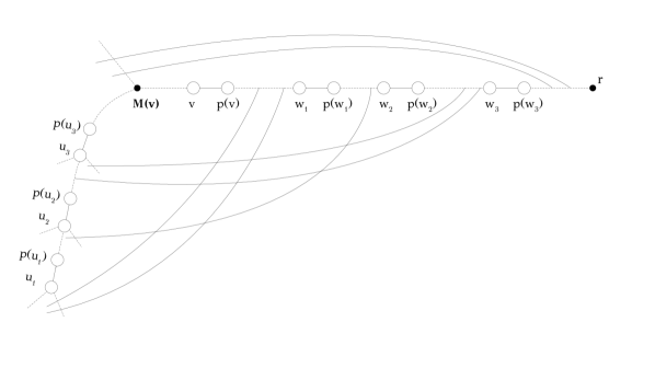
Figure 7: In this example we have $M(v)=M(w_{1})=M(w_{2})=M(w_{3})$, $U(v)=\{u_{1},u_{2},u_{3}\}$, and the triplets $\{(u_{i},p(u_{i})),(v,p(v)),(w_{i},p(w_{i}))\}$, for $i\in\{1,2,3\}$, are $3$-cuts. Observe that all $\{u_{1},u_{2},u_{3}\}$ are related as ancestor and descendant. This property is proved in Lemma 3.17. Furthermore, all $u\in U(v)$ have $\mathit{high}(u)=\mathit{high}(v)$.

Thus, $\mathit{stackU}[v]$ contains all $u$ that are predecessors of $v$ in $\mathit{high}^{-1}(\mathit{high}(v))$ and satisfy $\mathit{nextM}(u)=\emptyset$, $\mathit{low}(u)<\mathit{nextM}(v)$, $\mathit{low}(u)\geq\mathit{lastM}(v)$ and all elements of $\mathit{high}^{-1}(\mathit{high}(v))$ between $u$ and $v$ are ancestors of $u$. By Lemma 3.17, property $(1)$ of the stacks $\mathit{stackU}[v]$ is satisfied. The following lemma shows that property $(2)$ is also satisfied.

Lemma 3.18.

Let $v,v^{\prime}$ be two vertices such that $v^{\prime}$ is a proper ancestor of $v$ with $\mathit{high}(v^{\prime})=\mathit{high}(v)$, and let $u\in\mathit{stackU}[v]$. Then $u\notin\mathit{stackU}[v^{\prime}]$.

Proof.

First observe that the stacks $\mathit{stackU}[v]$ and $\mathit{stackU}[v^{\prime}]$ are non-empty only if $\mathit{nextM}(v)\neq\emptyset$ and $\mathit{nextM}(v^{\prime})\neq\emptyset$. Now, since $\mathit{high}(v^{\prime})=\mathit{high}(v)$, by Lemma 3.20, we have that $\mathit{nextM}(v)<\mathit{lastM}(v^{\prime})$. Since $u\in\mathit{stackU}[v]$, it has $\mathit{low}(u)<\mathit{nextM}(v)$. But then $\mathit{low}(u)<\mathit{lastM}(v^{\prime})$, and so $u\notin\mathit{stackU}[v^{\prime}]$. ∎

This implies that the total number of elements in all stacks $\mathit{stackU}[v]$ (by the time we have filled them) is $O(n)$. Now let $h$ be a vertex, and let us show how to fill the stacks $\mathit{stackU}[v]$, for all $v$ in the decreasingly sorted list $\mathit{high}^{-1}(h)$. To do this, we will need a stack $S$. We begin traversing the list $\mathit{high}^{-1}(h)$ from its first element, and when we process a vertex $u$ such that $\mathit{nextM}(u)=\emptyset$ we push it in $S$ if it is an ancestor of its predecessor (or the first elements of the list). Otherwise, we drop all elements from $S$, push $u$ in $S$, and keep traversing the list. When we meet a vertex $v$ that satisfies $\mathit{nextM}(v)\neq\emptyset$ and is also an ancestor of its predecessor, we check whether the top element $u$ of $S$ satisfies $\mathit{low}(u)<\mathit{lastM}(v)$, in which case we start popping elements out of $S$, until the top element $u$ of $S$ (if $S$ is not left empty) satisfies $\mathit{low}(u)\geq\mathit{lastM}(v)$. Then, as long as the top element $u$ of $S$ satisfies $\mathit{low}(u)<\mathit{nextM}(v)$, we repeatedly pop out the top element from $S$ and push it in $\mathit{stackU}[v]$. If $v$ is not an ancestor of its predecessor, we drop all elements from $S$. In any case, we keep traversing the list, following the same procedure, until we reach its end. This process is implemented in Algorithm 10. Property $(3)$ of the stacks $\mathit{stackU}$ is satisfied due to the way we fill them with this algorithm. To prove the correctness of Algorithm 10 - i.e., that by the time we reach the end of $\mathit{high}^{-1}(h)$, every stack $\mathit{stackU}[v]$, for every $v\in\mathit{high}^{-1}(h)$, contains all elements $u$ satisfying the necessary condition in Lemma 3.17 -, we need the following two lemmata.

Lemma 3.19.

If $u^{\prime}$ is an ancestor of $u$ with $\mathit{high}(u)=\mathit{high}(u^{\prime})$, then $\mathit{low}(u^{\prime})\leq\mathit{low}(u)$.

Proof.

Let $(x,y)\in B(u)$. Then $x$ is a descendant of $u$, and therefore a descendant of $u^{\prime}$. Furthermore, $y\leq\mathit{high}(u)=\mathit{high}(u^{\prime})$, and therefore $y$ is a proper ancestor of $u^{\prime}$. This shows that $(x,y)\in B(u^{\prime})$, and thus we have $B(u)\subseteq B(u^{\prime})$. $\mathit{low}(u^{\prime})\leq\mathit{low}(u)$ is an immediate consequence of this fact. ∎

Lemma 3.20.

Let $v,v^{\prime}$ be two vertices such that $v^{\prime}$ is a proper ancestor of $v$, $\mathit{nextM}(v)\neq\emptyset$, $\mathit{nextM}(v^{\prime})\neq\emptyset$, and $\mathit{high}(v^{\prime})=\mathit{high}(v)$. Then, $\mathit{nextM}(v)<\mathit{lastM}(v^{\prime})$.

Proof.

Let $(x,y)\in B(v)$. Then $x$ is a descendant of $v$, and therefore a descendant of $v^{\prime}$. Furthermore, since $y\leq\mathit{high}(v)$ and $\mathit{high}(v)=\mathit{high}(v^{\prime})$ and $\mathit{high}(v^{\prime})<v^{\prime}$, we have that $y$ is a proper ancestor of $v^{\prime}$. This shows that $(x,y)\in B(v^{\prime})$, and thus $B(v)\subseteq B(v^{\prime})$. From this we infer that $M(v)$ is a descendant of $M(v^{\prime})$. Now, since $M(\mathit{nextM}(v))=M(v)$ and $\mathit{nextM}(v)<v$, we have that $B(\mathit{nextM}(v))\subset B(v)$. This means that there exists a back-edge $(x,y)$ such that $x$ is a descendant of $M(v)$ and $y$ is a proper ancestor of $v$ but not a proper ancestor of $\mathit{nextM}(v)$. Then, since $(x,y)\in B(v)$, we have $y\leq\mathit{high}(v)$, and so $\mathit{high}(v)$ is not a proper ancestor of $\mathit{nextM}(v)$, and thus $\mathit{nextM}(v)$ is an ancestor of $\mathit{high}(v)$. Since $\mathit{high}(v)=\mathit{high}(v^{\prime})$ and $\mathit{high}(v^{\prime})$ is a proper ancestor of $v^{\prime}$, we infer that $\mathit{nextM}(v)$ is a proper ancestor of $v^{\prime}$. Now suppose, for the sake of contradiction, that $\mathit{lastM}(v^{\prime})$ is an ancestor of $\mathit{nextM}(v)$. Let $(x,y)\in B(\mathit{lastM}(v^{\prime}))$. Then, $x$ is a descendant of $M(\mathit{lastM}(v^{\prime}))$, and thus a descendant of $M(v^{\prime})$, and thus a descendant of $v^{\prime}$, and thus a descendant of $\mathit{nextM}(v)$. Furthermore, $y$ is a proper ancestor of $\mathit{lastM}(v^{\prime})$, and therefore a proper ancestor of $\mathit{nextM}(v)$. This shows that $(x,y)\in B(\mathit{nextM}(v))$, and thus we have $B(\mathit{lastM}(v^{\prime}))\subseteq B(\mathit{nextM}(v))$. From this we infer that $M(\mathit{lastM}(v^{\prime}))$ is a descendant of $M(\mathit{nextM}(v))$. But $M(\mathit{lastM}(v^{\prime}))=M(v^{\prime})$ and $M(\mathit{nextM}(v))=M(v)$. Thus, $M(v^{\prime})$ is a descendant of $M(v)$. Since $M(v)$ is a descendant of $M(v^{\prime})$, we conclude that $M(v^{\prime})=M(v)$. But this implies, in conjunction with $\mathit{high}(v^{\prime})=\mathit{high}(v)$, that $B(v)=B(v^{\prime})$, contradicting the fact that the graph is $3$-edge-connected. This shows that $\mathit{nextM}(v)$ is a proper ancestor of $\mathit{lastM}(v^{\prime})$. ∎

Now, to prove the correctness of Algorithm 10, we have to show that the elements we push into $\mathit{stackU}[v]$ satisfy the necessary condition in Lemma 3.17, and the elements we pop out from $S$ do not satisfy this condition either for $v$ or for any successor of $v$ in the list $\mathit{high}^{-1}(h)$. So, let $v$ be a vertex in $\mathit{high}^{-1}(h)$ such that $\mathit{nextM}(v)\neq\emptyset$, and let $v^{\prime}$ be a successor of $v$ in $\mathit{high}^{-1}(h)$ such that $\mathit{nextM}(v^{\prime})\neq\emptyset$. Now, when we meet $v$ as we traverse $\mathit{high}^{-1}(x)$, we pop out the top elements $u$ from $S$ that have $\mathit{low}(u)<\mathit{lastM}(v)$. By the definition of $\mathit{stackU}[v]$, these are not included in $\mathit{stackU}[v]$. Now, by Lemma 3.20, we have $\mathit{nextM}(v)<\mathit{lastM}(v^{\prime})$. Since $\mathit{low}(u)<\mathit{lastM}(v)\leq\mathit{nextM}(v)$, we have $\mathit{low}(u)<\mathit{lastM}(v^{\prime})$, and thus $u$ is not in $\mathit{stackU}[v^{\prime}]$ either, so it does not matter that we pop those $u$ out of $S$. Then, once we reach a $\tilde{u}$ in $S$ that satisfies $\mathit{low}(\tilde{u})\geq\mathit{lastM}(v)$, we pop out the top elements $u$ of $S$ that have $\mathit{low}(u)<\mathit{nextM}(v)$, and push them into $\mathit{stackU}[v]$. This is according to the definition of $\mathit{stackU}[v]$. Since $\mathit{nextM}(v)<\mathit{lastM}(v^{\prime})$ and $\mathit{low}(u)<\mathit{nextM}(v)$, we have $\mathit{low}(u)<\mathit{lastM}(v^{\prime})$, and so, again, these $u$ are not included in $\mathit{stackU}[v^{\prime}]$, and thus it does not matter that we pop them out of $S$. Now, when we reach a $u$ in $S$ that has $\mathit{low}(u)\geq\mathit{nextM}(v)$, we can be certain, by Lemma 3.19, that no $u^{\prime}$ in $S$ has $\mathit{low}(u^{\prime})<\mathit{nextM}(v)$, since all elements of $S$ are descendants of $u$ (by the way we fill the stack $S$), and thus they have $\mathit{low}(u^{\prime})\geq\mathit{low}(u)\geq\mathit{nextM}(v)$. Then it is proper to move on to the next element of $\mathit{high}^{-1}(h)$.

1 initialize a stack $S$

2 foreach vertex $v$ do initialize a stack $\mathit{stackU}[v]$

3 foreach vertex $h$ do

4       $u\leftarrow$ first element of $\mathit{high}^{-1}(h)$

5       while $u\neq\emptyset$ do

6             $z\leftarrow$ next element of $\mathit{high}^{-1}(h)$

7             if $z=\emptyset$ then break

8             if $z$ is not an ancestor of $u$ then

9                   pop out all elements from $S$

10                  

11             end if

12            if $\mathit{nextM}(z)=\emptyset$ then

13                   $S$.push($z$)

14                  

15             end if

16            else if $\mathit{nextM}(z)\neq\emptyset$ then

17                   while $\mathit{low}(S\mathit{.top()})<\mathit{lastM}(v)$ do $S$.pop()

18                   while $\mathit{low}(S\mathit{.top()})<\mathit{nextM}(v)$ do

19                         $u\leftarrow S$.pop()

20                         $\mathit{stackU}[v]$.push($u$)

21                        

22                   end while

23                  

24             end if

25            $u\leftarrow z$

26            

27       end while

28      

29 end foreach

Algorithm 10 Fill all stacks $\mathit{stackU}[v]$, for all vertices $v$

Lemma 3.21.

Let $v$ be a vertex and $u,u^{\prime}$ two elements in $\mathit{stackU}[v]$, where $u$ is a predecessor of $u^{\prime}$ in $\mathit{stackU}[v]$. Then, $\mathit{low}(u^{\prime})\leq\mathit{low}(u)$.

Proof.

Since $u,u^{\prime}\in\mathit{stackU}[v]$, we have $\mathit{high}(u)=\mathit{high}(v)=\mathit{high}(u^{\prime})$. Since $u$ is a predecessor of $u^{\prime}$ in $\mathit{stackU}[v]$, by property $(3)$ of $\mathit{stackU}[v]$ we have that $u$ is a descendant of $u^{\prime}$. Thus, by Lemma 3.19, we get $\mathit{low}(u^{\prime})\leq\mathit{low}(u)$. ∎

The next lemma is the basis to find all $3$-cuts of the form $\{(u,p(u)),(v,p(v)),(w,p(w))\}$, where $u$ is a descendant of $v$, $M(v)=M(w)$, and $w\neq\mathit{nextM}(v)$.

Lemma 3.22.

Let $u$ be a vertex in $\mathit{stackU}[v]$ and $w$ a proper ancestor of $v$ such that $M(w)=M(v)$. Then, if $\{(u,p(u)),(v,p(v)),(w,p(w))\}$ is a $3$-cut, we have that $\mathit{b\_count}(v)=\mathit{b\_count}(u)+\mathit{b\_count}(w)$ and $w$ is the greatest element of $M^{-1}(M(v))$ such that $w\leq\mathit{low}(u)$. Conversely, if $\mathit{b\_count}(v)=\mathit{b\_count}(u)+\mathit{b\_count}(w)$ and $w\leq\mathit{low}(u)$, then $\{(u,p(u)),(v,p(v)),(w,p(w))\}$ is a $3$-cut.

Proof.

($\Rightarrow$) By proposition 3.12, we have $B(v)=B(u)\sqcup B(w)$. This explains both $\mathit{b\_count}(v)=\mathit{b\_count}(u)+\mathit{b\_count}(w)$ and $w\leq\mathit{low}(u)$. (For if we had $\mathit{low}(u)<w$, then, since $u$ is a descendant of $w$, $B(u)$ would meet $B(w)$.) Now suppose, for the sake of contradiction, that there is a vertex $w^{\prime}$ such that $M(w^{\prime})=M(v)$ and $w<w^{\prime}\leq\mathit{low}(u)$. Since $B(v)=B(u)\sqcup B(w)$, we have that $\mathit{low}(u)<v$, and therefore $w^{\prime}<v$. Since $M(w^{\prime})=M(v)$, this means that $B(w^{\prime})\subset B(v)$. Furthermore, since $M(w)=M(w^{\prime})$ and $w<w^{\prime}$, we infer that $B(w)\subset B(w^{\prime})$, and therefore there exists a back-edge $(x,y)\in B(w^{\prime})\setminus B(w)$. Then, by $B(w^{\prime})\subset B(v)$, we have that $(x,y)\in B(v)$, and $B(v)=B(u)\sqcup B(w)$ implies that $(x,y)\in B(u)$ or $(x,y)\in B(w)$. Since $(x,y)\notin B(w)$, $(x,y)\in B(u)$ is the only option left. But $y$ is a proper ancestor of $w^{\prime}$, and therefore a proper ancestor of $\mathit{low}(u)$ (since $w^{\prime}\leq\mathit{low}(u)$). This implies that $(x,y)\notin B(u)$, which is absurd. We conclude that $w$ is the greatest element of $M^{-1}(M(v))$ such that $w\leq\mathit{low}(u)$.
($\Leftarrow$) By proposition 3.12, is is sufficient to show that $B(v)=B(u)\sqcup B(w)$. $u\in\mathit{stackU}[v]$ implies that $u$ is a descendant of $v$ such that $\mathit{high}(u)=\mathit{high}(v)$. Now let $(x,y)\in B(u)$. Then $x$ is a descendant of $u$, and therefore a descendant of $v$. Furthermore, $y\leq\mathit{high}(u)=\mathit{high}(v)$, and therefore $y$ is a proper ancestor of $v$. This shows that $(x,y)\in B(v)$, and thus we have $B(u)\subseteq B(v)$. Since $M(w)=M(v)$ and $w<v$, we have $B(w)\subset B(v)$. Thus we have established that $B(u)\cup B(w)\subseteq B(v)$. Notice that no $(x,y)\in B(u)$ is contained in $B(w)$, since $y\geq\mathit{low}(u)\geq w$, and thus $y$ is not a proper ancestor of $w$. Thus we have $B(u)\cap B(w)=\emptyset$. Now $B(v)=B(u)\sqcup B(w)$ follows from $B(u)\cup B(w)\subseteq B(v)$, $B(u)\cap B(w)=\emptyset$ and $\mathit{b\_count}(v)=\mathit{b\_count}(u)+\mathit{b\_count}(w)$. ∎

Now our goal is to find, for every $u\in\mathit{stackU}[v]$, for every vertex $v$, the vertex $w$ (if it exists) which has $M(w)=M(v)$ and $w<\mathit{nextM}(v)$, and is such that $\{(u,p(u)),(v,p(v)),(w,p(w))\}$ is a $3$-cut. By Lemma 3.22, $w$ has the property that it is the greatest vertex in $M^{-1}(M(v))$ which has $w\leq\mathit{low}(u)$. Let us describe a simple method to find the $w$ with this property, which will give us the intuition to provide a linear-time algorithm for our problem. So let $v$ be a vertex, $m=M(v)$, and $u$ be a vertex in $\mathit{stackU}[v]$. A simple idea is to start from $v$ and keep traversing the list $M^{-1}(m)$, through the pointers $\mathit{nextM}$, until we reach a $w\in M^{-1}(m)$ such that $w\leq\mathit{low}(u)$. The problem here is that we may have to pass from the same elements of $M^{-1}(m)$ an excessive amount of times (depending on the number of elements in $\mathit{stackU}[v]$). We can remedy this by keeping in a variable $\mathit{lowestW}$ the $w$ that we reached the last time we processed a $u\in\mathit{stackU}[v]$. Then, when we process the successor of $u$ in $\mathit{stackU}[v]$, we begin the search in $M^{-1}(m)$ from $\mathit{lowestW}$. This will work, since the every $u\in\mathit{stackU}[v]$ is a descendant of its successor $u^{\prime}$ in $\mathit{stackU}[v]$ (due to the way we have filled the stacks $\mathit{stackU}$ with Algorithm 10), and we have $\mathit{high}(u)=\mathit{high}(u^{\prime})$, and therefore, by Lemma 3.19, $\mathit{low}(u^{\prime})\leq\mathit{low}(u)$. However, this is, again, not a linear-time procedure, since, for every vertex $v$, when we start processing the first vertex in $\mathit{stackU}[v]$, we begin traversing the list $M^{-1}(M(v))$ from $v$, and therefore, every time we process a vertex $v^{\prime}$ with $M(v^{\prime})=M(v)$, we may have to pass again from the same vertices that we passed from during the processing of $v$, exceeding the time bound in total. Now, to achieve linear time, we process the vertices from the lowest to the highest, and, for every $v$ that we process, we keep in a variable $\mathit{lowestW}[v]$ the $w$ that we reached the last time we processed a $u\in\mathit{stackU}[v]$. Then, when we have to process a $u\in\mathit{stackU}[v]$, we traverse the list $M^{-1}(M(v))$ through the pointers $\mathit{lowestW}$, starting from $\mathit{lowestW}[v]$. (Initially, we set every $\mathit{lowestW}[v]$ to $\mathit{nextM}(v)$.) Thus we perform a kind of path-compression method, which is shown Algorithm 11. The next three lemmata will be used in proving the correctness and linear complexity of Algorithm 11.

Lemma 3.23.

Let $v$ be a vertex and $u\in\mathit{stackU}[v]$. When we reach line 11 during the processing of $u$, we have that $w$ is a vertex in $M^{-1}(M(v))$ such that $w\leq\mathit{low}(u)$ and $w\leq\mathit{min}\{\mathit{low}(u^{\prime})\mid\exists v^{\prime}\mbox{ with }M(v^{\prime})=M(v)\mbox{, }w<v^{\prime}<v\mbox{ and }u^{\prime}\in\mathit{stackU}[v^{\prime}]\}$.

Proof.

First observe that, during the processing of a vertex $v$, the variables $w$ and $\mathit{lowestW}[v]$ are members of $M^{-1}(M(v))$, and $w$ is an ancestor of $v$ while $\mathit{lowestW}[v]$ is a proper ancestor of $v$. (It is easy to see this inductively. For if this holds for all vertices $v^{\prime}<v$, then it is also true for $v$, since the while loop in line 11 assigns $w$ to $\mathit{lowestW}[w]$, and $w$ is assumed to be an ancestor of $v$ with $M(w)=M(v)$, and thus $\mathit{lowestW}[w]$ is also an ancestor of $v$ with $M(\mathit{lowestW}[w])=M(v)$, due to the inductive hypothesis.) Then it is obvious that, when we reach line 11 during the processing of $u\in\mathit{stackU}[v]$, we have that $M(w)=M(v)$ and $w\leq\mathit{low}(u)$, since the while loop in line 11 terminates precisely when such a $w$ is found. Now we will show that, when we process a $u\in\mathit{stackU}[v]$, every time $w$ is assigned $\mathit{lowestW}[w]$ during the execution of the while loop in line 11, we have $w\leq\mathit{low}(u^{\prime})$, for every $u^{\prime}\in\mathit{stackU}[v^{\prime}]$, for every $v^{\prime}$ with $M(v^{\prime})=M(v)$ and $w<v^{\prime}<v$. It is easy to see this inductively. Suppose, then, that this was the case for every vertex that we processed before $v$, for every predecessor of $u$ in $\mathit{stackU}[v]$ that we already processed, and for every step of the while loop in line 11 in the processing of $u$ so far. Thus, now $w$ has the property that $w\leq\mathit{low}(u^{\prime})$, for every $u^{\prime}\in\mathit{stackU}[v^{\prime}]$, for every $v^{\prime}$ with $M(v^{\prime})=M(v)$ and $w<v^{\prime}<v$. So let us perform $w\leftarrow\mathit{lowestW}[w]$ once more (which means that we still have $w>\mathit{low}(u)$), and let $\tilde{w}$ be the current value of $w$, to distinguish it from the previous one which we will denote simply as $w$. Now, due to the inductive hypothesis, we have that $\tilde{w}\leq\mathit{low}(u^{\prime})$ for every $u^{\prime}\in\mathit{stackU}[v^{\prime}]$, for every $v^{\prime}$ with $M(v^{\prime})=M(v)$ and $\tilde{w}<v^{\prime}<w$. We also have (again, due to the inductive hypothesis) that $w\leq\mathit{low}(u^{\prime})$ for every $u^{\prime}\in\mathit{stackU}[v^{\prime}]$, for every $v^{\prime}$ with $M(v^{\prime})=M(v)$ and $w<v^{\prime}<v$. Since $\tilde{w}<w$, we thus have $\tilde{w}\leq\mathit{low}(u^{\prime})$, for every $u^{\prime}\in\mathit{stackU}[v^{\prime}]$, for every $v^{\prime}$ with $M(v^{\prime})=M(v)$ and $\tilde{w}<v^{\prime}<w$ or $w<v^{\prime}<v$. Thus we only have to consider the case $v^{\prime}=w$, and prove that every $u^{\prime}\in\mathit{stackU}[w]$ satisfies $\tilde{w}\leq\mathit{low}(u^{\prime})$. Observe that $\mathit{lowestW}[w]$ was updated for the last time in line 11 when we were processing the last element $\tilde{u}$ of $\mathit{stackU}[w]$. Then, since $\tilde{w}=\mathit{lowestW}[w]$, due to the inductive hypothesis we have that $\tilde{w}\leq\mathit{low}(\tilde{u})$. Since every $u^{\prime}\in\mathit{stackU}[w]$ has $\mathit{high}(u^{\prime})=\mathit{high}(\tilde{u})$ and $\tilde{u}$ is an ancestor of its predecessors in $\mathit{stackU}[w]$ (due to the way we have filled the stacks $\mathit{stackU}$ with Algorithm 10), by Lemma 3.19 we have that $\mathit{low}(\tilde{u})\leq\mathit{low}(u^{\prime})$, and therefore $\tilde{w}\leq\mathit{low}(u^{\prime})$. Thus we have shown that $\tilde{w}\leq\mathit{low}(u^{\prime})$, for every $u^{\prime}\in\mathit{stackU}[v^{\prime}]$, for every $v^{\prime}$ with $M(v^{\prime})=M(v)$ and $\tilde{w}<v^{\prime}<v$. ∎

Lemma 3.24.

Let $v$ be a vertex and $u\in\mathit{stackU}[v]$. When we reach line 11 during the processing of $u$, we have that $w$ is the greatest vertex in $M^{-1}(M(v))$ such that $w\leq\mathit{low}(u)$ and $w\leq\mathit{min}\{\mathit{low}(u^{\prime})\mid\exists v^{\prime}\mbox{ with }M(v^{\prime})=M(v)\mbox{, }w<v^{\prime}<v\mbox{ and }u^{\prime}\in\mathit{stackU}[v^{\prime}]\}$.

Proof.

We will prove this lemma by induction. Let’s assume, then, that, for every vertex $v^{\prime}\leq v$, and every $u^{\prime}\in\mathit{stackU}[v^{\prime}]$ that we processed so far, whenever we reached line 11 $w$ was the greatest vertex with $M(w)=M(v^{\prime})$ such that $w\leq\mathit{low}(u)$ and $w\leq\mathit{min}\{\mathit{low}(u^{\prime\prime})\mid\exists v^{\prime\prime}\mbox{ with }M(v^{\prime\prime})=M(v^{\prime})\mbox{, }w<v^{\prime\prime}<v^{\prime}\mbox{ and }u^{\prime\prime}\in\mathit{stackU}[v^{\prime\prime}]\}$. Now let $u$ be the next element of $\mathit{stackU}[v]$ that we process. Let $\tilde{w}$ be the greatest vertex with $M(\tilde{w})=M(v)$ such that $\tilde{w}\leq\mathit{low}(u)$ and $\tilde{w}\leq\mathit{min}\{\mathit{low}(u^{\prime})\mid\exists v^{\prime}\mbox{ with }M(v^{\prime})=M(v)\mbox{, }\tilde{w}<v^{\prime}<v\mbox{ and }u^{\prime}\in\mathit{stackU}[v^{\prime}]\}$. (The existence of such a $\tilde{w}$ is guaranteed by Lemma 3.23.) Let $w$ be the last vertex during the execution of the while loop in line 11 that had $w>\mathit{low}(u)$, and let $w^{\prime}=\mathit{lowestW}[w]$. Then we have that $w^{\prime}=\mathit{lowestW}[w]\leq\mathit{low}(u)$, and the while loop terminates here. We will show that $w^{\prime}=\tilde{w}$. We distinguish two cases, depending on whether $w^{\prime}=\mathit{nextM}(w)$ or $w^{\prime}\neq\mathit{nextM}(w)$. In the first case, we have that $w>\mathit{low}(u)$, but $\mathit{nextM}(w)\leq\mathit{low}(u)$. Thus, $w^{\prime}=\mathit{nextM}(w)$ is the greatest vertex with $M(w^{\prime})=M(v)$ such that $w^{\prime}\leq\mathit{low}(u)$, and so we have $w^{\prime}=\tilde{w}$ (since $w^{\prime}$ satisfies also $w^{\prime}\leq\mathit{min}\{\mathit{low}(u^{\prime})\mid\exists v^{\prime}\mbox{ with }M(v^{\prime})=M(v)\mbox{, }w<v^{\prime}<v\mbox{ and }u^{\prime}\in\mathit{stackU}[v^{\prime}]\}$, by Lemma 3.23). Now, if $w^{\prime}\neq\mathit{nextM}(w)$, this means, due to the inductive hypothesis (and since $w^{\prime}=\mathit{lowestW}[w]$), that $w^{\prime}$ is the greatest vertex with $M(w^{\prime})=M(w)$ such that $w^{\prime}\leq\mathit{low}(\tilde{u})$ and $w^{\prime}\leq\mathit{min}\{\mathit{low}(u^{\prime})\mid\exists v^{\prime}\mbox{ with }M(v^{\prime})=M(w)\mbox{, }w^{\prime}<v^{\prime}<w\mbox{ and }u^{\prime}\in\mathit{stackU}[v^{\prime}]\}$, where $\tilde{u}$ is the last element in $\mathit{stackU}[w]$. Now, since $\tilde{w}$ satisfies $\tilde{w}\leq\mathit{min}\{\mathit{low}(u^{\prime})\mid\exists v^{\prime}\mbox{ with }M(v^{\prime})=M(v)\mbox{, }\tilde{w}<v^{\prime}<v\mbox{ and }u^{\prime}\in\mathit{stackU}[v^{\prime}]\}$ and $\tilde{w}<w<v$, we have $\tilde{w}\leq\mathit{low}(\tilde{u})$ and $\tilde{w}\leq\mathit{min}\{\mathit{low}(u^{\prime})\mid\exists v^{\prime}\mbox{ with }M(v^{\prime})=M(w)\mbox{, }\tilde{w}<v^{\prime}<w\mbox{ and }u^{\prime}\in\mathit{stackU}[v^{\prime}]\}$. Thus, $\tilde{w}$ cannot be greater than $w^{\prime}$, and so we have $w^{\prime}\geq\tilde{w}$. Since $w^{\prime}\leq\mathit{low}(u)$, and, as a consequence of Lemma 3.23, $w^{\prime}\leq\mathit{min}\{\mathit{low}(u^{\prime})\mid\exists v^{\prime}\mbox{ with }M(v^{\prime})=M(v)\mbox{, }w^{\prime}<v^{\prime}<v\mbox{ and }u^{\prime}\in\mathit{stackU}[v^{\prime}]\}$, it must be the case that $w^{\prime}=\tilde{w}$. ∎

Lemma 3.25.

Let $\{(u,p(u)),(v,p(v)),(w,p(w))\}$ be a $3$-cut where $u$ is a descendant of $v$, $v$ is a descendant of $w$ with $M(v)=M(w)$, and $w\neq\mathit{nextM}(v)$. Then, $w$ is the greatest vertex in $M^{-1}(M(v))$ such that $w\leq\mathit{low}(u)$ and $w\leq\mathit{min}\{\mathit{low}(u^{\prime})\mid\exists v^{\prime}\mbox{ with }M(v^{\prime})=M(v)\mbox{, }w<v^{\prime}<v\mbox{ and }u^{\prime}\in\mathit{stackU}[v^{\prime}]\}$.

Proof.

Suppose, for the sake of contradiction, that there exists a vertex $v^{\prime}$ with $M(v^{\prime})=M(v)$ and $w<v^{\prime}<v$, such that there exists a $u^{\prime}\in\mathit{stackU}[v^{\prime}]$ with $\mathit{low}(u^{\prime})<w$. Since $u^{\prime}\in\mathit{stackU}[v^{\prime}]$, we have that $u^{\prime}$ is a proper descendant of $v^{\prime}$ with $\mathit{high}(u^{\prime})=\mathit{high}(v^{\prime})$. Let $(x,y)\in B(u^{\prime})$ (of course, $B(u^{\prime})$ is not empty, since the graph is $3$-edge-connected). Then $x$ is a descendant of $u^{\prime}$, and therefore a descendant of $v^{\prime}$. Furthermore, $y\leq\mathit{high}(u^{\prime})=\mathit{high}(v^{\prime})$, and therefore $y$ is a proper ancestor of $v^{\prime}$. This shows that $(x,y)\in B(v^{\prime})$. Thus we have $B(u^{\prime})\subset B(v^{\prime})$. Since $M(v^{\prime})=M(v)$ and $v^{\prime}<v$, we have $B(v^{\prime})\subset B(v)$. Thus, $B(u^{\prime})\subset B(v)$. Now we will prove that $u^{\prime}$ is not related as ancestor or descendant with $u$. First, since $\mathit{low}(u^{\prime})<w\leq\mathit{low}(u)$, it cannot be the case that $u^{\prime}$ is a descendant of $u$ (for a back-edge $(x,\mathit{low}(u^{\prime}))\in B(u^{\prime})$ would also be a back-edge in $B(u)$, and thus we would have $\mathit{low}(u)\leq\mathit{low}(u^{\prime})$, which is a absurd). Suppose, then, that $u^{\prime}$ is an ancestor of $u$. Since $v^{\prime}$ is a proper ancestor of $v$ with $M(v^{\prime})=M(v)$, we must have $\mathit{high}(v^{\prime})<\mathit{high}(v)$; and since $\mathit{high}(u^{\prime})=\mathit{high}(v^{\prime})$, we therefore have $\mathit{high}(u^{\prime})<\mathit{high}(v)$. This means that $u^{\prime}$ (which is related as ancestor or descendant with $v$, since we supposed it is an ancestor of $u$) is a proper ancestor of $v$, and therefore a proper ancestor of $M(v)$. Since, then, $u^{\prime}$ is a descendant $v^{\prime}$ and $M(v^{\prime})=M(v)$, by Lemma 2.4 we have that $M(u^{\prime})$ is an ancestor of $M(v)$. But $B(u^{\prime})\subset B(v)$ implies that $M(u^{\prime})$ is a descendant of $M(v)$, and therefore $M(u^{\prime})=M(v)$. Since $M(v)=M(v^{\prime})$ and $\mathit{high}(v^{\prime})=\mathit{high}(u^{\prime})$, we get that $B(u^{\prime})=B(v^{\prime})$, which implies that $v^{\prime}=u^{\prime}$ - a contradiction. Thus we have shown that $u^{\prime}$ is not related as ancestor or descendant with $u$.

Now let $(x,y)$, with $y=\mathit{high}(u^{\prime})$, be a back-edge in $B(u^{\prime})$. Then we have $(x,y)\in B(v)$. By proposition 3.12, we have $B(v)=B(u)\sqcup B(w)$, and therefore $(x,y)\in B(u)$ or $(x,y)\in B(w)$. Since $u^{\prime}$ is not related as ancestor of descendant with $u$, it cannot be the case that $x$ (which is a descendant of $u^{\prime}$) is a descendant of $u$, and therefore $(x,y)\in B(u)$ is rejected. Now, since $B(u^{\prime})\subset B(v^{\prime})$, we have $(x,y)\in B(v^{\prime})$. Since $M(v^{\prime})=M(w)$ and $w<v^{\prime}$, we have that $B(w)\subset B(v^{\prime})$, and thus there exists a back-edge $(x^{\prime},y^{\prime})\in B(v^{\prime})$ such that $y^{\prime}\in T(v^{\prime},w]$. But since $y=\mathit{high}(u^{\prime})=\mathit{high}(v^{\prime})$, we must have $y^{\prime}\leq y$. Thus, $y$ is not a proper ancestor of $w$, and so $(x,y)\notin B(w)$, either. We have arrived at a contradiction, as a consequence of our initial supposition. This shows that there is no vertex $v^{\prime}$ with $M(v^{\prime})=M(v)$ and $w<v^{\prime}<v$, such that there exists a $u^{\prime}\in\mathit{stackU}[v^{\prime}]$ with $\mathit{low}(u^{\prime})<w$. Thus, $w\leq\mathit{min}\{\mathit{low}(u^{\prime})\mid\exists v^{\prime}\mbox{ with }M(v^{\prime})=M(v)\mbox{, }w<v^{\prime}<v\mbox{ and }u^{\prime}\in\mathit{stackU}[v^{\prime}]\}$. Now, by Lemma 3.22, $w$ is the greatest vertex in $M^{-1}(M(v))$ with $w\leq\mathit{low}(u)$. Thus, $w$ must be the greatest vertex in $M^{-1}(M(v))$ that satisfies both $w\leq\mathit{low}(u)$ and $w\leq\mathit{min}\{\mathit{low}(u^{\prime})\mid\exists v^{\prime}\mbox{ with }M(v^{\prime})=M(v)\mbox{, }w<v^{\prime}<v\mbox{ and }u^{\prime}\in\mathit{stackU}[v^{\prime}]\}$. ∎

1 initialize an array $\mathit{lowestW}$ with $n$ entries

2 foreach vertex $v$ do $\mathit{lowestW}[v]\leftarrow\mathit{nextM}(v)$

3 for $v\leftarrow 1$ to $v\leftarrow n$ do

4       while $\mathit{stackU}[v]\mathit{.top()}\neq\emptyset$ do

5             $u\leftarrow\mathit{stackU}[v]$.pop()

6             $w\leftarrow\mathit{lowestW}[v]$

7             while $w>\mathit{low}(u)$ do $w\leftarrow\mathit{lowestW}[w]$

8             $\mathit{lowestW}[v]\leftarrow w$

9             if $\mathit{b\_count}(v)=\mathit{b\_count}(u)+\mathit{b\_count}(w)$ then

10                   mark the triplet $\{(u,p(u)),(v,p(v)),(w,p(w))\}$

11                  

12             end if

13            

14       end while

15      

16 end for

Algorithm 11 Find all $3$-cuts $\{(u,p(u)),(v,p(v)),(w,p(w))\}$, where $u$ is a descendant of $v$, $v$ is a descendant of $w$ with $M(v)=M(w)$, and $w\neq\mathit{nextM}(v)$.

Proposition 3.26.

Algorithm 11 identifies all $3$-cuts $\{(u,p(u)),(v,p(v)),(w,p(w))\}$, where $u$ is a descendant of $v$, $v$ is a descendant of $w$ with $M(v)=M(w)$, and $w\neq\mathit{nextM}(v)$. Furthermore, it runs in linear time.

Proof.

Let $\{(u,p(u)),(v,p(v)),(w,p(w))\}$ be a $3$-cut, where $u$ is a descendant of $v$, $v$ is a descendant of $w$ with $M(v)=M(w)$, and $w\neq\mathit{nextM}(v)$. By Lemma 3.25, $w$ is the greatest vertex in $M^{-1}(M(v))$ such that $w\leq\mathit{low}(u)$ and $w\leq\mathit{min}\{\mathit{low}(u^{\prime})\mid\exists v^{\prime}\mbox{ with }M(v^{\prime})=M(v)\mbox{, }w<v^{\prime}<v\mbox{ and }u^{\prime}\in\mathit{stackU}[v^{\prime}]\}$. By Lemma 3.24, Algorithm 11 will identify $w$ during the processing of $u$ in line 11. As a consequence of proposition 3.12, we have $\mathit{b\_count}(v)=\mathit{b\_count}(u)+\mathit{b\_count}(w)$, and thus the triplet $\{(u,p(u)),(v,p(v)),(w,p(w))\}$ will be marked in line 11. Conversely, let $\{(u,p(u)),(v,p(v)),(w,p(w))\}$ be a triplet that gets marked by Algorithm 11 in line 11. Then, we have $u\in\mathit{stackU}[v]$. Furthermore, Lemma 3.24 implies that $w$ has $M(w)=M(v)$ and $w\leq\mathit{low}(u)$. Then, since $u\in\mathit{stackU}[v]$, we have $\mathit{low}(u)<\mathit{nextM}(v)$, and therefore $w$ is a proper ancestor of $v$. Now, since $\mathit{b\_count}(v)=\mathit{b\_count}(u)+\mathit{b\_count}(w)$, Lemma 3.22 implies that $\{(u,p(u)),(v,p(v)),(w,p(w))\}$ is a $3$-cut. Thus, the correctness of Algorithm 11 is established.

To prove that Algorithm 11 runs in linear time, we will count the number of times that we access the array $\mathit{lowestW}$ during the while loop in line 11. Specifically, we will show that, by the time the algorithm is terminated, the $v$ entry of $\mathit{lowestW}$, for every vertex $v$, will have been accessed at most once in line 11. We will prove this inductively, using the inductive proposition: $\Pi(v)\equiv$ after processing $v$, we have that $\forall v^{\prime}<v$ $\mathit{lowestW}[v^{\prime}]$ has been accessed at most once in line 11 during the course of the algorithm so far and $\forall v^{\prime}\leq v$ we have that every $w\in T(v^{\prime},\mathit{lowestW}[v^{\prime}])$ has $\mathit{lowestW}[w]\geq\mathit{lowestW}[v^{\prime}]$. Thus, (the first part of) $\Pi(n)$ implies the linearity of Algorithm 11. Now, suppose that $\Pi(v-1)$ is true for a $v\in\{1,\dotsc,n\}$ (observe that $\Pi(0)$ is trivially true). We will prove that $\Pi(v)$ is also true. Thus we have to show that: after we have processed every $u\in\mathit{stackU}[v]$, we have that $\forall v^{\prime}<v$ $\mathit{lowestW}[v^{\prime}]$ has been accessed at most once in line 11 during the course of the algorithm so far and $\forall v^{\prime}\leq v$ we have that every $w\in T(v^{\prime},\mathit{lowestW}[v^{\prime}])$ has $\mathit{lowestW}[w]\geq\mathit{lowestW}[v^{\prime}]$ $(1)$. Now, suppose that this was a case for a specific $\tilde{u}\in\mathit{stackU}[v]$. We will show that it is still true for the successor $u$ of $\tilde{u}$ in $\mathit{stackU}[v]$. (Of course, due to the inductive hypothesis, $(1)$ is definitely true before we have began processing the elements of $\mathit{stackU}[v]$, and therefore we may also have that $u$ is the first element of $\mathit{stackU}[v]$ in what follows.) Let $\tilde{w}$ be the value of $\mathit{lowestW}[v]$ after the assignment in line 11, during the processing of $u$. Thus, all vertices that we traversed during the execution of the while loop, during the processing of $u$, are contained in $T[v,\tilde{w}]$. Now let $v^{\prime}<v$ be a vertex with the property that $\mathit{lowestW}[v^{\prime}]$ has been accessed once in line 11 during the course of the algorithm before the processing of $u$, and let $\tilde{v}$ be the vertex during whose processing we had to access $\mathit{lowestW}[v^{\prime}]$ in the while loop. We will show that $\mathit{lowestW}[v^{\prime}]$ will not be accessed in line 11 during the processing of $u$. Of course, we may assume that $v^{\prime}$ is in $T[v,\tilde{w})$, for otherwise it is clear that the $v^{\prime}$ entry of $\mathit{lowestW}$ will not be accessed during the execution of the while loop (since the traversal in while loop will not reach vertices lower than $\tilde{w}$, and when it reaches $\tilde{w}$ it will terminate). We note that, since the $v^{\prime}$ entry of $\mathit{lowestW}$ was accessed during the execution of the while loop during the processing of $\tilde{v}$, we have that $\mathit{lowestW}[\tilde{v}]$ is an ancestor of $\mathit{lowestW}[v^{\prime}]$, and therefore a proper ancestor of $v^{\prime}$. Now, if $\tilde{v}=v$, then $\mathit{lowestW}[v]$ was assigned $\mathit{lowestW}[\tilde{v}]$, in line 11, during the processing of a predecessor of $u$ in $\mathit{stackU}[v]$. Thus, when we begin processing $u$, $w$ is assigned a proper ancestor of $v^{\prime}$ in line 11, before entering the while loop, and so the $v^{\prime}$ entry of $\mathit{lowestW}$ will not be accessed during the execution of the while loop. So let’s assume that $\tilde{v}<v$. Initially, the variable $w$ is assigned $\mathit{lowestW}[v]$ in line 11. We claim that $\mathit{lowestW}[v]$ is either a descendant of $\tilde{v}$ or a proper ancestor of $v^{\prime}$. To see this, suppose, for the sake of contradiction, that $\mathit{lowestW}[v]$ is in $T(\tilde{v},v^{\prime}]$. Then, we have $\tilde{v}\in T(v,\mathit{lowestW}[v])$, and therefore, since $(1)$ is true for $\tilde{u}$ (the predecessor of $u$ in $\mathit{stackU}[v]$), we have that $\mathit{lowestW}[\tilde{v}]\geq\mathit{lowestW}[v]$. Since $\mathit{lowestW}[\tilde{v}]$ is a proper ancestor of $v^{\prime}$, this implies that $v^{\prime}>\mathit{lowestW}[v]$, contradicting the supposition $\mathit{lowestW}[v]\leq v^{\prime}$. Thus, before executing the while loop, we have that $w$ is either a descendant of $\tilde{v}$ or a proper ancestor of $v^{\prime}$. Now suppose that the while loop has been executed $0$ or more times, and $w$ is assigned a descendant of $\tilde{v}$ or a proper ancestor of $v^{\prime}$. We will show that if we execute the while loop once more, $w$ will either be assigned a descendant of $\tilde{v}$ or a proper ancestor of $v^{\prime}$. Of course, if $w$ is a proper ancestor of $v^{\prime}$, the same is true for $\mathit{lowestW}[w]$. Moreover, if $w=\tilde{v}$, then, as noted above, we have that $\mathit{lowestW}[w]$ is a proper ancestor of $v^{\prime}$. So let’s assume that $w$ is a proper descendant of $\tilde{v}$, and suppose, for the sake of contradiction, that $\mathit{lowestW}[w]$ is in $T(\tilde{v},v^{\prime}]$. Then, since $\tilde{v}\in T(w,\mathit{lowest}[w])$, due to the inductive hypothesis we have that $\mathit{lowestW}[\tilde{v}]\geq\mathit{lowestW}[w]$. Since we also have $v^{\prime}>\mathit{lowestW}[\tilde{v}]$, this contradicts the supposition $\mathit{lowestW}[w]\geq v^{\prime}$. Thus, if $w$ is a proper descendant of $\tilde{v}$, $\mathit{lowestW}[w]$ is either a descendant of $\tilde{v}$ or a proper ancestor of $v^{\prime}$. In any case, then, during the execution of the while loop, $w$ will be assigned either a descendant of $\tilde{v}$ or a proper ancestor of $v^{\prime}$, and thus the $v^{\prime}$ entry of $\mathit{lowestW}$ will not be accessed.

It remains to show that, after the processing of $u$, for every $w\in T(v,\tilde{w})$ we have $\mathit{lowestW}[w]\geq\tilde{w}$. Due to the inductive hypothesis, this is definitely true for every $w\in T(v,\mathit{lowestW}[v])$ (where $\mathit{lowestW}[v]$ here has the value after the processing of $\tilde{u}$ and before the processing of $u$), since $\mathit{lowestW}[v]\geq\tilde{w}$, and every such $w$ has $\mathit{lowestW}[w]\geq\mathit{lowestW}[v]$. Now let’s assume that $w\in T[\mathit{lowestW}[v],\tilde{w})$, and suppose, for the sake of contradiction, that $\mathit{lowestW}[w]<\tilde{w}$. Then it cannot be that case that $w=\mathit{lowestW}[v]$, since $\tilde{w}\leq\mathit{lowestW}[\mathit{lowestW}[v]]$ (for the existence of a $w\in T[\mathit{lowestW}[v],\tilde{w})$ implies that $\tilde{w}\neq\mathit{lowestW}[v]$). Now, since $\mathit{lowestW}[v]>w>\tilde{w}$, there must exist a $w^{\prime}$ such that $w^{\prime}\in T[\mathit{lowestW}[v],w]$, $\mathit{lowestW}[w^{\prime}]<w$ and $\mathit{lowestW}[w^{\prime}]\geq\tilde{w}$. Since $\mathit{lowestW}[w]<\tilde{w}$, we cannot $w^{\prime}=w$. Then, $w\in T(w^{\prime},\mathit{lowestW}[w^{\prime}])$, and thus, due to the inductive hypothesis, we have $\mathit{lowestW}[w]\geq\mathit{lowestW}[w^{\prime}]$. Since $\mathit{lowestW}[w^{\prime}]\geq\tilde{w}$, this implies that $\mathit{lowestW}[w]\geq\tilde{w}$, contradicting the supposition $\mathit{lowestW}[w]<\tilde{w}$. Thus, every $w\in T(v,\tilde{w})$ has $\mathit{lowestW}[w]\geq\tilde{w}$. The proof that $(1)$ is true for $u$ is complete. Due to the generality of $u\in\mathit{stackU}[v]$, this implies that $\Pi(v)$ is true. This shows, by induction, that $\Pi(n)$ is true, and the linearity of Algorithm 11 is thus established. ∎

4 Computing the $4$-edge-connected components in linear time

Now we consider how to compute the $4$-edge-connected components of an undirected graph $G$ in linear time. First, we reduce this problem to the computation of the $4$-edge-connected components of a collection of auxiliary $3$-edge-connected graphs.

4.1 Reduction to the $3$-edge-connected case

Given a (general) undirected graph $G$, we execute the following steps:

• Compute the connected components of $G$.

• For each connected component, we compute the $2$-edge-connected components which are subgraphs of $G$.

• For each $2$-edge-connected component, we compute its $3$-edge-connected components $C_{1},\ldots,C_{\ell}$.

• For each $3$-edge-connected component $C_{i}$, we compute a $3$-edge-connected auxiliary graph $H_{i}$, such that for any two vertices $x$ and $y$, we have $x\stackrel{{\scriptstyle[}}{{]}}{G}{\equiv}_{4}y$ if and only if $x$ and $y$ are both in the same auxiliary graph $H_{i}$ and $x\stackrel{{\scriptstyle[}}{{]}}{H_{i}}{\equiv}_{4}y$.

• Finally, we compute the $4$-edge-connected components of each $H_{i}$.

Steps 1–3 take overall linear time [19, 22]. We describe step 5 in the next section, so it remains to give the details of step 4. Let $H$ be a $2$-edge-connected component (subgraph) of $G$. We can construct a compact representation of the $2$-cuts of $H$, which allows us to compute its $3$-edge-connected components $C_{1},\dotsc,C_{\ell}$ in linear time [6, 22]. Now, since the collection $\{C_{1},\dotsc,C_{\ell}\}$ constitutes a partition of the vertex set of $H$, we can form the quotient graph $Q$ of $H$ by shrinking each $C_{i}$ into a single node. Graph $Q$ has the structure of a tree of cycles [2]; in other words, $Q$ is connected and every edge of $Q$ belongs to a unique cycle. Let $(C_{i},C_{j})$ and $(C_{i},C_{k})$ be two edges of $Q$ which belong to the same cycle. Then $(C_{i},C_{j})$ and $(C_{i},C_{k})$ correspond to two edges $(x,y)$ and $(x^{\prime},y^{\prime})$ of $G$, with $x,x^{\prime}\in C_{i}$. If $x\neq x^{\prime}$, we add a virtual edge $(x,x^{\prime})$ to $G[C_{i}]$. (The idea is to attach $(x,x^{\prime})$ to $G[C_{i}]$ as a substitute for the cycle of $Q$ which contains $(C_{i},C_{j})$ and $(C_{i},C_{k})$.) Now let $\bar{C_{i}}$ be the graph $G[C_{i}]$ plus all those virtual edges. Then $\bar{C_{i}}$ is $3$-edge-connected and its $4$-edge-connected components are precisely those of $G$ that are contained in $C_{i}$ [2]. Thus we can compute the $4$-edge-connected components of $G$ by computing the $4$-edge-connected components of the graphs $\bar{C_{1}},\dotsc,\bar{C_{\ell}}$ (which can easily be constructed in total linear time). Since every $\bar{C_{i}}$ is $3$-edge-connected, we can apply Algorithm 12 of the following section to compute its $4$-edge-connected components in linear time. Finally, we define the multiplicity $m(e)$ of an edge $e\in\bar{C_{i}}$ as follows: if $e$ is virtual, $m(e)$ is the number of edges of the cycle of $Q$ which corresponds to $e$; otherwise, $m(e)$ is $1$. Then, the number of minimal $3$-cuts of $H$ is given by the sum of all $m(e_{1})\cdot m(e_{2})\cdot m(e_{3})$, for every $3$-cut $\{e_{1},e_{2},e_{3}\}$ of $\bar{C_{i}}$, for every $i\in\{1,\dotsc,l\}$ [2]. Since the $3$-cuts of every $\bar{C_{i}}$ can be computed in linear time, the minimal $3$-cuts of $H$ can also be computed within the same time bound.

4.2 Computing the $4$-edge-connected components of a $3$-edge-connected graph

Now we describe how to compute the $4$-edge-connected components of a $3$-edge-connected graph $G$ in linear time. Let $r$ be a distinguished vertex of $G$, and let $C$ be a minimum cut of $G$. By removing $C$ from $G$, $G$ becomes disconnected into two connected components. We let $V_{C}$ denote the connected component of $G\setminus{C}$ that does not contain $r$, and we refer to the number of vertices of $V_{C}$ as the $r$-size of the cut $C$. (Of course, these notions are relative to $r$.)

Let $G=(V,E)$ be a $3$-edge-connected graph, and let $\mathcal{C}$ be the collection of the $3$-cuts of $G$. If the collection $\mathcal{C}$ is empty, then $G$ is $4$-edge-connected, and $V$ is the only $4$-edge-connected component of $G$. Otherwise, let $C\in\mathcal{C}$ be a $3$-cut of $G$. By removing $C$ from $G$, $G$ is separated into two connected components, and every $4$-edge-connected component of $G$ lies entirely within a connected component of $G\setminus{C}$. This observation suggests a recursive algorithm for computing the $4$-edge-connected components of $G$, by successively splitting $G$ into smaller graphs according to its $3$-cuts. Thus, we start with a $3$-cut $C$ of $G$, and we perform the splitting operation shown in Figure 8. Then we take another $3$-cut $C^{\prime}$ of $G$ and we perform the same splitting operation on the part which contains (the corresponding $3$-cut of) $C^{\prime}$. We repeat this process until we have considered every $3$-cut of $G$. When no more splits are possible, the connected components of the final split graph correspond (by ignoring the newly introduced vertices) to the $4$-edge-connected components of $G$.

To implement this procedure in linear time, we must take care of two things. First, whenever we consider a $3$-cut $C$ of $G$, we have to be able to know which ends of the edges of $C$ belong to the same connected component of $G\setminus{C}$. And second, since an edge $e$ of a $3$-cut of the original graph may correspond to two virtual edges of the split graph, we have to be able to know which is the virtual edge that corresponds to $e$. We tackle both these problems by locating the $3$-cuts of $G$ on a DFS-tree $T$ of $G$ rooted at $r$, and by processing them in increasing order with respect to their $r$-size. By locating a $3$-cut $C\in\mathcal{C}$ on $T$ we can answer in $O(1)$ time which ends of the edges of $C$ belong to the same connected component of $G\setminus{C}$. And then, by processing the $3$-cuts of $G$ in increasing order with respect to their size, we ensure that (the $3$-cut that corresponds to) a $3$-cut $C\in\mathcal{C}$ that we process lies in the split part of $G$ that contains $r$.

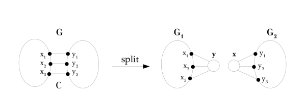
Figure 8: $C=\{(x_{1},y_{1}),(x_{2},y_{2}),(x_{3},y_{3})\}$ is a $3$-cut of $G$, with $\{x_{1},x_{2},x_{3}\}$ and $\{y_{1},y_{2},y_{3}\}$ lying in different connected components of $G\setminus{C}$. The split operation of $G$ at $C$ consists of the removal the edges of $C$ from $G$, and the introduction of two new nodes $x,y$, and six virtual edges $(x_{1},y),(x_{2},y),(x_{3},y),(x,y_{1}),(x,y_{2}),(x,y_{3})$. Now, the split graph is made of two connected components, $G_{1}$ and $G_{2}$. Every $3$-cut $C^{\prime}\neq C$ of $G$ (or more precisely: a $3$-cut that corresponds to $C^{\prime}$) lies entirely within $G_{1}$ or $G_{2}$. Conversely, every $3$-cut of either $G_{1}$ or $G_{2}$ corresponds to a $3$-cut of $G$. Thus, every $4$-edge-connected component of $G$ lies entirely within $G_{1}$ or $G_{2}$.

Now, due to the analysis of the preceding sections, we can distinguish the following types of $3$-cuts on a DFS-tree $T$ (see also Figure 1):

• (I) $\{(v,p(v)),(x_{1},y_{1}),(x_{2},y_{2})\}$, where $(x_{1},y_{1})$ and $(x_{2},y_{2})$ are back-edges.

• (IIa) $\{(u,p(u)),(v,p(v)),(x,y)\}$, where $u$ is a descendant of $v$ and $(x,y)\in B(v)$.

• (IIb) $\{(u,p(u)),(v,p(v)),(x,y)\}$, where $u$ is a descendant of $v$ and $(x,y)\in B(u)$.

• (III) $\{(u,p(u)),(v,p(v)),(w,p(w))\}$, where $w$ is an ancestor of both $u$ and $v$, but $u,v$ are not related as ancestor and descendant.

• (IV) $\{(u,p(u)),(v,p(v)),(w,p(w))\}$, where $u$ is a descendant of $v$ and $v$ is a descendant of $w$.

Let $r$ be the root of $T$. Then, for every $3$-cut $C\in\mathcal{C}$, $V_{C}$ is either $T(v)$, or $T(v)\setminus{T(u)}$, or $T(w)\setminus(T(u)\cup T(v))$, or $T(u)\cup(T(w)\setminus T(v))$, depending on whether $C$ is of type (I), (II), (III), or (IV), respectively. Thus we can immediately calculate the size of $C$ and the ends of its edges that lie in $V_{C}$. In particular, the size of $C$ is either $\mathit{ND}(v)$, or $\mathit{ND}(v)-\mathit{ND}(u)$, or $\mathit{ND}(w)-\mathit{ND}(u)-\mathit{ND}(v)$, or $\mathit{ND}(u)+\mathit{ND}(w)-\mathit{ND}(v)$, depending on whether it is of type (I), (II), (III), or (IV), respectively; $V_{C}$ contains either $\{v,x_{1},x_{2}\}$, or $\{p(u),v,x\}$, or $\{p(u),v,y\}$, or $\{p(u),p(v),w\}$, or $\{u,p(v),w\}$, depending on whether $C$ is of type (I), (IIa), (IIb), (III), or (IV), respectively.

Algorithm 12 shows how we can compute the $4$-edge-connected components of $G$ in linear time, by repeatedly splitting $G$ into smaller graphs according to its $3$-cuts. When we process a $3$-cut $C$ of $G$, we have to find the edges of the split graph that correspond to those of $C$, in order to delete them and replace them with (new) virtual edges. That is why we use the symbol $v^{\prime}$, for a vertex $v\in V$, to denote a vertex that corresponds to $v$ in the split graph. (Initially, we set $v^{\prime}\leftarrow v$.) Now, if $(x,y)$ is an edge of $C$ with $x\in V_{C}$, the edge of the split graph corresponding to $(x,y)$ is $(x^{\prime},y^{\prime})$. Then we add two new vertices $v_{C}$ and $\tilde{v_{C}}$ to $G$, and the virtual edges $(x^{\prime},\tilde{v_{C}})$ and $(v_{C},y^{\prime})$. Finally, we let $x$ correspond to $v_{C}$, and so we set $x^{\prime}\leftarrow v_{C}$. This is sufficient, since we process the $3$-cuts of $G$ in increasing order with respect to their size, and so the next time we meet the edge $(x,y)$ in a $3$-cut, we can be certain that it corresponds to $(v_{C},y^{\prime})$.

1 Find the collection $\mathcal{C}$ of the $3$-cuts of $G$

2 Locate and classify the $3$-cuts of $G$ on a DFS-tree of $G$ rooted at $r$

3 For every $C\in\mathcal{C}$, calculate $\mathit{size}(C)$ (relative to $r$)

4 Sort $\mathcal{C}$ in increasing order w.r.t. the $\mathit{size}$ of its elements

5 foreach $v\in V$ do Set $v^{\prime}\leftarrow v$

6 foreach $C=\{(x_{1},y_{1}),(x_{2},y_{2}),(x_{3},y_{3})\}\in\mathcal{C}$ do

       Find the ends of the edges of $C$ that lie in $V_{C}$ // Let those ends be $x_{1}$,$x_{2}$ and $x_{3}$

7       Remove the edges $(x_{1}^{\prime},y_{1}^{\prime})$,$(x_{2}^{\prime},y_{2}^{\prime})$,$(x_{3}^{\prime},y_{3}^{\prime})$ from $G$

8       Introduce two new vertices $v_{C}$ and $\tilde{v_{C}}$ to $G$

9       Add the edges $(x_{1}^{\prime},\tilde{v_{C}})$,$(x_{2}^{\prime},\tilde{v_{C}})$,$(x_{3}^{\prime},\tilde{v_{C}})$,$(v_{C},y_{1}^{\prime})$,$(v_{C},y_{2}^{\prime})$,$(v_{C},y_{3}^{\prime})$ to $G$

10       Set $x_{1}^{\prime}\leftarrow v_{C}$, $x_{2}^{\prime}\leftarrow v_{C}$, $x_{3}^{\prime}\leftarrow v_{C}$

11      

12 end foreach

13Output the connected components of $G$, ignoring the newly introduced vertices

Algorithm 12 Compute the $4$-edge-connected components of a $3$-edge-connected graph $G=(V,E)$

References

- [1] E. A. Dinitz, A. V. Karzanov, and M. V. Lomonosov. On the structure of a family of minimal weighted cuts in a graph. Studies in Discrete Optimization (in Russian), page 290–306, 1976.
- [2] Y. Dinitz. The 3-edge-components and a structural description of all 3-edge-cuts in a graph. In Proceedings of the 18th International Workshop on Graph-Theoretic Concepts in Computer Science, WG ’92, page 145–157, Berlin, Heidelberg, 1992. Springer-Verlag.
- [3] Y. Dinitz and J. Westbrook. Maintaining the classes of 4-edge-connectivity in a graph on-line. Algorithmica, 20:242–276, 1998. URL: https://doi.org/10.1007/PL00009195.
- [4] H. N. Gabow and R. E. Tarjan. A linear-time algorithm for a special case of disjoint set union. Journal of Computer and System Sciences, 30(2):209–21, 1985.
- [5] Z. Galil and G. F. Italiano. Reducing edge connectivity to vertex connectivity. SIGACT News, 22(1):57–61, March 1991. doi:10.1145/122413.122416.
- [6] L. Georgiadis and E. Kosinas. Linear-Time Algorithms for Computing Twinless Strong Articulation Points and Related Problems. In Yixin Cao, Siu-Wing Cheng, and Minming Li, editors, 31st International Symposium on Algorithms and Computation (ISAAC 2020), volume 181 of Leibniz International Proceedings in Informatics (LIPIcs), pages 38:1–38:16, Dagstuhl, Germany, 2020. Schloss Dagstuhl–Leibniz-Zentrum für Informatik. URL: https://drops.dagstuhl.de/opus/volltexte/2020/13382, doi:10.4230/LIPIcs.ISAAC.2020.38.
- [7] M. Ghaffari, K. Nowicki, and M. Thorup. Faster algorithms for edge connectivity via random 2-out contractions. In Proceedings of the Thirty-First Annual ACM-SIAM Symposium on Discrete Algorithms, SODA ’20, page 1260–1279, USA, 2020. Society for Industrial and Applied Mathematics.
- [8] M. Henzinger, S. Rao, and D. Wang. Local flow partitioning for faster edge connectivity. SIAM Journal on Computing, 49(1):1–36, 2020.
- [9] J. E. Hopcroft and R. E. Tarjan. Dividing a graph into triconnected components. SIAM Journal on Computing, 2(3):135–158, 1973.
- [10] A. Kanevsky and V. Ramachandran. Improved algorithms for graph four-connectivity. Journal of Computer and System Sciences, 42(3):288–306, 1991. URL: https://www.sciencedirect.com/science/article/pii/002200009190004O, doi:https://doi.org/10.1016/0022-0000(91)90004-O.
- [11] A. Kanevsky, R. Tamassia, G. Di Battista, and J. Chen. On-line maintenance of the four-connected components of a graph. In Proceedings 32nd Annual Symposium of Foundations of Computer Science (FOCS 1991), pages 793–801, 1991. doi:10.1109/SFCS.1991.185451.
- [12] D. R. Karger. Minimum cuts in near-linear time. Journal of the ACM, 47(1):46–76, January 2000. doi:10.1145/331605.331608.
- [13] D. R. Karger and D. Panigrahi. A near-linear time algorithm for constructing a cactus representation of minimum cuts. In Proceedings of the Twentieth Annual ACM-SIAM Symposium on Discrete Algorithms, SODA ’09, page 246–255, USA, 2009. Society for Industrial and Applied Mathematics.
- [14] K.-I. Kawarabayashi and M. Thorup. Deterministic edge connectivity in near-linear time. Journal of the ACM, 66(1), December 2018. doi:10.1145/3274663.
- [15] K. Menger. Zur allgemeinen kurventheorie. Fundamenta Mathematicae, 10(1):96–115, 1927.
- [16] H. Nagamochi and T. Ibaraki. A linear time algorithm for computing 3-edge-connected components in a multigraph. Japan J. Indust. Appl. Math, 9(163), 1992. doi:https://doi.org/10.1007/BF03167564.
- [17] H. Nagamochi and T. Ibaraki. Algorithmic Aspects of Graph Connectivity. Cambridge University Press, 2008. 1st edition.
- [18] H. Nagamochi and T. Watanabe. Computing -edge-connected components of a multigraph. IEICE Transactions on Fundamentals of Electronics, Communications and Computer Sciences, 76(4):513–517, 1993.
- [19] R. E. Tarjan. Depth-first search and linear graph algorithms. SIAM Journal on Computing, 1(2):146–160, 1972.
- [20] R. E. Tarjan. Finding dominators in directed graphs. SIAM Journal on Computing, 3(1):62–89, 1974.
- [21] R. E. Tarjan. Efficiency of a good but not linear set union algorithm. Journal of the ACM, 22(2):215–225, 1975.
- [22] Y. H. Tsin. Yet another optimal algorithm for 3-edge-connectivity. Journal of Discrete Algorithms, 7(1):130 – 146, 2009. Selected papers from the 1st International Workshop on Similarity Search and Applications (SISAP). URL: http://www.sciencedirect.com/science/article/pii/S1570866708000415, doi:https://doi.org/10.1016/j.jda.2008.04.003.