Supersymmetric black holes with spiky horizons

Abstract

We use the recipe of Klemm:2010mc to find half-BPS near-horizon geometries in the t³ model of $N=2$, $D=4$ gauged supergravity, and explicitely construct some new examples. Among these are black holes with noncompact horizons, but also with spherical horizons that have conical singularities (spikes) at one of the two poles. A particular family of them is extended to the full black hole geometry. Applying a double-Wick rotation to the near-horizon region, we obtain solutions with NUT charge that asymptote to curved domain walls with AdS₃ world volume. These new solutions may provide interesting testgrounds to address fundamental questions related to quantum gravity and holography.

1 Introduction and summary of results

Since the formulation of the AdS/CFT correspondence, asymptotically AdS black holes have been attracting much interest, partly due to their application to entropy calculations through the counting of black hole microstates (see Benini:2015eyy ; Benini:2016hjo ; Benini:2016rke for examples in $N=2$, $D=4$ Fayet–Iliopoulos (FI)-gauged supergravity). In this context gauged supergravity theories play an important role, since the gauging of (part of) the R-symmetry generically leads to a scalar potential which, in a vacuum configuration, behaves effectively as a cosmological constant and allows for non-asymptotically flat solutions that often (but not always) approach AdS at infinity.

It has been known for many years that a negative cosmological constant allows for black holes with non-spherical horizons, cf. e.g. Vanzo:1997gw and references therein. Gauged supergravity is thus an interesting terrain to study these kinds of black holes. Indeed, the scalar potential typically violates the assumptions that go into uniqueness theorems, so that one can have horizons that are flat, hyperbolic or compact Riemann surfaces of any genus Caldarelli:1998hg ; Cacciatori:2009iz ; DallAgata:2010ejj .

In these contexts, cubic models are of special interest. Like in the ungauged case, some cubic models in gauged supergravity can be embedded into higher-dimensional theories describing the low energy limit of some string theory. In particular, the FI-gauged stu model, containing three vector multiplets, can be obtained as a consistent truncation of eleven-dimensional supergravity compactified on a 7-sphere Duff:1999gh ; Cvetic:1999xp . A special subcase is the so-called t³ model, where the three vector multiplets are identified and which will be considered in this work.

Due to its importance, the gauged stu model has been extensively studied in the past. The first example appeared in Duff:1999gh , where the four-dimensional $N=2$ theory was obtained as a truncation of $N=8$ gauged supergravity, and static nonextremal black holes carrying electric or magnetic charges were presented. Subsequently, static and BPS generalizations were constructed in Cacciatori:2009iz ; Sabra:1999ux ; Chamseddine:2000bk ; Hristov:2010ri ; Katmadas:2014faa ; Halmagyi:2014qza , while nonextremal solutions to the t³ and stu models were found in Klemm:2012yg ; Klemm:2012vm . Rotation was added in Klemm:2011xw ; Gnecchi:2013mja , and more recently in Hristov:2018spe ; Daniele:2019rpr ; Hristov:2019mqp . Moreover, in Hristov:2018spe a general analysis of the possible asymptotic behaviours was performed by means of the real formulation of special geometry, in terms of a specific quartic form $I_{4}$ invariant under symplectic transformations. This provides a way to treat symplectically related prepotentials on the same footing, including theories which do not admit a prepotential. Although in the ungauged case all these theories lead to the same physics, the gauging breaks symplectic invariance, producing systems with different behaviours for the same gauge couplings, e.g. an AdS boundary at infinity or something completely different.

In this paper we will focus on the t³ model with prepotential $F=-(X^{1})^{3}/X^{0}$ and electric gauging. Using the classification of half-supersymmetric backgrounds presented in Klemm:2010mc , we will be able to obtain three classes of near-horizon solutions. Unfortunately, none of their possible full black hole extensions is expected to be asymptotically AdS₄ due to the absence of critical points of the scalar potential. Specifically, in section 2 we briefly review $N=2$, $D=4$ FI-gauged supergravity and the classifications of 1/4- and 1/2-BPS backgrounds given respectively in Cacciatori:2008ek and Klemm:2010mc . In section 3 we construct three new classes of near-horizon geometries, one of which turns out to be a generalization of the solution derived in section 4 of Daniele:2019rpr . Sections 4 and 5 are devoted to a deeper analysis of two of the new solutions, that can either have noncompact horizons, or spherical horizons with conical singularities (spikes) at one of the two poles. In 6 a full black hole extension of the third one is presented. Finally, applying a double-Wick rotation (which amounts to an analytical continuation of the coordinates) to the first two solutions, we obtain configurations with NUT charge that asymptote to curved domain walls with AdS₃ world volume, where AdS₃ appears as a Hopf-like fibration over H².

2 $N=2$, $D=4$ FI-gauged supergravity

2.1 The theory and BPS equations

We consider $N=2$, $D=4$ gauged supergravity coupled to $n$ abelian vector multiplets Andrianopoli:1996cm . Apart from the vierbein $e^{a}_{\mu}$, the bosonic field content includes the vectors $A^{I}_{\mu}$ enumerated by $I=0,\ldots,n$, and the complex scalars $z^{\alpha}$ where $\alpha=1,\ldots,n$. These scalars parametrize a special Kähler manifold, i.e., an $n$-dimensional Hodge–Kähler manifold that is the base of a symplectic bundle, with the covariantly holomorphic sections

$${\cal V}=\left(\begin{array}[]{c}X^{I}\\ F_{I}\end{array}\right)\,,\qquad{\cal D}_{\bar{\alpha}}{\cal V}=\partial_{\bar{\alpha}}{\cal V}-\frac{1}{2}(\partial_{\bar{\alpha}}{\cal K}){\cal V}=0\,,$$ (1)

where ${\cal K}$ is the Kähler potential and ${\cal D}$ denotes the Kähler-covariant derivative. ${\cal V}$ obeys the symplectic constraint

$$\langle{\cal V},\bar{\cal V}\rangle=X^{I}\bar{F}_{I}-F_{I}\bar{X}^{I}=i\,.$$ (2)

To solve this condition, one defines

$${\cal V}=e^{{\cal K}(z,\bar{z})/2}v(z)\,,$$ (3)

where $v(z)$ is a holomorphic symplectic vector,

$$v(z)=\left(\begin{array}[]{c}Z^{I}(z)\\ \frac{\partial}{\partial Z^{I}}F(Z)\end{array}\right)\,.$$ (4)

$F$ is a homogeneous function of degree two, called the prepotential, whose existence is assumed to obtain the last expression. The Kähler potential is then

$$e^{-{\cal K}(z,\bar{z})}=-i\langle v,\bar{v}\rangle\,.$$ (5)

The matrix ${\cal N}_{IJ}$ determining the coupling between the scalars $z^{\alpha}$ and the vectors $A^{I}_{\mu}$ is defined by the relations

$$F_{I}={\cal N}_{IJ}X^{J}\,,\qquad{\cal D}_{\bar{\alpha}}\bar{F}_{I}={\cal N}_{IJ}{\cal D}_{\bar{\alpha}}\bar{X}^{J}\,.$$ (6)

The bosonic action reads

$$\begin{split}e^{-1}{\cal L}_{\text{bos}}&=\frac{1}{2}R+\frac{1}{4}(\text{Im}\,{\cal N})_{IJ}F^{I}_{\mu\nu}F^{J\mu\nu}-\frac{1}{8}(\text{Re}\,{\cal N})_{IJ}\,e^{-1}\epsilon^{\mu\nu\rho\sigma}F^{I}_{\mu\nu}F^{J}_{\rho\sigma}\\ &\quad-g_{\alpha\bar{\beta}}\partial_{\mu}z^{\alpha}\partial^{\mu}\bar{z}^{\bar{\beta}}-V\,,\end{split}$$ (7)

with the scalar potential

$$V=-2g^{2}\xi_{I}\xi_{J}[(\text{Im}\,{\cal N})^{-1|IJ}+8\bar{X}^{I}X^{J}]\,,$$ (8)

that results from U$(1)$ Fayet–Iliopoulos gauging. Here, $g$ denotes the gauge coupling and the $\xi_{I}$ are FI constants. In what follows, we define $g_{I}\equiv g\xi_{I}$.

The most general timelike supersymmetric background of the theory described above was constructed in Cacciatori:2008ek , and is given by

$$ds^{2}=-4|b|^{2}(dt+\sigma)^{2}+|b|^{-2}(dz^{2}+e^{2\Phi}dwd\bar{w})\ ,$$ (9)

where the complex function $b(z,w,\bar{w})$, the real function $\Phi(z,w,\bar{w})$ and the one-form $\sigma=\sigma_{w}dw+\sigma_{\bar{w}}d\bar{w}$, together with the symplectic section (1) are determined by the equations

$$\partial_{z}\Phi=2ig_{I}\left(\frac{{\bar{X}}^{I}}{b}-\frac{X^{I}}{\bar{b}}\right)\ ,$$ (10)

$$\begin{split}&4\partial\bar{\partial}\left(\frac{X^{I}}{\bar{b}}-\frac{\bar{X}^{I}}{b}\right)+\partial_{z}\left[e^{2\Phi}\partial_{z}\left(\frac{X^{I}}{\bar{b}}-\frac{\bar{X}^{I}}{b}\right)\right]\\ &\qquad-2ig_{J}\partial_{z}\left\{e^{2\Phi}\left[|b|^{-2}(\text{Im}\,{\cal N})^{-1|IJ}+2\left(\frac{X^{I}}{\bar{b}}+\frac{\bar{X}^{I}}{b}\right)\left(\frac{X^{J}}{\bar{b}}+\frac{\bar{X}^{J}}{b}\right)\right]\right\}=0\,,\end{split}$$ (11)

$$\begin{split}&4\partial\bar{\partial}\left(\frac{F_{I}}{\bar{b}}-\frac{\bar{F}_{I}}{b}\right)+\partial_{z}\left[e^{2\Phi}\partial_{z}\left(\frac{F_{I}}{\bar{b}}-\frac{\bar{F}_{I}}{b}\right)\right]\\ &\qquad-2ig_{J}\partial_{z}\left\{e^{2\Phi}\left[|b|^{-2}\text{Re}\,{\cal N}_{IL}(\text{Im}\,{\cal N})^{-1|JL}+2\left(\frac{F_{I}}{\bar{b}}+\frac{\bar{F}_{I}}{b}\right)\left(\frac{X^{J}}{\bar{b}}+\frac{\bar{X}^{J}}{b}\right)\right]\right\}\\ &\qquad-8ig_{I}e^{2\Phi}\left[\langle{\cal I}\,,\partial_{z}{\cal I}\rangle-\frac{g_{J}}{|b|^{2}}\left(\frac{X^{J}}{\bar{b}}+\frac{\bar{X}^{J}}{b}\right)\right]=0\,,\end{split}$$ (12)

$$2\partial\bar{\partial}\Phi=e^{2\Phi}\left[ig_{I}\partial_{z}\left(\frac{X^{I}}{\bar{b}}-\frac{\bar{X}^{I}}{b}\right)+\frac{2}{|b|^{2}}g_{I}g_{J}(\text{Im}\,{\cal N})^{-1|IJ}+4\left(\frac{g_{I}X^{I}}{\bar{b}}+\frac{g_{I}\bar{X}^{I}}{b}\right)^{2}\right]\,,$$ (13)

$$d\sigma+2\,\star^{(3)}\!\langle{\cal I}\,,d{\cal I}\rangle-\frac{i}{|b|^{2}}g_{I}\left(\frac{\bar{X}^{I}}{b}+\frac{X^{I}}{\bar{b}}\right)e^{2\Phi}dw\wedge d\bar{w}=0\,.$$ (14)

Here $\star^{(3)}$ is the Hodge star on the three-dimensional base with metric

$$ds_{3}^{2}=dz^{2}+e^{2\Phi}dwd\bar{w}\,,$$ (15)

and we defined $\partial=\partial_{w}$, $\bar{\partial}=\partial_{\bar{w}}$, as well as

$${\cal I}=\text{Im}\left({\cal V}/\bar{b}\right)\,,\qquad{\cal R}=\text{Re}\left({\cal V}/\bar{b}\right)\,.$$ (16)

Note that the eqns. (10)-(13) can be written compactly in the symplectically covariant form

$$\partial_{z}\Phi=4\langle{\cal I},{\cal G}\rangle\,,$$ (17)

$$\begin{split}\Delta{\cal I}&+2e^{-2\Phi}\partial_{z}\left\{e^{2\Phi}\left[\langle{\cal R},{\cal I}\rangle\Omega{\cal M}{\cal G}-4{\cal R}\langle{\cal R},{\cal G}\rangle\right]\right\}\\ &-4{\cal G}\left[\langle{\cal I},\partial_{z}{\cal I}\rangle+4\langle{\cal R},{\cal I}\rangle\langle{\cal R},{\cal G}\rangle\right]=0\,,\end{split}$$ (18)

$$\Delta\Phi=-8\langle{\cal R},{\cal I}\rangle\left[{\cal G}^{t}{\cal M}{\cal G}+8|{\cal L}|^{2}\right]=4\langle{\cal R},{\cal I}\rangle V\,,$$ (19)

where ${\cal G}=(g^{I},g_{I})^{t}$ represents the symplectic vector of gauge couplings, ${\cal L}=\langle{\cal V},{\cal G}\rangle$, $\Delta$ denotes the covariant Laplacian associated to the base space metric (15), and $V$ in (19) is the scalar potential (8). Moreover,

$$\Omega=\left(\begin{array}[]{cc}0&1\\ -1&0\end{array}\right)\,,\qquad{\cal M}=\left(\begin{array}[]{cc}\text{Im}\,{\cal N}+\text{Re}\,{\cal N}(\text{Im}\,{\cal N})^{-1}\text{Re}\,{\cal N}&-\text{Re}\,{\cal N}(\text{Im}\,{\cal N})^{-1}\\ -(\text{Im}\,{\cal N})^{-1}\text{Re}\,{\cal N}&(\text{Im}\,{\cal N})^{-1}\end{array}\right)\,.$$ (20)

Finally, (14) can be rewritten as

$$d\sigma+\star_{h}\left(d\Sigma-A+\frac{1}{2}\nu\Sigma\right)=0\,,$$ (21)

where the function $\Sigma$ and the one-form $\nu$ are respectively given by

$$\Sigma=\frac{i}{2}\ln\frac{\bar{b}}{b}\,,\qquad\nu=\frac{8}{\Sigma}\langle{\cal G},{\cal R}\rangle dz\,,$$ (22)

$A$ is the gauge field of the Kähler U$(1)$,

$$A_{\mu}=-\frac{i}{2}(\partial_{\alpha}{\cal K}\partial_{\mu}z^{\alpha}-\partial_{\bar{\alpha}}{\cal K}\partial_{\mu}{\bar{z}}^{\bar{\alpha}})\,,$$ (23)

and $\star_{h}$ denotes the Hodge star on the Weyl-rescaled base space metric

$$h_{ij}dx^{i}dx^{j}=\frac{1}{|b|^{4}}(dz^{2}+e^{2\Phi}dwd\bar{w})\,.$$ (24)

(21) is the generalized monopole equation Jones:1985pla , or more precisely a Kähler-covariant generalization thereof, due to the presence of the one-form $A$. In order to cast (14) into the form (21), one has to use the special Kähler identities

$$\langle{\cal D}_{\alpha}{\cal V},{\cal V}\rangle=\langle{\cal D}_{\alpha}{\cal V},\bar{\cal V}\rangle=0\,.$$ (25)

Note that (21) is invariant under Weyl rescaling, accompanied by a gauge transformation of $\nu$,

$$h_{mn}{\rm d}x^{m}{\rm d}x^{n}\mapsto e^{2\psi}h_{mn}{\rm d}x^{m}{\rm d}x^{n}\,,\quad\Sigma\mapsto e^{-\psi}\Sigma\,,\quad\nu\mapsto\nu+2{\rm d}\psi\,,\quad A\mapsto e^{-\psi}A\,.$$ (26)

It would be very interesting to better understand the deeper origin of the conformal invariance of (21) in the present context.

The integrability condition for (21) reads

$$D_{i}[h^{ij}\sqrt{h}(D_{j}-A_{j})\Sigma]=0\,,$$ (27)

with the Weyl-covariant derivative

$$D_{i}=\partial_{i}-\frac{m}{2}\nu_{i}\,,$$ (28)

where $m$ denotes the Weyl weight of the corresponding field. It is straightforward to show that (27) is equivalent to

$$\langle{\cal I},\Delta{\cal I}\rangle+4e^{-2\Phi}\partial_{z}\left(e^{2\Phi}\langle{\cal I},{\cal R}\rangle\langle{\cal G},{\cal R}\rangle\right)=0\,,$$ (29)

which follows from (18) by taking the symplectic product with $\cal I$. To shew this, one has to use

$$\frac{1}{2}\left({\cal M}+i\Omega\right)=\Omega\bar{\cal V}{\cal V}\Omega+\Omega{\cal D}_{\alpha}{\cal V}g^{\alpha\bar{\beta}}{\cal D}_{\bar{\beta}}\bar{\cal V}\Omega,$$ (30)

$$\langle{\cal D}_{\alpha}{\cal V},{\cal D}_{\beta}{\cal V}\rangle=0\,,\qquad\langle{\cal D}_{\alpha}{\cal V},{\cal D}_{\bar{\beta}}\bar{\cal V}\rangle=-ig_{\alpha\bar{\beta}}\,,$$ (31)

as well as (17) and (25).

Given $b$, $\Phi$, $\sigma$ and $\cal V$, the fluxes read

$$\begin{split}F^{I}&=2(dt+\sigma)\wedge d\left[bX^{I}+\bar{b}\bar{X}^{I}\right]+|b|^{-2}dz\wedge d\bar{w}\left[\bar{X}^{I}(\bar{\partial}\bar{b}+iA_{\bar{w}}\bar{b})+({\cal D}_{\alpha}X^{I})b\bar{\partial}z^{\alpha}\right.\\ &\quad-\left.X^{I}(\bar{\partial}b-iA_{\bar{w}}b)-({\cal D}_{\bar{\alpha}}\bar{X}^{I})\bar{b}\bar{\partial}\bar{z}^{\bar{\alpha}}\right]-|b|^{-2}dz\wedge dw\left[\bar{X}^{I}(\partial\bar{b}+iA_{w}\bar{b})\right.\\ &\quad+\left.({\cal D}_{\alpha}X^{I})b\partial z^{\alpha}-X^{I}(\partial b-iA_{w}b)-({\cal D}_{\bar{\alpha}}\bar{X}^{I})\bar{b}\partial\bar{z}^{\bar{\alpha}}\right]\\ &\quad-\frac{1}{2}|b|^{-2}e^{2\Phi}dw\wedge d\bar{w}\left[\bar{X}^{I}(\partial_{z}\bar{b}+iA_{z}\bar{b})+({\cal D}_{\alpha}X^{I})b\partial_{z}z^{\alpha}-X^{I}(\partial_{z}b-iA_{z}b)\right.\\ &\quad-\left.({\cal D}_{\bar{\alpha}}\bar{X}^{I})\bar{b}\partial_{z}\bar{z}^{\bar{\alpha}}-2ig_{J}(\text{Im}\,{\cal N})^{-1|IJ}\right]\,.\end{split}$$ (32)

2.2 1/2-BPS near-horizon geometries

An interesting class of half-supersymmetric backgrounds was obtained in Klemm:2010mc . It includes the near-horizon geometry of extremal rotating black holes. The metric and the fluxes read respectively

$$ds^{2}=4e^{-\xi}\left(-r^{2}dt^{2}+\frac{dr^{2}}{r^{2}}\right)+4(e^{-\xi}-Ke^{\xi})(d\phi+r\,dt)^{2}+\frac{4e^{-2\xi}d\xi^{2}}{Y^{2}(e^{-\xi}-Ke^{\xi})}\,,$$ (33)

$$\begin{split}F^{I}&=16i\sqrt{K}\left(\frac{\bar{X}X^{I}}{1-iY}-\frac{X\bar{X}^{I}}{1+iY}\right)dt\wedge dr\\ &\quad+\frac{8\sqrt{K}}{Y}\left[\frac{2\bar{X}X^{I}}{1-iY}+\frac{2X\bar{X}^{I}}{1+iY}+\left(\mbox{Im}\,\mathcal{N}\right)^{-1|IJ}g_{J}\right](d\phi+r\,dt)\wedge d\xi\,,\end{split}$$ (34)

where $X\equiv g_{I}X^{I}$, $K>0$ is a real integration constant and $Y$ is defined by

$$Y^{2}=64e^{-\xi}|X|^{2}-1\,.$$ (35)

The moduli fields $z^{\alpha}$ depend on the horizon coordinate $\xi$ only, and obey the flow equation

$$\frac{dz^{\alpha}}{d\xi}=\frac{i}{2\bar{X}Y}(1-iY)g^{\alpha\bar{\beta}}{\cal D}_{\bar{\beta}}\bar{X}\ .$$ (36)

(33) is of the form (3.3) of Astefanesei:2006dd , and describes the near-horizon geometry of extremal rotating black holes, with isometry group $\text{SL}(2,\hbox{\mybb R})\times\text{U}(1)$. From (36) it is clear that the scalar fields have a nontrivial dependence on the horizon coordinate $\xi$ unless $g_{I}{\cal D}_{\alpha}X^{I}=0$. As was shown in Klemm:2010mc , the solution with constant scalars is the near-horizon limit of the supersymmetric rotating hyperbolic black holes in minimal gauged supergravity Caldarelli:1998hg .

Using $Y$ in place of $\xi$ as a new variable, (36) becomes

$$\frac{dz^{\alpha}}{dY}=\frac{Xg^{\alpha\bar{\beta}}{\cal D}_{\bar{\beta}}\bar{X}}{(Y-i)\left[-\bar{X}X+{\cal D}_{\gamma}Xg^{\gamma\bar{\delta}}{\cal D}_{\bar{\delta}}\bar{X}\right]}\,.$$ (37)

This can also be rewritten in a Kähler-covariant form, as a differential equation for the symplectic section $\cal V$,

$$D_{Y}{\cal V}=\frac{X{\cal D}_{\alpha}{\cal V}g^{\alpha\bar{\beta}}{\cal D}_{\bar{\beta}}\bar{X}}{(Y-i)\left[-\bar{X}X+{\cal D}_{\gamma}Xg^{\gamma\bar{\delta}}{\cal D}_{\bar{\delta}}\bar{X}\right]}\,,$$ (38)

where

$$D_{Y}\equiv\frac{d}{dY}+iA_{Y}$$ (39)

denotes the Kähler-covariant derivative.

2.3 The $\text{t}^{3}$ and square root model

The specific t³ model under investigation is defined by the prepotential

$$F=-\frac{{(X^{1})}^{3}}{X^{0}}\,.$$ (40)

As mentioned before, we work in a pure electric gauging, i.e. $\mathcal{G}=(0,0,g_{0},g_{1})^{t}$, and choose the parametrization

$$Z^{0}=1\,,\qquad Z^{1}=i\tau\,.$$ (41)

Then, the holomorphic symplectic vector, the Kähler potential, the scalar metric and the scalar potential are respectively given by

$$v=(1,i\tau,-i\tau^{3},3\tau^{2})^{t}\,,\qquad e^{-\mathcal{K}}=(\tau+\bar{\tau})^{3}\,,$$ (42)

and

$$g_{\tau\bar{\tau}}=\frac{3}{(\tau+\bar{\tau})^{2}}\,,\qquad V=-\frac{8g_{1}^{2}}{3(\tau+\bar{\tau})}\,.$$ (43)

Note that $V$ is of Liouville-type, and has thus no critical points, so the theory does not admit AdS₄ vacua with constant moduli.

A different model is defined by the prepotential

$$F=-2i(X^{0})^{1/2}(X^{1})^{3/2}\,.$$ (44)

If we take

$$Z^{0}=1\,,\qquad Z^{1}=\tau^{2}\,,$$ (45)

the holomorphic symplectic vector, Kähler potential and scalar metric become respectively

$$v=(1,\tau^{2},-i\tau^{3},-3i\tau)^{t}\,,\qquad e^{-\mathcal{K}}=(\tau+\bar{\tau})^{3}\,,\qquad g_{\tau\bar{\tau}}=\frac{3}{(\tau+\bar{\tau})^{2}}\,,$$ (46)

while the matrix $\cal N$ in (6) and the inverse of its imaginary part are given by

$${\cal N}=\frac{1}{3\tau-\bar{\tau}}\left(\begin{array}[]{cc}-2i\tau^{3}\bar{\tau}&3i\tau(\bar{\tau}-\tau)\\ 3i\tau(\bar{\tau}-\tau)&-6i\end{array}\right)\,,$$ (47)

$$(\text{Im}\,{\cal N})^{-1}=\frac{4}{3(\tau+\bar{\tau})^{3}}\left(\begin{array}[]{cc}-6&-\frac{3}{2}(\tau-\bar{\tau})^{2}\\ -\frac{3}{2}(\tau-\bar{\tau})^{2}&|\tau|^{2}(\tau^{2}-4\tau\bar{\tau}+{\bar{\tau}}^{2})\end{array}\right)\,.$$ (48)

Finally, the scalar potential reads

$$V=-\frac{8g_{1}}{3(\tau+\bar{\tau})}\left[3g_{0}+g_{1}|\tau|^{2}\right]\,,$$ (49)

which has a critical point at $\tau^{2}={\bar{\tau}}^{2}=3g_{0}/g_{1}$ that corresponds to an AdS vacuum.

3 Half-BPS rotating near-horizon geometries

3.1 t³ model

For the model defined by (40), the flow equation (37) boils down to

$$\frac{d\tau}{dY}=\frac{(\tau+\bar{\tau})\bigl{[}3\nu+i(\tau-2\bar{\tau})\bigr{]}(\nu+i\tau)}{6(Y-i)\bigl{(}-\nu^{2}-i\nu\tau+i\nu\bar{\tau}-\frac{1}{3}\tau\bar{\tau}+\frac{1}{3}\tau^{2}+\frac{1}{3}\bar{\tau}^{2}\bigr{)}},$$ (50)

where $\nu\equiv g_{0}/g_{1}$. It turns out that (50) can be solved using the assumption

$$\bar{\tau}=\tau-2i\mu\,,$$ (51)

with $\mu$ real and constant. This leads to

$$\frac{(-3\nu^{2}+6\nu\mu-4\mu^{2}-2i\mu\tau+\tau^{2})d\tau}{(\tau-i\mu)(\tau-i\nu)(\tau+3i\nu-4i\mu)}=\frac{dY}{Y-i}\,,$$ (52)

and thus

$$\tau=i\mu+(\mu-\nu)\Bigl{(}Y\pm\sqrt{Y^{2}-3}\Bigr{)}\,.$$ (53)

Note that a different class of half-BPS rotating near-horizon geometries in the $\text{t}^{3}$ model was obtained in Daniele:2019rpr . This is also of the form (33), but has $Y=-1/\sqrt{3}$ and is thus clearly not contained in the solutions derived above, where $Y$ was used as a coordinate.

A different way to deal with equation (50) is to define the shifted complex scalar

$$\hat{\tau}\equiv\tau-i\nu$$ (54)

and to split the flow equation in its real and imaginary parts,

$$\dfrac{d\hat{\tau}_{R}}{dY}=\hat{\tau}_{R}\dfrac{Y(\hat{\tau}_{R}^{2}+3\hat{\tau}_{C}^{2})+2\hat{\tau}_{R}\hat{\tau}_{C}}{(1+Y^{2})(\hat{\tau}_{R}^{2}-3\hat{\tau}_{C}^{2})}\,,\qquad\dfrac{d\hat{\tau}_{C}}{dY}=\hat{\tau}_{R}\dfrac{\hat{\tau}_{R}^{2}+3\hat{\tau}_{C}^{2}-2Y\hat{\tau}_{R}\hat{\tau}_{C}}{(1+Y^{2})(\hat{\tau}_{R}^{2}-3\hat{\tau}_{C}^{2})}\,,$$ (55)

where $\hat{\tau}_{R}\equiv\mathrm{Re}\hat{\tau}$ and $\hat{\tau}_{C}\equiv\mathrm{Im}\hat{\tau}$. We can easily decouple this system by defining the auxiliary function $f(Y)\equiv\hat{\tau}_{C}/\hat{\tau}_{R}$. In this way, we get

$$f^{\prime}=\frac{(1+f^{2})(1-3Yf)}{(1+Y^{2})(1-3f^{2})}\,.$$ (56)

A more convenient way of dealing with this equation is to suppose the function $f(Y)$ to be invertible and to rewrite (56) in terms of the inverse $Y(f)$,

$$Y^{\prime}=\frac{(1+Y^{2})(1-3f^{2})}{(1+f^{2})(1-3fY)}\,.$$ (57)

Since they will guide our steps in the construction of more solutions, we present here the expressions of $f(Y)$ and its inverse in the case of (53),

$$f(Y)=\frac{1}{Y\pm\sqrt{Y^{2}-3}}\,,\qquad Y(f)=\frac{1+3f^{2}}{2f}\,.$$ (58)

Inspired by these, we define $y(f)\equiv 2fY(f)$ and suppose a polynomial expansion for it. Then, it is straightforward to check that $y(f)$ can be at most of degree 2, and the only possible solutions are

$$Y(f)=\frac{1+3f^{2}}{2f}\,,\qquad Y(f)=\frac{1-f^{2}}{2f}\,,\qquad Y(f)=f\,,$$ (59)

with inverse

$$f(Y)=\frac{Y\pm\sqrt{Y^{2}-3}}{3}\,,\qquad f(Y)=-Y\pm\sqrt{Y^{2}+1}\,,\qquad f(Y)=Y\,.$$ (60)

The first solution is exactly (53), as expected. In order to find $\hat{\tau}_{R}$ and $\hat{\tau}_{C}$ in the remaining cases, the expression for $f$ has to be plugged into its definition to get $\hat{\tau}_{C}$ as a function of $\hat{\tau}_{R}$ (or viceversa), and with this relation one can try to solve the system (55). For the last two cases of (60), this leads respectively to

$$\tau=\mu\frac{\sqrt{Y^{2}+1}\mp 2Y}{\sqrt{Y^{2}+1}}\left(\pm Y+\sqrt{Y^{2}+1}\pm i\right)+i\nu\,,$$ (61)

$$\tau=\frac{\mu}{\sqrt{3Y^{2}-1}}\left(1+iY\right)+i\nu\,.$$ (62)

For the solution (62), the relation (35) between the coordinates $Y$ and $\xi$ boils down to

$$\mu=8g_{1}^{2}e^{-\xi}\sqrt{3Y^{2}-1}\,.$$ (63)

Plugging this into (62) gives

$$\tau=8g_{1}^{2}e^{-\xi}\left(1+iY\right)+i\nu\,,$$ (64)

which, contrary to (62), is well-defined also for $Y^{2}=1/3$. For $Y=-1/\sqrt{3}$ this corresponds exactly to the near-horizon solution costructed in Daniele:2019rpr , cf. (4.13) and (4.14) of Daniele:2019rpr . Eliminating $Y$ in (64) one gets

$$\tau=8g_{1}^{2}e^{-\xi}\left(1\pm\frac{i}{\sqrt{3}}\sqrt{1+e^{2\xi}\frac{\mu^{2}}{64g_{1}^{4}}}\right)+i\nu\,,$$ (65)

and thus the solution in Daniele:2019rpr is retrieved for $\mu=0$. It is worth noting that when the scalar is written in terms of $Y$, $\mu=0$ seems not to be an allowed value since, from the expression for the Kähler potential, $\mathrm{Re}\tau>0$. The origin of this discrepancy resides in the fact that (63) implies $Y=\pm 1/\sqrt{3}$ for $\mu=0$.

3.2 Square root model

For the model (44), we define a rescaled scalar field $z$ by

$$z=\left(\frac{g_{1}}{3g_{0}}\right)^{1/2}\tau\,,$$ (66)

such that the AdS critical point of the potential (49) is at $z=1$. Then the flow equation (37) becomes

$$\frac{dz}{dY}=\frac{\left(\frac{1}{3}+z^{2}\right)\left(-1-{\bar{z}}^{2}+2z\bar{z}\right)\left(z+\bar{z}\right)}{2(Y-i)\left[\frac{1}{3}-2z\bar{z}+z\bar{z}(z\bar{z}-z^{2}-{\bar{z}}^{2})\right]}\,.$$ (67)

Solutions for the square root prepotential are actually already known, since the model (44) with purely electric gauging is equivalent to the t³ model with mixed gauging considered in Hristov:2018spe . In fact, one can rotate the t³ model into (44) by a symplectic transformation with

$$\mathcal{S}=\begin{pmatrix}0&0&-\alpha^{-3}&0\\ 0&\alpha&0&0\\ \alpha^{3}&0&0&0\\ 0&0&0&\alpha^{-1}\\ \end{pmatrix}\,,$$ (68)

where $\alpha\in\mathbb{R}\!\setminus\!0$. Notice that $\mathcal{S}$ is fixed by the following constraints: First of all, it must be symplectic,

$$\mathcal{S}^{t}\Omega\mathcal{S}=\Omega\,,$$ (69)

with $\Omega$ given in (20). Moreover, the symplectic sections (1) must satisfy the constraint (2), and finally the prepotentials which describe the two models, (40) and (44), must be proportional, $F_{\text{sqrt}}\propto F_{\text{t}^{3}}$. It turns out that, in the present case, the correct relation is $F_{\text{sqrt}}=\pm 2F_{\text{t}^{3}}$. Without loss of generality we take the upper sign, which leads to (68).

The action of the symplectic rotation (68) on a generic vector of gauge couplings $\mathcal{G}=(g^{0},g^{1},g_{0},g_{1})^{t}$ is given by

$$\mathcal{G^{\prime}}=\mathcal{S}\mathcal{G}=\begin{pmatrix}-g_{0}/\alpha^{3}\\ g^{1}\alpha\\ g^{0}\alpha^{3}\\ g_{1}/\alpha\end{pmatrix},$$ (70)

and thus the mixed gauging of Hristov:2018spe ($g^{1}=g_{0}=0$) is rotated into the purely electric one considered here. Notice also that purely magnetic or purely electric gaugings are always rotated into mixed ones. Conversely, a mixed gauging may be rotated either into a pure or a mixed one, depending on which are the nonvanishing FI-parameters. For instance, $g^{0}=g_{1}=0$ is transformed into a purely magnetic gauging, while $g^{0}=g_{0}=0$ is rotated into a mixed one (with the same non-zero coupling constants).

Instead of $\mathcal{S}$, we can equally choose

$$\mathcal{S}^{\prime}=\begin{pmatrix}-\beta^{3}&0&0&0\\ 0&0&0&-\frac{1}{3\beta}\\ 0&0&-\frac{1}{\beta^{3}}&0\\ 0&3\beta&0&0\\ \end{pmatrix}$$ (71)

($\beta\in\mathbb{R}\!\setminus\!0$), which has the same effect, but leads to $F_{\text{sqrt}}=-2F_{\text{t}^{3}}$.

4 The first solution

In this section we construct the near-horizon black hole solution associated to the scalar (53). Introducing the new coordinate $p\equiv Y\pm\sqrt{Y^{2}-3}$ and shifting $\mu\to\mu+\nu$ for convenience, the scalar field takes the form

$$\tau=i(\mu+\nu)+\mu p\,,$$ (72)

while the metric is given by (33),

$$\begin{split}ds^{2}&=\frac{p(9+p^{2})\Delta}{8}\biggl{(}-r^{2}dt^{2}+\frac{dr^{2}}{r^{2}}\biggr{)}+\frac{p^{2}(9+p^{2})^{2}\Delta^{2}-1024K}{8p(9+p^{2})\Delta}(d\phi+rdt)^{2}\\ &\quad+\frac{9}{2}\frac{p^{3}(9+p^{2})\Delta^{3}}{p^{2}(9+p^{2})^{2}\Delta^{2}-1024K}dp^{2}\,,\end{split}$$ (73)

and the gauge potentials follow from (34),

$$A^{0} =-\frac{24g_{1}\sqrt{K}}{\mu^{2}p^{2}(9+p^{2})}(d\phi+rdt)\,,$$ (74a)

$$A^{1} =\frac{8g_{1}\sqrt{K}\left[3\nu+\mu(3+p^{2})\right]}{\mu^{2}p^{2}(9+p^{2})}(d\phi+rdt)\,,$$ (74b)

where we introduced the constant $\Delta\equiv\mu/g_{1}^{2}$.

In order to have the correct signature, we need $p\Delta>0$ and $p^{2}(9+p^{2})^{2}\Delta^{2}-1024K>0$. Without loss of generality we shall take $p>0$, $\Delta>0$, and thus $\mu>0$. Since $K$ and $p\Delta$ are both positive, the second constraint reduces to $f_{1}(p)\equiv p(9+p^{2})\Delta-32\sqrt{K}>0$. In our range of parameters the cubic polynomial $f_{1}$ is characterized by a negative discriminant and has therefore only one real root $\bar{p}$ which represents a coordinate singularity. Since the polynomial is positive for $p>\bar{p}$, our spacetime is defined in the interval $p\in(\bar{p},+\infty)$. Inspection of the scalar curvature shows the presence of a curvature singularity at $p=0$, which lies outside the allowed domain. The range of the periodic angular coordinate $\phi$ is fixed by imposing the absence of conical singularities. The induced metric on surfaces of constant $t,r$ can be written as

$$ds^{2}\bigl{|}_{t,r}=\frac{f_{1}(f_{1}+64\sqrt{K})}{8p(9+p^{2})\Delta}d\phi^{2}+\frac{9p^{3}(9+p^{2})\Delta^{3}}{2f_{1}(f_{1}+64\sqrt{K})}dp^{2}\,.$$ (75)

Close to the singularity $p\to\bar{p}$ this becomes

$$ds^{2}\bigl{|}_{t,r}\to\frac{3\bar{p}^{2}\Delta}{3+\bar{p}^{2}}\left[d\rho^{2}+\frac{(3+\bar{p}^{2})^{2}}{4\bar{p}^{2}}\rho^{2}d\phi^{2}\right]\,,$$ (76)

where $\rho^{2}\equiv p-\bar{p}$. A conical singularity in $p=\bar{p}$ ($\rho=0$) is thus avoided if we identify

$$\phi\sim\phi+\frac{4\pi\bar{p}}{3+\bar{p}^{2}}\,.$$ (77)

5 The second solution

Here we shall analyze the spacetime generated by the solution (61) to the flow equation. In doing this we follow the path traced in the previous section, to which we refer for further details.

We start defining $p\equiv Y\pm\sqrt{Y^{2}+1}$, which, for consistency, implies $p>0$ when the plus sign is taken and $p<0$ otherwise. Without loss of generality, in what follows we shall restrict to the first case. In terms of $p$ the scalar field becomes

$$\tau=\mu\frac{3-p^{2}}{1+p^{2}}(p+i)+i\nu\,,$$ (78)

the metric (33) reads

$$\begin{split}ds^{2}=\ &\frac{p(3-p^{2})\Delta}{8}\left(-r^{2}dt^{2}+\frac{dr^{2}}{r^{2}}\right)+\frac{p^{2}(3-p^{2})^{2}\Delta^{2}-1024K}{8p(3-p^{2})\Delta}(d\phi+rdt)^{2}\\ &+\frac{9}{2}\frac{p^{3}(3-p^{2})\Delta^{3}}{p^{2}(3-p^{2})^{2}\Delta^{2}-1024K}dp^{2}\,,\end{split}$$ (79)

and the gauge potentials are given by

$$A^{0} =\frac{8g_{1}\sqrt{K}}{\mu^{2}}\frac{1-3p^{2}}{p^{2}(3-p^{2})^{2}}(d\phi+rdt)\,,$$ (80a)

$$A^{1} =-\frac{8g_{1}\sqrt{K}}{\mu^{2}}\frac{\nu(1-3p^{2})+\mu(1-p^{2})(3-p^{2})}{p^{2}(3-p^{2})^{2}}(d\phi+rdt)\,,$$ (80b)

where, again, $\Delta\equiv\mu/g_{1}^{2}$.

The range of the coordinate $p$ is defined by $p(3-p^{2})\Delta>0$ and $p^{2}(3-p^{2})^{2}\Delta^{2}-1024K>0$, hence $f_{2}(p)\equiv p(3-p^{2})\Delta-32\sqrt{K}>0$. In this case the analysis of the polynomial $f_{2}$ is more complicated since the discriminant does not have a definite sign. For $\Delta<0$, $f_{2}$ has a local maximum at $p=p_{\text{M}}=-1$, where $f_{2}(p_{\text{M}})=-32\sqrt{K}+2|\Delta|$, and a local minimum at $p=p_{\text{m}}=1$, where $f_{2}(p_{\text{m}})=-32\sqrt{K}-2|\Delta|<0$. The polynomial $f_{2}$ has one root for $|\Delta|<16\sqrt{K}$, one single and one double root when the equality holds and three distinct zeroes for $|\Delta|>16\sqrt{K}$.

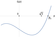
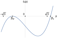
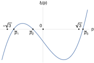
Figure 1: Graph of $f_{2}$ for: (a) $0>\Delta>-16\sqrt{K}$, (b) $\Delta=-16\sqrt{K}$, (c) $\Delta<-16\sqrt{K}$. Switching the sign of $\Delta$ produces a reflection of $f_{2}$ over the vertical axis.

From the possible graphs of $f_{2}$, shown in figure 1 for negative values of $\Delta$, we derive the following ranges of definition of $p$:

• $\Delta<0$: $p\in(\bar{p}_{3},+\infty)$ ,

• $0<\Delta\leq 16\sqrt{K}$: no interval ,

• $\Delta>16\sqrt{K}$: $p\in(\bar{p}_{2},\bar{p}_{1})$.

Notice that $\Delta$ determines the topology of the horizon, which is noncompact for $\Delta<0$ and compact for $\Delta>16\sqrt{K}$. Finally, the scalar curvature diverges in $p=0$ and $p=\pm\sqrt{3}$. Since $f_{2}(0)=f_{2}(\pm\sqrt{3})<0$, these points are located outside the allowed regions.

In order to fix the periodicity of the angular coordinate $\phi$ we restrict again to surfaces of constant $t$ and $r$. Close to a generic root $\bar{p}$ of $f_{2}$ the metric approaches

$$ds^{2}\bigl{|}_{t,r}\to\frac{3\bar{p}^{2}|\Delta|}{|1-\bar{p}^{2}|}\left[d\rho^{2}+\frac{(1-\bar{p}^{2})^{2}}{4\bar{p}^{2}}\rho^{2}d\phi^{2}\right]\,,$$ (81)

where again $\rho^{2}\equiv|p-\bar{p}|$. (81) is free from conical singularities in $p=\bar{p}$ if

$$\phi\sim\phi+\frac{4\pi\bar{p}}{|1-\bar{p}^{2}|}\,.$$ (82)

Let us now consider the case of a compact horizon, i.e., $\Delta>16\sqrt{K}$, $p\in(\bar{p}_{2},\bar{p}_{1})$. Since $\bar{p}_{2}$ lies at the left of the local maximum in $p=1$ and $\bar{p}_{1}$ on the right, we have $\bar{p}_{2}^{2}<1<\bar{p}_{1}^{2}$. Requiring the periodicities of $\phi$ in $\bar{p}_{1}$ and $\bar{p}_{2}$ to be equal gives thus

$$\frac{\bar{p}_{1}}{\bar{p}_{1}^{2}-1}=\frac{\bar{p}_{2}}{1-\bar{p}_{2}^{2}}\quad\Rightarrow\quad\bar{p}_{1}=\frac{1}{\bar{p}_{2}}\quad(\lor\,\bar{p}_{1}=-\bar{p}_{2})\,,$$ (83)

where the last case is excluded since we assumed $p>0$. We can then write

$$f_{2}(p)=p(3-p^{2})\Delta-32\sqrt{K}=-\Delta\left(p-\frac{1}{\bar{p}_{2}}\right)\!(p-\bar{p}_{2})(p-\bar{p}_{3})\,.$$ (84)

Comparing the coefficients of the various powers one obtains $\bar{p}_{2}=1$ and therefore also $\bar{p}_{1}=1$. One can thus remove only one of the two conical singularities located at the poles, and it is not possible to have a horizon that is smooth in both $\bar{p}_{1}$ and $\bar{p}_{2}$. The remaining singularity can be thought of as being created by a semi-infinite cosmological string. The horizon geometry is visualized by means of the embedding diagram in figure 2.

Figure 2: Embedding diagram of the horizon of the black hole (79) for $\Delta=86$ and $K=10$.

Alternatively, one can keep both singularities and tune the parameters of the metric such that the horizon becomes a specific kind of orbifold, the weighted projective space $\Sigma=\text{W}\mathbb{C}\text{P}^{1}_{[n_{1},n_{2}]}$, also called spindle (see Ferrero:2020laf ; Ferrero:2020twa ; Hosseini:2021fge for a list of recent references on this topic). This space is topologically a 2-sphere, but with conical singularities at the poles, characterized by deficit angles $2\pi(1-1/n_{1,2})$, with $n_{1,2}$ two coprime positive integers. Locally, the poles are modelled on $\mathbb{R}^{2}/\mathbb{Z}_{n_{1}}$ and $\mathbb{R}^{2}/\mathbb{Z}_{n_{2}}$. Fixing appropriately the constant $\sqrt{K}/\Delta$ and the period of $\phi$, the two-dimensional metric spanned by $p$ and $\phi$ becomes a smooth metric on the orbifold $\Sigma$.

5.1 Uplifting to $D=5$

Sometimes a better understanding of a given solution may be gained by taking advantage of the correlation between four and five-dimensional supergravity theories and studying the counterpart of the initial background. In this subsection we shall follow this strategy.

Let us consider the black hole solution (78)-(80) and uplift it to $N=2$, $D=5$ FI-gauged supergravity through the $r$-map (cf. appendix A). Since the starting point is the four-dimensional t³ model, the result will solve the equations of motion of five-dimensional pure gauged supergravity, whose bosonic sector consists of an Einstein-Maxwell theory with Chern-Simons term and cosmological constant. The oxidized solution reads

$$ds^{2} =\frac{1+x}{8g_{1}^{2}}\biggl{(}-r^{2}dt^{2}+\frac{dr^{2}}{r^{2}}\biggr{)}+\frac{1}{8g_{1}^{2}}\frac{(1+x)\bigl{[}x(3-x)^{2}-1024K\bigr{]}}{x(3-x)^{2}}(d\phi+rdt)^{2}$$ (85)

$$\quad\,+\frac{9}{8g_{1}^{1}}\frac{1+x}{x(3-x)^{2}-1024K}\,dx^{2}+\frac{x(3-x)^{2}}{(1+x)^{2}}\biggl{[}d\psi+\frac{8\sqrt{2K}}{g_{1}}\frac{1-3x}{x(3-x)^{2}}(d\phi+rdt)\biggr{]}^{2}\,,$$

$$A =\sqrt{3}\,\frac{3-x}{1+x}\,d\psi-\frac{8\sqrt{6K}}{g_{1}}\frac{1}{1+x}(d\phi+rdt)\,,$$

where we defined the new coordinate $x=p^{2}$ and rescaled $K\mapsto\Delta^{2}K$ in order to get rid of $\mu$.

Even though this expression may seem not very instructive, setting $K=0$ it is possible to retrieve the spindle solution of Ferrero:2020laf , namely equations (3)-(5), with $a=1$, a limiting case in which the horizon collapses to a circle. Despite the analogy between the four- and five-dimensional solutions, the two spindles have quite a different origin. Indeed, in the uplifted solution with vanishing $K$, $\phi$, which played the role of horizon coordinate in $D=4$, now parametrizes an AdS₃ space (cf. Ferrero:2020laf ), while the Kaluza–Klein coordinate $\psi$ gives birth, along with $x$, to the spindle.

6 Black hole extension

In what follows we shall construct and analyze the extension of the solution associated to (65) to the whole spacetime outside the black hole. To this end, it is convenient to rewrite the solution in a different coordinate system, which allows, by comparing to Daniele:2019rpr , to extend the metric to the region far from the horizon.

The metric is given by (33), where

$$Y(\xi)=\frac{1}{\sqrt{3}}\sqrt{1+\frac{\mu^{2}}{64g_{1}^{4}}e^{2\xi}}\,,$$ (86)

which follows from (63). The potentials related to the fluxes (34) are

$$A^{0} =-\frac{\sqrt{K}e^{2\xi}}{16g_{1}^{3}}(d\phi+rdt)\,,$$ (87a)

$$A^{1} =-\frac{\sqrt{K}e^{2\xi}}{16g_{1}^{3}}\left(\mp 8g_{1}^{2}e^{-\xi}Y(\xi)-\frac{g_{0}}{g_{1}}\right)(d\phi+rdt)\,.$$ (87b)

With the change of coordinates

$$e^{-\xi}=\sqrt{K}\coth\tilde{x}\,,\qquad\phi=\sqrt{3}y\,,\qquad t=\frac{T}{2\sqrt{K}}\,,$$ (88)

we can recast the scalar, metric and gauge potentials in a form that closely resembles the one in section 4.1 of Daniele:2019rpr ,

$$\tau=R(\tilde{x})\bigl{(}\sqrt{3}\pm iF(\tilde{x})\bigr{)}+i\frac{g_{0}}{g_{1}}\,,$$ (89)

$$ds^{2}=-\frac{8g_{1}^{2}}{\sqrt{3}R(\tilde{x})}\left(rdT+\frac{3}{4g_{1}^{2}}\partial_{\tilde{x}}R(\tilde{x})dy\right)^{2}+\frac{\sqrt{3}R(\tilde{x})}{2g_{1}^{2}}\left(\frac{dr^{2}}{r^{2}}+\frac{3(dx^{2}+dy^{2})}{\sinh^{2}\!\tilde{x}}\right),$$ (90)

$$A^{0} =-\frac{2g_{1}}{3R(\tilde{x})^{2}}\left(rdT+\frac{3}{4g_{1}^{2}}\partial_{\tilde{x}}R(\tilde{x})dy\right)\,,$$ (91a)

$$A^{1} =-\frac{2g_{1}}{3R(\tilde{x})^{2}}\left(\mp R(\tilde{x})F(\tilde{x})-\frac{g_{0}}{g_{1}}\right)\left(rdT+\frac{3}{4g_{1}^{2}}\partial_{\tilde{x}}R(\tilde{x})dy\right)\pm\frac{\coth\tilde{x}}{2g_{1}}F(\tilde{x})dy\,,$$ (91b)

where

$$R(\tilde{x})=\Xi_{1}\coth\tilde{x}\,,\qquad\Xi_{1}=8g_{1}^{2}\sqrt{\frac{K}{3}}\,,\qquad\frac{d\tilde{x}}{dx}=\mp F(\tilde{x})\equiv\mp\sqrt{1+\frac{\mu^{2}}{3R(\tilde{x})^{2}}}\,.$$ (92)

Inspired by Daniele:2019rpr , we make the following ansatz for the full black hole extension ($\alpha$ and $\beta$ are real constants):

$$\tau=\sqrt{3}\sqrt{\alpha r+\beta+R^{2}}\pm iRF+i\frac{g_{0}}{g_{1}}\,,$$ (93)

$$\begin{split}ds^{2}&=-\frac{8g_{1}^{2}}{\sqrt{3}\sqrt{\alpha r+\beta+R^{2}}}\left(rdT+\frac{3}{4g_{1}^{2}}\partial_{\tilde{x}}Rdy\right)^{2}\\ &\quad+\frac{\sqrt{3}\sqrt{\alpha r+\beta+R^{2}}}{2g_{1}^{2}}\left(\frac{dr^{2}}{r^{2}}+\frac{3(dx^{2}+dy^{2})}{\sinh^{2}\!\tilde{x}}\right),\end{split}$$ (94)

$$A^{0} =-\frac{2g_{1}}{3(\alpha r+\beta+R^{2})}\left(rdT+\frac{3}{4g_{1}^{2}}\partial_{\tilde{x}}Rdy\right),$$ (95a)

$$A^{1} =-\frac{2g_{1}}{3(\alpha r+\beta+R^{2})}\left(\mp RF-\frac{g_{0}}{g_{1}}\right)\left(rdT+\frac{3}{4g_{1}^{2}}\partial_{\tilde{x}}Rdy\right)\pm\frac{\coth\tilde{x}}{2g_{1}}Fdy\,,$$ (95b)

which we have shown to satisfy all the BPS equations of section 2.1. Eqns. (93)-(95) represent a generalization of the black hole solution constructed in section 4.1 of Daniele:2019rpr with $\Xi_{2}=0$. If the free parameter $\mu$ vanishes, our solution boils down to the one in Daniele:2019rpr with $\Xi_{2}=0$.

The spacetime (94) has a horizon for $r=0$, with induced metric

$$ds^{2}\bigl{|}_{t,r}=\frac{3\sqrt{3}}{2g_{1}^{2}\sinh^{2}\!\tilde{x}}\left[\sqrt{\beta+R^{2}}dx^{2}+\frac{\beta+\Xi_{1}^{2}}{\sqrt{\beta+R^{2}}}dy^{2}\right]\,.$$ (96)

As expected, the metric (94) is not asymptotically AdS₄ since the scalar potential in (43) has no critical points. A detailed physical discussion of the supersymmetric black hole given by (93)-(95) will be presented elsewhere.

6.1 Uplifting to $D=5$

In order to gain a deeper insight into this solution, once again we apply the $r$-map and uplift (93)-(95) to five dimensions. The five-dimensional background is

$$ds^{2} =-\frac{8g_{1}^{2}}{3f}\left(rdT+\frac{3}{4g_{1}^{2}}\partial_{\tilde{x}}Rdy\right)^{2}+\frac{1}{2g_{1}^{2}}\left(\frac{dr^{2}}{r^{2}}+\frac{3(dx^{2}+dy^{2})}{\sinh^{2}\!\tilde{x}}\right)$$ (97)

$$\quad\ +3f\left[dz-\frac{\sqrt{8}g_{1}}{3f}\left(rdT+\frac{3}{4g_{1}^{2}}\partial_{\tilde{x}}Rdy\right)\right]^{2}\,,$$

$$A =\pm F\coth\tilde{x}\left(\Xi_{1}dz+\frac{dy}{\sqrt{2}g_{1}}\right)\,,$$

where we defined

$$f(r,\tilde{x})=\alpha r+\beta+R(\tilde{x})^{2}\,.$$ (98)

Although written in an obscure form, this is actually a product space between an extremal BTZ black hole and the hyperbolic plane. To see this, start by shifting the $y$ coordinate as $\hat{y}=y+\sqrt{2}g_{1}\Xi_{1}z$, which yields a simplified expression for the metric and the gauge field,

$$ds^{2} =-\frac{8g_{1}^{2}}{3f_{0}}r^{2}dT^{2}+\frac{dr^{2}}{2g_{1}^{2}r^{2}}+\left(\sqrt{3f_{0}}dz-\frac{\sqrt{8}g_{1}}{\sqrt{3f_{0}}}rdT\right)^{2}+\frac{3}{2g_{1}^{2}}\frac{dx^{2}+d\hat{y}^{2}}{\sinh^{2}\!\tilde{x}}\,,$$ (99)

$$A =\pm\frac{F}{\sqrt{2}g_{1}}\coth\tilde{x}d\hat{y}\,,$$

with

$$f_{0}(r)=\alpha r+\beta+\Xi_{1}^{2}\,.$$ (100)

The canonical two-dimensional hyperbolic metric appears explicitely defining

$$\lambda\cosh\theta=\pm F\coth\tilde{x}\,,\qquad\phi=\hat{y}\sqrt{1+\frac{\mu^{2}}{3\Xi_{1}^{2}}}\,,$$ (101)

while the BTZ metric can be retrieved by the coordinate change

$$t=\frac{2g_{1}^{2}}{\sqrt{3}\alpha}T\,,\qquad\rho^{2}=f_{0}(r)\,,\qquad\psi=-\sqrt{\frac{3}{2}}g_{1}z+\frac{2g_{1}^{2}}{\sqrt{3}\alpha}T\,.$$ (102)

The result is

$$ds^{2} =\frac{2}{g_{1}^{2}}\left[-N^{2}dt^{2}+\frac{dr^{2}}{N^{2}}+\rho^{2}(d\psi+N^{\psi}dt)^{2}\right]+\frac{3}{2g_{1}^{2}}(d\theta^{2}+\sinh^{2}\!\theta d\phi^{2})\,,$$ (103)

$$A =\frac{1}{\sqrt{2}g_{1}}\cosh\theta d\phi\,,$$

where

$$N=\rho-\frac{\beta+\Xi_{1}^{2}}{\rho}\,,\qquad N^{\psi}=-\frac{\beta+\Xi_{1}^{2}}{\rho^{2}}\,,$$ (104)

which are, respectively, the lapse and shift functions that define an extremal BTZ black hole with mass $M=2(\beta+\Xi_{1}^{2})$. It is worth noting that the solution is described by the only free parameter $M$, contrary to the three constants characterizing the four-dimensional system. The behaviour we observe is somewhat unexpected: the full black hole solution (93)-(95) reduces to the near-horizon of a black string with momentum along the string once uplifted to five dimensions. Notice in this context that the extremal BTZ black hole preserves half of the supersymmetries of $(1,1)$ AdS supergravity in three dimensions Coussaert:1993jp and that the whole five-dimensional background can be proved to be 1/2-BPS, as expected for a near-horizon geometry.

7 Analytical continuation to NUT black holes

It is possible to analytically continue the near-horizon metric of an extremal rotating black hole to obtain a spacetime with NUT charge. In the following, we apply this procedure to a standard example, namely the extreme Kerr throat geometry, and then to the rotating near-horizon solutions described in the previous sections.

7.1 From the extremal Kerr black hole to a NUT spacetime

Let us consider the near-horizon metric of the extremal Kerr black hole Bardeen:1999px ,

$$ds^{2}=\frac{1+\cos^{2}\!\theta}{2}\biggl{(}-\frac{r^{2}}{r_{0}^{2}}dt^{2}+\frac{r_{0}^{2}}{r^{2}}dr^{2}+r_{0}^{2}d\theta^{2}\biggr{)}+\frac{2r_{0}^{2}\sin^{2}\!\theta}{1+\cos^{2}\!\theta}\biggl{(}d\phi+\frac{r}{r_{0}^{2}}dt\biggr{)}^{2}\,,$$ (105)

where the constant $r_{0}$ is related to the rotation parameter by $r_{0}^{2}=2a^{2}$.

We perform a double Wick rotation on the coordinates $t$ and $\phi$ by $t\to i\varphi$, $\phi\to i\tau$. Furthermore, we introduce the new radial coordinate $\rho=N\cos\theta$ and rename $a\to N$, where $N$ is interpreted as the NUT parameter. It is worth noting that after the analytic continuation the coordinate $r$ should not be considered radial anymore. Finally, the rescaling $r\to 2N^{2}r$ and $\tau\to\tau/2N$ brings the metric (105) to the form

$$ds^{2}=-f(\rho)(d\tau+2Nrd\varphi)^{2}+\frac{d\rho^{2}}{f(\rho)}+(N^{2}+\rho^{2})\biggl{(}r^{2}d\varphi^{2}+\frac{dr^{2}}{r^{2}}\biggr{)}\,,$$ (106)

where the radial function is defined as

$$f(\rho)=\frac{N^{2}-\rho^{2}}{N^{2}+\rho^{2}}\,.$$ (107)

Equation (106) is the hyperbolic NUT spacetime Taub:1950ez ; Newman:1963yy with parameter $N$.

7.2 NUT black holes

Since the supersymmetric near-horizon geometry (33) has the same form as (105), one can try to apply the analytical continuation outlined above also in that case. We shall do this for the two particular examples (73) and (79) to obtain black holes with NUT charge.

By Wick-rotating the coordinates $t\to i\varphi$, $\phi\to i\tau$ in (73), we find

$$\begin{split}ds^{2}&=-\frac{p^{2}(9+p^{2})^{2}\Delta^{2}-1024K}{8p(9+p^{2})\Delta}(d\tau+rd\varphi)^{2}\\ &\quad+\frac{9}{2}\frac{p^{3}(9+p^{2})\Delta^{3}}{p^{2}(9+p^{2})^{2}\Delta^{2}-1024K}dp^{2}+\frac{p(9+p^{2})\Delta}{8}\biggl{(}r^{2}d\varphi^{2}+\frac{dr^{2}}{r^{2}}\biggr{)}\,,\end{split}$$ (108)

where now $p$ has radial character. The very same transformations must be applied to the other fields of the theory, namely the fluxes and the scalar, and one can verify that the new fields still satisfy the equations of motion. Note also that (108) is of Petrov-type D. In order to have real gauge potentials and thus real charges, it is necessary to analytically continue the gauge coupling constant as well, $g\to-ig$. This implies $g_{I}\to-ig_{I}$, and thus (74) leads to

$$A^{0} =-\frac{24g_{1}\sqrt{K}}{\mu^{2}p^{2}(9+p^{2})}(d\tau+rd\varphi)\,,$$ (109a)

$$A^{1} =\frac{8g_{1}\sqrt{K}\left[3\nu+\mu(3+p^{2})\right]}{\mu^{2}p^{2}(9+p^{2})}(d\tau+rd\varphi)\,,$$ (109b)

while the scalar field is still given by (72). Note that the Wick rotation of the coupling constant amounts to changing the theory from genuine supergravity to fake supergravity Meessen:2009ma , where an $\mathbb{R}$-symmetry instead of a $\text{U}(1)$ is gauged. Introducing the new coordinate $R=p^{1/2}$ and taking the limit $R\to\infty$, the asymptotic metric takes the simple form of a domain wall,

$$ds^{2}=\frac{R^{6}}{144}\biggl{[}-(d\tau+rd\varphi)^{2}+r^{2}d\varphi^{2}+\frac{dr^{2}}{r^{2}}\biggr{]}+dR^{2}\,,$$ (110)

where we rescaled the metric by a factor of $18\Delta$. Notice that the world volume of this domain wall is curved, since the metric in brackets in (110) is AdS₃, written as a Hopf-like fibration over H², cf. e.g. Klemm:2014rda .

A second black hole with NUT charge can be generated by Wick-rotating the near-horizon geometry (79), which leads to

$$\begin{split}ds^{2}&=-\frac{p^{2}(3-p^{2})^{2}\Delta^{2}-1024K}{8p(3-p^{2})\Delta}(d\tau+rd\varphi)^{2}\\ &\quad+\frac{9}{2}\frac{p^{3}(3-p^{2})\Delta^{3}}{p^{2}(3-p^{2})^{2}\Delta^{2}-1024K}dp^{2}+\frac{p(3-p^{2})\Delta}{8}\left(r^{2}d\varphi^{2}+\frac{dr^{2}}{r^{2}}\right)\,,\end{split}$$ (111)

which is also of Petrov-type D, and $p$ is now a radial coordinate. Sending $g$ to $-ig$, the gauge potentials (80) become

$$A^{0} =\frac{8g_{1}\sqrt{K}(1-3p^{2})}{\mu^{2}p^{2}(3-p^{2})^{2}}(d\tau+rd\varphi)\,,$$ (112a)

$$A^{1} =-\frac{8g_{1}\sqrt{K}\left[\nu(1-3p^{2})+\mu(1-p^{2})(3-p^{2})\right]}{\mu^{2}p^{2}(3-p^{2})^{2}}(d\tau+rd\varphi)\,,$$ (112b)

and the scalar field is the same as in (78), with $\mu=g_{1}^{2}\Delta$. We have checked explicitely that (111), (112), together with (78), satisfy the equations of motion of fake gauged supergravity. For $\Delta<0$ and large $p$, the metric (111) asymptotes again to the domain wall (110), where $R=p^{1/2}$.

We conclude this section by noting that solutions (108) and (111) represent genuine black hole metrics. They both have a curvature singularity in $p=0$ covered by an event horizon. It is then appropriate to call them ‘NUT black holes’.

Appendix A $r$-map

$N=2$ gauged supergravity theories in four and five dimensions are closely related by a special dimensional reduction called $r$-map, which connects the latter to the subclass of four-dimensional theories with cubic prepotential

$$F=-\frac{1}{6}C_{\alpha\beta\gamma}\frac{X^{\alpha}X^{\beta}X^{\gamma}}{X^{0}}\,.$$ (113)

Here we shall consider vector multiplets only and focus on an abelian gauging, following the conventions of Klemm:2016kxw . The dimensional reduction is performed along an $S^{1}$ with compact coordinate $z$ by means of the Kaluza-Klein ansatz

$$\begin{gathered}ds_{(5)}^{2}=e^{\frac{\phi}{\sqrt{3}}}ds_{(4)}^{2}+e^{-\frac{2\phi}{\sqrt{3}}}(dz+K_{\mu}dx^{\mu})^{2}\,,\qquad A^{\alpha}=B^{\alpha}(dz+K_{\mu}dx^{\mu})+C^{\alpha}_{\mu}dx^{\mu}\,,\\ z^{\alpha}=e^{-\frac{\phi}{\sqrt{3}}}h^{\alpha}+iB^{\alpha}\,,\qquad e^{\mathcal{K}}=\frac{1}{8}e^{\sqrt{3}\phi}\,,\qquad F^{I}_{\mu\nu}=\frac{1}{\sqrt{2}}(dK_{\mu\nu},dC^{\alpha}_{\mu\nu})\,,\end{gathered}$$ (114)

where all the fields depend only on the four-dimensional coordinates $x^{\mu}$. We recall that $\alpha=1,\ldots,n$ and $I=0,\ldots,n$, and the complex scalars $z^{\alpha}$ are defined through the projection $z^{\alpha}=-iX^{\alpha}/X^{0}$. Moreover, one has to impose the constraints

$$g_{(4)}=3\sqrt{2}g_{(5)}\,,\qquad\xi_{0}=0\,,$$ (115)

where $g_{(4)}$ and $g_{(5)}$ are the gauge couplings in four and five dimensions respectively.

References

- (1) D. Klemm and E. Zorzan, “The timelike half-supersymmetric backgrounds of , supergravity with Fayet-Iliopoulos gauging”, Phys. Rev. D 82 (2010), 045012 [arXiv:1003.2974 [hep-th]].
- (2) F. Benini, K. Hristov and A. Zaffaroni, “Black hole microstates in from supersymmetric localization”, JHEP 05 (2016) 054 [arXiv:1511.04085 [hep-th]].
- (3) F. Benini and A. Zaffaroni, “Supersymmetric partition functions on Riemann surfaces”, Proc. Symp. Pure Math. 96 (2017) 13-46 [arXiv:1605.06120 [hep-th]].
- (4) F. Benini, K. Hristov and A. Zaffaroni, “Exact microstate counting for dyonic black holes in ”, Phys. Lett. B 771 (2017) 462-466 [arXiv:1608.07294 [hep-th]].
- (5) L. Vanzo, “Black holes with unusual topology”, Phys. Rev. D 56 (1997), 6475-6483 [arXiv:gr-qc/9705004 [gr-qc]].
- (6) M. M. Caldarelli and D. Klemm, “Supersymmetry of anti-de Sitter black holes”, Nucl. Phys. B 545 (1999), 434-460 [arXiv:hep-th/9808097 [hep-th]].
- (7) S. L. Cacciatori and D. Klemm, “Supersymmetric black holes and attractors”, JHEP 01 (2010), 085 [arXiv:0911.4926 [hep-th]].
- (8) G. Dall’Agata and A. Gnecchi, “Flow equations and attractors for black holes in U(1) gauged supergravity”, JHEP 03 (2011), 037 [arXiv:1012.3756 [hep-th]].
- (9) M. J. Duff and J. T. Liu, “Anti-de Sitter black holes in gauged supergravity”, Nucl. Phys. B 554 (1999), 237-253 [arXiv:hep-th/9901149 [hep-th]].
- (10) M. Cvetič et al., “Embedding AdS black holes in ten- and eleven dimensions”, Nucl. Phys. B 558 (1999), 96-126 [arXiv:hep-th/9903214 [hep-th]].
- (11) W. A. Sabra, “Anti-de Sitter BPS black holes in gauged supergravity,” Phys. Lett. B 458 (1999), 36-42 [arXiv:hep-th/9903143 [hep-th]].
- (12) A. H. Chamseddine and W. A. Sabra, “Magnetic and dyonic black holes in gauged supergravity,” Phys. Lett. B 485 (2000), 301-307 [arXiv:hep-th/0003213 [hep-th]].
- (13) K. Hristov and S. Vandoren, “Static supersymmetric black holes in AdS4 with spherical symmetry,” JHEP 04 (2011), 047 [arXiv:1012.4314 [hep-th]].
- (14) S. Katmadas, “Static BPS black holes in U(1) gauged supergravity”, JHEP 09 (2014), 027 [arXiv:1405.4901 [hep-th]].
- (15) N. Halmagyi, “Static BPS black holes in with general dyonic charges”, JHEP 03 (2015), 032 [arXiv:1408.2831 [hep-th]].
- (16) D. Klemm and O. Vaughan, “Nonextremal black holes in gauged supergravity and the real formulation of special geometry”, JHEP 01 (2013), 053 [arXiv:1207.2679 [hep-th]].
- (17) D. Klemm and O. Vaughan, “Nonextremal black holes in gauged supergravity and the real formulation of special geometry II”, Class. Quant. Grav. 30 (2013), 065003 [arXiv:1211.1618 [hep-th]].
- (18) D. Klemm, “Rotating BPS black holes in matter-coupled AdS4 supergravity”, JHEP 07 (2011), 019 [arXiv:1103.4699 [hep-th]].
- (19) A. Gnecchi, K. Hristov, D. Klemm, C. Toldo and O. Vaughan, “Rotating black holes in 4d gauged supergravity”, JHEP 01 (2014), 127 [arXiv:1311.1795 [hep-th]].
- (20) K. Hristov, S. Katmadas and C. Toldo, “Rotating attractors and BPS black holes in AdS4”, JHEP 01 (2019), 199 [arXiv:1811.00292 [hep-th]].
- (21) N. Daniele, F. Faedo, D. Klemm and P. F. Ramírez, “Rotating black holes in the FI-gauged , model”, JHEP 03 (2019), 151 [arXiv:1902.03113 [hep-th]].
- (22) K. Hristov, S. Katmadas and C. Toldo, “Matter-coupled supersymmetric Kerr-Newman-AdS4 black holes”, Phys. Rev. D 100 (2019) no.6, 066016 [arXiv:1907.05192 [hep-th]].
- (23) S. L. Cacciatori, D. Klemm, D. S. Mansi and E. Zorzan, “All timelike supersymmetric solutions of , gauged supergravity coupled to abelian vector multiplets”, JHEP 05 (2008), 097 [arXiv:0804.0009 [hep-th]].
- (24) L. Andrianopoli, M. Bertolini, A. Ceresole, R. D’Auria, S. Ferrara, P. Fré and T. Magri, “ supergravity and super-Yang-Mills theory on general scalar manifolds: Symplectic covariance, gaugings and the momentum map”, J. Geom. Phys. 23 (1997), 111-189 [arXiv:hep-th/9605032 [hep-th]].
- (25) D. Z. Freedman and A. Van Proeyen, “Supergravity”, Cambridge University Press (2012).
- (26) P. Jones and K. Tod, “Minitwistor spaces and Einstein-Weyl spaces”, Class. Quant. Grav. 2 (1985) no.4, 565.
- (27) D. Astefanesei, K. Goldstein, R. P. Jena, A. Sen and S. P. Trivedi, “Rotating attractors”, JHEP 10 (2006), 058 [arXiv:hep-th/0606244 [hep-th]].
- (28) J. M. Bardeen and G. T. Horowitz, “The Extreme Kerr throat geometry: A vacuum analog of ”, Phys. Rev. D 60 (1999), 104030 [arXiv:hep-th/9905099 [hep-th]].
- (29) P. Ferrero, J. P. Gauntlett, J. M. Pérez Ipiña, D. Martelli and J. Sparks, “D3-Branes Wrapped on a Spindle”, Phys. Rev. Lett. 126 (2021) no.11, 111601 [arXiv:2011.10579 [hep-th]].
- (30) P. Ferrero, J. P. Gauntlett, J. M. P. Ipiña, D. Martelli and J. Sparks, “Accelerating Black Holes and Spinning Spindles”, [arXiv:2012.08530 [hep-th]].
- (31) S. M. Hosseini, K. Hristov and A. Zaffaroni, “Rotating multi-charge spindles and their microstates”, [arXiv:2104.11249 [hep-th]].
- (32) O. Coussaert and M. Henneaux, “Supersymmetry of the (2+1) black holes”, Phys. Rev. Lett. 72 (1994), 183-186 [arXiv:hep-th/9310194 [hep-th]].
- (33) A. H. Taub, “Empty space-times admitting a three parameter group of motions”, Annals Math. 53 (1951) 472.
- (34) E. Newman, L. Tamburino and T. Unti, “Empty space generalization of the Schwarzschild metric”, J. Math. Phys. 4 (1963) 915.
- (35) P. Meessen and A. Palomo-Lozano, “Cosmological solutions from fake EYM supergravity”, JHEP 05 (2009), 042 [arXiv:0902.4814 [hep-th]].
- (36) D. Klemm, “Four-dimensional black holes with unusual horizons”, Phys. Rev. D 89 (2014) no.8, 084007 [arXiv:1401.3107 [hep-th]].
- (37) D. Klemm, N. Petri and M. Rabbiosi, “Black string first order flow in , abelian gauged supergravity”, JHEP 01 (2017), 106 [arXiv:1610.07367 [hep-th]].