Characterizing active learning environments in physics using latent profile analysis

Abstract

The vast majority of research involving active learning pedagogies uses passive lecture methods as a baseline. We propose to move beyond such comparisons to understand the mechanisms that make different active learning styles unique. Here, we use COPUS observations to record student and instructor activities in six known styles of active learning in physics, and use latent profile analysis to classify these observations. Latent profile analysis using two profiles successfully groups COPUS profiles into interactive lecture-like and other. Five latent profiles successfully sorts observations into interactive lecture-like, Modeling Instruction, ISLE labs, Context-Rich problems labs, and recitation/discussion-like. This analysis serves as a proof of concept, and suggests instructional differences across pedagogies that can be further investigated using this method.

I Introduction

Active learning has been gaining traction in physics classrooms, with numerous studies showing how active learning can promote learning gains over passive lecture alternatives. However, within the umbrella of ‘active learning’, several physics pedagogies have spawned from different ideological foundations, often with wildly varying mechanical differences Meltzer and Thornton (2012); Redish and Cooney (2007); Thacker (2003). As such, the term ‘active learning’ no longer sufficiently describes a pedagogy, making it difficult to pinpoint the mechanisms that lead to observed learning gains. Thus, it is imperative that we understand the mechanisms that make different ‘active learning in physics’ pedagogies unique, so future studies can further delineate the benefits of specific active learning mechanisms.

The ‘Characterizing active learning environments in physics’ project, or CALEP, sets out to establish a vocabulary that will allow us to speak about the different active learning pedagogies in physics, without relying on a comparison to passive lecture methods. We focused on two aspects of the active learning pedagogies, how students and instructors spend time in class, and the student networks that result from the instruction. A full summary of the CALEP project can be found in Commeford et al. (2020). We collected classroom observations and student network data from six prominent research-based introductory physics curricula. For the classroom observations, we used the Classroom Observation Protocol for Undergraduate STEM (COPUS)Smith et al. (2013), which allows us to measure the time dedicated to certain activities during a class-period, which, in essence, gives us an idea of the kinds of activities that occur in different active learning environments. For network analysis results, please refer to Commeford et al. (2020); Traxler et al. (2020).

This paper will focus on the COPUS observations, where we discuss the results of latent profile analysis (LPA) on the observed COPUS profiles. Latent profile analysis can be used to tease out hidden categories within your data– such as physics pedagogies. LPA has been used with COPUS data to describe a large sample of STEM classes, which effectively sorted them into active, passive, and hybrid categories Stains et al. (2018). Our analysis builds on that work by restricting to known active learning pedagogies in physics classrooms, as a first effort at developing a more nuanced classification scheme.

II Background

Because active learning is an umbrella term for different pedagogical approaches, it fails to identify distinguishing characteristics of pedagogies in physics. To this end, we identified six pedagogies that are well represented in the literature and at professional development workshops at national conferences. These six pedagogies have different approaches to active learning. In order to explore these different approaches, we used COPUS as a means to understanding unique features of classroom activity.

II.1 Active learning pedagogies in physics

We collected data from high fidelity implementations of six well known active learning pedagogies in physics. The pedagogies we studied were Tutorials in Introductory Physics, the Investigative Science Learning Environment (ISLE), Modeling Instruction, Peer Instruction, Context Rich Problems (aka the Minnesota curriculum), and SCALE-UP.

Tutorials in Introductory Physics maintains a lecture/lab/recitation structure typical of large introductory courses. The recitations, or tutorial sections, are interactive small group environments that have the students follow scaffolded worksheets that emphasize misconception confrontation and resolution. The teaching assistants facilitate small group interactions McDermott and Shaffer (2002); Scherr and Elby (2007).

ISLE (Investigative Science Learning Environment) treats students as neophyte scientists, and focuses on building up correct intuition rather than debunking misconceptions Etkina and Heuvelen (2007); Etkina (2015). Students work in small groups through a lab-based learning cycle, while the instructors facilitate discussion.

Modeling Instruction is a fully contained learning environment where students work in small groups to develop, test, deploy, and revise conceptual models, and then come together for large ‘white-board meetings’ to discuss their findings Phy ; Wells et al. (1995); Brewe (2008). The instructors facilitate small group discussion and guide the larger white-board meetings.

Peer Instruction is a structured, interactive lecture environment, typically used when classroom constraints deem a large lecture hall necessary. Peer Instruction divides a class session into small modules, which begin with a short lecture, and cycle through several clicker-questions. Students answer individually and then re-answer after discussing with their peers Mazur (1997); Crouch et al. (2007).

Context-rich problems leads students through the course under a pseudo apprentice-expert relationship. This pedagogy uses context-rich problems in all aspects of the course, to teach students how to identify relevant information and engage in expert-like problem solving behavior, as demonstrated by the instructor and teaching assistants Uni ; Heller and Hollabaugh (1992).

Finally, SCALE-UP is also a fully contained classroom environment, where the students are in pairs or groups of three, but seated at large tables with other groups of two or three students to facilitate larger discussions. SCALE-UP usually refers more to the classroom setup than the pedagogy itself, but lends itself nicely to the adoption of many active learning styles Beichner et al. (2007). As such, it is often treated as an independent pedagogy.

II.2 The Classroom Observation Protocol for Undergraduate STEM

The Classroom Observation Protocol for Undergraduate STEM (COPUS) was developed by Smith et.al Smith et al. (2013). It consists of 12 instructor and 13 student codes, for which the observer marks whether the coded behavior occurred or not during two-minute intervals. An activity is counted if the behavior occurs for at least five seconds during the two-minute interval. A full list of COPUS code abbreviations and their descriptions has been included in the supplementary material. An example of a COPUS observation for a tutorial session can be seen in table 1.

Table 1: COPUS observation example. Time is measured in two-minute intervals.

Students Doing

Instructor Doing

Time

L

IND

CG

WG

OG

AnQ

SQ

WC

Prd

SP

T/Q

W

O

Lec

RtW

Fup

PQ

CQ

AnQ

MG

1o1

D/V

Adm

W

O

0-2

X

X

X

X

X

2-4

X

X

X

X

X

4-6

X

X

X

X

X

6-8

X

X

X

X

8-10

X

X

X

X

10-12

X

X

X

X

12-14

X

X

14-16

X

X

X

X

16-18

X

X

X

X

18-20

X

X

X

Total

0

0

0

10

0

0

4

0

0

0

0

0

5

0

0

0

0

0

0

9

10

0

0

2

0

From these observations, we can compile the selected codes into COPUS profiles. The method of COPUS profile creation is not always clearly reported in literature that uses COPUS, making it difficult to compare analyses. It is typical of such studies to report percentages for each code, without a description of how ratios were taken or visualizations to infer the same information. As such, we explain our process here. For the CALEP project, we used the ‘bar chart’ method, in which COPUS profiles were created by summing the number of marks in each column (indicated in the ‘total’ row in table 1), and dividing by the number of intervals over which the observation occurred (10 intervals, using the same example). This method leads to the percentage of class time that a code was present. An example of a COPUS profile from CALEP can be seen in table 2. It should be noted, however, that we calculate our COPUS profiles differently than in Smith et.al. In Smith et.al., the number of marks is tallied for each column, and divided by the total number of marks across all columns. This method, which we dub ‘pie chart’ method, is useful when investigating the prevalence of activities. We chose the former method of profile creation, as we felt it provided a more explicit picture of how class time was spent. If an instructor spends the majority of the time lecturing, but peppers in several other instructional methods, the latter method of profile creation can be misleading and under-report the frequency of a code. We wanted a profile that showed the fraction of class time engaged in a certain instructional method, not fraction of every code reported.

Table 2: COPUS profile example. The total number of occurrences for each code was tallied in each column, and divided by the number of intervals. For this example, there were 10 intervals.

Students Doing		Instructor Doing
L	0	Lec	0
IND	0	RtW	0
CG	0	Fup	0
WG	1.0	PQ	0
OG	0	CQ	0
AnQ	0	AnQ	0
SQ	0.4	MG	0.9
WC	0	1o1	1.0
Prd	0	D/V	0
SP	0	Adm	0
T/Q	0	W	0.2
W	0	O	0
O	0.5

II.3 Latent Profile Analysis

Latent profile analysis (LPA) uses Gaussian mixture modeling to uncover hidden groupings, also known as classes or profiles, of data based on some measured variable Oberski (2016). For the CALEP project, our goal is to determine what the quantifiable identifying features of different physics pedagogies are. Active learning comes with an abundance of student-centered activities, which, in theory, are different for each pedagogy. As such, we chose to use LPA to see if this analysis method could identify different pedagogies based on observations of active learning behaviors. We used the percentage of class time per COPUS code (known as the COPUS profile) as our input variables to LPA, with the expectation that LPA would in turn group observations with similar COPUS profiles. Ideally, these groupings would align with the identified active learning pedagogies each observation represents.

II.4 Previous studies using LPA

Stains et. al. has previously utilized latent profile analysis with COPUS observations from several science disciplines Stains et al. (2018). They collected COPUS observations from classes across STEM disciplines, most of which were at doctoral-granting institutions, using a convenience approach– a call was put out on Discipline-Based Education Research (DBER) listservs asking researchers to share COPUS data, and they also collected voluntary COPUS submissions using the COPUS analyzer website Stains and Harshman . After using LPA on these solicited COPUS profiles, Stains ultimately chose the model with seven profiles for their data, which they further sorted into didactic (mostly lecture), interactive lecture (hybrid), or student centered (active) learning environments.

Stains et al took random observations and THEN classified them into active, passive, or hybrid pedagogies. We differ from Stains et al in that we used purposeful sampling, collecting data at sites chosen due to their high fidelity implementation of different active learning pedagogies. Further, we feel that it is no longer sufficient to be abstract in classifying pedagogies as ‘active’ or ‘not active’, so our purpose was to extend the work of Stains et al by zooming in on the active learning category, while limiting our scope to investigate differences among active learning specifically in physics.

We have provided a visual in figure 1 to help illustrate how LPA classifies COPUS profiles into distinct profiles. Given a distribution of an observed variable (in our case a single category from COPUS), shown in red, LPA assumes that this observed distribution can be described by a combination of distinct profiles that follow a Gaussian distribution (two groups, shown in blue and green). LPA begins by taking some initial Gaussian distribution to represent each profile, of which you can have any number, then iterates through the data and adjusts the Gaussians until all points are assigned to a profile such that the expectation value is maximized. LPA does this by calculating a probability distribution for each profile (the group Gaussians), and assigns a weighted profile membership to each data point (via probability distribution). It then recalculates the probability distribution representing each profile using the weighted members, and repeats this process until it converges.

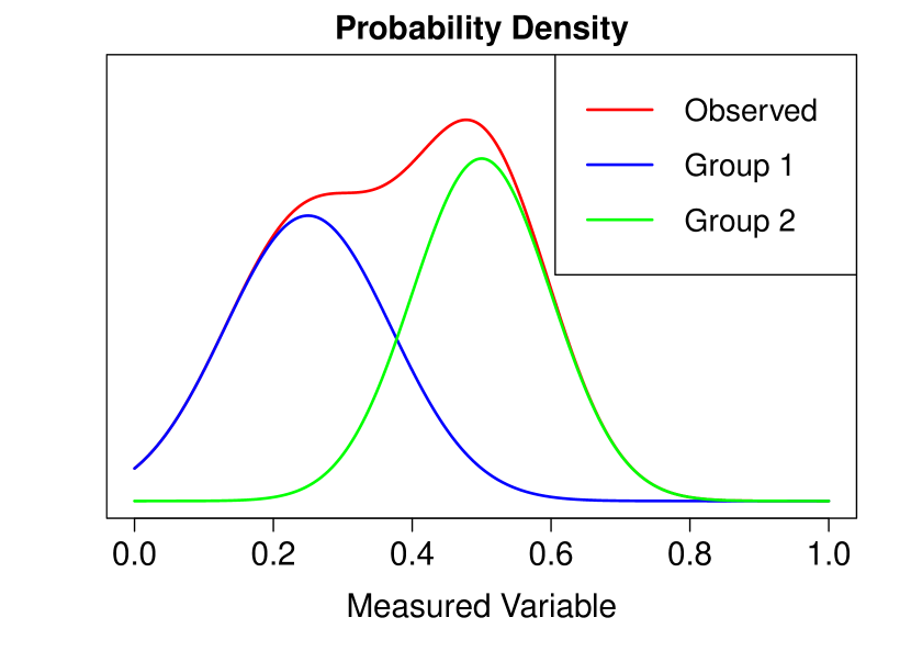
Figure 1: Given an observed distribution (red), LPA assumes that this observed distribution can be described by a combination of distinct profiles that follow a Gaussian distribution (two groups, shown in blue and green).

LPA can also accept constraints to these Gaussians, via variance and covariance. The variance can be equal between profiles (the Gaussians have the same width), or vary between profiles. Additionally, the prevalence of input variables can depend on each other, introducing co-variance, which can be set to zero, equal, or varying between profiles in the model as well Fraley and Raftery (2007). Understanding the variance of the profile distributions is a bit more straightforward if we preemptively reference the top panel of figure 2; The variance is the size of the box, and equal variance forces the size of the boxes for each code to be equal for each profile. Varying variance, on the other hand, allows these boxes to be different sizes. The co-variance describes how the input variables depend on each other, which is a bit harder to visualize. In the context of our data, co-variance would tell us how the presence of lecture depends on the presence of real-time-writing. While co-variance is likely present in our data (by observation, real-time-writing does typically accompany lecture), we did not have a large enough data set to get the varying co-variance model to converge. Additionally, the equal co-variance model, which forces each pedagogy to follow the same relationships between codes, was excluded as it was not an appropriate constraint for our study. Thus, we assume zero co-variance in our analysis. Future work should explore the role that co-variance plays in the development of profiles, where a larger data set can illuminate meaningful relationships between COPUS codes.

III Methods

We collected COPUS observations from six high fidelity active learning pedagogies in physics Commeford et al. (2020). We traveled to the sites and observed as many sections of the course as possible in a one week visitation period. All observations were done in a live environment, in person, by the same observer. The official COPUS recording spreadsheet was used for these data collections Smith et al. (2013). A summary of the number of sections and the number of observations per section can be seen in table 3.

Table 3: Number of course sections and observations for each pedagogy included in this study.

Pedagogy	Num. Sections	Num. Obs.
Tutorials	1 Lecture	1
	19 Tutorials	1
ISLE Whole Class	1 Lab	1
	4 Recitations	1
	1 Lecture	2
ISLE Lab Only	5 Labs	1
Modeling Instruction	3	2
Peer Instruction	1	1
Context-Rich Problems	2 Discussions	1
	4 Labs	1
	2 Lectures	2
SCALE-UP	1	3

From the base COPUS observations with checkmarks in each code column, we created the COPUS profiles by summing the number of checks per column and then dividing by the number of observation intervals (see section II.2 for a more thorough explanation of profile creation).

For this analysis, individual class period observations are left as stand-alone COPUS profiles. We originally wanted to cluster observations into a single profile to represent a week’s worth of class time for each pedagogy. This means, for example, an ISLE course that includes a lecture, recitation, and lab, would be reported as one COPUS profile that encapsulates the entire pedagogical experience for that week. Unfortunately, grouping observations in this way ensured we did not have enough data points for the LPA models to converge. As such, we left the COPUS profiles as individual class period observations, separated into various course components.

III.1 TidyLPA in R

There are six different LPA Gaussian mixture models that can be used in the TidyLPA package in R Rosenberg et al. (2018), two of which are run using wrappers to the proprietary software, Mplus Muthén and Muthén (1998). As such, those two models are not included in this analysis.

Each model specifies how the variance and co-variance of the Gaussian mixture models is altered between iterations. For equal variance, the variance of the fit Gaussians for each profile are assumed to be equal across profiles. The co-variance for inter-COPUS code relationships can be set to zero, equal between profiles, or varying between profiles. Table 4 illustrates the variance and co-variance combinations available, and their model number in TidyLPA.

Table 4: Variance and co-variance of TidyLPA model. Models 4 and 5 were not included, as they are run using the proprietary software, Mplus Muthén and Muthén (1998)

	Co-variance
Variance	Varying	Equal	Zero
Equal	MPLUS	3	1
Varying	6	MPLUS	2

In this paper, we show the results from model 1 analysis. Due to our relatively small data set, models 2 and 6 fail to converge. Model 3, which assumes equal co-variance between observed variables for each profile, was ultimately discarded as we felt it was not appropriate to force that condition. It would, however, be more interesting and realistic to use models 2 or 6, but we require more observations in order to get a convergent result.

IV Results

We ran LPA on our data using model 1 (equal variance between profiles, zero covariance) for 2-8 profiles. This range of profiles was originally chosen because it was the same range that is used in the TidyLPA vignette Rosenberg et al. (2018), but was ultimately kept after investigating the results. The sorting of observations into profiles becomes nonsensical after 8 profiles. We present the 2 profile and 5 profile solutions here, and include the remainder in supplemental material. The 2 profile solution is included due to the successful sorting of observations into ‘interactive lecture-like’ and ‘other’, as seen in Table 5. The top panel of figure 2 shows the box plots for each COPUS code and their associated profile groupings.

The five profile solution was included because it had the best BIC with the lowest number of profiles. This fit successfully sorted the COPUS observations into ‘interactive lecture-like’, Modeling Instruction, ISLE labs, CRP labs, and ‘recitation-like’ categories, as seen in Table 6. The lower panel of figure 2 shows the box plots for each COPUS code and their associated profile groupings.

Table 5: Model 1 profile assignment, 2 profiles. Profile 1 is red on the top panel of figure 2, while profile 2 is blue. ISLE had two sets of observations, the whole-class implementation (WC) and the lab-only implementation (LO).

Profile 1	Profile 2
Peer Instruction	ISLE LO Lab 1	Modeling 1.1	Tutorials 1	Tutorials 11
SCALE-UP 1.1	ISLE LO Lab 2	Modeling 1.2	Tutorials 2	Tutorials 12
SCALE-UP 1.2	ISLE LO Lab 3	Modeling 2.1	Tutorials 3	Tutorials 13
SCALE-UP 1.3	ISLE LO Lab 4	Modeling 2.2	Tutorials 4	Tutorials 14
ISLE WC Lecture 1.1	ISLE LO Lab 5	Modeling 3.1	Tutorials 5	Tutorials 15
ISLE WC Lecture 1.2	ISLE WC Lab 1	Modeling 3.2	Tutorials 6	Tutorials 16
CRP 1.1 Lecture	ISLE WC Recitation 1	CRP Discussion 1	Tutorials 7	Tutorials 17
CRP 1.2 Lecture	ISLE WC Recitation 2	CRP Discussion 2	Tutorials 8	Tutorials 18
CRP 2.1 Lecture	ISLE WC Recitation 3	CRP Lab 1	Tutorials 9	Tutorials 19
CRP 2.2 Lecture	ISLE WC Recitation 4	CRP Lab 2	Tutorials 10
Tutorials Lecture		CRP Lab 3
		CRP Lab 4

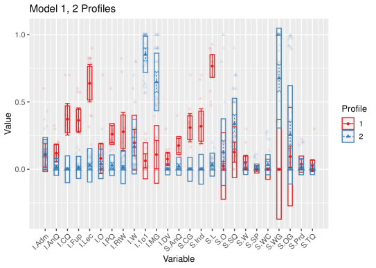
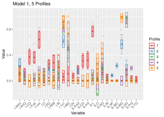
Figure 2: Model 1 shown for 2 profiles (top panel) and 5 profiles (bottom panel). The x-axis shows the full set of COPUS codes included in the analysis, while the y-axis shows the fraction of class time dedicated to that code. The light shaded dots show the actual COPUS profiles, colored by their assigned profile. The boxes show the standard deviation in each assigned profile, and the bars show the confidence interval of the centroid of said profile assignment. Since we used the equal variance model, the size of the boxes is equal between classes in each COPUS code.

Table 6: Model 1 profile assignment, 5 profile. Profile 1 is red in the lower panel in figure 2, profile 2 is blue, profile 3 is green, profile 4 is purple, and profile 5 is orange. ISLE had two sets of observations, the whole-class implementation (WC) and the lab-only implementation (LO).

Profile 1	Profile 2	Profile 3	Profile 4	Profile 5
Peer Instruction	Modeling 1.1	ISLE WC Lab 1	CRP Lab 1	ISLE WC Recitation 1
SCALE-UP 1.1	Modeling 1.2	ISLE LO Lab 1	CRP Lab 2	ISLE WC Recitation 2
SCALE-UP 1.2	Modeling 2.1	ISLE LO Lab 2	CRP Lab 3	ISLE WC Recitation 3
SCALE-UP 1.3	Modeling 2.2	ISLE LO Lab 3	CRP Lab 4	ISLE WC Recitation 4
ISLE WC Lecture 1.1	Modeling 3.1	ISLE LO Lab 4		CRP Discussion 1
ISLE WC Lecture 1.2	Modeling 3.2	ISLE LO Lab 5		CRP Discussion 2
CRP 1.1 Lecture				Tutorials 1
CRP 1.2 Lecture				Tutorials 2
CRP 2.1 Lecture				Tutorials 3
CRP 2.2 Lecture				Tutorials 4
Tutorials Lecture				Tutorials 5
				Tutorials 6
				Tutorials 7
				Tutorials 8
				Tutorials 9
				Tutorials 10
				Tutorials 11
				Tutorials 12
				Tutorials 13
				Tutorials 14
				Tutorials 15
				Tutorials 16
				Tutorials 17
				Tutorials 18
				Tutorials 19

The LPA algorithm uses hierarchical clustering to determine initial parameters, meaning the order of the data can have an effect on the resulting models. Stains et. al. combated this by shuffling their data and running the analysis 10,000 times. As this paper is proof of concept with a limited data set, we randomized the data five times to determine if further randomization was needed. After 5 additional analyses, there were zero discrepancies between profile assignments. As such, we did not run further randomization trials. The Bayesian information criterion (BIC) was used as the primary indicator of model acceptability. In general, the further left on the number line, the better the fit of the model. The BIC is plotted for model 1 against the number of profiles that the COPUS data was sorted into, which can be seen in figure 3. We see a slight increase in BIC from two to three profiles, and then a sharp drop until five profiles. Five, six, and seven profiles have nearly equal BIC values, before increasing again with eight profiles.

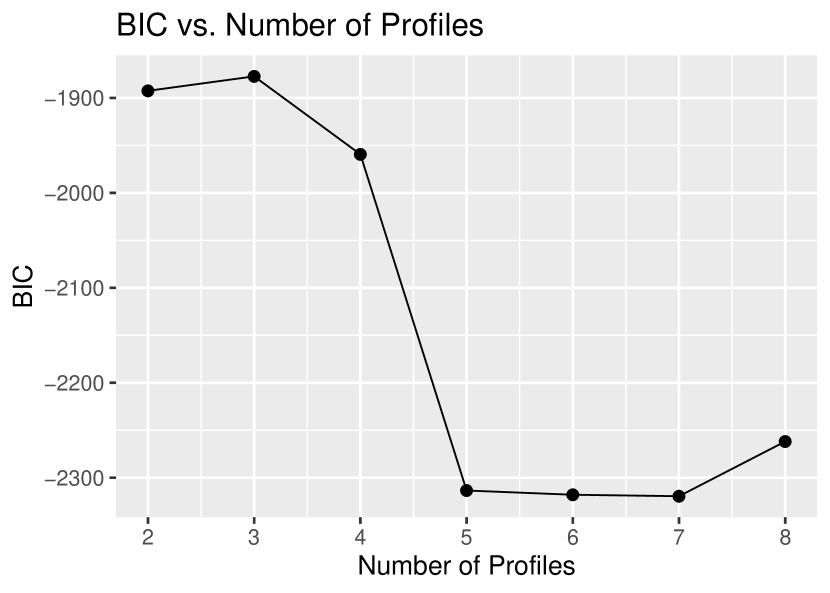
Figure 3: BIC vs number of profiles. We see a slight increase in BIC from two to three profiles, and then a sharp drop until five profiles. Five, six, and seven profiles have nearly equal BIC values, before increasing again with eight profiles. As such, we focus on two profiles and five profiles in further discussion.

V Discussion

V.1 Two Profiles

If we look more closely at the top panel of figure 2, we can start to pick apart the differences in the assigned profiles. The two profiles that emerged effectively sorted the observations into ‘large lecture-like’ and ‘other’. This becomes more apparent as we zoom into the individual codes. The largest separation between the two profiles occurs with the instructor lecturing (I.Lec), students listening (S.L), and the instructor having one on one conversations with students or small groups (I.1o1). If we think about how the observations were sorted (see table 5 for the full list), this makes sense. While Peer instruction and SCALE-UP are pedagogies that incorporate active learning techniques, they are still typically large classes where the bulk of information transfer occurs. Pair those with the lecture components of the other pedagogies, and we can see how I.Lec and S.L were the starkest differences from the profile that encompasses lab and recitation components. The lecture-like profile that we see in our data more closely aligns with the hybrid category (“active lecture”) that  Stains et al. (2018) reports.

The code where profile 2 takes the lead, I.1o1, indicates that instructors spend more time engrossed in individual discussions with students outside of large lecture-like environments. This is to be expected when comparing small, typically small-group activity-centered environments to a large information transfer environment. The outlier to this generalization is Modeling Instruction; a large enrollment course with very little information transfer from the instructor via lecture, and large amounts of small group learning activities (which is likely why it was grouped with recitation and lab components).

On the other hand, there were a few codes that were nearly indistinguishable between the two profiles, including administrative tasks (I.Adm), students and instructor waiting (S.W and I.W), test/quiz (S.TQ), students making a prediction (S.Prd), and student presentations (S.SP). The only pedagogy that had student presentations was Modeling Instruction, when the students gathered for their ‘white board meetings’. Only one observation had a test or quiz, given in the lecture component of Tutorials. Student prediction is for when students are explicitly asked to make a prediction about the outcome of a demo or experiment, which was also a very rare occurrence in our set of observations. Meanwhile, administrative tasks, waiting around for students to finish an activity or the instructor to begin the next part of the lesson, and other unclassifiable activities (like eating a snack or taking a restroom break), seem to be universal to all pedagogies.

Codes related to clicker questions or whole-class questioning were more common in the first profile, which is to be expected, as large enrollment courses are typically the environment for this instructional tool. These codes included I.CQ (instructor administers clicker question), I.Fup (instructor follows up a question with a longer discussion), I.PQ (instructor poses a non-rhetorical question to the whole class), S.AnQ (student answers a question with the whole class listening), S.CG (students work as a group to answer a clicker question), and S.Ind (students think independently to answer a question posed to the whole class).

While the first profile had very little group worksheet activity (S.WG) outside of SCALE-UP, the second profile had a large variance due to the wide array of group activities that are encompassed in these observations. Lab sections had mostly S.OG (other group activity), Tutorials had mostly S.WG, and Modeling Instruction had a mixture of both. As such, this code forced a large variance in the first profile as well, since we used model 1 during our latent profile analysis.

V.2 Five Profiles

Now let’s look more closely at the bottom panel of figure 2. Profile 1 (red boxes), which included lecture components and SCALE-UP observations, had a higher usage of clicker questions (I.CQ, S.CG, and S.Ind) and subsequent follow up (I.Fup). Profile 1 also had significantly higher usage of lecture (I.Lec) and thus students listening (S.L). Also noteworthy of profile 1 is a distinct lack of one-on-one discussions (I.1o1) and moving about the room to guide discussion (I.MG).

Profile 2 (blue boxes), which holds all of the Modeling Instruction observations, is the only pedagogy that used student presentations (S.SP) and whole class discussions (S.WC). Profile 2 also shows slightly less time engaged in one-on-one discussions than the other active profiles. Less time was also spent engaged in group worksheets (S.WG) than the other active profiles.

Profiles 3 and 4, which hold the ISLE labs and the Context Rich Problem labs, respectively, are a little more difficult to distinguish. The most notable difference between these two lab sortings is the use of student predictions (S.Prd) in the CRP labs. In these observations, students had to predict the outcome of their experiments and discuss as a group before jumping into the activity, whereas the ISLE labs were less explicitly structured in this regard. The CRP labs were actually the first group to separate from the two-profile solution due to this code (see 3 profiles in the supplementary material), followed by the ISLE labs in the 4 profile solution. It is also worth mentioning that the ISLE labs all go together, even though most are the stand-alone implementation and one is part of the full-class implementation. That suggests that the lab-only implementation had high fidelity to the goals of the whole-class ISLE implementation.

Finally, the recitation-like observations in profile 5 stand out with their abundance of group worksheet activities (S.WG). This profile also has elevated levels of moving around the room to guide discussion (I.MG), as well as students raising their hands to ask questions (S.SQ).

V.3 Further Discussion

Modeling Instruction and SCALE-UP are both studio format with a mingled lecture-lab-recitation, but were not binned in the same profiles for any number of profile fits. Unlike Modeling Instruction, the SCALE-UP class we observed still used lecture as the primary means of information transfer, whereas the bulk of information transfer in a Modeling environment is through exploration by the students and the subsequent whole class discussions. This, plus the usage of clicker questions, was the biggest difference between the seemingly similar studio-based pedagogies. As mentioned in the introduction of the pedagogies, SCALE-UP is more-so descriptive of the physical environment rather than specific activities, and lends itself well to a combination of many styles of active learning. It is therefore possible that the COPUS profile of a SCALE-UP course could vary wildly between implementations, but it is also possible that a unique SCALE-UP signature could emerge that encompasses all codes due to the physical capability to cover all codes. More observations from several institutions will be necessary to investigate further.

It is also interesting to see how all of the recitation/discussion observations were grouped in both 2 and 5 profile cases. The largest distinction between these and the lab sections was the usage of S.WG and S.OG. The bulk of recitation/discussion section activities was with small group worksheets, hence the WG ‘working in groups on a worksheet’ designation. Meanwhile, the labs were coded as ‘other group activity’, as COPUS does not include a code for this purpose. Without this distinction, there would likely be a lot of overlap between lab and recitation profile assignment, as the base behaviors of working in small groups while the instructor mills about the room were largely similar. For future work, we recommend exploring different observation protocols that can better capture the difference between group activities, or using both COPUS and LOPUS (Lab Observation Protocol for Undergraduate STEM, which is the lab variant of COPUS) Velasco et al. (2016).

VI Conclusion

We collected COPUS observations from six high-fidelity active learning pedagogies in physics. Using these observations, we performed latent profile analysis for 2-8 latent profile groupings. Two latent profiles successfully categorized the observations into ‘lecture-like’ and ‘not lecture-like’. Five latent profiles sorted the observations into ‘lecture-like’, Modeling Instruction, ISLE labs, Context-Rich labs, and recitation-like. With our preliminary data set, we made a first draft classification scheme using COPUS and LPA.

This was a proof of concept study, which showed great promise for using LPA to study how COPUS profiles can be used to classify physics active learning pedagogies. Stains et. al. suggest that at least four COPUS observations are required to get a good snapshot of the class, because day to day fluctuations had some instructors categorized into more than one cluster in their study. While we were unable to achieve this with our current iteration of data collection, we suggest future studies take this suggestion into account, and make a ‘combined COPUS profile’, consisting of several days worth of observations that include all components of a course (like lecure, lab, and recitation combined into one observation, as if a student were encountering the entire class). This method of data collection would allow us to more directly explore the difference between pedagogies, such as how a Peer Instruction experience with separate lab and recitation differs from a SCALE-UP integrated lab/lecture/recitation experience.

References

- Meltzer and Thornton (2012) D. E. Meltzer and R. K. Thornton, Am. J. Phys. 80, 478 (2012).
- Redish and Cooney (2007) E. F. Redish and P. J. Cooney, eds., Research-Based Reform of University Physics, Reviews in PER, Vol. 1 (American Association of Physics Teachers, 2007).
- Thacker (2003) B. A. Thacker, Reports on Progress in Physics 66, 1833 (2003).
- Commeford et al. (2020) K. Commeford, E. Brewe, and A. Traxler, Characterizing active learning environments in physics using network analysis and COPUS observations, Tech. Rep. (2020).
- Smith et al. (2013) M. K. Smith, F. H. M. Jones, S. L. Gilbert, and C. E. Wieman, CBE Life Sci. Educ. 12, 618 (2013).
- Traxler et al. (2020) A. L. Traxler, T. Suda, E. Brewe, and K. Commeford, Physical Review Physics Education Research 16, 020129 (2020).
- Stains et al. (2018) M. Stains, J. Harshman, M. K. Barker, S. V. Chasteen, R. Cole, S. E. DeChenne-Peters, M. K. Eagan, J. M. Esson, J. K. Knight, F. A. Laski, M. Levis-Fitzgerald, C. J. Lee, S. M. Lo, L. M. McDonnell, T. A. McKay, N. Michelotti, A. Musgrove, M. S. Palmer, K. M. Plank, T. M. Rodela, E. R. Sanders, N. G. Schimpf, P. M. Schulte, M. K. Smith, M. Stetzer, B. Van Valkenburgh, E. Vinson, L. K. Weir, P. J. Wendel, L. B. Wheeler, and A. M. Young, Science 359, 1468 (2018).
- McDermott and Shaffer (2002) L. C. McDermott and P. S. Shaffer, Tutorials in Introductory Physics, 1st ed. (Prentice Hall, Upper Saddle River, NJ, 2002).
- Scherr and Elby (2007) R. E. Scherr and A. Elby, AIP Conf. Proc. 883, 46 (2007).
- Etkina and Heuvelen (2007) E. Etkina and A. V. Heuvelen, in Reviews in PER: Research-Based Reform of University Physics, Vol. 1, edited by E. F. Redish and P. J. Cooney (American Association of Physics Teachers, College Park, MD, 2007).
- Etkina (2015) E. Etkina, Am. J. Phys. 83, 669 (2015).
- (12) “PhysPort Methods and Materials: University Modeling Instruction,” .
- Wells et al. (1995) M. Wells, D. Hestenes, and G. Swackhamer, Am. J. Phys. 63, 606 (1995).
- Brewe (2008) E. Brewe, Am. J. Phys. 76, 1155 (2008).
- Mazur (1997) E. Mazur, Peer Instruction: A User’s Manual, 1st ed. (Prentice Hall, Upper Saddle River, NJ, 1997).
- Crouch et al. (2007) C. Crouch, J. Watkins, A. Fagen, and E. Mazur, in Reviews in PER: Research-Based Reform of University Physics, Vol. 1, edited by E. F. Redish and P. J. Cooney (American Association of Physics Teachers, College Park, MD, 2007).
- (17) “University of Minnesota Physics Education Research and Development: Minnesota Model for Large Introductory Courses,” .
- Heller and Hollabaugh (1992) P. Heller and M. Hollabaugh, Am. J. Phys. 60, 637 (1992).
- Beichner et al. (2007) R. J. Beichner, J. M. Saul, D. S. Abbott, J. J. Morse, D. Deardorff, R. J. Allain, S. W. Bonham, M. H. Dancy, and J. S. Risley, in Reviews in PER: Research-Based Reform of University Physics, Vol. 1, edited by E. F. Redish and P. J. Cooney (American Association of Physics Teachers, College Park, MD, 2007).
- Oberski (2016) D. Oberski, in Modern statistical methods for HCI, edited by J. Robertson and M. Kaptein (Springer International Publishing, Switzerland, 2016) pp. 275–287.
- (21) M. Stains and J. Harshman, “COPUS Analyzer,” .
- Note (1) Victor Lavrenko does in incredible job illustrating how this process works on his YouTube channel http://bit.ly/EM-alg.
- Fraley and Raftery (2007) C. Fraley and A. E. Raftery, Journal of Classification 24, 155 (2007).
- Rosenberg et al. (2018) J. M. Rosenberg, P. N. Beymer, D. J. Anderson, C. J. Van Lissa, and J. A. Schmidt, Journal of Open Source Software 3, 978 (2018).
- Muthén and Muthén (1998) L. K. Muthén and B. O. Muthén, “Mplus User’s Guide,” (1998).
- Velasco et al. (2016) J. B. Velasco, A. Knedeisen, D. Xue, T. L. Vickrey, M. Abebe, and M. Stains, Journal of Chemical Education 93, 1191 (2016).