Practical and Rigorous Uncertainty Bounds for Gaussian Process Regression

Abstract

Gaussian Process Regression is a popular nonparametric regression method based on Bayesian principles that provides uncertainty estimates for its predictions. However, these estimates are of a Bayesian nature, whereas for some important applications, like learning-based control with safety guarantees, frequentist uncertainty bounds are required. Although such rigorous bounds are available for Gaussian Processes, they are too conservative to be useful in applications. This often leads practitioners to replacing these bounds by heuristics, thus breaking all theoretical guarantees. To address this problem, we introduce new uncertainty bounds that are rigorous, yet practically useful at the same time. In particular, the bounds can be explicitly evaluated and are much less conservative than state of the art results. Furthermore, we show that certain model misspecifications lead to only graceful degradation. We demonstrate these advantages and the usefulness of our results for learning-based control with numerical examples.

1 Introduction

Gaussian Processes Regression (GPR) is an established and successful nonparametric regression method based on Bayesian principles (Rasmussen and Williams 2006) which has recently become popular in learning-based control (Liu et al. 2018; Kocijan 2016). In this context, safety and performance guarantees are important aspects (Åström and Murray 2010; Skogestad and Postlethwaite 2007). In fact, the lack of rigorous guarantees has been identified as one of the major obstacles preventing the usage of learning-based control methodologies in safety-critical areas like autonomous driving, human-robot interaction or medical devices, see e.g. (Berkenkamp 2019). One approach to tackle this challenge is to use the posterior variance of GPR to derive frequentist uncertainty bounds and combine these with robust control methods that can deal with the remaining uncertainty. This strategy has been successfully applied in a number of works that also provide control-theoretical guarantees, cf. Section 2.2.

These approaches rely on rigorous frequentist uncertainty bounds for GPR. Although such results are available (Srinivas et al. 2010, Theorem 6), (Chowdhury and Gopalan 2017, Theorem 2), they turn out to be very conservative and difficult to evaluate numerically in practice and are, hence, replaced by heuristics. That is, instead of bounds obtained from theory, much smaller ones are assumed, sometimes without any practical justification, cf. Section 2.3 for more discussion. Unfortunately, using heuristic approximations leads to a breakdown of the theoretical guarantees of these control approaches, as already observed for example in (Lederer, Umlauft, and Hirche 2019). Furthermore, when deriving theoretical guarantees based on frequentist results like (Srinivas et al. 2010, Theorem 6) or (Chowdhury and Gopalan 2017, Theorem 2), model misspecifications (like wrong hyperparameters of the underlying GPR model or approximations such as the usage of sparse GPs) are ignored. Since model misspecifications are to be expected in any realistic setting, the validity of such theoretical guarantees based on idealized assumptions is unclear.

In summary, rigorous and practical frequentist uncertainty bounds for GPR are currently not available. By practical we mean that concrete, not excessively conservative numerical bounds can be computed based on reasonable and established assumptions and that these are robust against model misspecifications at least to some extent. We note that such bounds are of independent interest, for example, for Bayesian Optimization (Shahriari et al. 2015). In this work, we improve previous frequentist uncertainty bounds for GPR leading to practical, yet theoretically sound results. In particular, our bounds can be directly used in algorithms and are sharp enough to avoid the use of unjustified heuristics. Furthermore, we provide robustness results that can handle moderate model misspecifications. Numerical experiments support our theoretical findings and illustrate the practical use of the bounds.

2 Background

2.1 Gaussian Process Regression and Reproducing Kernel Hilbert Spaces

We briefly recall the basics of GPR, for more details we refer to (Rasmussen and Williams 2006). A Gaussian Process (GP) over an (input or index) set $D$ is a collection of random variables, such that any finite subset is normally distributed. A GP $f$ is uniquely determined by its mean function $m(x)=\mathbb{E}[f(x)]$ and covariance function $k(x,x^{\prime})=\mathbb{E}[(f(x)-m(x))(f(x^{\prime})-m(x^{\prime}))]$ and we write $f\sim\mathcal{G}_{D}(m,k)$. Without loss of generality we focus on the case $m\equiv 0$. Common covariance functions include the Squared Exponential (SE) and Matern kernel. Consider a Gaussian Process prior $f\sim\mathcal{G}_{D}(0,k)$ and noisy data $(x_{i},y_{i})_{i=1,\ldots,N}$, where $x_{i}\in D$ and $y_{i}=f(x_{i})+\epsilon_{i}$ with i.i.d. $\mathcal{N}(0,\sigma^{2})$ noise, then the posterior is also a GP, with the posterior mean $\mu_{N}$, posterior covariance $k_{N}$ and posterior variance given by

$$\mu_{N}(x) =\mu(x)+\boldsymbol{k}_{N}(x)^{T}(\boldsymbol{K}_{N}+\sigma^{2}\mathcal{I}_{N})^{-1}\boldsymbol{y}_{N}$$

$$k_{N}(x,x^{\prime}) =k(x,x^{\prime})-\boldsymbol{k}_{N}(x)^{T}(\boldsymbol{K}_{N}+\sigma^{2}\mathcal{I}_{N})^{-1}\boldsymbol{k}_{N}(x^{\prime})$$

$$\sigma_{N}^{2}(x) =k_{N}(x,x),$$

where we defined the kernel matrix $\boldsymbol{K}_{N}=(k(x_{j},x_{i}))_{i,j=1,\ldots,N}$ and the column vectors $\boldsymbol{k}_{N}(x)=(k(x_{i},x))_{i=1,\ldots,N}$ and $\boldsymbol{y}_{N}=(y_{i})_{i=1,\ldots,N}$.

Later on we follow (Srinivas et al. 2010; Chowdhury and Gopalan 2017) and assume that the ground truth is a function from a Reproducing Kernel Hilbert Space (RKHS). For an introduction to the RKHS framework we refer to (Steinwart and Christmann 2008, Chapter 4) or (Berlinet and Thomas-Agnan 2011) as well as (Kanagawa et al. 2018) for connections between Gaussian Processes and the RKHS framework.

2.2 Bayesian and Frequentist Bounds

GPR is based on Bayesian principles: A prior distribution is chosen (here a GP with given mean and covariance function) and then updated with the available data using Bayes rule, assuming a certain likelihood or noise model (here independent Gaussian noise). The updated distribution is called the posterior distribution and can be interpreted as a tradeoff between prior belief (encoded in the prior distribution together with the likelihood model) and evidence (the data) (Murphy 2012, Chapter 5). In contrast to the Bayesian approach, in frequentist statistics the existence of a ground truth is assumed and noisy data about this ground truth is acquired (Murphy 2012, Chapter 6).

For many applications which require safety guarantees it is important to get reliable frequentist uncertainty bounds. A concrete setting and major motivation for this work is learning-based robust control. Here, the ground truth is an only partially known dynamical system and the goal is to solve a certain control task, like stabilization or tracking, by finding a suitable controller. A machine learning method like GPR is used to learn more about the unknown dynamical system from data. Thereafter a set of possible models is derived from the learning method that contains the ground truth with a given (high) probability. For this reason such a set is often called an uncertainty set. We then use a robust method on this set, i.e., a method the leads to a controller that works for every element of this set. Since the ground truth is contained in this set with a given (high) probability, the task is solved with this (high) probability. Examples of such an approach are (Koller et al. 2018) (using robust model predictive control with state constraints), (Umlauft et al. 2017) (using feedback linearization to achieve ultimate boundedness) and (Helwa, Heins, and Schoellig 2019) (considering tracking of Lagrangian systems).

The control performance typically degrades with larger uncertainty sets, and it might even be impossible to achieve the control goal if the uncertainty sets are too large (Skogestad and Postlethwaite 2007). Therefore it is desirable to extract uncertainty sets that are as small as possible, but still include the ground truth with a given high probability. In particular, when using GPR, this necessitates frequentist uncertainty bounds that are not too conservative, so that the uncertainty sets are not too large. Furthermore, we also have to be able to evaluate the uncertainty bounds numerically, since robust control methods typically need an explicit uncertainty set.

For learning-based control applications using GPR together with robust control methods, bounds of the following form have been identified as the most useful ones: Let $X$ be an arbitrary input set and assume that $f:X\rightarrow\mathbb{R}$ is the unknown ground truth. Let $\mu_{N}$ be the posterior mean using a dataset of size $N$, generated from the ground truth, and let $\delta\in(0,1)$ be given. We need a function $\nu_{N}(x)$ that can be explicitly evaluated, such that with probability at least $1-\delta$ with respect to the data generating process, we have

$$|f(x)-\mu_{N}(x)|\leq\nu_{N}(x)\>\forall x\in X.$$ (1)

We emphasize that the probability statement is with respect to the noise generating process, and that the underlying ground truth is just some deterministic function. For a more thorough discussion we refer to (Berkenkamp 2019, Section 2.5.3).

2.3 Related Work

Frequentist uncertainty bounds for GPR as considered in this work were originally developed in the literature on bandits. To the best of our knowledge, the first result in this direction was (Srinivas et al. 2010, Theorem 6), which is of the form (1) with $\nu_{N}(x)=\beta_{N}\sigma_{N}(x)$. Here $\beta_{N}$ is a constant that depends on the maximum information gain, an information theoretic quantity. For common settings, there exist upper bounds on the latter quantity, though these increase with sample size. The result from (Srinivas et al. 2010) has been significantly improved in (Chowdhury and Gopalan 2017, Theorem 2), though the latter still uses an upper bound depending on the maximum information gain. The importance of (Srinivas et al. 2010, Theorem 6) and (Chowdhury and Gopalan 2017, Theorem 2) for other applications outside the bandit setting has been recognized early on, in particular in the control community, for example in (Berkenkamp, Schoellig, and Krause 2016; Berkenkamp et al. 2016; Koller et al. 2018; Berkenkamp 2019; Umlauft et al. 2017; Helwa, Heins, and Schoellig 2019).

Unfortunately, both (Srinivas et al. 2010, Theorem 6) and (Chowdhury and Gopalan 2017, Theorem 2) tend to be very conservative, especially for control applications (Berkenkamp, Schoellig, and Krause 2016; Berkenkamp 2019). Furthermore, both results rely on an upper bound of the maximum information gain, which can be difficult to evaluate (Srinivas et al. 2010), though asymptotic bounds are available for standard kernels like the linear, SE or Matern kernel. However, for most control applications, these asymptotic bounds are not useful since one requires a concrete numerical bound in the nonasymptotic setting.

For these reasons, previous work utilizing (Srinivas et al. 2010, Theorem 6) or (Chowdhury and Gopalan 2017, Theorem 2) used heuristics. In the control community, it is common to choose a constant value $\beta_{N}\equiv\beta$ in an ad-hoc manner, see for example (Berkenkamp et al. 2017, 2016; Koller et al. 2018; Berkenkamp, Schoellig, and Krause 2016; Helwa, Heins, and Schoellig 2019). This choice does not reflect the asymptotic behaviour of the scaling since the maximum information gain grows with the number of samples (Srinivas et al. 2010). The problem with such heuristics is that they might work in practice, but all theoretical guarantees that are based on results like (Chowdhury and Gopalan 2017, Theorem 2) are lost, in particular, safety guarantees like constraint satisfaction or certain stability notions. This is especially problematic since one of the major incentives to use GPR together with such results is to provably ensure properties like stability of a closed loop system.

Note that in concrete applications one has to make some assumptions on the ground truth at some point. However, it is not clear at all how a constant scaling $\beta$ as used in these heuristics can be derived from real-world properties in a principled manner. In contrast to such heuristics, in the original bounds (Srinivas et al. 2010, Theorem 6), (Chowdhury and Gopalan 2017, Theorem 2) every ingredient (i.e., desired probability, size of noise, bound on RKHS norm) has a clear interpretation.

It seems to be well-known in the multiarm-bandit literature that, in the present situation, it is possible to use more empirical bounds than (Chowdhury and Gopalan 2017, Theorem 2). Such approaches are conceptually similar to the results that we will present in Section 3 below, cf. (Abbasi-Yadkori 2013) and the recent work (Calandriello et al. 2019). However, to the best of our knowledge, results like Theorem 1 are rarely used in applications. In particular, it seems that no attempts have been made in the control community to use such a-posteriori bounds in the GPR context.

Model misspecification in the context of GPR has been discussed before in some works. In (Beckers, Umlauft, and Hirche 2018) a numerical method for bounding the mean-squared-error of a misspecified GP is considered, but it relies on a probabilistic setting. The recent article (Wang, Tuo, and Jeff Wu 2019) provides uniform error bounds and deals with misspecified kernels, but again uses a probabilistic setting and focuses on the noise-free case.

A work with goals similar to ours is (Lederer, Umlauft, and Hirche 2019). The authors recognize and explicitly discuss some of the problems of (Chowdhury and Gopalan 2017, Theorem 2) in the context of control. However, (Lederer, Umlauft, and Hirche 2019) uses a probabilistic setting, while our work is concerned with a fixed, but unknown underlying target function, and hence our results are of a worst-case nature. As we argued in Section 2.2, this is the setting required for robust approaches. Finally, the very recent work (Maddalena, Scharnhorst, and Jones 2020) requires bounded noise and does not deal with model misspecification.

3 Practical and Rigorous Frequentist Uncertainty Bounds

We now present our main technical contributions. The key observation is that for many applications relying on frequentist uncertainty bounds, in particular, learning-based control methods, only a-posteriori bounds are needed. This means that the frequentist uncertainty set can be derived after the learning process and hence the concrete realization of the dataset can be used. We take advantage of this fact and modify existing uncertainty results so that they explicitly depend on the dataset used for learning. In general no a-priori guarantees can be derived from the results we present here, but this does not play a role in the present setting.

The following result, which is a modified version of (Chowdhury and Gopalan 2017, Theorem 2), is fundamental for the rest of the paper.

Theorem 1.

Let $D\not=\emptyset$ be a set and $k:D\times D\rightarrow\mathbb{R}$ a positive definite kernel with corresponding RKHS $~{}{(H_{k},\|\cdot\|_{k})}$ and let $f\in H_{k}$ with $\|f\|_{k}\leq B$ for some $B\geq 0$. Let $\mathbb{F}=(\mathcal{F}_{n})_{n\in\mathbb{N}}$ be a filtration and $(x_{n})_{n\in\mathbb{N}}$ a $D$-valued discrete-time stochastic process that is predictable w.r.t. $\mathbb{F}$ and let $(\epsilon_{n})_{n}$ be an $\mathbb{R}$-valued stochastic process adapted to $\mathbb{F}$, such that $\epsilon_{n}$ conditioned on $\mathcal{F}_{n-1}$ is $R$-subgaussian with $R\geq 0$. Furthermore, define $y_{n}=f(x_{n})+\epsilon_{n}$ for all $n\geq 1$.

Consider a Gaussian process $g\sim\mathcal{G}_{D}(0,k)$ and denote its posterior mean function by $\mu_{N}$, its posterior covariance function by $k_{N}$ and its posterior variance by $\sigma^{2}_{N}(x):=k_{N}(x,x)$, w.r.t. to data $(x_{1},y_{1}),\ldots,(x_{N},y_{N})$, assuming in the likelihood independent Gaussian noise with mean zero and variance $\lambda>0$. Then for any $\delta\in(0,1)$ with $\bar{\lambda}=\max\{1,\lambda\}$ and

$$\beta_{n} =\beta_{n}(\delta,B,R,\lambda)$$

$$=B+\frac{R}{\sqrt{\lambda}}\sqrt{\log\left(\operatorname{det}(\bar{\lambda}/\lambda\boldsymbol{K}_{n}+\bar{\lambda}\mathcal{I}_{n})\right)-2\log(\delta)}$$ (2)

one has

$$\mathbb{P}\left[|\mu_{N}(x)-f(x)|\leq\beta_{N}\sigma_{N}(x)\>\forall N\in\mathbb{N},x\in D\right]\geq 1-\delta.$$ (3)

Proof.

(Idea) Essentially identical to the proof of (Chowdhury and Gopalan 2017, Theorem 2), however, we do not upper-bound (1) by the maximum information gain. Details are given in the supplementary material. ∎

The key insight is that by appropriate modifications of the proof of (Chowdhury and Gopalan 2017, Theorem 2) we obtain a frequentist uncertainty bound for GPR that fulfills all desiderata from Section 2.2. In the numerical examples below we show that the bound is often tight enough for practical purposes.

Independent inputs and noise (e.g. deterministic inputs and i.i.d. noise) is a common situation that is simpler than the setting of Theorem 1. In this case the following a-posteriori bound can be derived that does not depend anymore on $\log\operatorname{det}$.

Proposition 2.

Let $D\not=\emptyset$ be a set and $k:D\times D\rightarrow\mathbb{R}$ a positive definite kernel with corresponding RKHS $(H_{k},\|\cdot\|_{k})$ and let $f\in H_{k}$ with $\|f\|_{k}\leq B$ for some $B\geq 0$. Let $x_{1},\ldots,x_{N}\in D$ be given and $\epsilon_{1},\ldots,\epsilon_{N}$ be $\mathbb{R}$-valued independent $R$-subgaussian random variables. Furthermore, define $y_{n}=f(x_{n})+\epsilon_{n}$ for all $n=1,\ldots,N$.

Consider a Gaussian process $g\sim\mathcal{G}_{D}(0,k)$ and denote its posterior mean function by $\mu_{N}$, its posterior covariance function by $k_{N}$ and its posterior variance by $\sigma^{2}_{N}(x):=k_{N}(x,x)$, w.r.t. to data $(x_{1},y_{1}),\ldots,(x_{N},y_{N})$, assuming in the likelihood independent Gaussian noise with mean zero and variance $\lambda\geq 0$. Then for any $\delta\in(0,1)$ with

$$\eta_{N}(x) =R\|(\boldsymbol{K}_{N}+\lambda\mathcal{I}_{N})^{-1}\boldsymbol{k}_{N}(x)\|$$

$$\times\sqrt{N+2\sqrt{N}\sqrt{\log\left[\frac{1}{\delta}\right]}+2\log\left[\frac{1}{\delta}\right]}$$

one has

$$\mathbb{P}\left[|\mu_{N}(x)-f(x)|\leq B\sigma_{N}(x)+\eta_{N}(x)\>\forall x\in D\right]\geq 1-\delta.$$

Proof.

(Idea) Similar to the proof of Theorem 1, but use (Hsu et al. 2012, Theorem 2.1) instead of (Chowdhury and Gopalan 2017, Theorem 1). Details are provided in the supplementary material. ∎

3.1 Using the Nominal Bound

We will now discuss how the previous bounds can be applied. In particular, we will carefully examine potential difficulties that have been identified in similar settings in the literature before.

Kernel Choice and RKHS Norm Bound

Theorem 1 and Proposition 2 require an upper bound on the RKHS norm of the target function, i.e., $\|f\|_{k}\leq B$. In particular, the target function has to be in the RKHS corresponding to the covariance function used in GPR. Since we do not rely on bounds on the maximum information gain, very general kernels can be used together with Theorem 1 and Proposition 2. For example, highly customized kernels can be directly used and no derivation of additional bounds is necessary, as would be the case for (Srinivas et al. 2010, Theorem 6) or (Chowdhury and Gopalan 2017, Theorem 2). In particular, our results support the usage of linearly constrained Gaussian Processes (Jidling et al. 2017; Lange-Hegermann 2018) and related approaches like (Geist and Trimpe 2020). Getting a large enough, yet not too conservative bound on the RKHS norm of the target function can be difficult in general. However, since the kernel encodes prior knowledge, domain knowledge could be used to arrive at such upper bounds. Developing general and systematic methods to transform established domain knowledge into bounds on the RKHS norm is left for future work.

Hyperparameters

As with other bounds for GPR the inference of hyperparameters is critical. First of all, an inspection of the proof of (Chowdhury and Gopalan 2017, Theorem 2) shows that the nominal noise variance $\lambda$ is independent of the actual subgaussian noise (with subgaussian constant $R$). In particular, Theorem 1 and Proposition 2 hold true for any admissible noise variance, though it is not clear what the optimal choice would be.

In GPR the precise specification of the covariance function is usually not given. In the most common situation a certain kernel class is selected, e.g. SE kernels, and the remaining hyperparameters, e.g. the length-scale of an SE kernel, is inferred by likelihood optimization or in a fully Bayesian setting by using hyperpriors. In both cases the results from above do not directly apply since they rely on given correct kernels. Incorporating the hyperparameter inference in results like Theorem 1 in a principled manner is an important open question for future work. As a first step into this direction, we provide robustness results in Section 3.2.

Computational Complexity

For many interesting applications the sample sizes are small enough, so that standard GPR together with Theorem 1 can be used directly. Furthermore, for control applications the GP model is often used offline and only derived information is used in the actual controller which has restricted computational resources and real-time constraints.

There might be cases where standard GPR can be used, but the calculation of $\log\operatorname{det}$ is prohibitive. In such a situation it is possible to use powerful approximation methods for the latter quantity. Since quantitative approximation error bounds are available in this situation, e.g. (Han, Malioutov, and Shin 2015; Dong et al. 2017), one can simply add a corresponding margin in the definition of $\beta_{N}$. Additionally, in some cases the $\log\operatorname{det}$ can be efficiently calculated, in particular for semi-separable kernels (Andersen and Chen 2020), which play an important role in system identification (Chen and Andersen 2020). Note also that the application of Proposition 2 does not require the computation of $\log\operatorname{det}$ terms.

Additionally, due to the very general nature of Theorem 1 any approximation approach for GPR based on subsets of the training data that does not update the kernel parameters can be used and no modifications of the uncertainty bounds are necessary. In particular, the maximum variance selection procedure (Jain et al. 2018; Koller et al. 2018) is compatible with Theorem 1 and Proposition 2.

Finally, any GPR approximation method that does not update the kernel hyperparameters and gives quantitative approximation error estimates for the posterior mean and variance can be used with Theorem 1, where the respective quantities have to be adapted according to the method used. An example of such an approximation method with error estimates is (Huggins et al. 2019).

3.2 Bounds under Model Misspecification

As usual in the literature, Theorem 1 and Proposition 2 use the same kernel $k$ for generating the RKHS containing the ground truth and as a covariance function in GPR. Obviously, in practice it is unlikely that one gets the kernel of the ground truth exactly right. However, it turns out that this is not a big problem. We first note a simple, yet interesting fact that follows immediately from the proof of (Chowdhury and Gopalan 2017, Theorem 2).

Proposition 3.

Consider the situation of Theorem 1, but this time assume that the ground truth $f$ is from another RKHS $\tilde{H}$. If $\tilde{H}\subseteq H$, and the inclusion $\mathop{id}:\tilde{H}\rightarrow H$ is continuous with operator norm at most 1, then the result holds true without any modification.

This simple result can easily be used to verify that for many common situations misspecification of the kernel is not a problem. As an example, we consider the case of the popular isotropic SE kernel.

Proposition 4.

Consider the situation of Theorem 1, but let $f\in\tilde{H}$, where $\tilde{H}$ is the RKHS corresponding to the SE kernel $\tilde{k}$ (on $\emptyset\not=D\subseteq\mathbb{R}^{d}$) with length scale $0<\tilde{\gamma}$. Use for the Gaussian Process Regression the SE kernel $k$ with length-scale $0<\gamma\leq\tilde{\gamma}$. Then Theorem 1 holds true without change.

Proof.

Follows immediately from Proposition 3 and (Steinwart and Christmann 2008, Proposition 4.46). ∎

These results tell us that it is not a problem if we do not get the hyperparameter of the isotropic SE kernel right, as long as we underestimate the length-scale. This is intuitively clear since a smaller length-scale corresponds to more complex functions. Similar results are known in related contexts, for example (Szabó et al. 2015). Note that Proposition 4 does not imply that one should choose a very small length-scale. The result makes a statement on the validity of the frequentist uncertainty bound from Theorem 1, but not on the size of the uncertainty set. For a similar discussion in a slightly different setting see (Wang, Tuo, and Jeff Wu 2019).

Next, we consider the question what happens when the ground truth is from a different kernel $\tilde{k}$, such that the corresponding RKHS $\tilde{H}$ is not included in the RKHS $H$ corresponding to the covariance function $k$ used in the GPR. Intuitively, since the functions in an RKHS are built from the corresponding reproducing kernel, cf. e.g. (Steinwart and Christmann 2008, Theorem 4.21), Theorem 1 should hold approximately true if the kernels $\tilde{k}$ and $k$ are not too different. This is made precise in the following result. Its proof is provided in the supplementary material.

Theorem 5.

Consider the situation of Theorem 1 but this time assume that the target function $f$ is from the RKHS $(\tilde{H},\|\cdot\|_{\tilde{k}})$ of a different kernel $\tilde{k}$ such that still $\|f\|_{\tilde{k}}\leq B$ and $\sup_{x,x^{\prime}\in D}|k(x,x^{\prime})-\tilde{k}(x,x^{\prime})|\leq\tilde{\epsilon}$ for some $\tilde{\epsilon}\geq 0$. We then have for any $\delta\in(0,1)$ that

$$\mathbb{P}\left[|\mu_{N}(x)-f(x)|\leq\nu_{N}(x)\>\forall N\in\mathbb{N},x\in D\right]\geq 1-\delta$$

where

$$\nu_{N}(x)=\bar{\beta}_{N}\sqrt{\sigma^{2}_{N}(x)+S^{2}_{N}(x)}+C_{N}(x)\|\boldsymbol{y}_{N}\|,$$

and

$$\bar{\beta}_{N}=B+\frac{R}{\sqrt{\lambda}}\sqrt{\log\operatorname{det}\left(\frac{\bar{\lambda}}{\lambda}\boldsymbol{K}_{N}+\left(\frac{\bar{\lambda}}{\lambda}N\tilde{\epsilon}+\bar{\lambda}\right)\mathcal{I}_{N}\right)-2\log(\delta)}$$

and

$$S^{2}_{N}(x) =\tilde{\epsilon}+\sqrt{N}\tilde{\epsilon}\|(\boldsymbol{K}_{N}+\lambda\mathcal{I}_{N})^{-1}\boldsymbol{k}_{N}(x)\|$$

$$\hskip 28.45274pt+(\sqrt{N}\tilde{\epsilon}+\|\boldsymbol{k}_{N}(x)\|)C_{N}(x)$$ (4)

$$C_{N}(x) =\left(\frac{1}{\lambda}+\|(\boldsymbol{K}_{N}+\lambda\mathcal{I}_{N})^{-1}\|\right)(\|\boldsymbol{k}_{N}(x)\|+\sqrt{N}\tilde{\epsilon})$$

$$\hskip 28.45274pt+\|(\boldsymbol{K}_{N}-\lambda\mathcal{I}_{N})^{-1}\|\sqrt{N}\tilde{\epsilon}$$ (5)

We can interpret Theorem 5 as a robust version (w.r.t. disturbance of the kernel) of Theorem 1. By using the bounds from Theorem 5 we can ensure that the resulting uncertainty set contains the ground truth with prescribed probability despite using the wrong kernel.

In Theorem 1 we have a tube around $\mu_{N}(x)$ of width $\beta_{N}(\delta,B,R,\lambda)\sigma_{N}(x)$, whereas in Theorem 5 we have a tube around $\mu_{N}(x)$ of width

$$\bar{\beta}_{N}\sqrt{\sigma^{2}_{N}(x)+S^{2}_{N}(x)}+C_{N}(x)\|\boldsymbol{y}_{N}\|$$

Because of the uncertainty or disturbance in the kernel we have to increase the nominal noise variance (used in the nominal noise model in GPR), increase the nominal posterior standard deviation from $\sigma_{N}(x)$ to $\sqrt{\sigma^{2}_{N}(x)+S^{2}_{N}(x)}$ and add an offset to the width of the tube of $C_{N}(x)\|\boldsymbol{y}_{N}\|$. In particular, the uncertainty set now depends on the measured values $\boldsymbol{y}_{N}$. Note that $C_{N}(x)$ and $S_{N}(x)$ depend on the input, but if necessary this dependence can be easily removed by finding an upper bound on $\|\boldsymbol{k}_{N}(x)\|$. An interesting observation is that even if $\sigma_{N}(x)=0$, the width of the tube around $\mu_{N}(x)$ has nonzero width. Intuitively this is clear since in general it can happen that $f\not\in H$, but $\mu_{N}\in H$ by construction. Finally, a robust version of Proposition 2 can be derived similarly to Theorem 5, see the supplementary material.

4 Numerical Experiments

We now test the theoretical results in numerical experiments using synthetic data, where the ground truth is known. First, we investigate the frequentist behaviour of the uncertainty bounds. The general setup consists of generating a function from an RKHS with known RKHS norm (the ground truth), sampling a finite data set, running GPR on this data set and then evaluating our uncertainty bounds. This learning process is then repeated on many sampled data sets and we check how often the uncertainty bounds are violated. To the best of our knowledge, these types of experiments have actually not been done before, since usually only the final algorithms using the uncertainty bounds have been tested, e.g. in (Srinivas et al. 2010; Chowdhury and Gopalan 2017), or no ground truth from an RKHS has been used, cf. (Berkenkamp 2019). Furthermore, we would like to remark that the method for generating the ground truth can result in misleading judgements of the theoretical result. The latter has to hold for all ground truths, but the generating method can introduce a bias, e.g. only generating functions of a certain shape. To the best of our knowledge, this issue has not been pointed out before.

Second, we demonstrate the practicality and usefulness of our uncertainty bounds by applying them to concrete example from robust control.

4.1 Frequentist Behavior of Uncertainty Bounds

Setup of the Experiments

Unless noted otherwise, for each of the following experiments we use $D=[-1,1]$ as input space and generate randomly 50 functions (the ground truths) from an RKHS and evaluate these on a grid 1000 equidistant points from $D$. We generate the functions by randomly selecting a number of center points $x\in D$ and form a linear combination of kernel functions $k(\cdot,x)$, where $k$ is the kernel of the RKHS. Additionally, for the SE kernel we use the orthonormal basis (ONB) from (Steinwart and Christmann 2008, Section 4.4) with random, normally distributed coefficients to generate functions from the corresponding RKHS. For each function we repeat the following learning instance 10000 times: We sample uniformly 50 inputs, evaluate the ground truth on these inputs and adding normal zero-mean i.i.d. noise with standard deviation (SD) 0.5. We then run GPR on each of the training sets, compute the uncertainty sets (for Theorem 1 this corresponds to the scaling $\beta_{50}$) and check (on the equidistant grid of $D$) whether the resulting uncertainty set contains the ground truth.

Nominal Setting

Consider the case that the covariance function used in GPR and the kernel corresponding to the RKHS of the target function coincide. First, we test the nominal bound from Theorem 1 with SE and Matern kernels, respectively, for $\delta=0.1,0.01,0.001,0.0001$. The resulting scalings $\beta_{50}$ are shown in Table 1. As can be seen there, the scalings are reasonably small, roughly in the range of heuristics used in the literature, cf. (Berkenkamp 2019). Furthermore, the graph of the target function is fully included in the uncertainty set in all repetitions. This is illustrated in Figure 1 (LEFT), where an example instance of this experiment is shown. As can be clearly seen there, the posterior mean (blue solid line) is well within the uncertainty set from Theorem 1 (with $\delta=0.01$), which is not overly conservative.

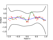
Figure 1: LEFT (Nominal setting): Example function (green) from SE kernel with length-scale 0.5 and RKHS norm 2, learned from 50 samples (red). Shown is the posterior mean (blue) and the uncertainty set from Theorem 1 for $\delta=0.01$. RIGHT (Misspecified setting): Example function from SE kernel with length-scale 0.2, learned with GPR using SE covariance function with length-scale 0.5. The violation of the uncertainty set is clearly visible.

Misspecified Setting

We now consider misspecification of the kernel, i.e. different kernels are used for generating the ground truth and as prior covariance function in GPR. As an example we use the SE kernel with different length-scales and use the ONB from (Steinwart and Christmann 2008, Section 4.4) to generate the RKHS functions. We start with the benign setting from Proposition 3, where the RKHS corresponding to the covariance function used in GPR contains the RKHS of the target function. For this, identical settings as in our first experiment above are used, but now we generate functions from the SE kernel with length-scale 0.5 and use the SE kernel with length-scale 0.2 in GPR. This corresponds to the benign setting according to Proposition 4. As expected, we find the same results as above, i.e. the uncertainty set fully contains the ground truth in all repetitions. Furthermore, the scalings $\beta_{50}$ are roughly of the same size as in the nominal case, cf. Table 2 (upper row).

Next, we investigate the problematic setting where the RKHS corresponding to the covariance function used in GPR does not contain the RKHS of the target function anymore. As an example we use again the SE kernel, but now with length-scale 0.2 for generating RKHS functions and the SE kernel with length-scale 0.5 for GPR. We found a considerable number of function instances where the bounds from Theorem 1 were violated with higher frequency than $\delta$. More precisely, for a given function the tube of width $\beta_{50}\sigma_{50}(x)$ around $\mu_{50}(x)$ does not fully contain the function in more than $\delta\times 10000$ of the learning instances. This happened for 2, 6, 12, 13 out of 50 functions for $\delta=0.1,0.01,0.001,0.0001$, respectively.

Interestingly, when performing this experiment using the standard approach of generating functions from the RKHS based on linear combinations of kernels, we did not find functions that violated the uncertainty bounds more often than prescribed. This reaffirmes our introductory remark that the method generating the test targets can lead to wrong judgements of the theoretical results.

The results of the previous two experiments indicate that a model misspecification of the kernel can be a problem and a robust result like Theorem 5 is necessary. Indeed, a repetition of the last experiment with the uncertainty set from Theorem 5 instead of Theorem 1 resulted in all functions being contained in the uncertainty set in all repetitions. An inspection of the average uncertainty set widths in Table 3 indicates some conservatism.

Table 1: $\beta_{50}$ in nominal setting (mean $\pm$ standard deviation over all repetitions)

$\delta$	0.1	0.01	0.001	0.0001
SE	$6.95\pm 0.04$	$7.39\pm 0.04$	$7.80\pm 0.03$	$8.19\pm 0.03$
Matern	$7.36\pm 0.04$	$7.78\pm 0.04$	$8.16\pm 0.04$	$8.53\pm 0.04$

Table 2: $\beta_{50}$ in the misspecified setting (mean $\pm$ standard deviation over all repetitions)

$\delta$	0.1	0.01	0.001	0.0001
Benign	$6.53\pm 0.038$	$6.97\pm 0.035$	$7.39\pm 0.033$	$7.77\pm 0.031$
Problematic	$6.11\pm 0.03$	$6.64\pm 0.03$	$7.11\pm 0.02$	$7.54\pm 0.02$

Table 3: Width of robust uncertainty set (mean $\pm$ SD of average width)

$\delta$	0.1	0.01	0.001	0.0001
Mean	$71.68\pm 5.36$	$73.79\pm 5.36$	$75.64\pm 5.37$	$77.33\pm 5.37$
SD	$6.54\pm 1.73$	$6.73\pm 1.78$	$6.91\pm 1.82$	$7.06\pm 1.86$

4.2 Control Example

We now show the usefulness of our results for robust control by applying it to a concrete, existing learning-based control method. Due to space constraints only a brief description of the example can be given here. For more details and discussions we refer to the supplementary material.

As an example, we choose the algorithm from (Soloperto et al. 2018) which is a learning-based Robust Model Predictive Control (RMPC) approach that comes with rigorous control-theoretic guarantees. We refer to (Rawlings, Mayne, and Diehl 2017, Chapter 3) for background on RMPC and to (Hewing et al. 2019) for a recent survey on related learning-based control methods. We follow (Soloperto et al. 2018) and consider the discrete-time system

$$\begin{bmatrix}x_{1}^{+}\\ x_{2}^{+}\end{bmatrix}=\begin{bmatrix}0.995&0.095\\ -0.095&0.900\end{bmatrix}\begin{bmatrix}x_{1}\\ x_{2}\end{bmatrix}+\begin{bmatrix}0.048\\ 0.95\end{bmatrix}u+\begin{bmatrix}0\\ -r(x_{2})\end{bmatrix}$$ (6)

modelling a mass-spring-damper system with some nonlinearity $r$ (this could be interpreted as a friction term). The goal is the stabilization of the origin subject to the state and control constraints $\mathbb{X}=[-10,10]\times[-10,10]$ and $\mathbb{U}=[-3,3]$, as well as minimizing a quadratic cost.

The approach from (Soloperto et al. 2018) performs this task by interpreting (13) as a linear system with disturbance, given by the nonlinearity $r$, whose graph is a-priori known to lie in the set $\mathbb{W}_{0}=[-10,10]\times[-7,7]$. The nonlinearity is assumed to be unknown and has to be learned from data. The RMPC algorithm requires as an input disturbance sets $\mathbb{W}(x)$ such that $\begin{pmatrix}0&-r(x_{2})\end{pmatrix}^{\top}\in\mathbb{W}(x)$ for all $x\in\mathbb{X}$, which are in turn used to generate tightened nominal constraints ensuring robust constraint satisfaction. Furthermore, the tighter the sets $\mathbb{W}(x)$ are, the better is the performance of the algorithm. We now randomly generate the function $r$ (which will be our ground truth) from the RKHS with kernel $k(x,x^{\prime})=4\exp\left(-\frac{(x-x^{\prime})^{2}}{2\times 0.8^{2}}\right)$ with RKHS norm 2. Following (Soloperto et al. 2018), we uniformly sample 100 partial states $x_{2}\in[-10,10]$, evaluate $r$ at these and add i.i.d. Gaussian noise with a standard deviation of 0.01 to it. The unknown function is then learned using GPR from this data set. Our results then lead to an uncertainty set of the form $\mathbb{W}(x)=[\mu_{100}(x_{2})-\beta_{100}\sigma_{100}(x_{2}),\mu_{100}(x_{2})+\beta_{100}\sigma_{100}(x_{2})],$ with $\beta_{100}$ from Theorem 1 for $\delta:=0.001$. In particular, with probability at least $1-\delta$ we can guarantee that $r(x_{2})\in\mathbb{W}(x)$ holds for all $x\in\mathbb{X}$.

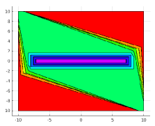
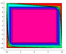
Figure 2: Tightened state constraint sets $\mathbb{Z}_{k}$ for $k=0,\ldots,9$. Computed from a-priori uncertainty set $\mathbb{W}_{0}$ (LEFT) and learned uncertainty sets $\mathbb{W}(x)$ (RIGHT).

Figure 2 shows the resulting tightened state constraints for an MPC horizon of 9. Clearly, the state constraint sets from the learned uncertainty sets are much larger. Furthermore, in contrast to previous work, we can guarantee that the RMPC controller using these tightened state constraints retains all control-theoretic guarantees with probability at least $1-\delta$. In the present case we can ensure state and control constraint satisfaction, input-to-state stability and convergence to a neighborhood of the origin, with probability at least $1-\delta$. This follows immediately from (Soloperto et al. 2018, Theorem 1), since the ground truth $r$ is covered by the uncertainty sets $\mathbb{W}(x)$ with this probability. Note that no changes to the existing RMPC scheme were necessary and the control-theoretic guarantees were retained with prescribed high probability.

5 Conclusion

We discussed the importance of frequentist uncertainty bounds for Gaussian Process Regression and improved existing results in this kind. By aiming only at a-posteriori bounds we were able to provide rigorous and practical uncertainty results. Our bounds can be explicitly evaluated and are sharp enough to be useful for concrete applications, as demonstrated with numerical experiments. Furthermore, we also introduced robust versions that work despite certain model mismatches, which is an important concern in real-world applications. We see the present work as a starting point for further developments, in particular, domain-specific versions of our results and more specific and less conservative robustness results.

Acknowledgments.

We would like to thank Sayak Ray Chowdhury and Tobias Holicki for helpful discussions, Steve Heim for useful comments on a draft of this work, and Raffaele Soloperto for providing the Matlab code from (Soloperto et al. 2018). Furthermore, we would like to thank the reviewers for their helpful and constructive feedback. Funded by Deutsche Forschungsgemeinschaft (DFG, German Research Foundation) under Germany’s Excellence Strategy - EXC 2075 – 390740016 and in part by the Cyber Valley Initiative. We acknowledge the support by the Stuttgart Center for Simulation Science (SimTech).

Supplementary material

In this supplementary material, we first give details on the corrections in this version. We then provide the detailed proofs in Section B that were omitted in the main paper, and further details on the numerical examples in Section B. Before this, we provide a straightforward and illustrative introduction to our results and their use in Section A.

Corrections

This version contains some corrections of the original work, which we now describe.

Unfortunately, there was a problem with constants in Theorem 1. In order to prove this result, we rely on the concentration inequality (Chowdhury and Gopalan 2017, Theorem 1), which requires that the nominal noise variance $\lambda$ in the GP regression is at least 1. In order to provide an uncertainty bound for all $\lambda>0$, we introduced a modified nominal variance $\bar{\lambda}$, but this object was not used correctly in the proof. In this version, we have repaired the issue, cf. Theorem 1 and its proof. All results that rely on it were changed accordingly (by using the correct formula for $\beta_{N}$). Among the results in this work, only a constant in Theorem 5 is affected and has also been corrected. Note that for $\lambda\geq 1$, we have $\bar{\lambda}=\lambda$, and the results as stated in the original version hold without requiring correction.

Second, the statement of Proposition 4 was imprecise. This result states that Theorem 1 holds also in a certain misspecified setting without change. However, since the operator norm of the inclusion map described in Proposition 3 is in general greater than 1, one has to use an RKHS norm that is valid in the misspecified setting. We have added a footnote to clarify this issue.

Appendix A A user-friendly overview

We provide in this section a simple tutorial overview of the approach. For simplicity, consider a scalar function on $D=[-10,10]$, generated from the RKHS of the Squared Exponential (SE) kernel with RKHS norm 2. A typical example looks as follows.

Next, assume we have a data set of input-output samples from the unknown target function. Since our bounds are rather flexible in the choice of the underlying concentration results, many common noise settings are supported. In particular, in Theorem 1 and 5 we use the powerful Theorem 1 from (Chowdhury and Gopalan 2017) which is compatible with (conditional) subgaussian martingale-difference noise. For demonstration purposes, we use in this simple example i.i.d. $\mathcal{N}(0,0.1)$ noise, resulting in the following data set with 100 data points.

Since we rely on standard Gaussian Process Regression (GPR), a large variety on modelling tools are available. In particular, since no additional assumption on the kernel (covariance function) are necessary later on, we can include additional prior knowledge in a systematic manner in the kernel. For example, linearly constrained constrained GPs (Jidling et al. 2017) or related approaches like (Geist and Trimpe 2020) could be used. In this simple example, we do not assume any additional structural and use the SE covariance function with length-scale 0.8 that has been used to generate the target function. However, we like to stress that this is only for demonstrative purposes. Everything would work with multivariate inputs or more general kernels. Furthermore, for simplicity we use the true noise variance. Again, this is for demonstrative purposes and general subgaussian noise would also work. This results in the following posterior GP. Note that the uncertainty set here is not in a frequentist sense, i.e., in general we cannot say with probability at least 2 SD it covers the ground truth.

Suppose now that we need tight frequentist uncertainty sets. This is a relevant scenario in many safe-critical applications, e.g., in robust learning-based control. First, we need to determine whether the nominal results (e.g., Theorem 1 in the main text) are applicable or a robust version is necessary. For simplicity, we work in the nominal setting, i.e. we use the SE kernel used to generate the ground truth. Next, we need a reasonable upper bound on the RKHS norm of the target function, as in related work like (Chowdhury and Gopalan 2017) and (Maddalena, Scharnhorst, and Jones 2020). Deriving such a bound from established prior knowledge (in particular, in engineering applications) is ongoing work, so here we simply use the true RKHS norm and a safety margin like in (Maddalena, Scharnhorst, and Jones 2020) (here we bound the norm by 3). Note that in contrast to heuristics that directly set a value for the scaling factor $\beta$, the RKHS norm bound has a concrete interpretation as a measure of complexity of the ground truth and hence is directly related to prior knowledge about the target function. We use $\delta=0.01$ in Theorem 1, resulting in the following uncertainty set.

Note that the uncertainty set covers the ground truth at least with probability $1-\delta=0.99$ w.r.t. the data generating process. This is exactly the guarantee needed for robust approaches. The latter are usually non-stochastic and hence any non-stochastic guarantees derived from the uncertainty set hold with the same high frequentist probability as the uncertainty set itself.

Appendix B Theory

B.1 Proof of Theorem 1

Following the proof of Theorem 2 from (Chowdhury and Gopalan 2017) we get for all $x\in D$ that

$$|f(x)-\mu_{N}(x)| =|f(x)-\boldsymbol{k}_{N}(x)^{T}(\boldsymbol{K}_{N}+\lambda\mathcal{I}_{N})^{-1}(\boldsymbol{f}_{N}+\boldsymbol{\epsilon}_{N})|$$ (7)

$$\leq|f(x)-\boldsymbol{k}_{N}(x)^{T}(\boldsymbol{K}_{N}+\lambda\mathcal{I}_{N})^{-1}\boldsymbol{f}_{N}|+|\boldsymbol{k}_{N}(x)^{T}(\boldsymbol{K}_{N}+\lambda\mathcal{I}_{N})^{-1}\boldsymbol{\epsilon}_{N}|$$

$$\leq\|f\|_{k}\sigma_{N}(x)+\frac{1}{\sqrt{\lambda}}\sigma_{N}(x)\sqrt{\boldsymbol{\epsilon}_{N}^{T}\boldsymbol{K}_{N}(\boldsymbol{K}_{N}+\lambda\mathcal{I}_{N})^{-1}\boldsymbol{\epsilon}_{N}}.$$

We furthermore have

$$\boldsymbol{K}_{N}(\boldsymbol{K}_{N}+\lambda\mathcal{I}_{N})^{-1} =\frac{\bar{\lambda}}{\lambda}\left(\frac{\bar{\lambda}}{\lambda}\right)^{-1}\boldsymbol{K}_{N}(\boldsymbol{K}_{N}+\lambda\mathcal{I}_{N})^{-1}$$

$$=\frac{\bar{\lambda}}{\lambda}\boldsymbol{K}_{N}\left(\left(\frac{\bar{\lambda}}{\lambda}\right)(\boldsymbol{K}_{N}+\lambda\mathcal{I}_{N})\right)^{-1}$$

$$=\frac{\bar{\lambda}}{\lambda}\boldsymbol{K}_{N}\left(\frac{\bar{\lambda}}{\lambda}\boldsymbol{K}_{N}+\bar{\lambda}\mathcal{I}_{N}\right)^{-1}$$

$$=\bar{\boldsymbol{K}}_{N}\left(\bar{\boldsymbol{K}}_{N}+\bar{\lambda}\mathcal{I}_{N}\right)^{-1},$$

where we defined $\bar{\boldsymbol{K}}_{N}=\frac{\bar{\lambda}}{\lambda}\boldsymbol{K}_{N}$. Since $\bar{\lambda}\geq 1$ and $\bar{\boldsymbol{K}}_{N}$ is positive definite, we can use Theorem 1 from (Chowdhury and Gopalan 2017) (applied to the kernel $\frac{\bar{\lambda}}{\lambda}k$ instead of $k$) to get that with probability at least $1-\delta$

$$\boldsymbol{\epsilon}_{N}^{T}\bar{\boldsymbol{K}}_{N}(\bar{\boldsymbol{K}}_{N}+\bar{\lambda}\mathcal{I}_{N})^{-1}\boldsymbol{\epsilon}_{N}\leq R\sqrt{\log\left(\operatorname{det}(\bar{\boldsymbol{K}}_{N}+\bar{\lambda}\mathcal{I}_{N})\right)-2\log(\delta)}\sigma_{N}(x)$$

for all $x\in D$. Because $\sigma_{N}$ does not depend on $\boldsymbol{\epsilon}_{N}$, we can use this in (7) and the result follows. ∎

B.2 Proof of Proposition 2

Let $x\in D$ be arbitrary, then

$$|f(x)-\mu_{N}(x)| =|f(x)-\boldsymbol{k}_{N}(x)^{T}(\boldsymbol{K}_{N}+\lambda\mathcal{I}_{N})^{-1}(\boldsymbol{f}_{N}+\boldsymbol{\epsilon}_{N})|$$

$$\leq|f(x)-\boldsymbol{k}_{N}(x)^{T}(\boldsymbol{K}_{N}+\lambda\mathcal{I}_{N})^{-1}\boldsymbol{f}_{N}|+|\boldsymbol{k}_{N}(x)^{T}(\boldsymbol{K}_{N}+\lambda\mathcal{I}_{N})^{-1}\boldsymbol{\epsilon}_{N}|.$$

Exactly as in the proof of Theorem 2 in (Chowdhury and Gopalan 2017) we have

$$|f(x)-\boldsymbol{k}_{N}(x)^{T}(\boldsymbol{K}_{N}+\lambda\mathcal{I}_{N})^{-1}\boldsymbol{f}_{N}|\leq B\sigma_{N}(x)$$

and since (use Cauchy-Schwarz)

$$|\boldsymbol{k}_{N}(x)^{T}(\boldsymbol{K}_{N}+\lambda\mathcal{I}_{N})^{-1}\boldsymbol{\epsilon}_{N}| \leq\|(\boldsymbol{K}_{N}+\lambda\mathcal{I}_{N})^{-1}\boldsymbol{k}_{N}(x)\|\|\boldsymbol{\epsilon}_{N}\|=\|(\boldsymbol{K}_{N}+\lambda\mathcal{I}_{N})^{-1}\boldsymbol{k}_{N}(x)\|\sqrt{\boldsymbol{\epsilon}_{N}^{T}\mathcal{I}_{N}\boldsymbol{\epsilon}_{N}}$$

we get from Theorem 2.1 in (Hsu et al. 2021) that

$$\mathbb{P}\left[\|\boldsymbol{\epsilon}_{N}\|^{2}\leq R^{2}(N+2\sqrt{N}\sqrt{\log(\frac{1}{\delta})}+2\log(\frac{1}{\delta}))\right]\geq 1-\delta$$

and the result follows. ∎

B.3 Proof of Theorem 5

Denote by $\tilde{\mu}_{N}$, $\tilde{\sigma}_{N}^{2}$, $\tilde{\boldsymbol{K}}_{N}$ the posterior mean, posterior variance and Gram matrix of the GP, but with $\tilde{k}$ as covariance function, and analogously $\tilde{\boldsymbol{k}}_{N}$. Let $x\in D$ be arbitrary, then we have

$$|f(x)-\mu_{N}(x)|\leq|f(x)-\tilde{\mu}_{N}(x)|+|\tilde{\mu}_{N}(x)-\mu_{N}(x)|.$$

Our strategy will be to bound the first term on the right-hand-side with Theorem 1 and then upper bound all resulting or remaining quantities by expressions involving only $k$ instead of $\tilde{k}$. As a preparation we first derive some elementary bounds that are frequently used later on. By assumption,

$$\|\tilde{\boldsymbol{k}}_{N}(x)-\boldsymbol{k}_{N}(x)\|=\sqrt{\sum_{i=1}^{N}(\tilde{k}(x,x_{i})-k(x,x_{i}))^{2}}\leq\sqrt{N}\tilde{\epsilon}$$ (8)

and hence (using the triangle inequality)

$$\|\tilde{\boldsymbol{k}}_{N}(x)\|\leq\|\boldsymbol{k}_{N}(x)\|+\|\tilde{\boldsymbol{k}}_{N}(x)-\boldsymbol{k}_{N}(x)\|\leq\|\boldsymbol{k}_{N}(x)\|+\sqrt{N}\tilde{\epsilon}.$$ (9)

Furthermore, since $\tilde{\boldsymbol{K}}_{N}$ is positive semidefinite

$$\|(\tilde{\boldsymbol{K}}_{N}+\lambda\mathcal{I}_{N})^{-1}\|=\lambda_{\text{max}}((\tilde{\boldsymbol{K}}_{N}+\lambda\mathcal{I}_{N})^{-1})=\frac{1}{\lambda_{\text{min}}(\tilde{\boldsymbol{K}}_{N}+\lambda\mathcal{I}_{N})}\leq\frac{1}{\lambda}$$

and hence together with the triangle inequality

$$\|(\tilde{\boldsymbol{K}}_{N}+\lambda\mathcal{I}_{N})^{-1}-(\boldsymbol{K}_{N}+\lambda\mathcal{I}_{N})^{-1}\|\leq\frac{1}{\lambda}+\|(\boldsymbol{K}_{N}+\lambda\mathcal{I}_{N})^{-1}\|.$$ (10)

Finally, using first the triangle inequality and then the submultiplicativity of the spectral norm we get

$$\|(\tilde{\boldsymbol{K}}_{N}+\lambda\mathcal{I}_{N})^{-1}\tilde{\boldsymbol{k}}_{N}(x)-(\boldsymbol{K}_{N}+\lambda\mathcal{I}_{N})^{-1}\boldsymbol{k}_{N}(x)\|$$

$$\hskip 28.45274pt\leq\|\left(\tilde{\boldsymbol{K}}_{N}+\lambda\mathcal{I}_{N})^{-1}-(\boldsymbol{K}_{N}+\lambda\mathcal{I}_{N})^{-1}\right)\tilde{\boldsymbol{k}}_{N}(x)\|+\|(\boldsymbol{K}_{N}+\lambda\mathcal{I}_{N})^{-1}(\tilde{\boldsymbol{k}}_{N}(x)-\boldsymbol{k}_{N}(x))\|$$

$$\hskip 28.45274pt\leq\|(\tilde{\boldsymbol{K}}_{N}+\lambda\mathcal{I}_{N})^{-1}-(\boldsymbol{K}_{N}+\lambda\mathcal{I}_{N})^{-1}\|\|\tilde{\boldsymbol{k}}_{N}(x)\|+\|(\boldsymbol{K}_{N}+\lambda\mathcal{I}_{N})^{-1}\|\|\tilde{\boldsymbol{k}}_{N}(x)-\boldsymbol{k}_{N}(x)\|$$

and hence from (8), (9), (10)

$$\|(\tilde{\boldsymbol{K}}_{N}+\lambda\mathcal{I}_{N})^{-1}\tilde{\boldsymbol{k}}_{N}(x)-(\boldsymbol{K}_{N}+\lambda\mathcal{I}_{N})^{-1}\boldsymbol{k}_{N}(x)\|\leq C_{N}(x)$$ (11)

with

$$C_{N}(x)=\left(\frac{1}{\lambda}+\|(\boldsymbol{K}_{N}+\lambda\mathcal{I}_{N})^{-1}\|\right)(\|\boldsymbol{k}_{N}(x)\|+\sqrt{N}\tilde{\epsilon})+\|(\boldsymbol{K}_{N}+\lambda\mathcal{I}_{N})^{-1}\|\sqrt{N}\tilde{\epsilon}$$

Now,

$$|\tilde{\mu}_{N}(x)-\mu_{N}(x)| =|\tilde{\boldsymbol{k}}_{N}(x)(\tilde{\boldsymbol{K}}_{N}+\lambda\mathcal{I}_{N})^{-1}\boldsymbol{y}_{N}-\boldsymbol{k}_{N}(x)(\boldsymbol{K}_{N}+\lambda\mathcal{I}_{N})^{-1}\boldsymbol{y}_{N}|$$

$$\leq\|(\tilde{\boldsymbol{K}}_{N}+\lambda\mathcal{I}_{N})^{-1}\tilde{\boldsymbol{k}}_{N}(x)+(\boldsymbol{K}_{N}+\lambda\mathcal{I}_{N})^{-1}\boldsymbol{k}_{N}(x)\|\|\boldsymbol{y}_{N}\|$$

$$\leq C_{N}(x)\|\boldsymbol{y}_{N}\|,$$

where we used Cauchy-Schwarz in the first inequality and (11) in the second. Using Theorem 1 we get that

$$\mathbb{P}\left[|\tilde{\mu}_{N}(x)-f(x)|\leq\tilde{\beta}_{N}\tilde{\sigma}_{N}(x)\>\forall N\in\mathbb{N},x\in D\right]\geq 1-\delta$$

where

$$\tilde{\beta}_{N}=B+\frac{R}{\sqrt{\lambda}}\sqrt{\log\left(\operatorname{det}(\bar{\lambda}/\lambda\tilde{\boldsymbol{K}}_{N}+\bar{\lambda}\mathcal{I}_{N})\right)-2\log(\delta)}.$$

Let $\lambda_{i}(\tilde{\boldsymbol{K}}_{N})$ be the $i$-th largest eigenvalue of $\tilde{\boldsymbol{K}}_{N}$, then we get from Weyl’s inequality and the definition of the Frobenius norm that

$$\lambda_{i}(\tilde{\boldsymbol{K}}_{N})\leq\lambda_{i}(\boldsymbol{K}_{N})+\|\tilde{\boldsymbol{K}}_{N}-\boldsymbol{K}_{N}\|\leq\lambda_{i}(\boldsymbol{K}_{N})+N\tilde{\epsilon},$$

and hence

$$\log\operatorname{det}\left(\frac{\bar{\lambda}}{\lambda}\tilde{\boldsymbol{K}}_{N}+\bar{\lambda}\mathcal{I}_{N}\right) =\log\left(\prod_{i=1}^{N}\lambda_{i}\left(\frac{\bar{\lambda}}{\lambda}\tilde{\boldsymbol{K}}_{N}+\bar{\lambda}\mathcal{I}_{N}\right)\right)$$

$$=\log\left(\prod_{i=1}^{N}\left(\frac{\bar{\lambda}}{\lambda}\lambda_{i}(\tilde{\boldsymbol{K}}_{N})+\bar{\lambda}\right)\right)$$

$$=\sum_{i=1}^{N}\log\left(\frac{\bar{\lambda}}{\lambda}\lambda_{i}(\tilde{\boldsymbol{K}}_{N})+\bar{\lambda}\right)$$

$$\leq\sum_{i=1}^{N}\log\left(\frac{\bar{\lambda}}{\lambda}\lambda_{i}(\boldsymbol{K}_{N})+\frac{\bar{\lambda}}{\lambda}N\tilde{\epsilon}+\bar{\lambda}\right)$$

$$=\log\operatorname{det}\left(\frac{\bar{\lambda}}{\lambda}\boldsymbol{K}_{N}+\left(\frac{\bar{\lambda}}{\lambda}N\tilde{\epsilon}+\bar{\lambda}\right)\mathcal{I}_{N}\right).$$

In particular,

$$\tilde{\beta}_{N}=B+\frac{R}{\sqrt{\lambda}}\sqrt{\log\left(\operatorname{det}(\bar{\lambda}/\lambda\tilde{\boldsymbol{K}}_{N}+\bar{\lambda}\mathcal{I}_{N})\right)-2\log(\delta)}\leq B+\frac{R}{\sqrt{\lambda}}\sqrt{\log\operatorname{det}\left(\frac{\bar{\lambda}}{\lambda}\boldsymbol{K}_{N}+\left(\frac{\bar{\lambda}}{\lambda}N\tilde{\epsilon}+\bar{\lambda}\right)\mathcal{I}_{N}\right)-2\log(\delta)}=:\bar{\beta}_{N}$$

Turning to the posterior variance, we get from the triangle inequality

$$\tilde{\sigma}_{N}^{2}(x) \leq\sigma_{N}^{2}(x)+|\sigma_{N}^{2}(x)-\tilde{\sigma}_{N}^{2}(x)|.$$

We continue with

$$|\sigma_{N}^{2}(x)-\tilde{\sigma}_{N}^{2}(x)| =|k(x,x)-\boldsymbol{k}_{N}(x)^{T}(\boldsymbol{K}_{N}+\lambda\mathcal{I}_{N})^{-1}\boldsymbol{k}_{N}(x)-\tilde{k}(x,x)+\tilde{\boldsymbol{k}}_{N}(x)^{T}(\tilde{\boldsymbol{K}}_{N}+\lambda\mathcal{I}_{N})^{-1}\tilde{\boldsymbol{k}}_{N}(x)|$$

$$\leq|k(x,x)-\tilde{k}(x,x)|+|(\tilde{\boldsymbol{k}}_{N}(x)-\boldsymbol{k}_{N}(x))^{T}(\tilde{\boldsymbol{K}}_{N}+\lambda\mathcal{I}_{N})^{-1}\tilde{\boldsymbol{k}}_{N}(x)|$$

$$\hskip 28.45274pt+|\boldsymbol{k}_{N}(x)^{T}((\tilde{\boldsymbol{K}}_{N}+\lambda\mathcal{I}_{N})^{-1}\tilde{\boldsymbol{k}}_{N}(x)-(\boldsymbol{K}_{N}+\lambda\mathcal{I}_{N})^{-1}\boldsymbol{k}_{N}(x))|$$

$$\leq|k(x,x)-\tilde{k}(x,x)|+\|\tilde{\boldsymbol{k}}_{N}(x)-\boldsymbol{k}_{N}(x)\|\|(\tilde{\boldsymbol{K}}_{N}+\lambda\mathcal{I}_{N})^{-1}\tilde{\boldsymbol{k}}_{N}(x)\|$$

$$\hskip 28.45274pt+\|\boldsymbol{k}_{N}(x)\|\|(\tilde{\boldsymbol{K}}_{N}+\lambda\mathcal{I}_{N})^{-1}\tilde{\boldsymbol{k}}_{N}(x)-(\boldsymbol{K}_{N}+\lambda\mathcal{I}_{N})^{-1}\boldsymbol{k}_{N}(x)\|$$

$$\leq\tilde{\epsilon}+\sqrt{N}\tilde{\epsilon}\|(\boldsymbol{K}_{N}+\lambda\mathcal{I}_{N})^{-1}\boldsymbol{k}_{N}(x)\|+(\sqrt{N}\tilde{\epsilon}+\|\boldsymbol{k}_{N}(x)\|)C_{N}(x)=S^{2}_{N}(x),$$

where we used the triangle inequality again in the first inequality, Cauchy-Schwarz in the second inequality and finally (8), (9), (10) together with

$$\|(\tilde{\boldsymbol{K}}_{N}+\lambda\mathcal{I}_{N})^{-1}\tilde{\boldsymbol{k}}_{N}(x)\| \leq\|(\boldsymbol{K}_{N}+\lambda\mathcal{I}_{N})^{-1}\boldsymbol{k}_{N}(x)\|+\|(\tilde{\boldsymbol{K}}_{N}+\lambda\mathcal{I}_{N})^{-1}\tilde{\boldsymbol{k}}_{N}(x)-(\boldsymbol{K}_{N}+\lambda\mathcal{I}_{N})^{-1}\boldsymbol{k}_{N}(x)\|$$

$$\leq\|(\boldsymbol{K}_{N}+\lambda\mathcal{I}_{N})^{-1}\boldsymbol{k}_{N}(x)\|+C_{N}(x)$$

Putting everything together, we find that with probability at least $1-\delta$

$$|\mu_{N}(x)-f(x)|\leq C_{N}(x)\|\boldsymbol{y}_{N}\|+\tilde{\beta}_{N}\tilde{\sigma}_{N}(x)$$

and therefore, using the upper bounds on $\tilde{\beta}_{N}$ and $\tilde{\sigma}_{N}(x)$ derived above, that with probability at least $1-\delta$

$$|\mu_{N}(x)-f(x)|\leq B_{N}(x)$$

where

$$B_{N}(x)=C_{N}(x)\|\boldsymbol{y}_{N}\|+\bar{\beta}_{N}\sqrt{\sigma_{N}^{2}(x)+\tilde{\epsilon}+\sqrt{N}\tilde{\epsilon}\|(\boldsymbol{K}_{N}+\lambda\mathcal{I}_{N})^{-1}\boldsymbol{k}_{N}(x)\|+(\sqrt{N}\tilde{\epsilon}+\|\boldsymbol{k}_{N}(x)\|)C_{N}(x)}$$

∎

B.4 An alternative robustness result

The proof of Theorem 5 can be easily adapted to other nominal bounds. In order to illustrate this, we now state and prove a robust version of Proposition 2.

Proposition.

Consider the situation of Proposition 2, but this time assume that the target function $f$ is from the RKHS $(\tilde{H},\|\cdot\|_{\tilde{k}})$ of a different kernel $\tilde{k}$ such that still $\|f\|_{\tilde{k}}\leq B$ and $\sup_{x,x^{\prime}\in D}|k(x,x^{\prime})-\tilde{k}(x,x^{\prime})|\leq\tilde{\epsilon}$ for some $\tilde{\epsilon}\geq 0$. We then have for any $\delta\in(0,1)$ with

$$\tilde{\eta}=R(\|(\boldsymbol{K}_{N}+\lambda\mathcal{I}_{N})^{-1}\boldsymbol{k}_{N}(x)\|+C_{N}(x))\sqrt{N+2\sqrt{N}\sqrt{\log(\frac{1}{\delta})}+2\log(\frac{1}{\delta})}$$

that

$$\mathbb{P}\left[|\mu_{N}(x)-f(x)|\leq B\sqrt{\sigma^{2}_{N}(x)+S_{N}^{2}(x)}+C_{N}(x)\|\boldsymbol{y}_{N}\|+\tilde{\eta}_{N}(x)\>\forall x\in D\right]\geq 1-\delta$$

where $C_{N}(x)$ and $S^{2}_{N}(x)$ are defined in the main text by (4) and (5), respectively.

Proof.

Let $x\in D$ be arbitrary, then we have

$$|f(x)-\mu_{N}(x)|\leq|f(x)-\tilde{\mu}_{N}(x)|+|\tilde{\mu}_{N}(x)-\mu_{N}(x)|.$$

The second term can be upper bounded by $C_{N}(x)\|\boldsymbol{y}_{N}\|$ as in the proof of Theorem 5. Using Proposition 2 we have that with probability at least $1-\delta$ for all $x\in D$

$$|\tilde{\mu}_{N}(x)-f(x)|\leq B\tilde{\sigma}_{N}(x)+R\|(\tilde{\boldsymbol{K}}_{N}+\lambda\mathcal{I}_{N})^{-1}\tilde{\boldsymbol{k}}_{N}(x)\|\sqrt{N+2\sqrt{N}\sqrt{\log(\frac{1}{\delta})}+2\log(\frac{1}{\delta})}$$

From the proof of Theorem 5 we have

$$|\sigma_{N}^{2}(x)-\tilde{\sigma}_{N}^{2}(x)|\leq S^{2}_{N}(x)$$

and

$$\|(\tilde{\boldsymbol{K}}_{N}+\lambda\mathcal{I}_{N})^{-1}\tilde{\boldsymbol{k}}_{N}(x)\|C_{N}(x)$$

and the result follows. ∎

Appendix C Numerical experiments

We now provide more details on the numerical experiments as well as additional remarks and results.

C.1 Generating functions from an RKHS

For the numerical experiments we need to generate ground truths, i.e. we need to randomly generate functions belonging to the RKHS of a given kernel. A generic approach is to use the pre-RKHS of the kernel which is contained (even densely w.r.t. the kernel norm) in the actual RKHS, cf. (Steinwart and Christmann 2008, Theorem 4.21) for details. Let $X$ be a set and $k$ a kernel on $X$. For any $N\in\mathbb{N}$, $x_{1},\ldots,x_{N}\in X$ and $\boldsymbol{\alpha}\in\mathbb{R}^{N}$ the function defined by

$$x\mapsto\sum_{n=1}^{N}\alpha_{n}k(x_{n},x)$$

is contained in the (unique) RKHS corresponding to $k$ and has RKHS norm $\sqrt{\boldsymbol{\alpha}^{T}\boldsymbol{K}\boldsymbol{\alpha}}$, where $\boldsymbol{K}=(k(x_{i},x_{j}))_{i,j=1,\ldots,N}$ is the corresponding Gram matrix. It is hence possible to generate an RKHS function $f$ of prescribed RKHS norm $B$ by randomly sampling inputs $x_{1},\ldots,x_{N}\in X$ and coefficients $\tilde{\alpha}\in\mathbb{R}^{N}$ and setting

$$f(x)=\sum_{n=1}^{N}\alpha_{n}k(x_{n},x)$$ (12)

where $\boldsymbol{\alpha}=\frac{B}{\sqrt{\boldsymbol{\alpha}^{T}\boldsymbol{K}\boldsymbol{\alpha}}}\tilde{\boldsymbol{\alpha}}$. Of course, $f$ can only be evaluated at finitely many points $\tilde{X}\subseteq X$.

More concretely, we fix a finite evaluation grid $\tilde{X}\subseteq X$, choose uniformely a number $N\in[N_{\text{min}},N_{\text{max}}]\cap\mathbb{N}$, choose uniformely $N$ pairwise different points $x_{1},\ldots,x_{N}\in\tilde{X}$, sample $\tilde{\alpha}_{i}\sim\mathcal{N}(0,\sigma_{f}^{2})$ and apply the construction (12). For precise choices of the parameters are given below.

We would like to point out an important aspect. This article is concerned with frequentist results, i.e., there is a ground truth from a collection of possible ground truths and the results have to hold for each of these possible ground truths. In particular, even if a ground truth might be considered pathological, the results have to hold if they are to be considered rigorous. This aspect is important for numerical experiments, especially when trying to assess the conservatism of a result. In our setting it might happen that the results seem very conservative for functions that are randomly generated in a certain fashion, but there are RKHS functions (which might be difficult to generate) for which the results might be sharp. Let us illustrate this point with the Gaussian kernel. We use a uniform grid of 1000 points from $[-1,1]$ together with the Gaussian kernel with length scale 0.2. For the pre-RKHS approach we use $N_{\text{min}}=5$ and $N_{\text{max}}=200$ and $\sigma_{f}^{2}=1$. As an alternative, we use the ONB described in (Steinwart and Christmann 2008, Section 4.4) and consider only the first 50 basis functions from (Steinwart and Christmann 2008, Equation (4.35)) for numerical reasons. We first select the number of basis functions $N$ to use uniformely between 5 and 50 and then choose $N$ such functions uniformely. As coefficients we sample $\alpha_{i}\sim\mathcal{N}(0,1)$ i.i.d. for $i=1,\ldots,N$ and normalize (w.r.t. to $\ell_{2}$-norm) and multiply by the targeted RKHS norm. For both the pre-RKHS approach and the ONB approach we use $\|\cdot\|_{k}=2$ and sample 4 functions each. The result is shown in Figure 3.

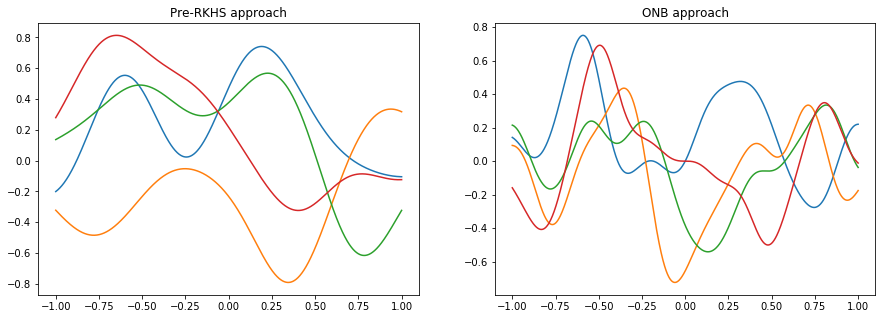
Figure 3: Illustrating sampling from the Gaussian kernel with the pre-RKHS method (left) and with an explicit ONB (right). Details are provided in the text.

Clearly, the resulting functions have a different shape, despite having the same RKHS norm with respect to the same kernel. In particular, the functions generated using the ONB approach seem to make sharper turns.

We like to stress that this strongly suggests that in a frequentist setting one has to be careful with statements about the conservatism of a proposed bound or method that are based purely on empirical observations. It might be that the method for generating ground truths has a certain bias, i.e. has a tendency to produce only ground truths from a certain region of the space of all ground truths.

C.2 Details on experiments with synthetic data

Unless otherwise stated, we use $[-1,1]$ as the input set and consider a uniform grid of 1000 points for function evaluations. For the pre-RKHS approach we use $N_{\text{min}}=5$ and $N_{\text{max}}=200$ and $\sigma_{f}^{2}=1$ in all experiments.

Unless otherwise stated, in each experiment we sample 50 RKHS functions as ground truth. For each ground truth we generate 10000 training sets by randomly sampling 50 input points uniformly from the 1000 evaluation points and add i.i.d. zero-mean normal noise with SD 0.5. For each training set we run Gaussian Process Regression (which we call a learning instance) and determine the uncertainty set for a specific setting (evaluated again at the 1000 evaluation points). We consider a learning instance a failure if the uncertainty set does not fully cover the ground truth at all 1000 evaluation points.

For convenience, each experiment has a tag with prefix exp_.

Testing the nominal bound

Here we use the SE kernel with length scale 0.2 (exp_1_1_a) and the Matern kernel with length scale 0.2 and $\nu=1.5$ (exp_1_1_b). We generate RKHS functions of RKHS norm 2 using the pre-RKHS approach and use the same kernel for generating the ground truth and running GPR. The nominal noise level of GPR is set to $\lambda=0.5$. The uncertainty set is generated using Theorem 1 with $B=2$, $R=0.5$ and $\delta=0.1,0.01,0.001,0.0001$. As already reported in the main text, a violation of the uncertainty set was found in no instance (i.e. for all 50 RKHS functions and each of the 10000 learning instances). The mean of the scalings $\beta_{50}$ (together with 1 SD, average is over all 50 RKHS functions and all learning instances) is shown in Table 1 in the main text.

Exploring conservatism

In order to explore the potential conservatism of Theorem 1 we repeated the previous experiments with $\delta=0.01$ and replaced $\beta_{50}$ by 20 equidistant scalings between 2 and $\beta_{50}$. We used this changed setup for the SE kernel (exp_1_2_a), Matern kernel (exp_1_2_b) and SE kernel together with the ONB sampling approach (exp_1_2_c). Whereas for the Matern kernel also the heuristic $\beta=2$ works for this example (still no uncertainty set violations), the situation is rather different for the SE kernel. As shown in Figure 4 for $\beta$ close to 2 the frequency of uncertainty violations is much higher than 0.01, in particular for the case of sampling from the ONB.

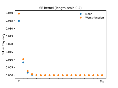
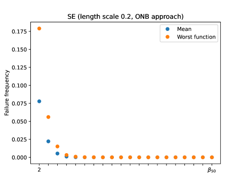
Figure 4: Exploring conservatism of Theorem 1. For each target function and learning instance 20 different uncertainty sets are tested. Each such uncertainty is generated from Theorem 1 by replacing $\beta_{50}$ by $\beta=2,\ldots,\beta_{50}$ (equidistant). Worst function means the highest failure frequency among all 50 target functions for the particular scaling. Ground truths sampled with pre-RKHS approach (left) and ONB approach (right).

Misspecified kernel, benign setting

We now consider model misspecification. We repeat the first experiment exp_1_1_a, but now generate RKHS functions from the SE kernel with lengthscale 0.5 and use the SE kernel with lengthscale 0.2 in GPR (exp_1_3_a). As discussed in the main text, Proposition 4 indicates that this is a benign form of model misspecification. Indeed, similar to the case of the correct kernel we find no uncertainty set violation and similar scalings. The corresponding scalings $\beta_{50}$ are reported in Table 2 (upper row) in the main text (only for ONB sampling approach, no significant difference compared to pre-RKHS approach).

Misspecified kernel, problematic setting

We repeat the previous experiment exp_1_3_a, but now generate RKHS functions from the SE kernel with lengthscale 0.2 and use the SE kernel with lengthscale 0.5 in GPR. We use both the pre-RKHS approach (exp_1_4_a) and the ONB approach (exp_1_4_b). The resulting scalings are reported in Table 2 (lower row) in the main text, again only for the ONB sampling approach. Interestingly, when using the pre-RKHS sampling approach no uncertainty set violation could be found, but for the ONB sampling we found some target function for which the uncertainty violation was higher than the prescribed $\delta$.

Robust result for misspecified setting

Finally, we repeat Experiment exp_1_4_b from the previous paragraph, but now using Theorem 5 instead of Theorem 1. We find no violation of the uncertainty set (over all 50 functions tested, all 10000 learning instances for each function and all $\delta$ tested). Since now the width of the uncertainty set is not a constant rescaling of the posterior standard deviation anymore, we report the mean (over all 50 functions and each of the 10000 learning instances) of the average width (over the input space) of the uncertainty sets ($\pm$ SD w.r.t. averaging over all 50 functions and each of the 10000 learning instances) and the SD (w.r.t. to averaging over the input space), $\pm$ SD w.r.t. averaging over all 50 functions and each of the 10000 learning instances, in Table 3 in the main text.

Reproducibility and computational complexity

All numerical experiments in this section were implemented with Python 3.8.3 (together with Numpy 1.18.1) and run on a Intel(R) Xeon(R) CPU E5-1680 v4 with 3.40GHz and 78 GiB memory (using Ubuntu 18.04.3 LTS). We used the joblib library (version 0.15.1) with $n\_jobs=14$ and used the Gaussian Process Regression implementation from scikit-learn, version 0.22.1. Each experiment took less than 5 minutes and required less than 1.5GiB memory (monitored using htop). Note that all experiments can easily be up and down scaled, depending on the available hardware. The code used for the experiments and figures can be found at https://github.com/Data-Science-in-Mechanical-Engineering/UncertaintyBounds21.

C.3 Control example

We now provide more details on the control example from Section 4.2.

Background

For convenience we now provide a cursory overview of background material from control theory. We can only provide a sketch and refer to standard textbooks for more details, e.g. (Åström and Murray 2010) for a general introduction to control and (Rawlings, Mayne, and Diehl 2017) for a comprehensive introduction to MPC.

A common goal in control is feedback stabilization under state and input constraints. Consider a discrete-time dynamical system (or control system) described by

$$x_{+}=f(x,u)$$

with state space $X$, input space $U$ and transition function $f:X\times U\rightarrow X$. For simplicity assume that $X=\mathbb{R}^{n}$, $U=\mathbb{R}^{m}$ and that $f(0,0)=0$, i.e., $(0,0)$ is an equilibrium. Furthermore, consider state constraints $\mathbb{X}\subseteq X$ and input constraints $\mathbb{U}\subseteq U$. Feedback stabilization amounts now to finding a map $\mu:X\rightarrow U$ such that $x_{\ast}=0$ is an asymptotically stable equilibrium for the resulting closed loop system described by

$$x_{+}=f(x,\mu(x)),$$

and all resulting state-input trajectories are contained in the constraint set $\mathbb{X}\times\mathbb{U}$. Note that this requires restriction of the set of possible initial values.

In many applications not only stability, but also a form of optimality is required from the control system. For example, assume that being in state $x$ and applying input $u$ incurs a cost of $\ell(x,u)$. If the control system is run for a long time, then we would like a feedback $\mu$ that not only stabilizes the system, but also incurs a small infinite horizon cost

$$\sum_{n=0}^{\infty}\ell(x(n),\mu(x(n))),$$

where $x(n)$ is the resulting state trajectory.

One common methodology for dealing with state constraints and optimal control tasks is MPC. If the system is in state $x$, MPC solves a finite horizon open loop problem, i.e. it determines a sequence $u(0),\ldots,u(N-1)$ of admissible input values that minimize some cost criterion. Only the first input $u(0)$ is applied to the system and this process is repeated at the next time instance. There is a comprehensive theory available on how to design the open loop optimal control problem solved in each instance, in order to achieve desired closed loop properties. For details we refer to Chapters 1 and 2 in (Rawlings, Mayne, and Diehl 2017).

In many applications a control system has to deal with disturbances. Frequently the disturbances can be modelled in an additive manner, i.e. we have a control system of the form

$$x_{+}=f(x,u)+w,$$

where $w\in\mathbb{W}\subseteq\mathbb{R}^{n}$ is an external disturbance. The feedback stabilization problem under constraints can now be adapted to this setting, resulting in robust feedback stabilization under constraints. The goal is now to find a feedback that ensures constraint satisfaction and stabilizes the origin in a relaxed sense (which depends on the size of the disturbance set $\mathbb{W}$). Furthermore, even in this more challenging situation one might have to deal with additional cost criterions.

MPC can be adapted to the setting with disturbances. The key idea of most approaches is to solve a constrained open loop optimal control problem where the constraints are tightened. The intuition is that even the worst case disturbance cannot throw the system out of the allowed state-input set. It is clear that this requires sufficiently small bounds on the size of the disturbances. For more details we refer to Chapter 3 in (Rawlings, Mayne, and Diehl 2017).

Details on the example

The control example in the main text is from Section 6 in (Soloperto et al. 2018). It consists of the following system

$$\begin{bmatrix}x_{1}^{+}\\ x_{2}^{+}\end{bmatrix}=\begin{bmatrix}0.995&0.095\\ -0.095&0.900\end{bmatrix}\begin{bmatrix}x_{1}\\ x_{2}\end{bmatrix}+\begin{bmatrix}0.048\\ 0.95\end{bmatrix}u+\begin{bmatrix}0\\ -r(x_{2})\end{bmatrix}$$ (13)

modelling a mass-spring-damper system with some nonlinearity $r$ (this could be interpreted as a friction term). As described in the main text, we replaced the Stribeck friction curve used by (Soloperto et al. 2018) with a synthetic nonlinearity generated from a known RKHS. Furthermore, the nonlinearity is assumed to be unknown and has to be learned from data. The control goal is the stabilization of the origin subject to the state and control constraints $\mathbb{X}=[-10,10]\times[-10,10]$ and $\mathbb{U}=[-3,3]$, as well as minimizing a quadratic cost $\ell(x,u)=10\|x\|+\|u\|$.

The RMPC approach from(Soloperto et al. 2018) performs this task by interpreting (13) as a linear system with disturbance, given by the nonlinearity $r$, whose graph is a-priori known to lie in the set $\mathbb{W}_{0}=[-10,10]\times[-7,7]$. The RMPC algorithm requires as an input disturbance sets $\mathbb{W}(x)$ such that $\begin{pmatrix}0&-r(x_{2})\end{pmatrix}^{\top}\in\mathbb{W}(x)$ for all $x\in\mathbb{X}$, which are in turn used to generate tightened nominal constraints ensuring robust constraint satisfaction. Furthermore, the tighter the sets $\mathbb{W}(x)$ are, the better is the performance of the algorithm, cf. Chapter 3 in (Rawlings, Mayne, and Diehl 2017) for an in-depth discussion.

We now describe the learning part of this example in more detail: The nonlinearity $r$ (which will be our ground truth) is sampled from the RKHS of the SE kernel

$$k(x,x^{\prime})=4\exp\left(-\frac{(x-x^{\prime})^{2}}{2\times 0.8^{2}}\right)$$

with RKHS norm 2. Following (Soloperto et al. 2018), we uniformly sample 100 partial states $x_{2}\in[-10,10]$, evaluate $r$ at these and add i.i.d. Gaussian noise with a standard deviation of 0.01 to it. The unknown function is then learned using GPR (using the nominal setting, i.e. with known $k$) from this data set. Theorem 1 then leads to an uncertainty set of the form $\mathbb{W}(x)=[\mu_{100}(x_{2})-\beta_{100}\sigma_{100}(x_{2}),\mu_{100}(x_{2})+\beta_{100}\sigma_{100}(x_{2})],$ where we use $\delta:=0.001$. In particular, with probability at least $1-\delta$ we can guarantee that $r(x_{2})\in\mathbb{W}(x)$ holds for all $x\in\mathbb{X}$. The situation is displayed in Figure 5.

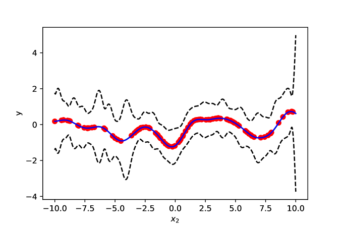
Figure 5: Example nonlinearity. From the target function (blue solid line) 100 samples with noise (red dots) are sampled, which are used to get the uncertainty sets (dashed black lines).

In order to follow (Soloperto et al. 2018) as closely as possible, we exported the learning results and used the original Matlab script to compute $\mathbb{Z}_{k}$ (provided by R. Soloperto). In order to save computation time, we decided to use a $50\times 50$ state space grid and an MPC horizon of 9.

The RMPC comes with deterministic guarantees. In particular, if the uncertainty is contained in the uncertainty sets, then the RMPC controller ensures constrained satisfaction and convergence to a neighborhood of the origin, as well as a form of Input-to-State stability, cf. Theorem 1 in (Soloperto et al. 2018). Since we can guarantee that the true uncertainty is covered by the uncertainty sets with probability $1-\delta$ by Theorem 1, the deterministic guarantees hold with at least the same probability.

References

- Abbasi-Yadkori (2013) Abbasi-Yadkori, Y. 2013. Online learning for linearly parametrized control problems. Ph.D. thesis, University of Alberta.
- Andersen and Chen (2020) Andersen, M. S.; and Chen, T. 2020. Smoothing Splines and Rank Structured Matrices: Revisiting the Spline Kernel. SIAM Journal on Matrix Analysis and Applications 41(2): 389–412.
- Åström and Murray (2010) Åström, K. J.; and Murray, R. M. 2010. Feedback systems: an introduction for scientists and engineers. Princeton university press.
- Beckers, Umlauft, and Hirche (2018) Beckers, T.; Umlauft, J.; and Hirche, S. 2018. Mean square prediction error of misspecified Gaussian process models. In 2018 IEEE Conference on Decision and Control (CDC), 1162–1167. IEEE.
- Berkenkamp (2019) Berkenkamp, F. 2019. Safe Exploration in Reinforcement Learning: Theory and Applications in Robotics. Ph.D. thesis, ETH Zurich.
- Berkenkamp et al. (2016) Berkenkamp, F.; Moriconi, R.; Schoellig, A. P.; and Krause, A. 2016. Safe learning of regions of attraction for uncertain, nonlinear systems with gaussian processes. In 2016 IEEE 55th Conference on Decision and Control (CDC), 4661–4666. IEEE.
- Berkenkamp, Schoellig, and Krause (2016) Berkenkamp, F.; Schoellig, A. P.; and Krause, A. 2016. Safe controller optimization for quadrotors with Gaussian processes. In 2016 IEEE International Conference on Robotics and Automation (ICRA), 491–496. IEEE.
- Berkenkamp et al. (2017) Berkenkamp, F.; Turchetta, M.; Schoellig, A.; and Krause, A. 2017. Safe model-based reinforcement learning with stability guarantees. In Advances in neural information processing systems, 908–918.
- Berlinet and Thomas-Agnan (2011) Berlinet, A.; and Thomas-Agnan, C. 2011. Reproducing kernel Hilbert spaces in probability and statistics. Springer Science & Business Media.
- Calandriello et al. (2019) Calandriello, D.; Carratino, L.; Lazaric, A.; Valko, M.; and Rosasco, L. 2019. Gaussian Process Optimization with Adaptive Sketching: Scalable and No Regret. In Conference on Learning Theory, 533–557.
- Chen and Andersen (2020) Chen, T.; and Andersen, M. 2020. On Semiseparable Kernels and Efficient Computation of Regularized System Identification and Function Estimation. IFAC-V 2020 .
- Chowdhury and Gopalan (2017) Chowdhury, S. R.; and Gopalan, A. 2017. On Kernelized Multi-armed Bandits. In International Conference on Machine Learning, 844–853.
- Dong et al. (2017) Dong, K.; Eriksson, D.; Nickisch, H.; Bindel, D.; and Wilson, A. G. 2017. Scalable log determinants for Gaussian process kernel learning. In Advances in Neural Information Processing Systems, 6327–6337.
- Geist and Trimpe (2020) Geist, A. R.; and Trimpe, S. 2020. Learning Constrained Dynamics with Gauss Principle adhering Gaussian Processes. In Proceedings of the 2nd Conference on Learning for Dynamics and Control, 225–234.
- Han, Malioutov, and Shin (2015) Han, I.; Malioutov, D.; and Shin, J. 2015. Large-scale log-determinant computation through stochastic Chebyshev expansions. In International Conference on Machine Learning, 908–917.
- Helwa, Heins, and Schoellig (2019) Helwa, M. K.; Heins, A.; and Schoellig, A. P. 2019. Provably robust learning-based approach for high-accuracy tracking control of lagrangian systems. IEEE Robotics and Automation Letters 4(2): 1587–1594.
- Hewing et al. (2019) Hewing, L.; Wabersich, K. P.; Menner, M.; and Zeilinger, M. N. 2019. Learning-Based Model Predictive Control: Toward Safe Learning in Control. Annual Review of Control, Robotics, and Autonomous Systems 3.
- Hsu et al. (2012) Hsu, D.; Kakade, S.; Zhang, T.; et al. 2012. A tail inequality for quadratic forms of subgaussian random vectors. Electronic Communications in Probability 17.
- Huggins et al. (2019) Huggins, J. H.; Campbell, T.; Kasprzak, M.; and Broderick, T. 2019. Scalable Gaussian Process Inference with Finite-data Mean and Variance Guarantees. In The 22nd International Conference on Artificial Intelligence and Statistics, 796–805.
- Jain et al. (2018) Jain, A.; Nghiem, T.; Morari, M.; and Mangharam, R. 2018. Learning and control using Gaussian processes. In 2018 ACM/IEEE 9th International Conference on Cyber-Physical Systems (ICCPS), 140–149. IEEE.
- Jidling et al. (2017) Jidling, C.; Wahlström, N.; Wills, A.; and Schön, T. B. 2017. Linearly constrained Gaussian processes. In Advances in Neural Information Processing Systems, 1215–1224.
- Kanagawa et al. (2018) Kanagawa, M.; Hennig, P.; Sejdinovic, D.; and Sriperumbudur, B. K. 2018. Gaussian processes and kernel methods: A review on connections and equivalences. arXiv preprint arXiv:1807.02582 .
- Kandasamy, Schneider, and Póczos (2015) Kandasamy, K.; Schneider, J.; and Póczos, B. 2015. High dimensional Bayesian optimisation and bandits via additive models. In International Conference on Machine Learning, 295–304.
- Kocijan (2016) Kocijan, J. 2016. Modelling and control of dynamic systems using Gaussian process models. Springer.
- Koller et al. (2018) Koller, T.; Berkenkamp, F.; Turchetta, M.; and Krause, A. 2018. Learning-based model predictive control for safe exploration. In 2018 IEEE Conference on Decision and Control (CDC), 6059–6066. IEEE.
- Lange-Hegermann (2018) Lange-Hegermann, M. 2018. Algorithmic linearly constrained Gaussian processes. In Advances in Neural Information Processing Systems, 2137–2148.
- Lederer, Umlauft, and Hirche (2019) Lederer, A.; Umlauft, J.; and Hirche, S. 2019. Uniform Error Bounds for Gaussian Process Regression with Application to Safe Control. In Advances in Neural Information Processing Systems, 657–667.
- Liu et al. (2018) Liu, M.; Chowdhary, G.; Da Silva, B. C.; Liu, S.-Y.; and How, J. P. 2018. Gaussian processes for learning and control: A tutorial with examples. IEEE Control Systems Magazine 38(5): 53–86.
- Maddalena, Scharnhorst, and Jones (2020) Maddalena, E. T.; Scharnhorst, P.; and Jones, C. N. 2020. Deterministic error bounds for kernel-based learning techniques under bounded noise. arXiv preprint arXiv:2008.04005 .
- Murphy (2012) Murphy, K. P. 2012. Machine learning: a probabilistic perspective. MIT press.
- Rasmussen and Williams (2006) Rasmussen, C. E.; and Williams, C. K. 2006. Gaussian Processes for Machine Learning. The MIT Press.
- Rawlings, Mayne, and Diehl (2017) Rawlings, J. B.; Mayne, D. Q.; and Diehl, M. 2017. Model predictive control: theory, computation, and design, volume 2. Nob Hill Publishing Madison, WI.
- Shahriari et al. (2015) Shahriari, B.; Swersky, K.; Wang, Z.; Adams, R. P.; and De Freitas, N. 2015. Taking the human out of the loop: A review of Bayesian optimization. Proceedings of the IEEE 104(1): 148–175.
- Skogestad and Postlethwaite (2007) Skogestad, S.; and Postlethwaite, I. 2007. Multivariable feedback control: analysis and design, volume 2. Wiley New York.
- Soloperto et al. (2018) Soloperto, R.; Müller, M. A.; Trimpe, S.; and Allgöwer, F. 2018. Learning-based robust model predictive control with state-dependent uncertainty. IFAC-PapersOnLine 51(20): 442–447.
- Srinivas et al. (2010) Srinivas, N.; Krause, A.; Kakade, S.; and Seeger, M. 2010. Gaussian process optimization in the bandit setting: no regret and experimental design. In Proceedings of the 27th International Conference on International Conference on Machine Learning, 1015–1022.
- Steinwart and Christmann (2008) Steinwart, I.; and Christmann, A. 2008. Support vector machines. Springer Science & Business Media.
- Szabó et al. (2015) Szabó, B.; Van Der Vaart, A. W.; van Zanten, J.; et al. 2015. Frequentist coverage of adaptive nonparametric Bayesian credible sets. The Annals of Statistics 43(4): 1391–1428.
- Umlauft et al. (2017) Umlauft, J.; Beckers, T.; Kimmel, M.; and Hirche, S. 2017. Feedback linearization using Gaussian processes. In 2017 IEEE 56th Annual Conference on Decision and Control (CDC), 5249–5255. IEEE.
- Wang, Tuo, and Jeff Wu (2019) Wang, W.; Tuo, R.; and Jeff Wu, C. 2019. On prediction properties of kriging: Uniform error bounds and robustness. Journal of the American Statistical Association 1–27.