acorn: Adaptive Coordinate Networks for Neural Scene Representation

Abstract.

Neural representations have emerged as a new paradigm for applications in rendering, imaging, geometric modeling, and simulation. Compared to traditional representations such as meshes, point clouds, or volumes they can be flexibly incorporated into differentiable learning-based pipelines. While recent improvements to neural representations now make it possible to represent signals with fine details at moderate resolutions (e.g., for images and 3D shapes), adequately representing large-scale or complex scenes has proven a challenge. Current neural representations fail to accurately represent images at resolutions greater than a megapixel or 3D scenes with more than a few hundred thousand polygons. Here, we introduce a new hybrid implicit–explicit network architecture and training strategy that adaptively allocates resources during training and inference based on the local complexity of a signal of interest. Our approach uses a multiscale block-coordinate decomposition, similar to a quadtree or octree, that is optimized during training. The network architecture operates in two stages: using the bulk of the network parameters, a coordinate encoder generates a feature grid in a single forward pass. Then, hundreds or thousands of samples within each block can be efficiently evaluated using a lightweight feature decoder. With this hybrid implicit–explicit network architecture, we demonstrate the first experiments that fit gigapixel images to nearly 40 dB peak signal-to-noise ratio. Notably this represents an increase in scale of over 1000$\times$ compared to the resolution of previously demonstrated image-fitting experiments. Moreover, our approach is able to represent 3D shapes significantly faster and better than previous techniques; it reduces training times from days to hours or minutes and memory requirements by over an order of magnitude.

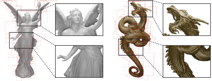
Figure 1. Adaptive coordinate networks for neural scene representation (acorn), can fit signals such as three-dimensional occupancy fields with high accuracy. Here we demonstrate fitting a 3D occupancy field where inputs to the model are continuous coordinates in space, and outputs are the occupancy at those positions. acorn optimizes a partition of space while training by allocating more blocks to regions with fine details. Shown here are two detailed 3D scenes obtained with our architecture, Lucy from the Stanford 3D Scanning Repository and a detailed model of a dragon as well as their optimized decompositions at the end of training.

1. Introduction

How we represent signals has a tremendous impact on how we solve problems in graphics, computer vision, and beyond. Traditional graphics representations, such as meshes, point clouds, or volumes, are well established as robust and general-purpose tools in a plethora of applications ranging from visual effects and computer games to architecture, computer-aided design, and 3D computer vision. Traditional representations, however, are not necessarily well-suited for emerging applications in neural rendering, imaging, geometric modeling, and simulation. For these emerging applications, we require representations that are end-to-end differentiable, quickly optimizable, and scalable in learning-based pipelines. Traditional representations are often at odds with these properties since they scale according to Nyquist sampling requirements and require storing spatio-temporal samples explicitly in memory.

A variety of neural scene representations have been proposed over the last few years, which overcome some of these limitations (see Sec. 2 for a detailed discussion). Among these, explicit neural representations usually focus on mimicking the functionality of traditional discrete representations in a differentiable manner, often using discrete grids of learned features. Implicit representations, or coordinate networks, parameterize images, shapes, or other signals using neural networks that take a spatio-temporal coordinate as input and output a quantity of interest, such as color, volume density, or a general feature. Coordinate networks are continuous, and the complexity of the signals they represent is limited by the capacity of the representation network rather than the grid size of an explicit representation.

While emerging neural scene representations are promising building blocks for a variety of applications, one of the fundamental challenges of these representations is their inability to scale to complex scenes. For example, although explicit representations are fast to evaluate, their memory requirements often scale unfavorably since they require storing a large number of explicit features. Coordinate networks can be more memory efficient, because they do not necessarily need to store features on a grid, but they are computationally inefficient; for every coordinate that is evaluated (e.g., every pixel of an image or every point in a 3D space), an entire feedforward pass through the underlying representation network has to be computed. Therefore, existing neural representations are either computationally inefficient or memory intensive, which prevents them from scaling to large-scale or complex scenes.

Here, we propose a new hybrid implicit–explicit coordinate network architecture for neural signal representations. Our architecture automatically subdivides the domain of the signal into blocks that are organized in a multiscale fashion. The signal is modeled by a coordinate network that takes a multiscale block coordinate as input and outputs a quantity of interest continuously within the block. Unlike existing local implicit representations (Peng et al., 2020; Chabra et al., 2020; Jiang et al., 2020b; Chen et al., 2021; Kellnhofer et al., 2021), our architecture does not map the input coordinate directly to the output, but to an intermediate low-resolution grid of local features using a coordinate encoder. Using a separate but small feature decoder, these features can be efficiently interpolated and decoded to evaluate the representation at any continuous coordinate within the block. The benefit of this two-stage approach is that the bulk of the computation (generating feature grids) is performed only once per block by the coordinate encoder, and querying points within the block requires minimal computational overhead using the feature decoder. This design choice makes our representation much faster to evaluate and more memory efficient than existing explicit, coordinate-based, or hybrid solutions.

	Comp. Eff.	Mem. Eff.	Multiscale	Pruning
Explicit	✓	✗	✗	✗
Global Implicit	✗	✓	✗	✗
Local Implicit	✓or ✗	✗ or ✓	✗	✗
NSVF	✓or ✗	✗ or ✓	✗	✓
Ours	✓	✓	✓	✓

Table 1. Existing explicit representations are memory inefficient and implicit coordinate networks are computationally inefficient, as they require a full forward pass for each coordinate they evaluate. Local implicit approaches and neural sparse voxel fields (NSVF) (Liu et al., 2020a) make a direct tradeoff between memory and computational efficiency, as they require an additional volume with latent codes or features to be stored. Our multiscale representation is computational and memory efficient, it allows us to prune empty space in an optimized manner, and we demonstrate its application to large-scale image and complex 3D shape representation.

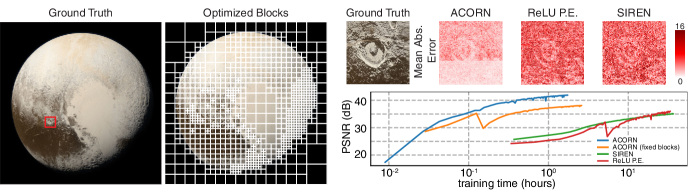
Figure 2. Large-scale image fitting. We fit networks to a 64 MP image of the dwarf planet Pluto, captured by the New Horizons space probe. The optimized block decomposition for our method is shown along with error maps for an inset of the image for our method, as well as a ReLU P.E. network (Mildenhall et al., 2020) and a SIREN (Sitzmann et al., 2020). All networks use roughly 9.5 M parameters. A plot of image PSNR vs. training time for all networks (including ours with a fixed, uniform block decomposition) is shown from 1,000 to 100,000 iterations. Our multiscale representation network converges to a PSNR of ¿40 dB in about one hour, whereas other representations struggle to adequately fit this image in more than one day.

Moreover, we propose a novel training strategy that adaptively refines the scale and locations of the block coordinates during training. The resulting block decomposition is similar in spirit to a quadtree or an octree (Fig. 2, center left). Determining the optimal block decomposition is a resource allocation problem that involves solving an integer linear program periodically during training. Notably, optimizing the block partitioning does not require pre-processing of the input signal and runs online using the training loss within each block. Effectively, this approach prunes empty space and allocates the capacity of the representation network in an optimal multiscale fashion. We also note that a single network is shared across all blocks of a scene, regardless of position or scale.

The design choices discussed above make our representation both computationally efficient (i.e., by pruning empty space, a hierarchical subdivision, and using block-wise coordinate networks) and memory efficient (i.e., by the hybrid implicit–explicit network design). Our representation trains significantly faster than other coordinate networks and it does not spend resources on redundant parts of the signal. The inference time varies over the scene and depends on its local complexity. These benefits allow us to demonstrate the first experiments that fit gigapixel images as well as complex 3D scenes with a neural scene representation. For example, the largest image we processed (see Sec. 4) has a resolution of 51,200 $\times$ 19,456 pixels, which is about 1,000$\times$ larger than what has been demonstrated to date, and our approach is able to fit this image at a quality of nearly 40 dB peak signal-to-noise ratio (PSNR) within just a few hours. Similarly, we demonstrate that our approach is able to represent 3D shapes significantly faster and better than existing neural scene representations.

Our approach is a core building block of emerging neural approaches to imaging, geometric modeling, rendering, and simulation. We expect it to be of fundamental importance to many different areas in computer graphics and interactive techniques. Source code is publicly available.

Specifically, our contributions include

• a new multi-scale hybrid implicit–explicit signal representation network architecture,

• a training strategy that integrates an integer linear program for automatic multiscale resource allocation and pruning,

• state-of-the-art results for representing large-scale images and complex 3D scenes using neural representations.

2. Related Work

A large body of work has been published in the area of neural scene representation. This section provides a best attempt to concisely overview this emerging research area.

Neural Scene Representations

Among the recently proposed neural scene representations, explicit representations directly represent 2D or 3D scenes using imperfect meshes (Hedman et al., 2018; Thies et al., 2019; Riegler and Koltun, 2020; Zhang et al., 2021), multi-plane (Zhou et al., 2018; Mildenhall et al., 2019; Flynn et al., 2019) or multi-sphere (Broxton et al., 2020; Attal et al., 2020) images, or using a voxel grid of features (Sitzmann et al., 2019a; Lombardi et al., 2019). The primary benefit of explicit representations is that they can be quickly evaluated at any position and can thus be rendered fast. However, explicit grid-based representations typically come with a cost of large memory requirements and are thus challenging to scale.

Alternatively, coordinate networks implicitly define a 2D or 3D scene using neural networks. Many variants of these networks have been proposed in the last few years for modeling 3D shapes (Atzmon and Lipman, 2020; Chabra et al., 2020; Chen and Zhang, 2019; Davies et al., 2020; Genova et al., 2020; Gropp et al., 2020; Park et al., 2019; Mescheder et al., 2019; Michalkiewicz et al., 2019; Sitzmann et al., 2020), view synthesis (Chan et al., 2021; Eslami et al., 2018; Mildenhall et al., 2020; Niemeyer et al., 2020a; Jiang et al., 2020a; Henzler et al., 2019; Nguyen-Phuoc et al., 2020; Schwarz et al., 2020; Sitzmann et al., 2019b; Yariv et al., 2020; Liu et al., 2020b), semantic labeling (Kohli et al., 2020), and texture synthesis (Oechsle et al., 2019; Saito et al., 2019). The shared characteristic of all of these approaches is that signals or scenes are implicitly defined by a network that can be queried for continuous coordinates, rather than on a discrete pixel or voxel grid. This implies that the complexity of the scene is limited by the capacity of the network rather than the resolution of a grid. To represent a reasonably complex scene, however, coordinate networks must be fairly large, which makes them slow to query because an entire feedforward pass through the network needs to be computed for evaluating every single coordinate. This limitation makes current implicit representations difficult to scale.

The closest existing approaches to ours are local implicit methods. With applications to fitting shapes (Peng et al., 2020; Chabra et al., 2020; Jiang et al., 2020b) or images (Chen et al., 2021), they use implicit networks to predict local or part-level scene information. In these models, a single globally shared decoder network operates on local coordinates within some explicit grid representation. Each grid cell needs to store a latent code or feature vector that the local network is conditioned with. These methods largely differ in how this latent code vector is estimated, either through iterative optimization (Chabra et al., 2020; Jiang et al., 2020b) or directly by a convolutional encoder network operating on a point cloud (Peng et al., 2020). In all cases, additional information, such as the volume of latent code vectors or the input point cloud, have to be stored along with the implicit network, which makes these methods less memory efficient and less scalable than a fully implicit representation that requires coordinate inputs alone. Similar to our approach, neural sparse voxel fields (NSVF) (Liu et al., 2020a) prunes empty space so that the representation network does not have to be evaluated in these regions. NSVF uses a heuristic coarse-to-fine sampling strategy to determine which regions are empty but, similar to local implicit models, requires storing an explicit volume of features representing the scene at a single scale.

As outlined by Table 1, our network architecture is different from these approaches in several important ways. First, our method is the only multiscale representation. This allows us to use the network capacity more efficiently and also to prune empty space in an optimized multiscale fashion. Second, we realize that the computational bottleneck of all implicit networks is the requirement to compute many forward passes through the networks, one per coordinate that is evaluated. This is also true for local implicit approaches. Instead, our architecture efficiently evaluates coordinates at the block level. Third, our architecture is a “pure” coordinate network in that it does not require any additional features as input, so it is more memory efficient than approaches that store an explicit grid of features or latent codes.

Neural Graphics

Neural rendering describes end-to-end differentiable approaches for projecting a 3D neural scene representation into one or multiple 2D images. Inverse approaches that aim at recovering a scene representation from 2D images require this capability to backpropagate the error of an image rendered from some representation with respect to a reference all the way into the representation to optimize it. Each type of representation may require a unique rendering approach that is most appropriate. For example, implicitly defined signed distance functions (SDFs) use ray marching or sphere tracing–based neural rendering (e.g., (Sitzmann et al., 2019b; Jiang et al., 2020a; Liu et al., 2020b; Yariv et al., 2020)) whereas neural volume representations use a differentiable form of volume rendering (e.g., (Sitzmann et al., 2019a; Lombardi et al., 2019; Mildenhall et al., 2020; Liu et al., 2020a; Niemeyer et al., 2020b)). A more detailed overview of recent approaches to neural rendering can be found in the survey by Tewari et al. (2020). Similarly, neural representations and methods have recently been proposed for simulation problems (Kim et al., 2019; Li et al., 2020; Sitzmann et al., 2020).

The multiscale neural representation we propose is agnostic to the type of signal it represents and we demonstrate that it applies to different signal types, including 2D images and 3D shapes represented as occupancy networks (Mescheder et al., 2019). Thus, our representation is complementary to and, in principle, compatible with most existing neural rendering and graphics approaches. Yet, a detailed exploration of all of these applications is beyond the scope of this paper.

Multiscale Signal Representations

Our multiscale network architecture is inspired by several common techniques used in other domains of graphics and interactive techniques, including adaptive mesh refinement used for fluid solvers or solving other partial differential equations (e.g., (Berger and Oliger, 1984; Huang and Russell, 2010)), bounding volume hierarchies used for collision detection or raytracing, and multiscale decompositions, such as wavelet transforms, that represent discrete signals efficiently at different scales.

3. Multiscale Coordinate Networks

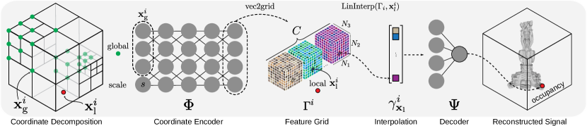
Figure 3. Illustration of multiscale network architecture for 3D shape representation, including the adaptive coordinate decomposition, the larger coordinate encoder network, the discrete feature grid, feature interpolation, the smaller decoder network, and the reconstructed signal.

Our approach for multiscale representation networks relies on two main components: (1) a multiscale block parameterization that partitions the input space according to the local signal complexity, and (2) a network architecture consisting of a coordinate encoder and a feature decoder that efficiently map input spatial and scale coordinates to an output value.

3.1. Multiscale Block Parameterization

At the core of our multiscale block parameterization is a tree-based partition of the input domain. Specifically, we partition the domain with a quadtree in two dimensions or an octree in three dimensions, and we fix the finest scale, or maximum depth, of the tree (see Figure 3). As opposed to traditional multiscale decompositions, where each value of the input domain is represented at multiple scales (e.g., each pixel in an image pyramid), our approach partitions space such that each input value is represented at a single scale. That is, while a particular input domain value may fall within the bounds of potentially multiple quadrants or octants (hereafter blocks) at different scales, we associate each value with one “active” block, $B_{i}$, at a single scale. The input domain is thus partitioned into a set of active blocks, $\mathcal{B}$, that together cover the domain. In summary, the “active blocks” are the currently selected blocks in the octree/quadtree that uniquely represent a region of the input space. The selection of active blocks is part of an optimization problem we describe in Section 3.3.

The blocks and input domain values within each block are addressed by a global block index and a continuous local coordinate. The global block index, $\mathbf{x}_{\text{g}}^{i}\in\mathbb{R}^{d_{\text{in}}+1}$, gives the global coordinate of $B_{i}$. We define $d_{\text{in}}$ as the dimensionality of the input coordinate domain and the last element of $\mathbf{x}_{\text{g}}^{i}$ encodes the normalized scale of the block corresponding to its discrete level in the quadtree or octree.

We also introduce a continuous local coordinate $\mathbf{x}_{\text{l}}^{i}$ to parameterize the input domain within $B_{i}$. Here, $\mathbf{x}_{\text{l}}^{i}$ is a $d_{\text{in}}$-dimensional vector whose elements take on values between -1 and 1, or $\mathbf{x}_{\text{l}}\in\mathbb{R}^{d_{\text{in}}}_{[-1,1]}=\{(x_{1},\ldots,x_{d_{\text{in}}})^{T}\ |-1\leq x_{i}\leq 1\}$. Thus any continuous coordinate $\mathbf{x}$ in the input domain can be described by pairing the global block index, $\mathbf{x}_{\text{g}}^{i}$, of its containing block with the continuous local coordinate, $\mathbf{x}_{\text{l}}^{i}$, which describes a relative position within the block.

3.2. Neural Network Architecture

The representation network (see Figure 3) contains a coordinate encoder

(1) $$\Phi:\mathbb{R}^{d_{\text{in}}+1}\rightarrow\mathbb{R}^{C\times N_{1}\times\cdots\times N^{d_{\text{in}}}},\quad\mathbf{x}_{\text{g}}^{i}\mapsto\Phi(\mathbf{x}_{\text{g}}^{i})=\Gamma^{i},$$

which maps a global block index to a grid of features $\Gamma^{i}$ of dimension $N_{1}\times\cdots N_{d_{\text{in}}}$ (i.e., it has size $N_{i}$ along the $i$-th dimension) with $C$ feature channels (i.e., each cell in $\Gamma^{i}$ is a vector of dimension $C$). Both the $N_{i}$’s and $C$ are hyperparameters. Given a continuous local coordinate $\mathbf{x}_{\text{l}}$, a feature vector is extracted as

(2) $$\textsc{LinInterp}\left(\Gamma^{i},\mathbf{x}_{\text{l}}^{i}\right)=\gamma^{i}_{\mathbf{x}_{\text{l}}}\in\mathbb{R}^{C},$$

where LinInterp is the multivariate linear interpolation (e.g., bilinear when $d_{\text{in}}=2$ or trilinear when $d_{\text{in}}=3$) of the feature grid and is used to calculate a feature $\gamma^{i}_{\mathbf{x}_{\text{l}}}$ at any relative coordinate $\mathbf{x}_{\text{l}}^{i}$ within the grid. A feature decoder $\Psi$ maps the feature vector to the output, $\mathbb{y}^{i}$, as

(3) $$\Psi:\mathbb{R}^{C}\rightarrow\mathbb{R},\quad\gamma_{\mathbf{x}_{\text{l}}}^{i}\mapsto\Psi(\gamma_{\mathbf{x}_{\text{l}}}^{i})=\mathbb{y}^{i}\approx\mathbb{y}_{\text{GT}}^{i}.$$

Here, the output of the decoder approximates the signal of interest $\mathbb{y}_{\text{GT}}$ at the global coordinate $\mathbf{x}$.

In practice, we implement both networks using multi-layer perceptrons (MLP) with ReLU nonlinearities. We apply a positional encoding (Mildenhall et al., 2020) to the global block indices before input to the coordinate encoder, and the feature decoder consists of a small MLP with a single hidden layer that is efficient to evaluate.

One key advantage of this two-stage architecture is that it greatly reduces the computational expense of evaluating many coordinates within the same block. While the coordinate encoder $\Phi$ contains the bulk of the network parameters and is the most expensive component to evaluate, only a single forward pass is required. Once the feature grid is generated, all local coordinates within the block can be evaluated using a lightweight interpolation operation and a forward pass through the small decoder network. During training time, this also reduces memory requirements as we are only required to store intermediate activations of the larger coordinate encoder network (used for backpropagation) for a small number of block indices rather than every single input coordinate. Another advantage is a potential improvement in network capacity since feature grids can be re-used for signals with repetitive structures across spatial locations and scales.

3.3. Online Multiscale Decomposition

One challenge in training neural representations efficiently is that most training samples should come from regions of the signal of interest that have the greatest complexity or are most challenging to learn. Likewise, at inference time, most of the computation should be devoted to accurately generating complex regions of the signal rather than simple regions. For example, for an image, we expect that it is possible to learn and infer flat-textured regions more efficiently than highly textured regions while yet achieving the same image quality. These observations are at odds with conventional neural representations which use an equal density of training samples for all regions of an image or 3D surface and require an equal number of forward passes through the network to render each region of the representation.

Here, we propose a new automatic decomposition method that allocates network resources adaptively to fit a signal of interest. Our technique is inspired by adaptive mesh refinement methods in simulation techniques and finite-element solvers which refine or coarsen meshes at optimization time to improve solution accuracy while minimizing computational overhead (Berger and Oliger, 1984).

During training time, we fix the maximum number of active blocks in the decomposition, allocate $N_{1}\times\cdots\times N_{d_{\text{in}}}$ training samples to each block, and track the average signal fitting loss within each block. The maximum number of blocks is a hyperparameter that can be tuned according to the computational budget and network capacity. At frequent intervals during training, we apply a non-differentiable update to the scale of each block by solving a resource allocation problem that seeks to minimize the fitting loss while maintaining fewer blocks than the prescribed maximum.

Solving the resource allocation problem causes blocks to merge or combine, resulting in an update to the set of active blocks or global block indices used during training. Since the number of training samples within each block is fixed, the procedure dynamically allocates more samples to harder-to-fit regions by placing finer blocks at the corresponding locations. At inference time, coarse blocks are used to represent less detailed regions such that the signal can be generated with fewer forward passes through the more expensive coordinate encoder and more passes through the lightweight feature decoder.

Online optimization details.

We formulate the resource allocation problem as an Integer Linear Problem (ILP) where each active block $B_{i}$ in the partition $\mathcal{B}$ is considered in the context of its sibling blocks. In a quadtree, each node has four children, thus each block, $B_{i}$ has a set of three siblings, $\mathcal{S}(i)$, and sibling groups are composed of $N_{S}=4$ blocks. Likewise, blocks in an octree have seven siblings with $N_{S}=8$ blocks in a sibling group. Thus, for any active block we can use three binary decision variables to encode whether it merges with its siblings to a coarser scale ($I^{\uparrow}$), stays as is ($I^{=}$), or splits to create a new group of siblings (children) at a finer scale ($I^{\downarrow}$):

(4) $$\mathbb{I_{i}}=\left(I^{\uparrow}_{i},I^{=}_{i},I^{\downarrow}_{i}\right)^{\intercal}\in\{0,1\}^{3}.$$

To merge a block, all siblings must be active (i.e., members of the current partition $\mathcal{B}$) at the same scale and have $I^{\uparrow}=1$. We define a corresponding “grouping” indicator as

(5) $$I^{g}_{i}\overset{\text{def.}}{=}\frac{1}{N_{S}}\left(I^{\uparrow}_{i}+\sum_{j\in\mathcal{S}(i)}I^{\uparrow}_{j}\right),$$

which evaluates to $1$ when all siblings are set to merge.

The decisions for a block to merge, split or stay at the same scale are mutually exclusive, which we encode in the constraint

(6) $$I^{g}_{i}+I^{\downarrow}_{i}+I^{=}_{i}=1.$$

The partition obtained from the optimization must not contain more than $N_{B}$ blocks. If a block splits ($I^{\downarrow}_{i}=1$) it contributes $N_{S}$ blocks to the new partition, or if it merges ($I^{\uparrow}_{i}=1$) it contributes $\frac{1}{N_{S}}$ blocks. Thus, we can constrain the total number of blocks in the optimized partition as

(7) $$\left(\sum_{i}\frac{1}{N_{S}}\,I^{\uparrow}_{i}+I^{=}_{i}+N_{S}\,I^{\downarrow}_{i}\right)\leq N_{B}.$$

Ultimately we wish to optimize the block partition such that the new partitioning has a lower fitting error to the signal of interest after it is optimized. Thus, for each block, we require an estimate of the fitting error incurred from a decision to merge, stay the same, or split. We arrange these estimates into a vector of weights $\mathbb{w}_{i}=\left(w_{i}^{\uparrow},w_{i}^{=},w_{i}^{\downarrow}\right)^{\intercal}$ and solve the following optimization problem to find the new partition.

(8) minimize $$\sum_{i}\mathbb{w}_{i}^{\intercal}\,\mathbb{I}_{i}$$

subject to $$\begin{cases}\eqref{eq:cstr_choice}\>\forall B_{i}\in\mathcal{B},\\ \eqref{eq:cstr_knapsack}.\end{cases}$$

To calculate the values of $\mathbb{w}_{i}$, we first compute the mean block error $E^{i}$ using an application dependent loss $\ell:\mathbb{R}^{d_{\text{out}}}\times\mathbb{R}^{d_{\text{out}}}\mapsto\mathbb{R}$ taken over the output of the feature decoder $\mathbb{y}^{i}$ for all the corresponding continuous local coordinates $\mathbf{x}_{\text{l}}^{i}$.

(9) $$E^{i}=\mathbb{E}_{\mathbf{x}_{\text{l}}}\left[\ell\left(\mathbb{y}^{i},\mathbb{y}_{\text{GT}}\left(\mathbf{x}\right)\right)\right].$$

where $\mathbb{E}_{\mathbf{x}_{\text{l}}}[\cdot]$ denotes the expectation (empirical mean) taken over the $N_{l}$ sampled fine coordinates $\mathbf{x}_{\text{l}}$ (see Alg. 1). Then, we calculate $w_{i}^{=}$ for each block with volume $\text{Vol}_{i}$ as

(10) $$w_{i}^{=}=\text{Vol}_{i}\cdot E^{i},$$

Here, weighing the mean block loss by the volume is important for a consistent error estimate across scales. The error for merging ($w_{i}^{\uparrow}$) is estimated as the error of the parent block, $\mathcal{P}(i)$, when an estimate of its error is available (that is, if the parent has been fitted in the past). Otherwise we approximate the error with $N_{S}$ times the current error.

(11) $$w_{i}^{\uparrow}=\begin{cases}\frac{1}{N_{S}}\,w_{\mathcal{P}(i)}^{=},&\text{if parent's error is available},\\ (N_{S}+\alpha)\,w_{i}^{=}&\text{otherwise}.\end{cases}$$

Using $\alpha>0$ captures the assumption that the error when merging blocks is worse than $N_{S}$ times the current block error.

The error for splitting a block ($w_{i}^{\downarrow}$) is similarly estimated as the sum of the errors of the children blocks when those estimates are available. Otherwise, we use an approximate estimate of $\frac{1}{N_{S}}$ times the current error.

(12) $$w_{i}^{\downarrow}=\begin{cases}\sum_{j\in\mathcal{C}(i)}w_{j}^{=},&\text{if children's errors available},\\ (\frac{1}{N_{S}}-\beta)\,w_{i}^{=}&\text{otherwise}.\end{cases}$$

with $\mathcal{C}(i)$ the children of $i$. Here, using $\beta>0$ assumes that the error when splitting a block is likely to be better than $\frac{1}{N_{S}}$ times the current error.

Parameters : 

$T$: max number of iterations

$T_{\text{optim.}}$: number of iter. between each partition optimization

$T_{\text{pruning}}$: number of iter. between each partition pruning

$t\leftarrow 0$

repeat

       foreach block $B^{i}\in\mathcal{B}$ with global coord. $\mathbf{x}_{\text{g}}^{i}$ do

             Compute the feature grid $\Gamma^{i}=\Phi(\mathbf{x}_{\text{g}}^{i})$

             Stratified sample $N_{l}$ local coord. $\mathbf{x}_{\text{l}}^{i,j}\sim[-1,1]^{d_{\text{in}}},\forall j<N_{l}$

             foreach local coord. $\mathbf{x}_{\text{l}}^{i,j}$ do

                   Calculate feature by interp. $\gamma^{i,j}_{\mathbf{x}_{\text{l}}}=\textsc{LinInterp}\left(\Gamma_{i},\mathbf{x}_{\text{l}}^{i,j}\right)$

                   Decode the feature $\mathbb{y}^{i,j}=\Psi(\gamma^{i,j}_{\mathbf{x}_{\text{l}}})$

                  

             end foreach

            

            Compute block error $E^{i}=\mathbb{E}_{\mathbf{x}_{\text{l}}}[\ell(\mathbb{y}^{i,j},\mathbb{y}^{i,j}_{\text{GT}})]$

             Update ILP weights $\{w_{i}^{\uparrow},w_{i}^{=},w_{i}^{\downarrow}\}$ from $E^{i}$

            

       end foreach

      Compute loss $\mathcal{L}=\frac{1}{|\mathcal{B}|}\sum_{B^{i}\in\mathcal{B}}E^{i}$

       Backpropagate $\mathcal{L}$ to update $\Phi$ and $\Psi$

       if  $t\mod T_{\text{optim.}}=0$ then

             Optimize the partition $\mathcal{B}$

       end if

      if  $t\mod T_{\text{pruning}}=0$ then

             Prune the partition $\mathcal{B}$

            

       end if

      $t\leftarrow t+1$

until $t\geq T$

ALGORITHM 1 Adaptive Multiscale Network Training

Solving the ILP

We solve the ILPs to optimality with a branch-and-bound algorithm using the solver implemented in the Gurobi Optimization Package (2021). The solver is fast: using a thousand active blocks takes less than $100$ ms which is negligible with respect to the training time of the networks since the optimization only occurs every few hundred training steps.

Interpretation

The ILP selects blocks to split and merge based on the feedback of the error fitting signal. The linear constraint in Equation (8) and the design of our weights Eq. (10), (11), (12) act in a way that is intuitively similar to sorting the blocks based on the fitting error and splitting or merging blocks with the highest or lowest error. However, compared to such an approach, solving the ILP offers a few advantages. The main advantage of this formulation is that it allows us to only specify the maximum number of blocks in the partition, which we assumed correlates to the maximum capacity of our encoder. Besides, it avoids other heuristics such as specifying the number of blocks that can merge/split each iteration.

3.4. Pruning

As the partition gets optimized over the course of training, it happens that certain blocks represent regions that are perfectly uniform. Those regions can be described by a single value, for instance, the color of a constant area in an image, or zero for the empty space in an occupancy field. To avoid learning the same value for a whole region in the multiscale network, we prune the block from the partition. It cannot be further split and its value is set in a look-up table. Since the block is no longer active, it frees up space in the partition by loosening the constraint in Equation (8). Thus, the next time the ILP is solved, it can further split active blocks. This will result in a finer partition. To decide whether to prune a block $B_{i}$ we found that meeting both the following criteria worked very well in practice:

Low error:

we check that the fitting error $E_{i}$ of the block $B_{i}$ is less than an application specific threshold (depending on the choice of $\ell(\cdot,\cdot)$).

Low variance in the block:

we make sure that the values output by the network $\{\Psi(\mathbf{x}_{\text{l}}^{i,j})\}_{j}$ in the block are not spread.

We show results of pruning in a following section on representing 3D scenes.

4. Representing Gigapixel Images

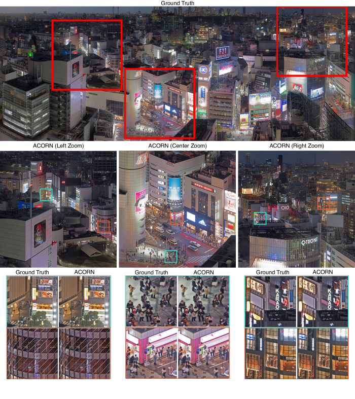
Figure 4. Gigapixel-scale image fitting. We show the results of fitting a Gigapixel panorama photo of Tokyo using the proposed multiscale architecture, achieving a PSNR of 38.59. Top row; ground truth input. Middle row; 10K $\times$ 10K zoom-ins of multiscale result. Bottom row; 1K $\times$ 1K zoom-ins of ground truth and multiscale result. (Photo: Trevor Dobson, https://creativecommons.org/licenses/by-nc-nd/2.0/)

In this section, we discuss the large-scale image representation experiments we show in Figures 2 and 4. Note that previous neural image representations (e.g., (Sitzmann et al., 2020; Chen et al., 2021)) have been limited to images with resolutions of up to a megapixel (MP). With resolutions of 64 MP and $\sim$1 GP, respectively, our experiments far exceed these limits.

Table 2. Quantitative image fitting results.

	Train Time	GPU Mem.	Model Param.	PSNR (dB) $\uparrow$	SSIM $\uparrow$
Pluto Image (64 MP)
ReLU P.E.	33.9 h	13.3 GB	9.5 M	35.99	0.93
SIREN	37.0 h	20.9 GB	9.5 M	35.08	0.92
ACORN (fixed)	2.6 h	2.4 GB	9.5 M	38.08	0.95
ACORN	1.8 h	2.4 GB	9.5 M	41.90	0.97
Tokyo Image (996 MP)
ACORN	36.9 h	33.0 GB	168.0 M	38.59	0.94

4.1. Image Fitting Task

To fit an image with ACORN, we train in an online fashion where we generate $N_{l}$ random stratified samples within active block of the multiscale decomposition. Then, the values of $\mathbb{y}_{\text{GT}}$ are determined by bilinear interpolation of the corresponding global coordinates on the target image. The training proceeds according to Alg. 1, though we disable the pruning step since we assume all blocks contain some non-zero texture. We use a mean-squared error loss between the network output and the target image for each block as

(13) $$\ell(\mathbb{y}^{i},\mathbb{y}^{i}_{\text{GT}})=\lVert\mathbb{y}^{i}-\mathbb{y}^{i}_{\text{GT}}\rVert_{2}^{2}.$$

During training, we optimize the block partition every 500 iterations and fix the maximum number of blocks to $N_{B}=1024$.

Baselines.

We compare our method to state-of-the-art coordinate representation networks designed for fitting images: sinusoidal representation networks (SIREN), and an MLP using ReLU non-linearities and a frequency-based positional encoding strategy (Mildenhall et al., 2020; Tancik et al., 2020). We also add an additional ablation study that disables the multiscale block optimization and instead uses a fixed decomposition by evenly distributing the $N_{B}$ blocks at a single scale across the domain. To compare the methods we set the parameter counts of the corresponding networks to be approximately equal. More details about the optimization and network architectures are provided in Appendix A.

4.2. Performance

We demonstrate the performance of ACORN by fitting two large-scale images. The first is an image of Pluto (shown in Figure 2), captured by the New Horizons space probe. The image has a resolution of 8,192 $\times$ 8,192 pixel (64 MP) and has features at varying scales, making it ideal for a multiscale representation. The adaptive grid optimized by our resource allocation strategy clearly shows that the representation uses significantly smaller blocks to represent fine details, such as the craters, whereas the empty and large uniform areas are represented at much coarser scales. As seen in the convergence plots, our representation converges about two orders of magnitude faster compared to state of the art coordinate networks and it fits this challenging image at a significantly higher quality well above 40 dB PSNR (see Table 2 and color-coded error maps in Figure 2). All baselines are evaluated on the same an NVIDIA RTX 6000 GPU, and metrics are reported after 100,000 iterations of training.

In addition to fitting this image faster and better than alternative network architectures, our model only requires 2.4 GB of memory whereas ReLU with positional encoding (P.E.) (Mildenhall et al., 2020) and SIREN (Sitzmann et al., 2020) require 13.3 GB and 20.9 GB, respectively. Note that while the parameter counts of the methods are similar, our approach uses far less memory because of the two-stage inference technique. For backpropagation, intermediate activations through the coordinate encoder are stored only once per block while intermediate activations for the feature decoder (with far fewer parameters) are stored for each local coordinate.

Table 3. Comparison of ACORN models fitted on the Pluto image ($1024\times 1024$) varying the number of blocks used in the quadtree decomposition (training time reported using a NVIDIA Titan V).

Number of blocks	64	256	1024	4096
PSNR at convergence (dB)	31.4	37.3	40.1	37.7
Training time to 50 K it. (min)	45	63	140	388
Training time to 30 dB PSNR (min)	7	4	10	48

We also note the improved performance of our technique relative to using the same network architecture, but with a fixed block decomposition. While fixing the block decomposition yet results in rapid convergence and a network that outperforms other methods (see Figure 2 and Table 2), we find that including the block decomposition significantly improves image quality. We also notice slightly faster training times using the adaptive block decomposition because we start the training with only 64 blocks at a coarse scale, leading to faster iterations at the beginning of training.

The gigapixel image of Tokyo shown in Figure 4 has a resolution of 19,456 $\times$ 51,200 pixels, which is about three orders of magnitude higher than what recent neural image representations have shown. Again, this image captures details over the entire image at different scales. The multiscale architecture is the same as the one used to fit the Pluto result in Figure 2, though we increase the parameter count as described in Table 2 and Appendix A. A visualization of the optimized grid showing the block decomposition and additional training details are included in the supplement.

As we have shown, ACORNs can be scaled to flexibly represent large-scale 2D images, offering significant improvements to training speed, performance, and the overall practicality of this task.

4.3. Interplay between the quadtree decomposition, time and fitting accuracy

We perform an experiment that varies the number of blocks used in the fitting of the Pluto image (Figure 2) downsampled at a resolution of $1024\times 1024$. Results are summarized in Table 3. With fewer blocks, the image is represented at a coarser level of the octree: training is faster since there are fewer blocks to fit but the overall model accuracy is lower. Increasing the number of blocks improves accuracy until the coordinate encoder saturates and fails to generate accurate features across the entire image at the finest level of the octree.

5. Representing Complex 3D Scenes

Table 4. Quantitative 3D fitting results (Thai Statue).

	Train Time	GPU Mem.		Model Param.
SPSR	0.128 h	N/A		N/A
Conv. Occ.	100 h	9.1 GB		4.167 M
SIREN	29.28 h	14.3 GB		16.8 M
ACORN	4.25 h	1.7 GB		17.0 M
	IoU ($\uparrow$)	Chamfer-$L_{1}$ ($\downarrow$)	Precision ($\uparrow$)	Recall ($\uparrow$)	F-Score ($\uparrow$)
SPSR	0.809	4.76e-04	0.891	0.897	0.894
Conv. Occ.	0.965	2.16e-05	0.972	0.992	0.982
SIREN	0.992	2.06e-05	0.996	0.996	0.996
ACORN	0.999	1.55e-05	0.999	0.999	0.999

Table 5. Quantitative 3D fitting results (Engine).

	Train Time	GPU Mem.		Model Param.
SPSR	0.114 h	N/A		N/A
Conv. Occ.	108 h	9.1 GB		4.167 M
SIREN	29.21 h	14.3 GB		16.8 M
ACORN	7.77 h	1.7 GB		17.0 M
	IoU ($\uparrow$)	Chamfer-$L_{1}$ ($\downarrow$)	Precision ($\uparrow$)	Recall ($\uparrow$)	F-Score ($\uparrow$)
SPSR	0.843	1.19e-04	0.906	0.924	0.951
Conv. Occ.	0.840	7.93e-04	0.877	0.952	0.913
SIREN	0.961	1.09e-04	0.980	0.980	0.980
ACORN	0.987	8.46e-05	0.992	0.994	0.993

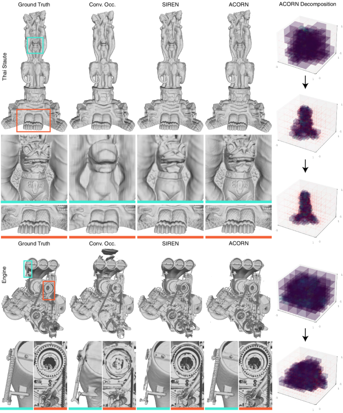
Figure 5. Complex 3D scene fitting. We compare the results of fitting highly detailed meshes of a Thai statue and an engine using the baseline methods and our proposed multiscale architecture. ACORN is able to capture both global and local geometric features better than all other baselines. The evolution of the learned block decompositions during training are shown on the right. (Engine Model: ChrisKuhn, https://creativecommons.org/licenses/by/2.0/)

The benefits of a multiscale representation follow when moving from image representation to 3D scene representation. We benchmark our method against Screened Poisson Surface Reconstruction (SPSR) (Kazhdan and Hoppe, 2013), a classical method for obtaining watertight surfaces from point clouds, Convolutional Occupancy Networks (Peng et al., 2020), a recent example of local shape representations, and SIREN (Sitzmann et al., 2020), a state-of-the-art coordinate representation.

We compare representations on the task of representing the occupancy field of detailed 3D models. The Thai Statue, obtained from the Stanford 3D Scanning Repository (2014), consists of 10 million polygons and depicts an intricate resin statue. While the general shape is simple, fine details of the reliefs are challenging to capture with existing methods. The Dragster Engine, obtained free from BlendSwap, consists of 512 thousand polygons and is a recreation of an engine used in Top Fuel drag-racing. The thin features and hard edges that make up the engine are difficult to faithfully recreate.

5.1. Occupancy Prediction Task

We benchmark representations on the task of fitting the occupancy fields (Mescheder et al., 2019) of 3D models. At training time, we sample 3D points $\mathbb{x}\in\mathbb{R}^{3}$ with a 50/50 split – half of the points are sampled near the mesh surface, half of the points are sampled uniformly within the volume. Given the input points, we predict occupancy values. We apply binary cross-entropy loss between the occupancy prediction of our network, $\mathbb{y}\in\mathbb{R}$ and the true occupancy, $\mathbb{y}_{\text{GT}}$:

(14) $$\mathcal{\ell}(\mathbb{y},\mathbb{y}_{\text{GT}})=-[\mathbb{y}_{\text{GT}}\cdot\text{log}(\mathbb{y})+(1-\mathbb{y}_{\text{GT}})\cdot\text{log}(1-\mathbb{y})].$$

As in (Mescheder et al., 2019), we compute the ground truth occupancy of arbitrary points using the even–odd rule. In contrast to the deep-learning approaches, SPSR instead takes a point cloud with oriented normals as input.

5.2. Applying Multiscale Model to Occupancy Prediction

In moving from representing images in two dimensions to representing shapes in three dimensions, we replace the quadtree with an octree and predict a dense feature cube rather than a feature grid. As described above, our online multiscale decomposition approach samples coordinates per octant, which dynamically allocates samples towards hard-to-fit regions and improves the sample efficiency of training. Details about the network architecture can be found in Appendix A.

Empty Octant Pruning

The nature of our multiscale representation, which represents the scene at different scales, enables an additional optimization to further improve training time and performance. Periodically during training, we identify octants that are likely to be empty and “prune” them from the tree. In doing so, we eliminate sampling from regions of empty space while also freeing up octants and model capacity for more difficult and complex regions (see Figure 5).

5.3. Metrics

We evaluate the performance of all models by predicting a $1024^{3}$ cube of occupancy predictions. We compare against the ground-truth occupancy values with Intersection over Union (IoU), Precision, Recall, and F-Score. We additionally use marching cubes (Lorensen and Cline, 1987) to extract surfaces and evaluate mesh similarity with Chamfer distance. Quantitative results for these metrics, along with the model size, GPU memory required at training, and training time required to reach the reported results, are reported in Tables 4 and 5. All experiments are run on an RTX 6000 GPU.

5.4. Evaluating Performance

As shown in Figure 5, ACORN represents complex shapes with higher accuracy than previous methods. Qualitatively, it is more capable than previous implicit methods (Conv. Occ., SIREN) at representing fine details, such as intricate reliefs and tightly-coiled springs. Quantitatively, our approach outperforms all baselines on volume and mesh accuracy metrics.

When compared to previous neural representations, the improvements in computational efficiency become apparent. By sharing the computation among sampled points, our approach significantly reduces the memory and time costs associated with training and querying a model. When trained with the same number of parameters and at the same batch size, our multiscale representation requires nearly an order of magnitude less memory than a comparable MLP-based implicit representation, and yet outperforms it on representation accuracy metrics.

6. Compression

Memory usage presented in Tables 2, 4 and 5 corresponds to GPU memory needed to store and train ACORN. The size of the representation itself is much smaller: it is equal to the number of parameters multiplied by their encoding size (32-bits floats in all our experiments). In Table 6 we provide the size of the uncompressed ACORN models (i.e., no weight quantization nor pruning). For context we also provide the uncompressed sizes of the images and 3D models. The network representation wins by a large margin against the uncompressed models in most cases. Compression could be applied to the ACORN representions in different ways to gain further savings (e.g., using pruning and quantization (Han et al., 2016)).

Table 6. Size of ACORN models and of the uncompressed and compressed data used for fitting.

		Uncompressed	Compressed	ACORN
img.	Pluto (8192$\times$8192)	n/a	192 MB	38 MB
	Tokyo (19456$\times$51200)	2.8 GB	169 MB	670 MB
shapes	Lucy (14 M vert.)	1.2 GB	380 MB	68 MB
	Dragon (930 K vert.)	66 MB	27 MB	68 MB
	Thai Statue (5 M vert.)	424 MB	126 MB	68 MB
	Engine (308 K vert.)	16 MB	4.4 MB	68 MB

7. Discussion

In summary, we propose an adaptive multiscale neural scene representation that fits large-scale 2D and complex 3D scenes significantly faster and better than existing neural scene representations. These capabilities are enabled by a new hybrid implicit–explicit coordinate network architecture and a custom training routine that adapts the capacity of the network to the target scene in an optimized multiscale fashion.

Limitations

Currently, our method is limited in several ways. First, each block of our decomposition represents the scene at a single scale rather than multiple scales to preserve network capacity. The selected decomposition typically represents the coarsest scale at which a specific scene part can be represented adequately. Yet, it might be helpful to represent scenes at multiple scales simultaneously. For example, this would provide an option to evaluate signals faster at coarser resolutions, similar to recent work (Takikawa et al., 2021). Second, although the integer linear program we use to update the block partitioning integrates well with our training routine, it is non-differentiable. Exploring differentiable alternatives may further accelerate convergence and efficiency of our method. Third, updating the partitioning requires retraining on new blocks, so we see temporary increases in the fitting loss periodically during training. Again, a differentiable form of the resource allocation could alleviate these shortcomings. Fourth, the maximum number of blocks is fixed a priori rather than globally optimized, due to the formulation of the integer linear program. Finally, we note that the training method does not explicitly enforce continuity of the signal across blocks, though we train the representation on coordinates within the entirety of each block (including the boundary). In practice, we observe high-quality fitting near the boundaries, though some minor artifacts can occasionally be observed (see Fig. 6).

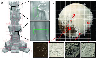
Figure 6. Demonstration of fitting at block borders. Though we do not explicitly enforce continuity across blocks, the borders between blocks yet retain high fitting quality. However, it is possible to observe small artifacts at the borders in the shape fitting (a) and image fitting (b) examples.

Future Work

In future work, we would like to address the aforementioned limitations. Moreover, we would like to explore additional applications in graphics and interactive techniques, such as neural rendering or fluid simulation. Source code is publicly available to foster application-domain-specific adjustments of our representation for any of these applications. Neural scene representations in general offer new ways to compress scenes, for example by quantizing or pruning the network after training, which would be interesting to explore in the future. We would also like to explore level-of-detail queries, e.g., for faster rendering at lower resolutions and explore representing higher-dimensional scenes, such as spatio-temporal data or graph based models.

8. Conclusion

Rapidly emerging techniques at the intersection of neural computing and computer graphics are a source of new capabilities in applications related to rendering, simulation, imaging, and geometric modeling. For these techniques, the underlying signal representations are crucial, but have been limited in many respects compared to traditional graphics representations. With our work, we take steps towards closing this gap by enabling large-scale images and complex shapes to be efficiently represented by neural networks.

Appendix A Implementation Details

A.1. Image Fitting

To fit the Pluto image we train our ACORN using a ReLU multi-layer perception (MLP) for the coordinate encoder and the feature decoder. The coordinate encoder is composed of 4 hidden layers with 512 hidden units each, and the final hidden layer outputs a feature grid with $C=16$ channels and width and height dimensions of $N_{1}=N_{2}=32$. We normalize the global block indices to fall within -1 and 1 and pass them through the positional encoding layer described by Mildenhall et al. (2020) with 6 frequencies. The feature decoder uses a single hidden layer with 64 hidden units. We set the maximum number of blocks to $N_{B}=1024$ and optimize for 100,000 iterations using the Adam optimizer (Kingma and Ba, 2014) and a learning rate of $1\times 10^{-3}$. The block partition is optimized every 500 iterations with $\alpha=0.2$ and $\beta=0.02$. For the baseline experiments with SIREN (Sitzmann et al., 2020) and ReLU P.E. (Mildenhall et al., 2020), we use MLPs with 4 hidden layers and 1536 hidden units to match the parameter count of the ACORN.

For the gigapixel image of Tokyo, we use the same architecture, but adjust the number of hidden units and layers. Here, we use $C=64$, $N_{1}=19$, and $N_{2}=50$. The coordinate encoder uses 10 positional encoding frequencies with 8 hidden layers, each with 2048 hidden units. Here, the block sizes are set to preserve the aspect ratio of the $19456\times 51200$ resolution image. The feature decoder is kept the same as previously described and the maximum number of blocks is $N_{B}=16384$. We optimize the image for 57,000 iterations, at which point the loss appeared to be converged.

A.2. 3D Occupancy Prediction

ACORN for 3D representations uses ReLU MLPs for the coordinate encoder and the feature decoder. The coordinate encoder is composed of 4 hidden layers with 512 hidden units each, and the final hidden layer outputs a feature cube of $C=18$ channels and width/height/depth dimensions of $N_{1}=N_{2}=N_{3}=12$. We normalize the global block indices to fall within -1 and 1 and pass them through the positional encoding layer described by Mildenhall et al. (2020) with 6 frequencies. The feature decoder uses a single hidden layer with 64 hidden units. We set the maximum number of octants to $N_{B}=1024$. We optimize over 48,000 iterations for the Thai Statue and 84,000 iterations for the Engine, using the Adam optimizer (Kingma and Ba, 2014) and a learning rate of $1\times 10^{-3}$. We sample 64 points per octant per iteration, for a total batch size of roughly 66k points per batch. Pruning is performed every 4000 iterations, and the block partition is optimized every 1000 iterations with $\alpha=0.2$ and $\beta=0.02$, unless pruning is performed. Octants are pruned if the average sample error is less than $1\times 10^{-3}$ and if the maximum predicted occupancy value is less than $5\times 10^{-5}$. The total trainable parameter count for ACORN was roughly 17 million parameters.

Appendix B Additional Quantitative Results

B.1. Teaser figure: “Lucy” and “Dragon”

We present the evaluation for the Lucy and Dragon three-dimensional models presented in Figure 1 reconstructed with ACORN and with a SIREN baseline in Table 7.

Table 7. Quantitative evaluation of ACORN vs. the SIREN baseline on the shapes fitted in the teaser.

		IoU ($\uparrow$)	Chamfer-$L_{1}$ ($\downarrow$)	Precision ($\uparrow$)	Recall ($\uparrow$)	F1 ($\uparrow$)
Dragon	Conv. Occ.	0.961	3.98e-05	0.933	0.961	0.947
	SIREN	0.980	1.18e-05	0.990	0.990	0.990
	ACORN	0.994	1.04e-05	0.997	0.996	0.997
Lucy	Conv. Occ.	0.961	2.27e-05	0.981	0.980	0.980
	SIREN	0.993	1.06e-05	0.996	0.997	0.997
	ACORN	0.997	1.17e-05	0.999	0.998	0.999

References

- (1)
- Attal et al. (2020) Benjamin Attal, Selena Ling, Aaron Gokaslan, Christian Richardt, and James Tompkin. 2020. MatryODShka: Real-time 6DoF video view synthesis using multi-sphere images. In Proc. ECCV.
- Atzmon and Lipman (2020) Matan Atzmon and Yaron Lipman. 2020. SAL: Sign agnostic learning of shapes from raw data. In Proc. CVPR.
- Berger and Oliger (1984) Marsha J. Berger and Joseph Oliger. 1984. Adaptive mesh refinement for hyperbolic partial differential equations. Journal of computational Physics 53, 3 (1984), 484–512.
- Broxton et al. (2020) Michael Broxton, John Flynn, Ryan Overbeck, Daniel Erickson, Peter Hedman, Matthew Duvall, Jason Dourgarian, Jay Busch, Matt Whalen, and Paul Debevec. 2020. Immersive light field video with a layered mesh representation. ACM Trans. Graph. (SIGGRAPH) 39, 4 (2020).
- Chabra et al. (2020) Rohan Chabra, Jan Eric Lenssen, Eddy Ilg, Tanner Schmidt, Julian Straub, Steven Lovegrove, and Richard Newcombe. 2020. Deep local shapes: Learning local SDF priors for detailed 3D reconstruction. In Proc. ECCV.
- Chan et al. (2021) Eric R. Chan, Marco Monteiro, Petr Kellnhofer, Jiajun Wu, and Gordon Wetzstein. 2021. pi-GAN: Periodic implicit generative adversarial networks for 3D-aware image synthesis. In Proc. CVPR.
- Chen et al. (2021) Yinbo Chen, Sifei Liu, and Xiaolong Wang. 2021. Learning continuous image representation with local implicit image function. In Proc. CVPR.
- Chen and Zhang (2019) Zhiqin Chen and Hao Zhang. 2019. Learning implicit fields for generative shape modeling. In Proc. CVPR.
- Davies et al. (2020) Thomas Davies, Derek Nowrouzezahrai, and Alec Jacobson. 2020. Overfit neural networks as a compact shape representation. arXiv preprint arXiv:2009.09808 (2020).
- Eslami et al. (2018) S. M. Ali Eslami, Danilo Jimenez Rezende, Frederic Besse, Fabio Viola, Ari S. Morcos, Marta Garnelo, Avraham Ruderman, Andrei A. Rusu, Ivo Danihelka, Karol Gregor, David P. Reichert, Lars Buesing, Theophane Weber, Oriol Vinyals, Dan Rosenbaum, Neil Rabinowitz, Helen King, Chloe Hillier, Matt Botvinick, Daan Wierstra, Koray Kavukcuoglu, and Demis Hassabis. 2018. Neural scene representation and rendering. Science 360, 6394 (2018), 1204–1210.
- Flynn et al. (2019) John Flynn, Michael Broxton, Paul Debevec, Matthew DuVall, Graham Fyffe, Ryan Overbeck, Noah Snavely, and Richard Tucker. 2019. Deepview: View synthesis with learned gradient descent. In Proc. CVPR.
- Genova et al. (2020) Kyle Genova, Forrester Cole, Avneesh Sud, Aaron Sarna, and Thomas Funkhouser. 2020. Local deep implicit functions for 3D shape. In Proc. CVPR.
- Gropp et al. (2020) Amos Gropp, Lior Yariv, Niv Haim, Matan Atzmon, and Yaron Lipman. 2020. Implicit geometric regularization for learning shapes. In Proc. ICML.
- Gurobi Optimization (2021) LLC Gurobi Optimization. 2021. Gurobi Optimizer Reference Manual. http://www.gurobi.com
- Han et al. (2016) Song Han, Huizi Mao, and William J. Dally. 2016. Deep compression: Compressing deep neural networks with pruning, trained quantization and Huffman coding. In Proc. ICLR.
- Hedman et al. (2018) Peter Hedman, Julien Philip, True Price, Jan-Michael Frahm, George Drettakis, and Gabriel Brostow. 2018. Deep blending for free-viewpoint image-based rendering. ACM Trans. Graph. (SIGGRAPH Asia) 37, 6 (2018).
- Henzler et al. (2019) Philipp Henzler, Niloy J. Mitra, and Tobias Ritschel. 2019. Escaping Plato’s cave: 3D shape from adversarial rendering. In Proc. ICCV.
- Huang and Russell (2010) Weizhang Huang and Robert D. Russell. 2010. Adaptive Moving Mesh Methods. Springer New York.
- Jiang et al. (2020b) Chiyu Jiang, Avneesh Sud, Ameesh Makadia, Jingwei Huang, Matthias Nießner, and Thomas Funkhouser. 2020b. Local implicit grid representations for 3D scenes. In Proc. CVPR.
- Jiang et al. (2020a) Yue Jiang, Dantong Ji, Zhizhong Han, and Matthias Zwicker. 2020a. SDFDiff: Differentiable rendering of signed distance fields for 3D shape optimization. In Proc. CVPR.
- Kazhdan and Hoppe (2013) Michael Kazhdan and Hugues Hoppe. 2013. Screened poisson surface reconstruction. ACM Trans. Graph. 32, 3 (2013).
- Kellnhofer et al. (2021) Petr Kellnhofer, Lars Jebe, Andrew Jones, Ryan Spicer, Kari Pulli, and Gordon Wetzstein. 2021. Neural Lumigraph Rendering. In CVPR.
- Kim et al. (2019) Byungsoo Kim, Vinicius C. Azevedo, Nils Thuerey, Theodore Kim, Markus Gross, and Barbara Solenthaler. 2019. Deep fluids: A generative network for parameterized fluid simulations. Computer Graphics Forum 38, 2 (2019), 59–70.
- Kingma and Ba (2014) Diederik P. Kingma and Jimmy Ba. 2014. Adam: A Method for Stochastic Optimization. In Proc. ICLR.
- Kohli et al. (2020) Amit Kohli, Vincent Sitzmann, and Gordon Wetzstein. 2020. Semantic implicit neural scene representations with semi-supervised training. Proc. 3DV (2020).
- Laboratory (2014) Stanford Computer Graphics Laboratory. 2014. Stanford 3D Scanning Repository. http://graphics.stanford.edu/data/3Dscanrep/
- Li et al. (2020) Zongyi Li, Nikola Kovachki, Kamyar Azizzadenesheli, Burigede Liu, Kaushik Bhattacharya, Andrew Stuart, and Anima Anandkumar. 2020. Fourier neural operator for parametric partial differential equations. In Proc. NeurIPS.
- Liu et al. (2020a) Lingjie Liu, Jiatao Gu, Kyaw Zaw Lin, Tat-Seng Chua, and Christian Theobalt. 2020a. Neural sparse voxel fields. In NeurIPS.
- Liu et al. (2020b) Shaohui Liu, Yinda Zhang, Songyou Peng, Boxin Shi, Marc Pollefeys, and Zhaopeng Cui. 2020b. DIST: Rendering deep implicit signed distance function with differentiable sphere tracing. In Proc. CVPR.
- Lombardi et al. (2019) Stephen Lombardi, Tomas Simon, Jason Saragih, Gabriel Schwartz, Andreas Lehrmann, and Yaser Sheikh. 2019. Neural volumes: Learning dynamic renderable volumes from images. ACM Trans. Graph. (SIGGRAPH) 38, 4 (2019).
- Lorensen and Cline (1987) William E. Lorensen and Harvey E. Cline. 1987. Marching cubes: A high resolution 3D surface construction algorithm. ACM Siggraph Computer Graphics 21, 4 (1987), 163–169.
- Mescheder et al. (2019) Lars Mescheder, Michael Oechsle, Michael Niemeyer, Sebastian Nowozin, and Andreas Geiger. 2019. Occupancy networks: Learning 3D reconstruction in function space. In Proc. CVPR.
- Michalkiewicz et al. (2019) Mateusz Michalkiewicz, Jhony K. Pontes, Dominic Jack, Mahsa Baktashmotlagh, and Anders Eriksson. 2019. Implicit surface representations as layers in neural networks. In Proc. ICCV.
- Mildenhall et al. (2019) Ben Mildenhall, Pratul P. Srinivasan, Rodrigo Ortiz-Cayon, Nima Khademi Kalantari, Ravi Ramamoorthi, Ren Ng, and Abhishek Kar. 2019. Local light field fusion: Practical view synthesis with prescriptive sampling guidelines. ACM Trans. Graph. (SIGGRAPH) 38, 4 (2019).
- Mildenhall et al. (2020) Ben Mildenhall, Pratul P. Srinivasan, Matthew Tancik, Jonathan T. Barron, Ravi Ramamoorthi, and Ren Ng. 2020. NeRF: Representing scenes as neural radiance fields for view synthesis. In Proc. ECCV.
- Nguyen-Phuoc et al. (2020) Thu Nguyen-Phuoc, Christian Richardt, Long Mai, Yong-Liang Yang, and Niloy Mitra. 2020. BlockGAN: Learning 3D object-aware scene representations from unlabelled images. In Proc. NeurIPS.
- Niemeyer et al. (2020a) Michael Niemeyer, Lars Mescheder, Michael Oechsle, and Andreas Geiger. 2020a. Differentiable volumetric rendering: Learning implicit 3D representations without 3D supervision. In Proc. CVPR.
- Niemeyer et al. (2020b) Michael Niemeyer, Lars Mescheder, Michael Oechsle, and Andreas Geiger. 2020b. Differentiable volumetric rendering: Learning implicit 3d representations without 3d supervision. In CVPR.
- Oechsle et al. (2019) Michael Oechsle, Lars Mescheder, Michael Niemeyer, Thilo Strauss, and Andreas Geiger. 2019. Texture fields: Learning texture representations in function space. In Proc. ICCV.
- Park et al. (2019) Jeong Joon Park, Peter Florence, Julian Straub, Richard Newcombe, and Steven Lovegrove. 2019. DeepSDF: Learning continuous signed distance functions for shape representation. In Proc. CVPR.
- Peng et al. (2020) Songyou Peng, Michael Niemeyer, Lars Mescheder, Marc Pollefeys, and Andreas Geiger. 2020. Convolutional occupancy networks. In Proc. ECCV.
- Riegler and Koltun (2020) Gernot Riegler and Vladlen Koltun. 2020. Free view synthesis. In Proc. ECCV.
- Saito et al. (2019) Shunsuke Saito, Zeng Huang, Ryota Natsume, Shigeo Morishima, Angjoo Kanazawa, and Hao Li. 2019. PIFu: Pixel-aligned implicit function for high-resolution clothed human digitization. In Proc. ICCV.
- Schwarz et al. (2020) Katja Schwarz, Yiyi Liao, Michael Niemeyer, and Andreas Geiger. 2020. GRAF: Generative radiance fields for 3D-aware image synthesis. In Proc. NeurIPS.
- Sitzmann et al. (2020) Vincent Sitzmann, Julien N. P. Martel, Alexander W. Bergman, David B. Lindell, and Gordon Wetzstein. 2020. Implicit neural representations with periodic activation functions. In Proc. NeurIPS.
- Sitzmann et al. (2019a) Vincent Sitzmann, Justus Thies, Felix Heide, Matthias Nießner, Gordon Wetzstein, and Michael Zollhöfer. 2019a. DeepVoxels: Learning persistent 3D feature embeddings. In Proc. CVPR.
- Sitzmann et al. (2019b) Vincent Sitzmann, Michael Zollhöfer, and Gordon Wetzstein. 2019b. Scene representation networks: Continuous 3D-structure-aware neural scene representations. In Proc. NeurIPS.
- Takikawa et al. (2021) Towaki Takikawa, Joey Litalien, Kangxue Yin, Karsten Kreis, Charles Loop, Derek Nowrouzezahrai, Alec Jacobson, Morgan McGuire, and Sanja Fidler. 2021. Neural geometric level of detail: Real-time rendering with implicit 3D shapes. In Proc. CVPR.
- Tancik et al. (2020) Matthew Tancik, Pratul P. Srinivasan, Ben Mildenhall, Sara Fridovich-Keil, Nithin Raghavan, Utkarsh Singhal, Ravi Ramamoorthi, Jonathan T. Barron, and Ren Ng. 2020. Fourier features let networks learn high frequency functions in low dimensional domains. Proc. NeurIPS (2020).
- Tewari et al. (2020) Ayush Tewari, Ohad Fried, Justus Thies, Vincent Sitzmann, Stephen Lombardi, Kalyan Sunkavalli, Ricardo Martin-Brualla, Tomas Simon, Jason Saragih, Matthias Nießner, et al. 2020. State of the art on neural rendering. Proc. Eurographics (2020).
- Thies et al. (2019) Justus Thies, Michael Zollhöfer, and Matthias Nießner. 2019. Deferred neural rendering: Image synthesis using neural textures. ACM Trans. Graph. (SIGGRAPH) 38, 4 (2019), 1–12.
- Yariv et al. (2020) Lior Yariv, Yoni Kasten, Dror Moran, Meirav Galun, Matan Atzmon, Ronen Basri, and Yaron Lipman. 2020. Multiview neural surface reconstruction by disentangling geometry and appearance. In Proc. NeurIPS.
- Zhang et al. (2021) Xiuming Zhang, Sean Fanello, Yun-Ta Tsai, Tiancheng Sun, Tianfan Xue, Rohit Pandey, Sergio Orts-Escolano, Philip Davidson, Christoph Rhemann, Paul Debevec, Jonathan T. Barron, Ravi Ramamoorthi, and William T. Freeman. 2021. Neural light transport for relighting and view synthesis. ACM Trans. Graph. 40, 1 (2021).
- Zhou et al. (2018) Tinghui Zhou, Richard Tucker, John Flynn, Graham Fyffe, and Noah Snavely. 2018. Stereo magnification: Learning view synthesis using multiplane images. ACM Trans. Graph. (SIGGRAPH) 37, 4 (2018).