A probabilistic model for missing traffic volume reconstruction based on data fusion

^aDepartment of Civil and Environmental Engineering, University of Michigan, Ann Arbor, MI, USA

^bDepartment of Mechanical Engineering, University of Michigan, Ann Arbor, MI, USA

^cUniversity of Michigan Transportation Research Institute, University of Michigan, Ann Arbor, MI, USA

Abstract

Traffic volume information is critical for intelligent transportation systems. It serves as a key input to transportation planning, roadway design, and traffic signal control. However, the traffic volume data collected by fixed-location sensors, such as loop detectors, often suffer from the missing data problem and low coverage problem. The missing data problem could be caused by hardware malfunction. The low coverage problem is due to the limited coverage of fixed-location sensors in the transportation network, which restrains our understanding of the traffic at the network level. To tackle these problems, we propose a probabilistic model for traffic volume reconstruction by fusing fixed-location sensor data and probe vehicle data. We apply the probabilistic principal component analysis (PPCA) to capture the correlations in traffic volume data. An innovative contribution of this work is that we also integrate probe vehicle data into the framework, which allows the model to solve both of the above-mentioned two problems. Using a real-world traffic volume dataset, we show that the proposed method outperforms state-of-the-art methods for the extensively studied missing data problem. Moreover, for the low coverage problem, which cannot be handled by most existing methods, the proposed model can also achieve high accuracy. The experiments also show that even when the missing ratio reaches 80%, the proposed method can still give an accurate estimate of the unknown traffic volumes with only 10% probe vehicle penetration rate. The results validate the effectiveness and robustness of the proposed model and demonstrate its potential for practical applications.

Keywords: Traffic volume, Probe vehicle, Data fusion, Probabilistic principle component analysis

1 Introduction

Traffic volume information plays a critical role in transportation planning, roadway design, and traffic signal control. In conventional transportation systems, traffic volumes are primarily measured by fixed-location sensors, such as loop detectors (Guo et al., 2019). Although widely applied, loop detectors have the following two significant drawbacks. The first drawback is that the collected data often contain missing values, which might be caused by hardware malfunction. Another drawback of loop detectors is that they usually only cover a small subset of links in a transportation network, due to the high installation and maintenance costs (Yoon et al., 2007; Zhan et al., 2016). Therefore, loop detectors usually can only measure very limited traffic volume information, which restrains our understanding of the traffic at the network level.

To tackle the first problem, i.e., the missing data problem, abundant literature applied data imputation methods to loop detector data. The key idea of these methods is to exploit the spatiotemporal correlation of the traffic volume data. The methods can be roughly divided into three categories. The first category is based on principal component analysis (PCA), which includes the applications of probabilistic PCA (PPCA), kernel probabilistic PCA (KPPCA), Bayesian PCA (BPCA), and their variants (Qu et al., 2008, 2009; Ilin and Raiko, 2010; Li et al., 2013). These probabilistic methods try to find and exploit the low-rank structure of the traffic volume data for missing value imputation. The second category is based on the matrix (tensor) completion. The methods in this category usually represent traffic volume data as a matrix (tensor) and impute the traffic data by matrix (tensor) decomposition techniques (Tan et al., 2013; Asif et al., 2016; Ran et al., 2016; Goulart et al., 2017; Chen et al., 2019a, b). The third category mainly focuses on data-driven machine learning methods, including neural networks (Duan et al., 2016; Zhuang et al., 2018; Chen et al., 2019c; Li et al., 2020), k-nearest neighbors (Tak et al., 2016), and CoKriging methods (Bae et al., 2018).

When it comes to the second drawback of loop detectors, the low coverage problem, using solely loop detector data is usually not sufficient to solve the problem. If loop detectors are not installed at the location where the traffic volume information is of our interest, the data imputation methods introduced above could not be applied, because all of the methods require at least one observed data point for each location. Recently, a wide range of methods from the perspective of probability theory and statistics have been proposed for estimating traffic volumes using probe vehicle data. Zheng and Liu (2017) modeled vehicle arrivals at an intersection following a time-varying Poisson process and estimate the traffic volumes using maximum likelihood estimation (MLE). Wang et al. (2019) constructed a Bayesian network to capture the relationship between vehicle arrival processes and the timing information in probe vehicle trajectory data. The traffic volume can be calculated based on the inferred traffic parameters from the Bayesian network by applying the expectation-maximization (EM) algorithm. Unlike previous work that only considered isolated intersections, Luo et al. (2019) improved the estimation accuracy by considering the information from adjacent intersections. The traffic volume can also be estimated by scaling up the probe vehicle volume with the penetration rate. A recent study by Wong et al. (2019) proposed a novel method that provides an unbiased estimator for probe vehicle penetration rate. Zhao et al. (2019a, b) also developed a series of estimators for probe vehicle penetration rate, which can be further used for traffic volume and queue length estimation. However, these direct scaling methods cannot handle the cases when there are no observations of probe vehicles, which could be caused by low market penetration or fine estimation time granularity. In general, under the low penetration rate, using probe vehicle data alone results in a trade-off between time granularity and estimation accuracy.

Combining loop detector data and probe vehicle data could potentially solve the two problems at the same time. On the one hand, despite the low coverage, when loop detectors function well, they could give the complete vehicle counts at discrete locations. On the other hand, although the penetration rate of probe vehicles is low currently, probe vehicles usually have much broader coverage and do not have the maintenance issues. Therefore, the fusion of the two data sources makes their respective advantages complementary to each other. A few recent studies attempted to fuse the two data sources. Cui et al. (2017) estimated the unknown traffic volumes by applying compressive sensing techniques. The correlation of traffic volumes in adjacent time slots was captured by a Toeplitz matrix; the correlation of traffic volumes in nearby locations was learned by fitting linear regression models to probe vehicle counts. Besides the two data sources, Zhan et al. (2016) also include points of interest (POI) data and meteorology data to develop a hybrid framework that extracted some high-level features from calibrated fundamental diagrams and estimated traffic volumes by machine learning techniques. Meng et al. (2017) modeled the spatiotemporal correlation of traffic volumes by a multi-layer affinity graph.

In this paper, we first propose a general probabilistic framework for traffic state estimation problems. Based on the framework, we propose a data fusion method to simultaneously address the two challenges of traffic volume reconstruction, namely, the missing data problem and the low coverage problem. In doing so, we adopt PPCA to capture the low-rank structure of traffic volume data. Besides the spatiotemporal correlations contained in loop detector data, the proposed model also captures the sampling process of probe vehicle data and thus allows us to impute the missing traffic volumes more accurately and robustly. Most importantly, for locations that are not covered by loop detectors, the method can still accurately reconstruct the traffic volumes, whereas this scenario is very challenging for existing methods.

The main contributions of this paper are fourfold: (1) we propose a general probabilistic framework for traffic state estimation problems; (2) we propose a data fusion method that exploits both fixed-location sensor data and probe vehicle data to capture the spatiotemporal correlations in traffic volumes; (3) the proposed method can estimate the traffic volume for some locations where no loop detectors are installed, as long as there are probe vehicle data; (4) in terms of the extensively studied missing traffic volume problem, the proposed method outperforms the existing methods, as the results on the real-world dataset suggest.

The rest of this paper is organized as follows. In Section 2, we introduce the general probabilistic framework for traffic state estimation problems. A stream of literature that conforms to this framework is discussed in detail to demonstrate the universality of the proposed framework. In Section 3, the probabilistic models for traffic volume data in probe vehicle environments are given. Section 4 presents how to model the correlations in traffic volumes and how to incorporate loop detector data and probe vehicle data into the model. The model parameters can be estimated by solving a maximum likelihood estimation problem using the EM algorithm. In Section 5, we evaluate our method by extensive experiments under different settings using a public traffic flow dataset collected from Portland, Oregon. We also compare the performance of the proposed method with existing methods and demonstrate that our method outperforms them, benefiting from the fusion of different data sources. Finally, Section 6 concludes the study and suggests some future directions.

2 A general probabilistic framework for traffic state estimation problems

Traffic states represent traffic conditions at a given location and time. Traffic state variables include traffic volume, traffic speed, traffic density, travel time, and queue length, etc. Before looking into traffic volume estimation, we first provide a probabilistic view of the general traffic state estimation problem. The proposed method for the missing traffic volume reconstruction will follow this general probabilistic framework.

Within a transportation network, traffic states in different locations and times are inherently spatially and temporally correlated. To estimate traffic states, we use observations obtained from either fixed-location sensors, for example, loop-detectors and cameras, or moving sensors such as the probe vehicles. Here we propose a general Bayesian network for traffic state estimation problems as shown in Figure 1. The Bayesian network can model spatial and temporal dependencies between traffic states and also capture the conditional dependencies between traffic states and observations.

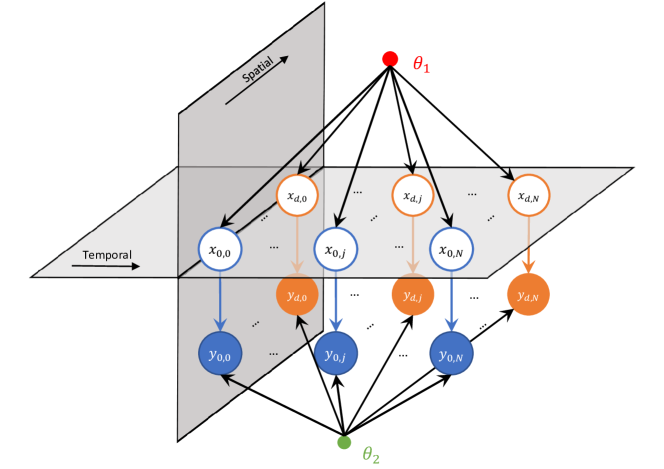
Figure 1: The general Bayesian network for traffic state estimation problem.

The traffic state of location $i$ at time $j$ is denoted by $x_{ij}$ as shown by the circle on the upper layer in the figure. $d$ and $N$ denote the number of locations and time slots being considered. The corresponding observation from the probe vehicles of each traffic state $x_{ij}$ is denoted by $y_{ij}$, which is represented by the circle on the lower layer. The traffic states depend on a set of parameters $\theta_{1}$, and the probe vehicle observations depend on both the traffic states and another set of parameters $\theta_{2}$. The parameters are shown as the small solid circles in the figure. The probabilistic framework represents a general traffic state estimation methodology. In order to demonstrate the universality of the framework, in the following paragraphs, we will discuss in detail some literature that conforms to this framework.

The first category of literature imposes independent assumptions, which implies the traffic states of different locations at different times are independent with each other. As an example, Comert and Cetin (2009) estimated the queue length in each cycle at an isolated and undersaturated intersection using probe vehicle data. The traffic state variable is the queue length, and the observation from probe vehicle data is the position of the last probe vehicle in the queue. Vehicle arrivals are assumed to follow a Poisson process, therefore, the parameter $\theta_{1}$ is the Poisson arrival rate. Given the queue length of a cycle, the observation also depends on the probe vehicle penetration rate which serves as parameter $\theta_{2}$. Similarly, studies by Zheng and Liu (2017), Zhao et al. (2019b), and Wang et al. (2019) also fall into this category.

The second category of literature includes those considering the temporal correlation (or spatial correlation) alone. Aljamal et al. (2020) proposed a Kalman filter (KF) based method to estimate the traffic state using probe vehicle data. The traffic state is the number of vehicles traversing the approach, and the corresponding probe vehicle observation is the probe vehicle travel time on the approach. The system dynamics are modeled as a linear system where the temporal correlation of traffic states is considered and incorporated. Therefore, parameter $\theta_{1}$ includes transition matrices of the model. For parameter $\theta_{2},$ it includes the measurement matrices, covariance of the measurement Gaussian noise, and the penetration rate. Besides the KF-based method, Wang et al. (2015) proposed a hidden Markov model (HMM) based method to estimate road segment’s travel speed using probe vehicle data, and it also belongs to this category.

The last category of literature involves those considering both spatial and temporal correlations. In addition to the queue length and traffic volume discussed earlier, the link travel time is studied in Herring et al. (2010). The traffic state of each link is represented by a discrete congestion level. For a given congestion level, the travel time distribution of that link is assumed to follow a Gaussian distribution. To capture the spatiotemporal correlation, the authors assume the state of a link at the next timestep depends on the states of the spatial neighbors in the current timestep. The observations are the link travel time obtained from the probe vehicle data. Therefore, parameter $\theta_{1}$ involves the state transition probability matrix and initial state probability. Parameter $\theta_{2}$ includes the mean and variance of the link travel time Gaussian distribution given different congestion levels. Similarly, the spatiotemporal correlation is also considered in Chen and Levin (2019) to estimate the occupancy of each road segment, and this method also falls into this category.

In summary, the proposed framework illustrated in Figure 1 represents a generic methodology for traffic state estimation problems. Based on the methodology, in the next sections, we will propose a probabilistic model for traffic volume reconstruction by fusing fixed-location sensor data and probe vehicle data.

3 Probabilistic models for traffic volume data in probe vehicle environments

Before delving into traffic volume reconstruction, we first describe the probabilistic models of whole-population traffic volumes and probe vehicle traffic volumes. By whole-population traffic volume, we refer to the total number of vehicles passing through a certain location at a certain time interval to distinguish it from the probe vehicle traffic volume. These probabilistic models are the traffic state and probe vehicle observation components in the framework that we introduced in the previous section. They serve as the foundation of the proposed data fusion method.

3.1 Distribution of whole-population traffic volumes based on the PPCA model

Following the same notation as in Section 2, for a specific time-of-day (TOD), we represent the traffic volumes of $d$ locations in $N$ days by a matrix $X\in\mathbb{R}^{d\times N}$, of which the element $x_{ij}$ represents the traffic volume at location $i$ on day $j$. Many studies have shown that the traffic volume data have strong spatiotemporal correlations and contain low-rank structures (Qu et al., 2009; Tan et al., 2013; Coogan et al., 2017; Feng et al., 2018). We apply the PPCA model proposed by Tipping and Bishop (1999) and Roweis and Ghahramani (1999) to capture the low-rank structure of the traffic volume data.

The PPCA model is a probabilistic model that generalizes PCA. The PPCA model assumes that the $d$-dimensional sample vector $x_{n}$, which is the $n$th column of $X$, depends on an $r$-dimensional latent vector $t_{n}$ through the following linear-Gaussian format

$$x_{n}=\Lambda t_{n}+\mu_{x}+\epsilon_{n},$$ (1)

where the latent vector $t_{n}$ is assumed to follow the multivariate Gaussian distribution $\mathcal{N}\left(0,I\right)$, and $\Lambda$ is a $d\times r$ projection matrix. $\mu_{x}$ is a vector that captures the mean of all samples, and $\epsilon_{n}$ is a $d$-dimensional isotropic Gaussian noise satisfying $\epsilon_{n}\sim\mathcal{N}\left(0,\sigma^{2}I\right)$, where $\sigma^{2}$ is the variance of the noise in each dimension. The intuition behind the formulation is that, with $r\ll d$, the original $d$-dimensional sample data can be represented in a more sparse way by mapping an $r$-dimensional latent variable in the latent variable space to the sample data space using the projection matrix $\Lambda$. According to the model, the distribution of $x_{n}$ is

$$x_{n}\sim\mathcal{N}\left(\mu_{x},\Lambda\Lambda^{T}+\sigma^{2}I\right).$$ (2)

Eq. (2) suggests that the distribution of traffic states depends on the parameter $\theta_{1}=\{\Lambda,\mu_{x},\sigma^{2}\}$, which includes the projection matrix, the mean vector, and the variance of the isotropic Gaussian noise.

3.2 Distribution of probe vehicle traffic volumes

The probe vehicle traffic volume represents the number of probe vehicles passing by a location in a specific period. Similarly, for a specific TOD, we represent the probe vehicle traffic volumes of $d$ locations in $N$ days by a matrix $Y$, which shares the same size as $X$. For location $i$ and day $j$, the probe vehicle traffic volume $y_{ij}$ is a fraction of the whole-population traffic volume $x_{ij}$.

We assume that the penetration rate of probe vehicles at each of the studied locations in the studied TOD is the same, denoted by $p$. We also assume probe vehicles are randomly mixed with regular vehicles. Based on the assumptions, given the penetration rate $p$ and the whole-population traffic volume $x_{ij}$, the traffic volume of probe vehicles at location $i$ on day $j$ follows the binomial distribution $y_{ij}|x_{ij}\sim\mathcal{B}\left(x_{ij},p\right)$. The binomial distribution can be well approximated by a Gaussian distribution when $x_{ij}$ is large (Shiryayev, 1984), which is adequate in our case. Therefore, the probe vehicle volume vector $y_{n}$ (the $n$th column of $Y$) approximately follows the Gaussian distribution

$$y_{n}\mid x_{n}\sim\mathcal{N}\left(x_{n}p,{\rm diag}\left(x_{n}p\left(1-p\right)\right)\right).$$ (3)

Another reason we approximate the binomial distribution using a Gaussian is that the PPCA framework applies to continuous random variables, whereas real-world traffic volumes are integer values. The Gaussian approximation makes it easy to consider the loop detector data and probe vehicle data together.

We also applied another approximation to the distribution of $y_{n}$, for mathematical simplification. We substitute the average traffic volume $\bar{x}=\sum_{i=1}^{N}x_{n}/N$ for the traffic volume $x_{n}$ in the variance of the distribution and decouple the mean and covariance by replacing $p\left(1-p\right)$ with $\eta^{2}$. Consequently, the probability distribution of the probe vehicle traffic volume is expressed as

$$y_{n}\mid x_{n}\sim\mathcal{N}\left(x_{n}p,\bar{x}\eta^{2}\right).$$ (4)

Therefore, the probe vehicle observation depends on the parameter $\theta_{2}=\{p,\eta^{2}\}$, where $p$ and $\eta^{2}$ denote the probe vehicle penetration rate and the decoupled variance, respectively.

4 Traffic volume reconstruction by data fusion

After modeling the distributions of whole-population traffic volumes and probe vehicle traffic volumes, in this section, we show how to fuse the loop detector data and probe vehicle data and how to infer the model parameters by solving an MLE problem. Once the parameters in the model are obtained, we will be able to reconstruct the unknown traffic volumes easily.

4.1 PPCA based data fusion

This paper focuses on the reconstruction of traffic volumes in two specific scenarios, i.e., the missing data scenario and the low coverage scenario. In the missing data scenario, some of the entries in $X$ might be missing due to loop detector malfunction or communication failure. The missing entries show a random pattern. In the low coverage scenario, loop detectors are not installed in some locations of our interest, and the entries of the corresponding rows in $X$ will be empty. Our goal is to reconstruct the missing values in $X$ by fusing the non-missing values in $X$ and the probe vehicle data $Y$.

In this study, we incorporate the probe vehicle data into the PPCA model and propose a PPCA-based data fusion (PPCA-DF) model. Following the notation in Marlin (2008), when there are missing elements in traffic volume data $x_{n}$, we divide $x_{n}$ into two parts $x_{n}^{m}$ and $x_{n}^{o}$, where $x_{n}^{m}$ refers to the missing part and $x_{n}^{o}$ represents the non-missing part. The available (non-missing) traffic volume data and probe vehicle data serve as the model input. For conciseness, we denote the collection of model parameters by $\theta=\left\{\Lambda,\mu_{x},\sigma^{2},p,\eta^{2}\right\}$. Given the non-missing traffic volume and probe vehicle volume data, the log-likelihood function of $\theta$ can be expressed as

$$\log\mathcal{L}\left(\theta;x_{n}^{o},y_{n}\right) =\sum_{n=1}^{N}\log P_{\theta}\left(x_{n}^{o},y_{n}\right)$$ (5)

$$=\sum_{n=1}^{N}\log\left(\int P_{\theta}\left(x_{n}^{m},x_{n}^{o},y_{n}\right)dx_{n}^{m}\right)$$ (6)

$$=\sum_{n=1}^{N}\log\left(\int\int P_{\theta}\left(x_{n}^{m},x_{n}^{o},y_{n},t_{n}\right)dx_{n}^{m}dt_{n}\right).$$ (7)

The objective function of the PPCA-DF model is to maximize the log-likelihood function. For the convenience of the solving process, we introduce the latent vector $t_{n}$ to the objective function as shown in Eq. (7).

The complete-data likelihood function in the marginal log-likelihood function (7) can be expressed as

$$P_{\theta}\left(x_{n}^{m},x_{n}^{o},y_{n},t_{n}\right) =P_{\theta}\left(x_{n},y_{n},t_{n}\right)$$ (8)

$$=P_{\theta}\left(t_{n}\right)P_{\theta}\left(x_{n}\rvert t_{n}\right)P_{\theta}\left(y_{n}\rvert x_{n},t_{n}\right)$$ (9)

$$=P_{\theta}\left(t_{n}\right)P_{\theta}\left(x_{n}\rvert t_{n}\right)P_{\theta}\left(y_{n}\rvert x_{n}\right).$$ (10)

The last step in the derivation is because $y_{n}$ is independent of $t_{n}$ given $x_{n}$. The probability density functions of $t_{n}$, $x_{n}\rvert t_{n}$, and $y_{n}\rvert x_{n}$ under parameter $\theta$ are

$$P_{\theta}\left(t_{n}\right) =\left(2\pi\right)^{-\frac{r}{2}}e^{-\frac{1}{2}t_{n}^{T}t_{n}},$$ (11)

$$P_{\theta}\left(x_{n}\rvert t_{n}\right) =\left(2\pi\sigma^{2}\right)^{-\frac{d}{2}}e^{-\frac{1}{2\sigma^{2}}\left(x_{n}-\Lambda t_{n}-\mu_{x}\right)^{T}\left(x_{n}-\Lambda t_{n}-\mu_{x}\right)},$$ (12)

$$P_{\theta}\left(y_{n}\rvert x_{n}\right) =\frac{1}{\sqrt{\text{$\Pi_{i=1}^{d}\bar{x}_{i}$}}}\left(2\pi\eta^{2}\right)^{-\frac{d}{2}}e^{-\frac{1}{2}\left(y_{n}-px_{n}\right)^{T}\left[{\rm diag}\left(\bar{x}\eta^{2}\right)\right]^{-1}\left(y_{n}-px_{n}\right)},$$ (13)

respectively. Please note that $\bar{x}$ in Eq. (13) is prior information that can be obtained by averaging the non-missing values.

By substituting these probability density functions into Eq. (10), the complete-data log-likelihood function can be expressed as

$$\log P_{\theta}\left(x_{n}^{m},x_{n}^{o},y_{n},t_{n}\right) =-\frac{\left(r+2d\right)}{2}\log\left(2\pi\right)-\frac{1}{2}t_{n}^{T}t_{n}-\frac{d}{2}\log\left(\sigma^{2}\right)$$

$$-\frac{1}{2\sigma^{2}}\left(x_{n}-\Lambda t_{n}-\mu_{x}\right)^{T}\left(x_{n}-\Lambda t_{n}-\mu_{x}\right)-\frac{1}{2}\sum_{i=1}^{d}\log\left(\bar{x}_{i}\eta^{2}\right)$$

$$-\frac{1}{2}\left(y_{n}-px_{n}\right)^{T}\left[{\rm diag}\left(\bar{x}\eta^{2}\right)\right]^{-1}\left(y_{n}-px_{n}\right).$$ (14)

Substituting Eq. (14) into Eq. (7) gives a non-concave objective function of the maximum likelihood estimation problem. Therefore, we apply the EM algorithm (Dempster et al., 1977) to solve it.

4.2 EM algorithm

4.2.1 E-step

The goal of the EM algorithm is to find maximum likelihood solutions for models having latent variables (Bishop, 2006). In the E-step, we evaluate the expectation of the complete-data log-likelihood function under the posterior distribution of the latent variables given the current estimate $\theta^{(k)}$, where the superscript $k$ is the index denoting for current iteration. Mathematically, the expectation can be expressed as $\mathbb{E}_{t_{n},x_{n}^{m}\rvert x_{n}^{o},y_{n},\theta^{(k)}}\left[\log\mathcal{L}\left(\theta;x_{n},y_{n},t_{n}\right)\right]$, where $\log\mathcal{L}\left(\theta;x_{n},y_{n},t_{n}\right)={\rm log}P_{\theta}\left(x_{n},y_{n},t_{n}\right)$.

To get the probability density function of the posterior distribution under parameter $\theta^{(k)}$, we first derive the joint distribution of $x_{n},y_{n}$ and $t_{n}$, which is

$$\left(x_{n},y_{n},t_{n}\right);\theta^{(k)}\sim\mathcal{N}\left(\left[\begin{array}[]{c}\mu_{x}^{(k)}\\ \mu_{y}^{(k)}\\ 0\end{array}\right],\left[\begin{array}[]{ccc}\Sigma_{x_{n}x_{n}}^{(k)}&\Sigma_{x_{n}y_{n}}^{(k)}&\Sigma_{x_{n}t_{n}}^{(k)}\\ \Sigma_{y_{n}x_{n}}^{(k)}&\Sigma_{y_{n}y_{n}}^{(k)}&\Sigma_{y_{n}t_{n}}^{(k)}\\ \Sigma_{t_{n}x_{n}}^{(k)}&\Sigma_{t_{n}y_{n}}^{(k)}&\Sigma_{t_{n}t_{n}}^{(k)}\end{array}\right]\right),$$ (15)

where the covariance matrix can be expressed as

$$\left[\begin{array}[]{ccc}(\sigma^{2})^{\left(k\right)}I+\Lambda^{\left(k\right)}\left(\Lambda^{\left(k\right)}\right)^{T}&p^{\left(k\right)}\left((\sigma^{2})^{\left(k\right)}I+\Lambda^{\left(k\right)}\left(\Lambda^{\left(k\right)}\right)^{T}\right)&\Lambda^{\left(k\right)}\\ p^{\left(k\right)}\left((\sigma^{2})^{\left(k\right)}I+\Lambda^{\left(k\right)}\left(\Lambda^{\left(k\right)}\right)^{T}\right)^{T}&{\rm diag}\left(\bar{x}(\eta^{2})^{\left(k\right)}\right)+\left(p^{\left(k\right)}\right)^{2}\left((\sigma^{2})^{\left(k\right)}I+\Lambda^{\left(k\right)}\left(\Lambda^{\left(k\right)}\right)^{T}\right)&p^{\left(k\right)}\Lambda^{\left(k\right)}\\ \left(\Lambda^{\left(k\right)}\right)^{T}&p^{\left(k\right)}\left(\Lambda^{\left(k\right)}\right)^{T}&I\end{array}\right].$$ (19)

Then, according to the Gaussian conditional distribution formula, the conditional distribution of the latent variables $x_{n}^{m}$ and $t_{n}$ given the observed data $x_{n}^{o}$ and $y_{n}$ is still Gaussian. For conciseness, we denote the distribution of $\left(t_{n},x_{n}^{m}\rvert x_{n}^{o},y_{n};\theta^{(k)}\right)$ by $q_{n}^{(k)}\left(t_{n},x_{n}^{m}\right)$, that is

$$q_{n}^{(k)}\left(t_{n},x_{n}^{m}\right):t_{n},x_{n}^{m}\rvert x_{n}^{o},y_{n};\theta^{(k)}\sim\mathcal{N}\left(\left[\begin{array}[]{c}\mu_{t_{n}\rvert x_{n}^{o},y_{n}}^{(k)}\\ \mu_{x_{n}^{m}\rvert x_{n}^{o},y_{n}}^{(k)}\end{array}\right],\left[\begin{array}[]{cc}\Sigma_{t_{n}\rvert x_{n}^{o},y_{n}}^{(k)}&\Sigma_{t_{n}x_{n}^{m}\rvert x_{n}^{o},y_{n}}^{(k)}\\ \left(\Sigma_{t_{n}x_{n}^{m}\rvert x_{n}^{o},y_{n}}^{(k)}\right)^{T}&\Sigma_{x_{n}^{m}\rvert x_{n}^{o},y_{n}}^{(k)}\end{array}\right]\right).$$ (20)

Finally, we evaluate the expected complete-data log-likelihood function under the posterior distribution $q_{n}^{(k)}(t_{n},x_{n}^{m})$, which is

$$\mathbb{E}_{q_{n}^{(k)}}\left[\mathcal{\log L}\left(\theta;x_{n},y_{n},t_{n}\right)\right] =\int\int q_{n}^{(k)}\left(t_{n},x_{n}^{m}\right)\left(\log P\left(t_{n}\right)+\log P\left(x_{n}\rvert t_{n}\right)+\log P\left(y_{n}\rvert x_{n}\right)\right)dx_{n}^{m}dt_{n}$$

$$=-\frac{\left(r+2d\right)}{2}\log\left(2\pi\right)-\frac{1}{2}\mathbb{E}_{q_{n}^{(k)}}\left[t_{n}^{T}t_{n}\right]-\frac{d}{2}\log\left(\sigma^{2}\right)$$

$$-\frac{1}{2\sigma^{2}}\mathbb{E}_{q_{n}^{(k)}}\left[\left(x_{n}-\Lambda t_{n}-\mu_{x}\right)^{T}\left(x_{n}-\Lambda t_{n}-\mu_{x}\right)\right]-\frac{1}{2}\sum_{i=1}^{d}\log\left(\bar{x}_{i}\eta^{2}\right)$$

$$-\frac{1}{2}\mathbb{E}_{q_{n}^{(k)}}\left[\left(y_{n}-px_{n}\right)^{T}\left[{\rm diag}\left(\bar{x}\eta^{2}\right)\right]^{-1}\left(y_{n}-px_{n}\right)\right].$$ (21)

4.2.2 M-step

In the M-step, considering all the available loop detector and probe vehicle data, we maximize the sum of the expected complete log-likelihood function in terms of the parameters $\theta$, which is

$$Q\left(\theta;\theta^{(k)}\right)=\sum_{n=1}^{N}\mathbb{E}_{q_{n}^{(k)}}\left[\log\mathcal{L}\left(\theta;x_{n},y_{n},t_{n}\right)\right].$$ (22)

The solutions to the optimization problem yield the update rules of the parameters, which are

$$\mu_{x}^{\left(k+1\right)}=\frac{1}{N}\sum_{n=1}^{N}\left(\mathbb{E}_{q_{n}^{(k)}}\left[x_{n}\right]-\Lambda^{\left(k\right)}\mathbb{E}_{q_{n}^{(k)}}\left[t_{n}\right]\right),$$ (23)

$$\Lambda^{\left(k+1\right)}=\left(\sum_{n=1}^{N}\left(\mathbb{E}_{q_{n}^{(k)}}\left[x_{n}t_{n}^{T}\right]-\mu_{x}^{\left(k\right)}\mathbb{E}_{q_{n}^{(k)}}\left[t_{n}\right]^{T}\right)\right)\left(\sum_{n=1}^{N}\mathbb{E}_{q_{n}^{(k)}}\left[t_{n}t_{n}^{T}\right]\right)^{-1},$$ (24)

$$\left(\sigma^{2}\right)^{\left(k+1\right)} =\frac{1}{Nd}\sum_{n=1}^{N}\left({\rm tr}\left(\mathbb{E}_{q_{n}^{(k)}}\left[x_{n}x_{n}^{T}\right]\right)+\left(\mu_{x}^{\left(k\right)}\right)^{T}\mu_{x}^{\left(k\right)}+{\rm tr}\left(\left(\Lambda^{\left(k\right)}\right)^{T}\Lambda^{\left(k\right)}\mathbb{E}_{q_{n}^{(k)}}\left[t_{n}t_{n}^{T}\right]\right)\right.$$

$$\left.-2\left(\mu_{x}^{\left(k\right)}\right)^{T}\mathbb{E}_{q_{n}^{(k)}}\left[x_{n}\right]-2{\rm tr}\left(\Lambda^{\left(k\right)}\mathbb{E}_{q_{n}^{(k)}}\left[x_{n}t_{n}^{T}\right]^{T}\right)+2\left(\mu_{x}^{\left(k\right)}\right)^{T}\Lambda^{\left(k\right)}\mathbb{E}_{q_{n}^{(k)}}\left[t_{n}\right]\right),$$ (25)

$$p^{(k+1)}=\left(\sum_{n=1}^{N}y_{n}^{T}{\rm diag}\left(\bar{x}\left(\eta^{2}\right){}^{\left(k\right)}\right)^{-1}\mathbb{E}_{q_{n}^{(k)}}\left[x_{n}\right]\right)\left(\sum_{n=1}^{N}{\rm tr}\left(\mathbb{E}_{q_{n}^{(k)}}\left[x_{n}x_{n}^{T}\right]{\rm diag}\left(\bar{x}\left(\eta^{2}\right){}^{\left(k\right)}\right)^{-1}\right)\right)^{-1},$$ (26)

$$\left(\eta^{2}\right)^{(k+1)}=\frac{1}{Nd}\sum_{n=1}^{N}\sum_{i=1}^{d}\frac{1}{\bar{x}_{i}}\left(y_{ni}^{2}-2p^{\left(k\right)}y_{ni}\mathbb{E}_{q_{n}^{(k)}}\left[x_{n}\right]_{i}+\left(p^{\left(k\right)}\right)^{2}\mathbb{E}_{q_{n}^{(k)}}\left[x_{n}x_{n}^{T}\right]_{ii}\right).$$ (27)

The solutions are concisely expressed in terms of five expectations derived from Eq. (20). The detailed solving process and the expressions of the expectations are in Appendix A.

4.3 Estimating the unknown traffic volumes

Performing the update rules introduced above iteratively leads to the convergence of the estimated $\theta$ (Dempster et al., 1977). With the estimated parameters of the PPCA-DF model, the posterior predictive distribution of the unknown data is a Gaussian distribution given by

$$x_{n}^{m}\rvert x_{n}^{o},y_{n}\sim\mathcal{N}\left(\mu_{x_{n}^{m}\rvert x_{n}^{o},y_{n}},\Sigma_{x_{n}^{m}\rvert x_{n}^{o},y_{n}}\right),$$ (28)

where

$$\mu_{x_{n}^{m}\rvert x_{n}^{o},y_{n}} =\mu_{x_{n}^{m}}+\left[\begin{array}[]{cc}\Sigma_{x_{n}^{m}x_{n}^{o}}&\Sigma_{x_{n}^{m}y}\end{array}\right]\left[\begin{array}[]{cc}\Sigma_{x_{n}^{o}x_{n}^{o}}&\Sigma_{x_{n}^{o}y_{n}}\\ \Sigma_{y_{n}x_{n}^{o}}&\Sigma_{y_{n}y_{n}}\end{array}\right]^{-1}\left(\left[\begin{array}[]{c}x_{n}^{o}\\ y_{n}\end{array}\right]-\left[\begin{array}[]{c}\mu_{x_{n}^{o}}\\ \mu_{y}\end{array}\right]\right),$$ (36)

$$\Sigma_{x_{n}^{m}\rvert x_{n}^{o},y_{n}} =\Sigma_{x_{n}^{m}x_{n}^{m}}-\left[\begin{array}[]{cc}\Sigma_{x_{n}^{m}x_{n}^{o}}&\Sigma_{x_{n}^{m}y_{n}}\end{array}\right]\left[\begin{array}[]{cc}\Sigma_{x_{n}^{o}x_{n}^{o}}&\Sigma_{x_{n}^{o}y_{n}}\\ \Sigma_{y_{n}x_{n}^{o}}&\Sigma_{y_{n}y_{n}}\end{array}\right]^{-1}\left[\begin{array}[]{cc}\Sigma_{x_{n}^{m}x_{n}^{o}}&\Sigma_{x_{n}^{m}y_{n}}\end{array}\right]^{T}.$$ (41)

Therefore, we can estimate the unknown traffic volumes in the $n$th column of $X$ by the mean $\mu_{x_{n}^{m}\rvert x_{n}^{o},y_{n}}$.

5 Case studies

In this section, we first introduce the dataset we use for validation. Then, we validate the proposed method in different scenarios and compare its performance with the baseline methods.

5.1 Ground-truth dataset

To examine the performance of the proposed PPCA-DF model in both the missing data scenario and the low coverage scenario, we conduct experiments using a real-world traffic volume dataset. The ground-truth dataset used here is the PORTAL Arterial Data (https://portal.its.pdx.edu/fhwa) collected from the loop detectors on 82nd Avenue in Portland, Oregon. The IDs of the specific 15 loop detectors we use are 253, 254, 255, 256, 409, 410, 411, 412, 414, 415, 416, 712, 713, 714, and 715. The locations of the loop detectors along 82nd Avenue are shown in Figure 2. Because of the data availability, we choose four intersections (Intersection 1 to Intersection 4 shown on Figure 2) spanning roughly 6.5 miles apart. We use the data of 15 workdays from October 21 to November 10, 2011. We aggregate the data to 15-min intervals in the preprocessing stage. Figure 3 shows the average traffic volumes in different TODs over the 15 workdays collected by the 15 loop detectors. In general, the traffic volumes at different locations fluctuate in a similar trend over time, which implies a strong correlation.

Figure 2: Ground-truth dataset locations.

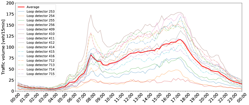
Figure 3: The average traffic volumes over the 15 workdays at different locations and TODs.

5.2 Experimental settings

5.2.1 Probe vehicle data

Since we do not have access to the real-world probe vehicle data collected from the studied locations at the same time, for validation purposes, we simulate the probe vehicle data by randomly sampling from the whole-population traffic volume data. For each vehicle recorded by the loop detectors, we randomly determine if it is a probe vehicle or a regular vehicle according to the penetration rate $p$. After this step, we obtain the simulated probe vehicle data, which are further converted into the probe vehicle traffic volume matrix $Y$.

5.2.2 Traffic volume data with missing entries

We simulate two missing data patterns to characterize the two different scenarios of our interest, i.e., the missing data scenario and the low coverage scenario. For the missing data scenario, given a missing ratio, we perform a Bernoulli trial to decide if each entry in the ground-truth traffic volume matrix is missing or not. If the random sampling process shows the entry is missing, we will hide the value of the entry. This process simulates the loop detector malfunction situation. For the low coverage scenario, we randomly remove several rows of the ground-truth traffic volume matrix. This process simulates the situation where some of the studied locations are not covered by loop detectors. After this step, we obtain the simulated loop detector traffic volume matrix $X$. In this case study, for each TOD, the size of $X$ and $Y$ is $15\times 15$, as there are 15 loop detectors and 15 days. The loop detector traffic volume matrix $X$ (with missing entries or rows), together with the probe vehicle traffic volume matrix $Y$, will serve as the input to our proposed model.

5.3 Measure of accuracy

We evaluate the performance of the proposed method by the root mean square error (RMSE) when reconstructing the missing entries. The traffic volumes are reconstructed for each TOD separately. Then, we calculate the performance measure for each TOD, or combine results for all TODs to get the overall performance measurement.

5.4 Results for the missing data scenario

Figure 4 illustrates the estimation process in the missing data scenario. The input data include the loop detector data $X$ with randomly missing entries and the probe vehicle traffic volume matrix $Y$. The colors represent different magnitudes of traffic volumes. The entries with traffic volumes equal to zero correspond to those entries with missing data. Using the proposed PPCA-DF model, we can reconstruct the missing traffic volumes.

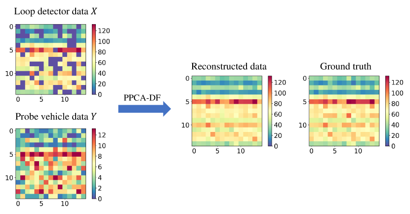
Figure 4: Traffic volume reconstruction for the missing data scenario.

The dimension of the projection matrix $\Lambda$ is $d\times r$, where $r$ is the rank of the matrix. Intuitively, increasing the rank of the projection matrix can capture more spatiotemporal correlations in the traffic volume data. However, increasing the rank may also increase the model complexity and result in overfitting. In the case study, we consider the traffic volume reconstruction for 15-min intervals. Due to the small granularity, the variance of the probe vehicle traffic volume is relatively large. As a result, if the rank is too large, the noise in data will be introduced to the model. This effect is particularly critical during the night time, when the ground-truth traffic volume is very small and the number of observed probe vehicles fluctuate significantly. Therefore, after doing the cross-validation process, we set $r=1$. In other settings, for example, when we reconstruct 60-min traffic volumes, increasing the rank might give rise to better performance.

5.4.1 The impact of missing ratios and penetration rates

In this section, we examine the impact of missing ratios and penetration rates on the PPCA-DF model in the missing data scenario. We enumerate the missing ratio from 5% to 95%, with a step size of 5%. At the same time, we test the method under different penetration rates, including 5%, 10%, 20%, and 50%. For each test, we run 30 independent experiments and then calculate the average performance measurement.

Figure 5 shows the results. In general, the estimation accuracy decreases as the missing ratio increases. It is because when the missing ratio is low, non-missing entries can provide abundant information. By contrast, when the missing ratio is high, the number of remaining entries is very limited, which makes it challenging to estimate the unknown traffic volumes. Even though, the proposed model can still give an accurate estimation when the missing ratio is higher than 80%, which validates the robustness of our approach. Overall, the proposed method is not very sensitive to the missing ratio. It is due to the benefits of fusing the loop detector data and probe vehicle data. Probe vehicles cover a broad range of locations and provide a partial observation of the traffic volumes, whereas loop detectors measure the traffic volumes at several discrete locations. Even though the missing ratio is high and many entries are missing, we can still estimate the corresponding traffic volumes by exploiting the spatiotemporal correlations contained in the two data sources.

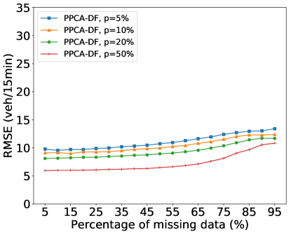
Figure 5: Performance of the proposed method under different missing ratios and different penetration rates in the missing data scenario.

The probe vehicle penetration rate is another critical parameter that influences the performance of the method. It determines the magnitude of the probe vehicle traffic volumes. With a higher penetration rate, the spatiotemporal correlation of the traffic volume data can be better retained in the probe vehicle data. Even though, the results in Figure 5 show that the proposed method can already reconstruct traffic volumes accurately when the penetration rate is only 10%. These results indicate the feasibility of practical applications of our approach, as some studies have already shown that the probe vehicle penetration rate could reach 10% in some places (Zheng and Liu, 2017; Zhao et al., 2019a, b). For illustration purposes, we will use 10% as the penetration rate in the following experiments.

5.4.2 Comparison with existing methods

We compare the proposed PPCA-DF model with two baseline methods. The first one is the direct scaling method, which reconstructs the unknown traffic volumes by scaling up the traffic volumes of the probe vehicles using the penetration rate directly (Wong et al., 2019). The second method is the PPCA method used by Qu et al. (2009) and Li et al. (2013), which captures the low-rank structure by solving an MLE problem. For the PPCA method, it only uses the loop detector data to construct the low-rank structure of the traffic volume data and then uses it for missing value imputation. It also needs to determine the dimension of the projection matrix. We choose the dimension that yields the best performance, which is also $r=1$ for the 15-min interval case.

The comparison results are shown in Figure 6. As the results suggest, the proposed method consistently outperforms the two baseline methods under different missing ratios. For the direct scaling method, it only utilizes the probe vehicle data, so the estimation accuracy does not depend on the missing ratio. Scaling up the probe vehicle traffic volume directly will amplify its variance, especially when the penetration rate is not high enough or when the magnitude of traffic volume is low (e.g., at the night time). However, the direct scaling method does not use any information from other locations and time slots to reduce the variance. Therefore, the RMSE is relatively large. The proposed method also yields better performance than the PPCA method for all missing ratios. Especially when the missing ratio is high, the PPCA baseline method cannot reconstruct the missing values accurately with limited information. The reason is that, when the missing ratio is high, many entries in the loop detector data are missing, which severely undermines the spatiotemporal correlation the traffic volume data should have. The PPCA-DF model proposed in this paper, however, tries to find the low-rank representation of the traffic volumes by combining both of the data sources, which gives rise to better estimation accuracy. The results imply that the probe vehicle data is an appropriate data source for finding the embedded spatiotemporal correlations. It also validates the idea that incorporating probe vehicle data can provide a robust approach to the reconstruction of traffic volumes.

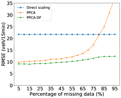
Figure 6: Comparison of different methods for the missing data scenario.

We further examine the estimation accuracy of the methods in different TODs. Figure 7a shows the estimation results of different methods. The figure corresponds to the scenario where the percentage of missing data is 50%. The proposed method outperforms the direct scaling and PPCA baseline methods in almost all the TODs. The RMSE is smaller in the night time compared to the day time, because the ground-truth traffic volumes are much smaller in the night time, as shown in Figure 3. The mean absolute percentage error (MAPE) is actually smaller in the day time as shown in Figure 7b, due to the larger sample size of probe vehicle data and high spatiotemporal correlation. The results show that the MAPE is around 13% in the day time (9:00-17:00), which suggests good estimation accuracy for 15-min traffic volumes.

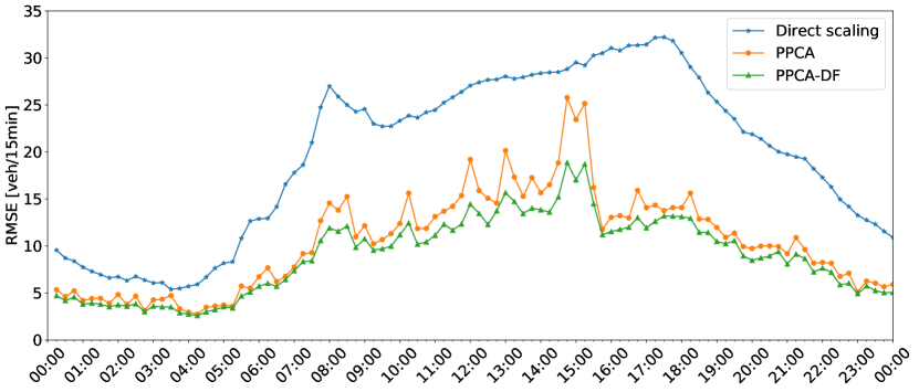
(a)

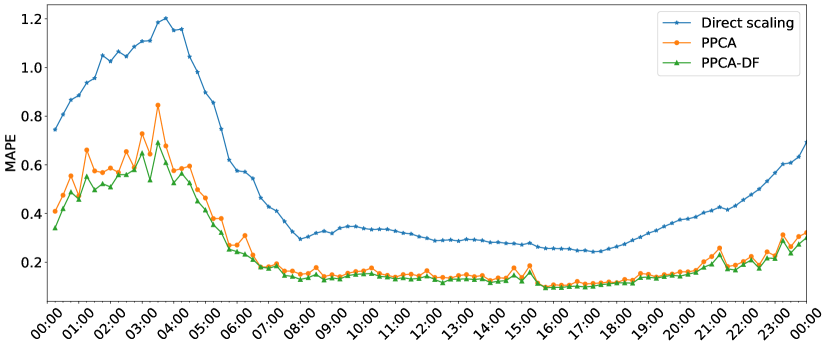
(b)

Figure 7: Estimation accuracy of different methods in different TODs for the missing data scenario measured by: (a) RMSE and (b) MAPE.

5.5 Results for the low coverage scenario

The low coverage scenario is more challenging. In this case, not all the locations we study are covered by loop detectors. In other words, several rows of the traffic volume matrix $X$ can be missing. Figure 8 illustrates the whole process of traffic volume reconstruction for the low coverage scenario. Similar to the missing data scenario, the input data include the loop detector data $X$ with some missing rows and the probe vehicle data $Y$. The unknown traffic volumes can be reconstructed using the proposed PPCA-DF model.

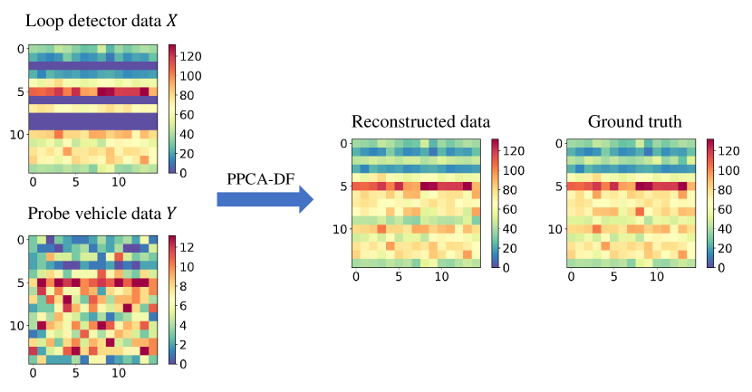
Figure 8: Traffic volume reconstruction for the low coverage scenario.

5.5.1 The impact of missing ratios and penetration rates

We first evaluate the performance of the proposed model under different missing ratios and different levels of probe vehicle market penetration. Figure 9 shows the results. Similar to the missing data scenario, generally speaking, a lower missing ratio or a higher penetration rate leads to better estimation accuracy. The results suggest that a 10% penetration rate can still enable the proposed method to reconstruct traffic volumes accurately, even when multiple locations are not covered with loop detectors. Again, considering the current situations of probe vehicle deployment, we will still use the 10% penetration rate in the following experiments.

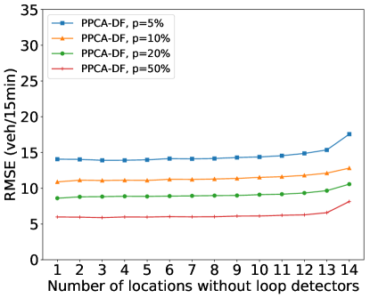
Figure 9: Performance of the proposed method under different missing ratios and different penetration rates in the low coverage scenario.

From the results, we can also find that when there are more locations not covered by loop detectors, the estimation accuracy does not decrease drastically, which again demonstrates the robustness of the proposed method. It is still because of the benefits of involving the probe vehicle data source. Although many locations are not covered by loop detectors, the spatiotemporal correlation can be captured by probe vehicle data which covers all locations. Therefore, by leveraging data fusion, we can still accurately estimate the corresponding traffic volumes. It implies that the probe vehicle data is a valuable complement to the traditional loop detector data, and it can help us better understand the traffic flows at the network level.

5.5.2 Comparison with existing methods

Since the PPCA method used in Qu et al. (2009) and Li et al. (2013) cannot deal with the low coverage scenario, we only compare the proposed PPCA-DF model with the direct scaling method. As shown in Figure 10, the proposed method performs significantly better than the baseline method. It is because the proposed method considers the spatiotemporal correlation in the traffic volume data, whereas the direct scaling method considers each location and each time slot independently.

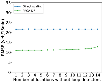
Figure 10: Comparison of different methods for the low coverage scenario.

Figure 11 shows the estimation results of different methods in different TODs. The figure corresponds to the scenario when seven randomly chosen locations are not covered by loop detectors. The proposed method outperforms the direct scaling method in all the TODs. The MAPE is around 15% in the day time (9:00-17:00), which validates the performance of the proposed method in the low coverage scenario.

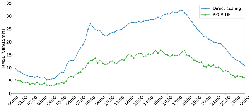
(a)

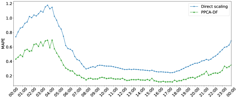
(b)

Figure 11: Estimation accuracy of different methods in different TODs for the low coverage scenario measured by: (a) RMSE and (b) MAPE.

6 Conclusions

In this paper, we first propose a general probabilistic framework for traffic state estimation problems. Based on the framework, we propose a data fusion model PPCA-DF, which can reconstruct the unknown traffic volumes by exploiting the spatiotemporal correlations of traffic volumes. The proposed PPCA-DF model considers both loop detector data and probe vehicle data when inferring the low-rank structure using maximum likelihood estimation. The PPCA-DF model can handle two critical and frequently occurring scenarios. The first scenario is the missing data scenario, where some traffic volume data are missing due to loop detector malfunction or communication failure. This problem has long been commonly recognized as a shortcoming of loop detectors. The second scenario is the low coverage scenario, where no loop detectors are installed at some locations of our interest. This scenario also frequently occurs, since fixed-location sensors usually can only cover a small subset of links in the transportation network due to the high installation and maintenance costs. Whereas most of the existing literature focuses on the first scenario and cannot handle the second scenario, the proposed PPCA-DF model can be applied to both scenarios.

We examine the performance of the proposed method using a real-world loop detector dataset collected from Portland, Oregon. The results show that the PPCA-DF model can achieve good performance when dealing with both of the two scenarios. It can outperform the existing methods even when the penetration rate of probe vehicles is only 10%. What is more, the proposed model is not sensitive to the missing ratio and can give accurate estimation results when the missing ratio is higher than 80% or when most locations have no loop detectors installed. These results validate the effectiveness and robustness of the proposed model and also imply its potential for practical applications.

The current work can be extended in a few directions by future research. For instance, firstly, we only count the number of probe vehicles passing by a certain location and use the aggregated information in the model. However, the probe vehicle data include the complete trajectories of the vehicles, which contain rich information. The estimation accuracy could be further improved by considering more detailed information encoded in the trajectory, such as the arrival time of each probe vehicle. Secondly, we assume that the penetration rate of probe vehicles at each of the studied locations is the same in the same TOD. The assumption can be relaxed by considering the penetration rate as a random variable following a certain distribution. It will give more flexibility to the model and can therefore capture the daily variance of the penetration rate. Thirdly, in this study, we assume the observed loop detector volume is the ground-truth traffic volume. However, in a real-world situation, measurement errors for the loop detector do exist, and the errors should also be considered.

Appendix A

The analytical solutions of the EM algorithm can be obtained by setting the derivatives of $Q\left(\theta;\theta^{(k)}\right)$ to zero, i.e.,

$$\frac{\partial Q\left(\theta\mid\theta^{(k)}\right)}{\partial\mu_{x}}=\sum_{n=1}^{N}\frac{1}{\left(\sigma^{2}\right)^{\left(k\right)}}\left(\mathbb{E}_{q_{n}^{(k)}}\left[x_{n}\right]-\Lambda^{\left(k\right)}\mathbb{E}_{q_{n}^{(k)}}\left[t_{n}\right]-\mu_{x}\right)=0,$$ (42)

$$\frac{\partial Q\left(\theta\mid\theta^{(k)}\right)}{\partial\Lambda}=\sum_{n=1}^{N}\frac{1}{\left(\sigma^{2}\right)^{\left(k\right)}}\left(\mathbb{E}_{q_{n}^{(k)}}\left[\left(x_{n}-\mu_{x}^{(k)}\right)t_{n}^{T}\right]-\Lambda\mathbb{E}_{q_{n}^{(k)}}\left[t_{n}t_{n}^{T}\right]\right)=0,$$ (43)

$$\frac{\partial Q\left(\theta\mid\theta^{(k)}\right)}{\partial\sigma^{2}}=\sum_{n=1}^{N}\left(\frac{d}{\sigma^{2}}-\frac{1}{\sigma^{4}}\mathbb{E}_{q_{n}^{(k)}}\left[\left(x_{n}-\Lambda^{\left(k\right)}t_{n}-\mu_{x}^{(k)}\right)^{T}\left(x_{n}-\Lambda^{\left(k\right)}t_{n}-\mu_{x}^{(k)}\right)\right]\right)=0,$$ (44)

$$\frac{\partial Q\left(\theta\mid\theta^{(k)}\right)}{\partial p}=\sum_{n=1}^{N}\mathbb{E}_{q_{n}^{(k)}}\left[\left({\rm diag}\left(\bar{x}\left(\eta^{2}\right){}^{\left(k\right)}\right)^{-1}\left(y_{n}-px_{n}\right)\right)^{T}x_{n}\right]=0,$$ (45)

$$\frac{\partial Q\left(\theta\mid\theta^{(k)}\right)}{\partial\eta^{2}}=\sum_{n=1}^{N}\left(\frac{d}{\eta^{2}}-\frac{1}{\eta^{4}}\mathbb{E}_{q_{n}^{(k)}}\left[\left(y_{n}-p^{\left(k\right)}x_{n}\right)^{T}{\rm diag}\left(\bar{x}\right)^{-1}\left(y_{n}-p^{\left(k\right)}x_{n}\right)\right]\right)=0.$$ (46)

Solving the equations above yields the update rules of the parameters, i.e., Eqs. (23)-(27). The explicit expressions of the five expectations are shown as below.

$$\mathbb{E}_{q_{n}^{(k)}}\left[x_{n}\right]=\left[\begin{array}[]{c}\mu_{x_{n}^{m}\rvert x_{n}^{o},y_{n}}^{(k)}\\ x_{n}^{o}\end{array}\right],$$ (47)

$$\mathbb{E}_{q_{n}^{(k)}}\left[t_{n}\right]=\mu_{t_{n}\rvert x_{n}^{o},y_{n}}^{(k)},$$ (48)

$$\mathbb{E}_{q_{n}^{(k)}}\left[t_{n}t_{n}^{T}\right]=\Sigma_{t_{n}\rvert x_{n}^{o},y_{n}}^{(k)}+\mu_{t_{n}\rvert x_{n}^{o},y_{n}}^{(k)}\left(\mu_{t_{n}\rvert x_{n}^{o},y_{n}}^{(k)}\right)^{T},$$ (49)

$$\mathbb{E}_{q_{n}^{(k)}}\left[x_{n}x_{n}^{T}\right]=\left[\begin{array}[]{cc}\Sigma_{x_{n}^{m}\rvert x_{n}^{o},y_{n}}^{\left(k\right)}+\mu_{x_{n}^{m}\rvert x_{n}^{o},y_{n}}^{(k)}\left(\mu_{x_{n}^{m}\rvert x_{n}^{o},y_{n}}^{(k)}\right)^{T}&\mu_{x_{n}^{m}\rvert x_{n}^{o},y_{n}}^{(k)}\left(x_{n}^{o}\right)^{T}\\ x_{n}^{o}\left(\mu_{x_{n}^{m}\rvert x_{n}^{o},y_{n}}^{(k)}\right)^{T}&x_{n}^{o}\left(x_{n}^{o}\right)^{T}\end{array}\right],$$ (50)

$$\mathbb{E}_{q_{n}^{(k)}}\left[x_{n}t_{n}^{T}\right]=\left[\begin{array}[]{c}\Sigma_{x_{n}^{m}t_{n}\rvert x_{n}^{o},y_{n}}^{(k)}+\mu_{x_{n}^{m}\rvert x_{n}^{o},y_{n}}^{(k)}\left(\mu_{t_{n}\rvert x_{n}^{o},y_{n}}^{(k)}\right)^{T}\\ x_{n}^{o}\left(\mu_{t_{n}\rvert x_{n}^{o},y_{n}}^{(k)}\right)^{T}\end{array}\right].$$ (51)

CRediT author statement

Xintao Yan: Conceptualization, Methodology, Software, Data curation, Writing-original draft, Writing-review and editing. Yan Zhao: Conceptualization, Methodology, Software, Data curation, Writing-original draft, Writing-review and editing. Henry X. Liu: Conceptualization, Writing-review and editing, Funding acquisition, Supervision.

References

- Aljamal et al. (2020) Aljamal, M.A., Abdelghaffar, H.M., Rakha, H.A., 2020. Real-time estimation of vehicle counts on signalized intersection approaches using probe vehicle data. IEEE Transactions on Intelligent Transportation Systems doi:10.1109/TITS.2020.2973954.
- Asif et al. (2016) Asif, M.T., Mitrovic, N., Dauwels, J., Jaillet, P., 2016. Matrix and tensor based methods for missing data estimation in large traffic networks. IEEE Transactions on Intelligent Transportation Systems 17, 1816–1825.
- Bae et al. (2018) Bae, B., Kim, H., Lim, H., Liu, Y., Han, L.D., Freeze, P.B., 2018. Missing data imputation for traffic flow speed using spatio-temporal cokriging. Transportation Research Part C: Emerging Technologies 88, 124–139.
- Bishop (2006) Bishop, C.M., 2006. Pattern recognition and machine learning. Springer.
- Chen and Levin (2019) Chen, R., Levin, M.W., 2019. Traffic state estimation based on kalman filter technique using connected vehicle v2v basic safety messages, in: 2019 IEEE Intelligent Transportation Systems Conference (ITSC), IEEE. pp. 4380–4385.
- Chen et al. (2019a) Chen, X., He, Z., Chen, Y., Lu, Y., Wang, J., 2019a. Missing traffic data imputation and pattern discovery with a Bayesian augmented tensor factorization model. Transportation Research Part C: Emerging Technologies 104, 66–77.
- Chen et al. (2019b) Chen, X., He, Z., Sun, L., 2019b. A Bayesian tensor decomposition approach for spatiotemporal traffic data imputation. Transportation Research Part C: Emerging Technologies 98, 73–84.
- Chen et al. (2019c) Chen, Y., Lv, Y., Wang, F.Y., 2019c. Traffic flow imputation using parallel data and generative adversarial networks. IEEE Transactions on Intelligent Transportation Systems 21, 1624–1630.
- Comert and Cetin (2009) Comert, G., Cetin, M., 2009. Queue length estimation from probe vehicle location and the impacts of sample size. European Journal of Operational Research 197, 196–202.
- Coogan et al. (2017) Coogan, S., Flores, C., Varaiya, P., 2017. Traffic predictive control from low-rank structure. Transportation Research Part B: Methodological 97, 1–22.
- Cui et al. (2017) Cui, Y., Jin, B., Zhang, F., Han, B., Zhang, D., 2017. Mining spatial-temporal correlation of sensory data for estimating traffic volumes on highways, in: Proceedings of the 14th EAI International Conference on Mobile and Ubiquitous Systems: Computing, Networking and Services, pp. 343–352.
- Dempster et al. (1977) Dempster, A.P., Laird, N.M., Rubin, D.B., 1977. Maximum likelihood from incomplete data via the EM algorithm. Journal of the Royal Statistical Society: Series B (Methodological) 39, 1–22.
- Duan et al. (2016) Duan, Y., Lv, Y., Liu, Y.L., Wang, F.Y., 2016. An efficient realization of deep learning for traffic data imputation. Transportation Research Part C: Emerging Technologies 72, 168–181.
- Feng et al. (2018) Feng, S., Wang, X., Sun, H., Zhang, Y., Li, L., 2018. A better understanding of long-range temporal dependence of traffic flow time series. Physica A: Statistical Mechanics and its Applications 492, 639–650.
- Goulart et al. (2017) Goulart, J.d.M., Kibangou, A., Favier, G., 2017. Traffic data imputation via tensor completion based on soft thresholding of Tucker core. Transportation Research Part C: Emerging Technologies 85, 348–362.
- Guo et al. (2019) Guo, Q., Li, L., Ban, X.J., 2019. Urban traffic signal control with connected and automated vehicles: A survey. Transportation Research Part C: Emerging Technologies 101, 313–334.
- Herring et al. (2010) Herring, R., Hofleitner, A., Abbeel, P., Bayen, A., 2010. Estimating arterial traffic conditions using sparse probe data, in: 13th International IEEE Conference on Intelligent Transportation Systems, IEEE. pp. 929–936.
- Ilin and Raiko (2010) Ilin, A., Raiko, T., 2010. Practical approaches to principal component analysis in the presence of missing values. Journal of Machine Learning Research 11, 1957–2000.
- Li et al. (2013) Li, L., Li, Y., Li, Z., 2013. Efficient missing data imputing for traffic flow by considering temporal and spatial dependence. Transportation Research Part C: Emerging Technologies 34, 108–120.
- Li et al. (2020) Li, W., Ban, X.J., Zheng, J., Liu, H.X., Gong, C., Li, Y., 2020. Real-time movement-based traffic volume prediction at signalized intersections. Journal of Transportation Engineering, Part A: Systems 146, 04020081.
- Luo et al. (2019) Luo, X., Liu, B., Jin, P.J., Cao, Y., Hu, W., 2019. Arterial traffic flow estimation based on vehicle-to-cloud vehicle trajectory data considering multi-intersection interaction and coordination. Transportation Research Record 2673, 68–83.
- Marlin (2008) Marlin, B., 2008. Missing data problems in machine learning. Ph.D. thesis.
- Meng et al. (2017) Meng, C., Yi, X., Su, L., Gao, J., Zheng, Y., 2017. City-wide traffic volume inference with loop detector data and taxi trajectories, in: Proceedings of the 25th ACM SIGSPATIAL International Conference on Advances in Geographic Information Systems, pp. 1–10.
- Qu et al. (2009) Qu, L., Li, L., Zhang, Y., Hu, J., 2009. PPCA-based missing data imputation for traffic flow volume: A systematical approach. IEEE Transactions on Intelligent Transportation Systems 10, 512–522.
- Qu et al. (2008) Qu, L., Zhang, Y., Hu, J., Jia, L., Li, L., 2008. A BPCA based missing value imputing method for traffic flow volume data, in: 2008 IEEE Intelligent Vehicles Symposium, IEEE. pp. 985–990.
- Ran et al. (2016) Ran, B., Tan, H., Wu, Y., Jin, P.J., 2016. Tensor based missing traffic data completion with spatial–temporal correlation. Physica A: Statistical Mechanics and its Applications 446, 54–63.
- Roweis and Ghahramani (1999) Roweis, S., Ghahramani, Z., 1999. A unifying review of linear Gaussian models. Neural Computation 11, 305–345.
- Shiryayev (1984) Shiryayev, A., 1984. Probability. translated from the russian by RP Boas. Graduate texts in Mathematics 95, 336.
- Tak et al. (2016) Tak, S., Woo, S., Yeo, H., 2016. Data-driven imputation method for traffic data in sectional units of road links. IEEE Transactions on Intelligent Transportation Systems 17, 1762–1771.
- Tan et al. (2013) Tan, H., Feng, G., Feng, J., Wang, W., Zhang, Y.J., Li, F., 2013. A tensor-based method for missing traffic data completion. Transportation Research Part C: Emerging Technologies 28, 15–27.
- Tipping and Bishop (1999) Tipping, M.E., Bishop, C.M., 1999. Probabilistic principal component analysis. Journal of the Royal Statistical Society: Series B (Statistical Methodology) 61, 611–622.
- Wang et al. (2019) Wang, S., Huang, W., Lo, H.K., 2019. Traffic parameters estimation for signalized intersections based on combined shockwave analysis and Bayesian network. Transportation Research Part C: Emerging Technologies 104, 22–37.
- Wang et al. (2015) Wang, X., Peng, L., Chi, T., Li, M., Yao, X., Shao, J., 2015. A hidden Markov model for urban-scale traffic estimation using floating car data. PloS one 10, e0145348.
- Wong et al. (2019) Wong, W., Shen, S., Zhao, Y., Liu, H.X., 2019. On the estimation of connected vehicle penetration rate based on single-source connected vehicle data. Transportation Research Part B: Methodological 126, 169–191.
- Yoon et al. (2007) Yoon, J., Noble, B., Liu, M., 2007. Surface street traffic estimation, in: Proceedings of the 5th International Conference on Mobile Systems, Applications and Services, pp. 220–232.
- Zhan et al. (2016) Zhan, X., Zheng, Y., Yi, X., Ukkusuri, S.V., 2016. Citywide traffic volume estimation using trajectory data. IEEE Transactions on Knowledge and Data Engineering 29, 272–285.
- Zhao et al. (2019a) Zhao, Y., Zheng, J., Wong, W., Wang, X., Meng, Y., Liu, H.X., 2019a. Estimation of queue lengths, probe vehicle penetration rates, and traffic volumes at signalized intersections using probe vehicle trajectories. Transportation Research Record 2673, 660–670.
- Zhao et al. (2019b) Zhao, Y., Zheng, J., Wong, W., Wang, X., Meng, Y., Liu, H.X., 2019b. Various methods for queue length and traffic volume estimation using probe vehicle trajectories. Transportation Research Part C: Emerging Technologies 107, 70–91.
- Zheng and Liu (2017) Zheng, J., Liu, H.X., 2017. Estimating traffic volumes for signalized intersections using connected vehicle data. Transportation Research Part C: Emerging Technologies 79, 347–362.
- Zhuang et al. (2018) Zhuang, Y., Ke, R., Wang, Y., 2018. Innovative method for traffic data imputation based on convolutional neural network. IET Intelligent Transport Systems 13, 605–613.