Markov State Models of protein-protein encounters

The encounter of proteins is critical to countless biological processes and may span several length- and time-scales [1]. For example, Insulin binds the $\alpha$-subunits of insulin receptors, thereby activating the tyrosine-kinase $\beta$-subunit auto-phosphorylation triggering a signal transduction cascade, leading to a broad range of responses from the molecular, over cellular, and to the physiological scales [2]. Every step along this cascade involves protein-protein interactions between different proteins or multiple copies of the same protein chain. This example is just one of many illustrating why mapping out the details of protein-protein encounters at the atomistic and molecular scale is critical to understanding these processes, what goes wrong in disease states, and inform intervention strategies to remedy or reverse pathological conditions [3].

Indeed, massive-scale efforts have attempted to characterize protein-protein interaction networks using high-throughput experimentation [4], and insights gained from these endeavors have undoubtedly been incredibly impactful [5, 6]. However, these proteomic approaches’ strengths lie in their broad scope but not in their resolution. Currently, only biophysical and molecular simulation techniques allow us to dissect the intimate structural, thermodynamic, and kinetic details [7, 8, 9, 10, 11, 12]. For example, Cryogenic Electron Microscopy and X-ray crystallograph may potentially give us high-resolution snapshots of the encounter process at various stages [11, 13, 14]. Single-molecule FRET spectroscopy can give structural and kinetic insights into protein-ligand binding [15]. Finally, Nuclear magnetic resonance (NMR) spectroscopy enables detailed characterizations of protein-protein encounters, possibly giving us structural, thermodynamic, and kinetic insights, given favorable experimental conditions [16, 7, 17, 18]. Molecular dynamics simulations with explicit solvation uniquely give us a fully spatiotemporally resolved view of protein dynamics [19, 20, 21, 22, 23, 24, 25, 26] including the encounter mechanism [27, 28, 29]. Advances in software and hardware technology enable us to routinely reach aggregate simulation time-scales which overlap with experimental time-scales for small protein-protein systems, especially when using kinetic modeling approaches such as Markov state models (MSM) [30, 31, 32].

This chapter will outline how molecular dynamics simulations, experimental data, and MSMs can synergize to map-out the mechanism of protein-protein association and dissociation. Further, I will discuss whether we can currently estimate accurate rates and thermodynamics of critical metastable states. First, I motivate MSMs in the light of molecular dynamics theory. Then I outline the practical aspects of applying MSMs to studying protein-protein encounters and show some successful examples from the literature. I will further discuss how to use experimental data to validate and augment MSMs estimated from molecular simulation data. I will close with a few examples of emerging technologies that may improve computational study of protein-protein encounters in the future.

Notation

Symbol	Explanation
$\mathbb{P}[x]$	the probability of an event $x$
$p(x)$	a probability density function
$x\mid y$	event $x$ given $y$. This may occur in probability densities or probabilities of events
$\mathcal{P}_{\tau}$	Markov Propagator. A ’continuous space equivalent’ of a Markov state model.
$\langle\rangle$	Ensemble average with respect to the stationary distribution (Boltzmann distribution)
$\mu(x)$	Boltzmann distribution

1 Molecular dynamics and Markov state models

When applying molecular dynamics simulations, we aim to understand biomolecular processes. Ideally, our understanding must build on statistically robust scientific observations. The key observables of interest:

1. Important structures,

2. their thermodynamic weights,

3. and the transition probabilities amongst them, or their inter-conversion rates.

Robust identification of these three properties allows for MD results’ direct connection to experimental data, including NMR spectroscopy and sm-FRET [33, 34, 35, 36]. Comparisons such as these may serve as an important complementary means of validating the simulation models and can help drive robust scientific hypotheses and models.

Analysis of MD simulations, however, often relies on visually inspecting simulation trajectories one-by-one. Alternatively, we follow the simulation trajectories projected onto a few order parameters (or collective variables) derived from chemical intuition about the process of interest or some global structural property [37, 38, 39, 40, 41]. Inspecting structures and following certain order parameters is an integral part of any analysis of molecular dynamics simulations. However, these strategies alone do not guarantee a statistical relevance of events observed, and the overall approach becomes increasingly time-consuming with growing data-sets. Furthermore, limiting ourselves to these analyses may still overlook rare events important for biological function. So ultimately, conclusions drawn from these kinds of analyses may be misleading [30].

Statistical models to analyze data from MD simulations are enjoying increased attention in recent years [42, 43, 44, 45, 46, 47, 48, 49, 50]. This popularity is a necessary consequence of growing datasets enabled by improvements in software efficiency and large-scale investment into consumer-grade GPU (graphical processing units) based compute resources by many academic groups. Another important factor is community-driven, cloud-based super-computers such as Folding@Home [51] and GPUgrid (www.gpugrid.net) that generate enormous volumes of simulation data whose analysis critically relies on a systematic and principled framework. Markov state models (MSM) are one prominent example of statistical models for analyzing molecular dynamics simulation, which fits the bill [42, 44, 30, 52].

This section will briefly discuss the motivation and theoretical basis of MSMs and some important mathematical properties of MSM, motivating subsequent sections. With this text, I do not attempt to discuss these topics comprehensively but instead, provide a guiding primer into the following sections and enable the reader to build some intuition about the theory – in general, the text is based upon the references cited in this section. However, I intentionally minimize technical language and equations and avoid specific details in the notation for clarity. For a more detailed MSM theory treatment, I refer to the excellent review by Prinz et al. [30]. For a more comprehensive historical overview of MSMs, I refer to Brooke and Pande’s review [31]. A recent tutorial for step-by-step MSM building is also available [32].

1.1 Markov state models: theory and properties

Above, I outlined how we need to minimize the subjectivity going into analyzing data from MD simulations. Such subjectivity may stifle our ability to detect transient intermediate, or off-pathway, states, parallel protein-protein association pathways, and other intricate kinetic features. Consequently, we need simplification of the conformational space needs to enable human interpretation of the results. However, we should achieve this in a manner that supports our goals to extract as much kinetic and thermodynamic information from our simulation data as possible. MSMs provide a framework for achieving this goal.

But what is a MSM? – A MSM is an $N\times N$ matrix where each element encodes the conditional probability of ending in a state $i$ from state $j$ after a constant time, $\tau$ [42]. The $N$ states each represent a different disjoint segment of the configurational space. Therefore, the MSM give us an ensemble view of the molecular dynamics, where each trajectory corresponds to a sample from a distribution of dynamics trajectories [30]. This view is exactly analogous to that taken in statistical mechanics and thermodynamics: the accuracy at which we can characterize the molecular system’s important properties is limited by how well we can estimate the statistical distribution of the system’s dynamics. Any given trajectory will typically be too short to be representative of the full system dynamics. However, estimating this statistical distribution would allow us to pinpoint important structures and compute their thermodynamic and kinetic properties. The statistical distribution further allows us to predict how a non-equilibrium initial condition — prepared in an experiment — relaxes back to equilibrium or predicts experimentally measurable spectroscopic observables[35, 33, 34].

At first glance, estimating this statistical distribution may seem completely infeasible: the distribution domain is all possible temporal trajectories of a molecular system with all-atom detail. To make this estimation tractable, we rely on the following assumptions:

1. Time-homogenous Markovian dynamics

2. Ergodicity

3. Reversibility.

The first assumption restricts the dynamics we can consider to one where the transition probabilities from $x_{t_{M}-t}$ to $x_{t_{M}}$ after some time $t$ are independent of what happened before. These transition probabilities do not change with time. More formally, we can simplify the conditional probability of arriving in $x_{t_{N}}$ given all prior states, $x_{t_{0}},\dots,x_{t_{M}-t}$, by,

$$\mathbb{P}[x_{t_{N}}\mid x_{t_{0}},\dots,x_{t_{M}-t},t]=\mathbb{P}[x_{t_{M}}\mid x_{t_{M}-t},t]$$

that is, the probability of arriving in a state at time $t_{N}$ only depends on the state the system was in at $t_{M}-t$ and that this probability is invariant to a time-shift – homogeneous. A trajectory of a systems dynamics is here represented by the states the system adopts $x_{t_{0}},\dots,x_{t_{M}-t}$ at a sequence of sampled uniformly in time $t_{0},\dots t_{M}-t$.

The second assumption tells us that we can reach any point in configuration space from any other point configuration space within some finite time. There is a non-vanishing probability of arriving at any state $x^{\prime}$ from any other state $x$ in a finite time. This assumption ensures the configuration space to be dynamically connected.

The final assumption ensures that the probability flux between points $x$ and $x^{\prime}$ in configuration space is the same in either direction. In physical terms, this means that energy is not extracted or generated in any state. Formally, this corresponds to the fulfillment of the detailed balance condition

$$\mathbb{P}[x^{\prime}]\mathbb{P}[x\mid x^{\prime}]=\mathbb{P}[x]\mathbb{P}[x^{\prime}\mid x]$$

where $\mathbb{P}[x]$ is the stationary — equilibrium – probability of state $x$, typically given by the Boltzmann probability $\mathcal{Z}^{-1}\exp(-\beta U(x))$ for molecular systems at thermal equilibrium. I have suppressed the time dependence of the conditional transition probability for notational brevity. Strictly, this final assumption is unnecessary as many simulation setups involve doing work on the molecular system. In such scenarios, other factors will drive the system beyond the thermal fluctuations, and, in general, the system will not be in thermal equilibrium. Nevertheless, the fulfillment of the detailed balance condition leads to the symmetry of the joint probability $\mathbb{P}[x,x^{\prime}]=\mathbb{P}[x^{\prime},x]$, which we will see allows for a more statistically efficient estimation of MSMs in many cases.

Are all of these assumptions fulfilled in any practical cases? – Yes! Most of the common thermostatting algorithms used are consistent with the assumptions I outline above in molecular simulations. Prinz et al. discuss notable exceptions [30].

Remember, our original goal was to arrive at an ensemble view of molecular dynamics. This view describes the time-evolution of many copies of the same molecular system. The copies are independent, and do not interact with each other, and are distributed according to the Boltzmann distribution, when at equilibrium, $\mu(x)=\mathcal{Z}^{-1}\exp(-\beta U(x))$. $\mathcal{Z}$ is the partition coefficient, $U(\cdot)$ is the system potential energy at the experimental conditions, and is the inverse temperature $\beta=1/k_{B}T$, with $k_{B}$ and $T$ being Boltzmann’s constant and the system temperature, respectively. There is a rigorous theoretical framework to treat systems in such a way, however, we will here limit the discussion to the time-discrete cases, as it most directly relates to the MSM framework. Time-continuous models discussed elsewhere e.g. [45], have analogous results [30].

The object of interest here is a propagator, $\mathcal{P}_{\tau}$. The propagator is an ’integral operator,’ that acts on a probability density function, $p_{t}(\cdot)$, over – in our case – conformational space and returns the resulting probability density function on the same space after a time, $\tau$. Formally,

$$p_{t+\tau}(x)=[\mathcal{\mathcal{P}_{\tau}}p_{t}](x)=\int p(x\mid x^{\prime},\tau)p_{t}(x^{\prime})\,\mathrm{d}x^{\prime}$$

where, $p(x\mid x^{\prime},\tau)$ is the transition probability density function from $x^{\prime}$ to $x$ after a time $\tau$. If $p_{t}(x)$ is equal to the equilibrium distribution (Boltzmann distribution), then $p_{t+\tau}(x)=p_{t}(x)=\mu(x)$. In general, if we apply the propagator to some initial distribution $p_{0}(x)$ infinitely many times we arrive at the distribution $p_{\infty}(x)=\mu(x)$. In other words, the propagator describes how an initial condition, $p_{0}(x)$, relaxes to equilibrium.

This observation reminds us of an Eigenvalue problem, where the Boltzmann distribution is a solution (Eigenfunction), with the corresponding Eigenvalue 1. Indeed, the propagator has infinitely many Eigenfunctions, $\boldsymbol{\phi}_{i}$, whose Eigenvalues are bounded $1>|\lambda_{i}|$ for reversible dynamics. Ergodic dynamics further ensure only one Eigenfunction has Eigenvalue 1: namely the Boltzmann distribution $\boldsymbol{\phi}_{1}=\mu$.

The Eigenvalues of $\mathcal{P}_{\tau}$ are the auto-correlations of the Eigenfunctions $\phi_{i}$, which follow single-exponential decays $c_{\phi_{i}}(\tau)=\lambda_{i}=\exp(-\kappa_{i}\tau)$, as $\mathcal{P}_{\tau}$ is first-order Markovian. $\kappa_{i}\geq 0$ are exchange rates, and $1/\kappa_{i}$ is often referred to as an implied time-scale (ITS) [30]. We immediately notice that the implied-timescale for $\mu$ is equal to $\infty$, which is consistent with our understanding that the Boltzmann distribution is stationary: it does not change with time under fixed conditions. Simultaneously, this observation suggests that all $\lambda_{i}<1$ approach 0 for large $\tau$, meaning that they – together with their corresponding Eigenfunctions – encode information about the dynamics of our molecular system. These Eigenfunctions (for $|\lambda_{i}|<1$) describe what regions of conformational space exchange, on the timescale $1/\kappa_{i}$. The negative and positive signs of an Eigenfunction, $\boldsymbol{\phi}_{i}$, defines two regions of conformation space that are exchanging on the timescale $1/\kappa_{i}$.

So, the more Eigenfunction-Eigenvalue pairs we know the more we know about the ensemble thermodynamics ($\mu$) and dynamics ($\boldsymbol{\phi}_{i>1}$,$\lambda_{i>1}$) of our system – but how do we deal with the infinite amount of these pairs? — This question is key to a central assumption made when using MSMs: we are only interested in small number, $M$, of pairs that correspond to those with the $M$ largest Eigenvalues. The larger the Eigenvalue the slower time-scale – consequently, we focus our attention on slow dynamics. Immediately, this focus makes a lot of sense, since long timescales often are associated with biological function, including allosteric regulation and protein-protein binding. Simultaneously, long-time scales remain challenging to study with unbiased MD compared to fast dynamics. The success of this approach lies in how representative the $M$ largest Eigenvalue-Eigenfunction pairs are for the dynamics as a whole. Fortunately, for many systems there are only a handful of Eigenvalues which are close to $1$, while the rest are close to $0$.

Recall the dynamics in the continuous space is Markovian by construction. To approximate the dynamics of a system from finite MD data, it is an advantage to discretize conformational space. The Markov state model (MSM) approach emerges naturally from this approximation. An MSM aims to approximate continuous space dynamics via a discrete space jump-process on a partition of the configuration space into $N$ disjoint segments. The discretization of the space and the $N\times N$ transition probability matrix, $T_{\tau}$, describing the ’jump-process’ constitute the approximation. Since $T_{\tau}$ is an approximation of the continuous space dynamics, its Eigenvectors and Eigenvalues will — if properly built – approximate their corresponding quantities in the continuous space dynamics. The Eigen-decomposition of $T_{\tau}$, takes the form

$$T_{\tau} = \sum_{i=1}^{N}\lambda_{i}\boldsymbol{l}_{i}^{\top}\mathbf{r}_{i}$$ (1)

where $\boldsymbol{l}_{i}$ and $\boldsymbol{r}_{i}$ are orthonormal left and right Eigenvectors, respectively. The left Eigenvectors are given by $\boldsymbol{l}_{i}=\boldsymbol{\mu}\circ\boldsymbol{r}_{i}$, and $\circ$ is the element-wise product between two vectors. In this expression, we see more explicitly how Eigenvectors with smaller numerical Eigenvalues (faster time-scales) contribute less numerically to the transition probability matrix.

Key message: The full-space dynamics contain essential thermodynamic and kinetic information we need to characterize a protein-protein encounter process. How well we reduce the full-space into a set of discrete states controls the quality of our model. A sound reduction of the full-space minimizes the error of the Eigenfunction corresponding to the largest Eigenvalues of $\mathcal{P}_{\tau}$.

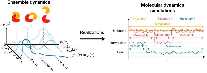
Figure 1: Illustration of the relationship between the ensemble view of dynamics and the individual realizations we obtain from molecular dynamics simulations.

2 Strategies for MSM estimation, validation, and analysis

As we saw above, building MSMs relies on discretizing conformational space into N disjoint segments. These segments need to provide a good basis for approximating the Propagator Eigenfunctions to ensure we achieve the best possible approximation of the full space dynamics’. The dimensions of the continuous space dynamics are many, for all but the simplest system, so it is not practical to place a fine grid on all dimensions. Placing such a grid would require enormous computer memory and simulation data to be successful. We are facing what in statistics is called the curse of dimensionality. In practice, building a MSM involves a sequence of four steps [32],

• Featurization – selecting a suitable representation of the molecular system

• Dimension reduction – reducing the representation of the molecular system

• Clustering – discretization of the representation

• Transition matrix estimation – estimation of the MSM,

each of these steps naturally introduces a substantial number of possible modeling decisions. The following sections outline successful principles to enable effective decision-making for all these steps.

Variational approach for conformational dynamics and Markov processes (VAC and VAMP)

When we build MSMs, we express the molecules’ thermodynamic and kinetic properties on a discrete set of disjoint states. Adopting this strategy means that we approximate the eigenfunctions using a combination of indicator functions – functions that return one if we in a certain area of configuration space and zero everywhere else. However, this is just one way of approximating the Eigenfunction, and we are free to approximate them with any function we like. The variational approach for conformational dynamics (VAC) [53, 54] gives us a principle to select the function that best approximates a molecular system’s slow dynamics from a set of trial functions. Here, I briefly outline the idea – more detailed treatments are available elsewhere.

VAC uses that the Eigenvalues of $\mathcal{P}_{\tau}$ are bounded and the Eigenfunctions form an orthonormal basis. Consequently, if $f_{\alpha}$ is an approximation of the $\alpha$’th Eigenfunction of $\mathcal{P}_{\tau}$ the auto-correlation is given by

$$c_{\tau}(f_{\alpha})=\int f_{\alpha}(x)\mu^{-1}(x)\mathcal{P}_{\tau}f_{\alpha}(x)\,\mathrm{d}x\leq\lambda_{\alpha}$$

where the equality holds if and only if $f_{\alpha}(x)$ is exactly the $\alpha$’th Eigenfunction of $\mathcal{P}_{\tau}$. Hence the variational principle tells us that we will always approximate the auto-correlation of an exact Eigenfunction $\phi_{\alpha}(x)$ from below. Practically, this means we can devise algorithms to approximate a set of orthonormal approximations of the Eigenfunctions of $\mathcal{P}_{\tau}$.

A more general Variational approach for Markov processes (VAMP) [55], extends VAC to non-reversible dynamics, non-equilibrium data, and allows us to define scores which can be used for hyper-parameter optimization, cross-validation, and model selection when building MSMs. These VAMP-scores summarize the auto-correlations on a set of basis functions (features), which best approximate the underlying dynamics, and therefore how well they represent slow dynamics. We can use the VAMP-scores at every step of the MSM building process to evaluate how well our modeling decisions will allow us to represent the slow dynamics of a molecular system.

Feature selection

To facilitate the estimation of MSMs, we will need to arrive in a sufficiently low-dimensional space to allow effective discretization. However, the space has to include sufficient detail to capture the interesting slow processes in our dataset. Fortunately, we frequently have a clear idea of what kinds of processes we are interested in resolving, or more specifically, what features we are not interested in resolving. For example, in many cases, we are not directly interested in studying the influence of solvation or the rotational and translational motion of the solutes. This focus leaves us with studying different internal coordinates or inter-molecular coordinates when selecting features for building MSMs. These internal coordinates – or features – typically include contacts, distances, angles, and torsions between atoms or atom groups.

While the considerations outlined above refines our choice of possible structural features to use in our model building, it still leaves open an enormous set of potential structural features. To further narrow down this ambiguity, there are two different strategies:

1. Manual feature selection by selecting features based on chemical, biological, or physical insights which give us some information about possible slow processes

2. Algorithmic feature selection strategies.

It is difficult to approach the first strategy in a general and systematic way. Typically, this strategy involves manually refining the selection of features such that the model is robust and provides the necessary predictive and descriptive power envisaged for the project. The second approach is typically more systematic and generalizable and will normally be the best choice if we know little about the system beforehand. Several methods provide automated feature selection specifically designed with MSM building in mind: Scherer, Husic et al. illustrate use of VAMP in this respect [56], and Chen et al. use a genetic algorithm based method for feature selection [57]. The former method works directly on the features, whether the latter approach relies sub-sequent modeling steps to evaluate the selected features. Therefore, the latter method is susceptible to confounding factors limiting when evaluating the quality of a set of features.

Dimensionality Reduction

Usually, pre-selecting several features (distances/contacts, angles, features etc) using the strategies outlined above is insufficient to sufficiently reduce the space to enable effective discretization of the conformational space. Alternatively, we may not know much about the system before starting our analysis, and we may want to identify structural features that characterize the molecular dynamics well. To face this problem, we can use dimensionality reduction techniques. These methods remove dependencies in the input data through linear (or non-linear) combinations learned utilizing a range of different optimality criteria, thereby allowing us to represent the original data in a lower-dimensional space while keeping the optimality criteria used as small as possible. Dimensionality reduction techniques have their origin in machine learning and statistics in a branch which is now broadly referred to as unsupervised learning.

In the context of MSM, principal component analysis (PCA) [58, 59, 60, 61] and time-lagged independent component analysis (TICA) [62, 63, 64] are the most widely used, limiting the discussion here to these two.

PCA seeks to define a linear projection,

$$\mathbf{Y}=\mathbf{X}\mathbf{W}$$

of the set of input features, $\mathbf{X}\in\mathbb{R}^{N_{\mathrm{numframes}}\times N_{\mathrm{numfeats}}}$, to maximize the variance of each of the dimensions of $\mathbf{Y}\in\mathbb{R}^{N_{\mathrm{numframes}}\times N_{\mathrm{reduceddim}}}$, by learning $\mathbf{W}\in\mathbb{R}^{N_{\mathrm{numfeats}}\times N_{\mathrm{reduceddim}}}$, subject to an orthonormality constraint on the columns of $\mathbf{W}$ to ensure each dimension in $\mathbf{Y}$ is uncorrelated and normalized. Consequently, PCA gives us a new set of features that best capture our input features’ variance and is an appropriate choice if we are interested in studying processes characterized by large-scale structural fluctuations.

TICA similarly seeks to find a linear projection as for PCA. However, instead of maximizing the variance, TICA uses the variational principle of conformational dynamics to determine projections with the slowest auto-correlation. Consequently, TICA is the appropriate choice if slow motions are of interest when studying a molecular system. Recall, slow dynamics is what consititute the dominating part of the propagator. Practically, we compute TICA by solving the generalized Eigenvalue equation (subject to appropriate normalizations),

$$\mathbb{C}_{\tau}\mathbf{w}_{i}=\mathbb{C}_{0}\lambda_{i,\tau}\mathbf{w}_{i}$$

where $\mathbb{C}_{\tau}=\frac{1}{N_{\mathrm{numframes}}-\tau}\mathbf{X_{:\mathrm{numframes}-\tau}^{\top}}\mathbf{X}_{\tau:}$ and $\mathbb{C}_{0}=\frac{1}{N_{\mathrm{numframes}}}\mathbf{X^{\top}}\mathbf{X}$ are the time-lagged and instantenous covariance matrices, respectively. $\mathbb{C}_{\tau}$ computes the covariance between features spaced in time by $\tau$, and the indices $:\mathrm{numframes}-\tau$ and $\tau:$ mean all but the last $\tau$ frames and the all but the first $\tau$ frames, respectively. At this point $\tau$ is an integer with a time-unit of the spacing interval between the frames in your MD trajectory data. We can use the independent components, $\mathbf{w}_{i}$, which solve this equation and correspond to the largest eigenvalues $|\lambda_{i,\tau}|<1$ to project the data on to a lower-dimensional space, $\mathbf{y}_{i}=\mathbf{X}\mathbf{w}_{i}$, which conserve the slowest dynamic modes in the system. We use the total kinetic variance $\varsigma_{\tau}^{2}$ to quantify how much dynamic is preserved in the $d$-dimensional projection ($d<N_{\mathrm{numfeats}}$),

$$\varsigma_{\tau}^{2}=\frac{\sum_{i=2}^{d}\lambda_{i,\tau}^{2}}{\sum_{j=2}^{N_{\mathrm{numfeats}}}\lambda_{j,\tau}^{2}}.$$

Both PCA- and TICA-based dimension reduction methods are part of the major MSM software packaged PyEMMA [65, 32] and MSMBuilder [66].

Recent surveys discuss the use of non-linear dimensionality reduction techniques in the context of MSM estimation. While promising, these methods have not seen broad adoption so far.

Clustering

MSMs rely on discretizing the configurational space into disjoint configurational states – micro-states. Clustering is the step where the grouping of molecular configurations into discrete states happens. The most commonly applied algorithm towards this purpose is $k$-means clustering, yet several other methods perform this task with a variety of different strategies [67]. As for feature selection, we can use VAMP scores and cross-validation to evaluate our clustering quality. Below, I expand on other considerations which are important when clustering states when studying protein-protein encounters.

Model Estimation and Validation

Following clustering, we can assign every molecular configuration to a Markov state. Trajectories now realize a jump-process on a set of, $N$, discrete states, each of the states are connected back to a molecular configuration. We call these discrete trajectories, $D=\{d_{1},\dots,d_{M}\}$. The task of estimating a Markov state model corresponds to computing the most likely transition probabilities, $t_{ij,\tau}$ between any two states $i$ and $j$ after a lag-time of $\tau$. Recall, we assume the dynamics are Markovian, so the likelihood of observing our data, $D$, is equal to the product of all the transition probabilities,

$$\ell(T_{\tau}\mid D) = \prod_{d\in D}p(d[\tau]\mid d[0],\tau)p(d[2\tau]\mid d[\tau],\tau)\dots p(d[M]\mid d[M-\tau],\tau)$$

$$= \prod_{d\in D}t_{d[0]d[\tau],\tau}t_{d[\tau]d[2\tau],\tau}\dots t_{d[M-\tau]d[M],\tau}$$

$$= \prod_{ij}t_{ij,\tau}^{C(\tau)_{ij}}$$

$C(\tau)$ is the count matrix where each element $C(\tau)_{ij}$ is the number of transitions between states $i$ and $j$, with a time-lag, $\tau$, observed in all the trajectories, $D$. Estimating a MSM then corresponds to finding the transition probabilities, given the observed transition counts in the count matrix, $C(\tau)$. We can either do maximum likelihood estimation[68, 30], or Bayesian posterior sampling of the transition probabilties [69, 36]. The first approach gives us the one most likely model whereas the latter approach gives us a distribution of models which we can use to compute properties as well as their uncertainties.

Major MSM software packages implement algorithms to perform inference via either mode, with options to enforce constraints such as detailed balance [36, 69] or a fixed stationary distribution [70]. As outlined above, the detailed balance constraint ensures a reversible MSM is estimated and reduces the number of degrees of freedom to be estimated. Adding constraints to the estimation when possible is often desirable, as it may increases robustness of the results.

Choosing the lag-time when building a MSM decides the effective time-resolution of the resulting model [71]. Consequently, we want to keep this number small, too preserve as much of the information in our data as possible. However, since we reduce a high-dimensional space down to a lower-dimensional one to enable discretization, there is no guarantee that the projected dynamics will be Markovian at short lag-times [72, 73, 74]. We check the ’Markovianity’ of the projected dynamics by computing the ITS as a function of lag-time and ensuring no systematic change in the ITS as a function of lag-time considering the statistical uncertainty. A good choice of lag-time is then one which as short as possible, yet shows now significant change in the ITS when increased or decreased slightly. This analysis is typically facilitated by an ITS plot, showing the ITS as a function of lag-time.

Having selected an appropriate lag-time, we can test the resulting MSM for self-consistency with the simulation data via the Chapman-Kolmogorov (CK) test [30, 20]. This test makes use of the time-discrete Chapman-Kolmogorov equation

$$T_{k\tau}=T_{\tau}^{k}$$

which predicts that the transition probabilities of a model estimated with lag-time $k\tau$ should be equal to the transition probabilities of a model estimated with lag-time $\tau$ to the power of $k$. We typically visualize the CK test by comparing the values on either side of the equation with error bars as a function of integer multiples of the MSM lag-time. As for the ITS analysis, we here aim to see agreement within statistical uncertainty. Usually, only a reduced set of states, or a coarse-grained model, is used to facilitate analysis.

Spectral gaps and Coarse-graining

It is not uncommon that MSMs end up having hundreds or thousands of micro-states. The large number of micro-states helps us bring down the error when approximating Eigenfunctions. However, it can stifle the subsequent analysis. Consequently, we often coarse-grain the MSMs into a handful of meta-stable macro-states, which summarize the slow dynamics. Coarse-graining here should not be confused with coarse-grained simulations, where beads represent multiple atoms. We have to decide how many states, and that number may not be evident from the start. In many cases, we can use the spectral gap in the Eigenvalue spectrum of the MSM to decide on how many states we need to coarse-grain a MSM to, to ensure we represent the slow dynamics.

Suppose we sort the Eigenvalues-Eigenvectors pairs of a MSM by the amplitude of the Eigenvalue, and plot them. In that case, we often see one or more drops in the amplitude with increasing index (decreasing Eigenvalue). These drops are spectral gaps and pin-point separations between fast and slow dynamics in the molecular system represented by the MSM. We can use these spectral gaps to decide on how many states to use for a coarse-graining, as every Eigenfunction specifies what two regions of conformation space are exchaning on the ITS which can be computed from the Eigenvalue. Consequently, if we have $n$ Eigenvalues which are less than 1 above a spectral gap, a $n+1$ state coarse-graining will be appropriate.

Perron Cluster-Cluster Analysis (PCCA) [75, 76] is a method that groups together micro-states based on the structure of the Eigenvectors of a MSM is the most common way to identify important meta-stable macro-states sampled during molecular dynamics simulations. Two related algorithms, PCCA+ and PCCA++, find an optimal linear transformation of the Eigenvector coordinates onto a probability simplex [77].

Hidden Markov state models (HMM) are an alternative to both MSMs and PCCA [78]. HMMs avoid the assumption of MSMs of Markovian dynamics in the reduced space by estimating a “hidden” Markov chain observed indirectly via the trajectory data on the discrete micro-states. A HMM therefore estimates a transition probability matrix, and an “emission matrix,” $E$, the first matrix is responsible for modeling the dynamics, and the latter models the observation process: given we are in hidden state $i$ we will be in microstate $j$ with probability $p(j\mid i)=E_{ij}$. Consequently, the emission matrix tells us what states exchange rapidly, given we are in a specific meta-stable configuration. We can use this to simplify the many states into just a few states. HMMs have a range of other theoretical advantages but are also more challenging to estimate than MSMs. There are other alternatives to defining lower-dimensional models to facilitate analysis of slow dynamics in terms of a few meta-stable states. However, their performance in the context of protein-protein encounters is currently unknown [79, 80].

Adaptive and enhanced sampling strategies

The quality of the molecular dynamics simulation data ultimately determines the quality of the estimated MSMs. Here, quality means the number of transitions sampled between configurational states of interest for the molecular system. An advantage of MSM analysis is that we do not necessarily need to sample transitions between all states of interest in every trajectory but sample only a subset of the possible transitions. However, in practical cases, we still have to make the most of limited resources – blindly or naively running numerous simulations may not be the most effective.

Adaptive sampling strategies (semi) automatically decide how multiple simulations run in parallel and over several “epochs.” These strategies have to balance exploration and exploitation: sampling new states and refining sampling statistics between previously visited states [81, 82, 83]. Several groups have proposed strategies using different assumptions about what is important to characterize molecular systems [81, 27, 47, 84, 85, 86, 87, 88]. A complementary set of strategies aim to sample transitions between known states [89, 90, 91]. However, due to the relatively high computational cost of studying protein-protein encounters, these methods are yet to be compared in rigorous benchmarks.

Enhanced sampling methods bias molecular dynamics simulations intending to speed up sampling processes of interest, such as protein-protein binding and unbinding [92, 39, 38, 37, 93]. Unfortunately, introducing the right biases to enhance the sampling of a process of interest remains a labor-intensive process. Nevertheless, methods are available to recover stationary properties from biased simulations, yet proving more difficult for dynamic properties. However, combining unbiased and biased simulation data via recent MSM estimation techniques can significantly improve the estimated models’ robustness [94, 95, 96, 97, 98, 29]. In section 4 we highlight the successful use of adaptive and enhanced sampling techniques to study protein-protein binding-unbinding modeling.

Practical consideration for studying protein-protein encounters

The procedures outlined above generally apply to molecular systems. However, there are additional aspects that are critical to be mindful of when modeling protein-protein encounters.

We can use macroscopic variables, including concentration, temperature, pressure, and mutations, to control the molecular system’s ensemble, including the population of bound and unbound states and their kinetics of exchange. As we have discussed, following experimental observables as a function, these variables allow us to quantify essential properties such as affinities, rate constants, and structural information about the complex formation process.

Computationally, we often have to settle on a single – or a few – macroscopic setting(s) of variables to study. This limitation is due to the large computational requirements associated with sampling each condition, even using the advanced simulation strategies, including those outlined above. A notable exception is the temperature, which is leveraged in enhanced sampling techniques to improve sampling efficiency. When analyzed together with regular MD simulation data using appropriate statistical estimators, they may improve MSM estimation. However, using these data on their own makes it challenging to get insights about exchange kinetics between conformational states.

The primary differences we face when studying protein-protein encounters, compared with studying the molecular dynamics in a single protein molecule, are stoichiometry and concentration. Practically, the simulation volume is limiting: when we increase the volume, we need to simulate larger systems, usually comprised of an increasing number of water molecules. This fact makes simulations with high protein concentrations the only computational viable strategy currently.

A high concentration in molecular dynamics has some practical consequences which may make it practically difficult to study certain mechanisms of protein-protein encounters. Let us consider a case of the conformational selection mechanism, where a low-population state $A^{*}$ of unbound protein $A$ binds the protein $B$ to form the complex $A^{*}:B$ in the following reversible chemical kinetic relation

$$A\rightleftarrows A^{*}+B\rightleftarrows A^{*}:B$$

where $k_{A\rightarrow A^{*}}\ll k_{A^{*}\rightarrow A}$ with both rates being independent of concentration. We assume the protein $B$ does not undergo conformational changes which perturb this relation directly. The on-rate, $k_{A^{*}+B\rightarrow A^{*}:B}$, is proportional to the protein concentration and the population of the unbound state of $A^{*}$, so as concentrations increase, the probability of observing binding events increase. In an alternative binding mechanism (induced fit) binding happens before conformational change in the protein $A$,

$$A+B\rightleftarrows A^{*}:B.$$

Here, the on-rate (the rate of binding), $k_{A+B\rightarrow A^{*}:B}$, depends on the protein concentration and the population of the highly populated state of protein $A$. In many reported cases both mechanisms are possible, consequently, we seek to understand the balance of these two mechanisms – more generally, we seek to characterize the association-dissociation path ensemble [99, 100]. However, since we are at high concentrations we may have $k_{A^{*}+B\rightarrow A^{*}:B}\ll k_{A+B\rightarrow A^{*}:B}$, and we may even have $k_{A\rightarrow A^{*}}\ll k_{A^{*}\rightarrow A}\ll k_{A+B\rightarrow A^{*}:B}$. So with only finite MD simulation data, we may severely under-sample or completely miss certain mechanisms, even if they are important. In other words, high protein concentrations in MD simulations may increase the free energy of the unbound state to the point where the association is barrier free, and the unbound state is not meta-stable [8].

More concretely, given the competition between these mechanisms, sampling the induced-fit mechanism is much more likely than sampling the conformational selection mechanism. Even conformational sampling of protein $A$ is much less likely than sampling binding via induced fit. Practically, these conditions mean that we will have an intrinsic preference to observe a certain biophysical binding mechanism and may over-sample mechanisms that are not relevant at physiological protein concentrations, including unspecific binding events. As a result, we would need to acquire more simulation data to ensure statistically sufficient sampling of alternative binding mechanisms and conformational mixing of the unbound states.

The fast on-rates at high concentrations may also influence our ability to distinguish unbound and bound states automatically. The time-scale, $t_{i}$, of a process, $i$, between states $a_{i}$ and $b_{i}$ is depends on the geometric average of the rates of the forward and backward process $t_{i}=\frac{1}{\kappa_{i}}=\frac{1}{k_{a_{i}\rightarrow b_{i}}+k_{a_{i}\rightarrow b_{i}}}$, which is numerically dominated by the faster (larger) rate. As a result, the binding-unbinding process’s time-scale will be fast. Therefore, dimension reduction techniques may not resolve it as an important process. Consequently, a MSM based on a clustering defined only in this space will miss the process altogether. However, we can overcome this problem by explicitly separating bound and unbound states, such as a molecular feature that clearly distinguishes the unbound and bound states.

The chosen forcefield model may significantly affect the sampled binding mechanisms and may be prone to deficiencies such as strong unspecific binding. Although efforts continuously improve these forcefield models address their outstanding limitations, we often do not know how well it will represent a new system of interest before we start simulations. In the next section, we discuss strategies to validate MSMs built using potentially imperfect forcefield models and possibly overcome some of the limitations.

Analysis of the association-dissociation path ensemble

The ’mechanism’ of binding is ultimately governed by the statistical distribution of different paths from the unbound state to the bound state. The importance of the different paths between the unbound and bound states is governed by the flux along that path. Transition path theory (TPT) [99, 100, 35, 20] provides us with a theoretical framework through which we can compute reactive flux-matrices from MSMs of protein-protein encounters. The ’reaction’ here refers to the transition from a set of ’reactant states’ (unbound) $A$ to a set of ’product states’ $B$ (bound). TPT gives us tools to assign all intermediate states $I$ (not bound, and not unbound), committor probabilities, $q^{+}$ and $q^{-}$, which tells gives us the probability of reaching the $B$ before $A$ from an intermediate state $i\in I$ via forward committor $q_{i}^{+}$ and vice-versa for the backward committor $q_{i}^{-}$. We can further use this framework to compute mean first passage times (MFPT), for example the average on- and off-rates, as well as dissect all the possible pathways from unbound to bound states. TPT is therefore an important tool for analysis of MSMs, in particularly when we want to understanding a specific process. Major MSM softwares implement TPT analyses and plotting functions to visualize the results [32, 65, 66].

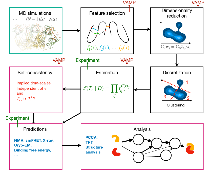
Figure 2: Flow-chart of Markov state modeling from molecular dynamics simulations to final model and analysis. Boxes are colored to indicate data collection (cyan), data processing and model estimation (black), and analysis and validation (magenta). I highlight steps which may benefit from specific techniques or experimental data with colored pins.

3 The connection to experiments

In favorable cases, appropriately validated MSMs predict molecular mechanisms with high temporal and spatial resolution. These insights can, of course, guide our understanding of important molecular phenomena associated with, for instance, protein-protein binding. However, so far, we have only discussed validation as statistical self-consistency and minimizing projection errors (optimizing variational scores). Since we generate the simulation data that we use to drive the estimation MSMs with imperfect classical empirical force field models, agreement with experimental data is not a given. In this section, I will outline how we can predict important biophysical observables to check for agreements, the limitations of these comparisons, and how we may integrate experimental data into the estimation of MSMs using the Augmented Markov model framework, to bring experiment and simulation into alignment.

3.1 Experimental observability, forward models, and errors.

What is an observable? – In our context, an experimental observable is a function of state; that means a function of the configurations adopted by a molecular system at specific experimental conditions. The definition encompasses both bulk experiments, where a very large number ($\sim 10^{23})$ of copies of identical systems cumulative signal is measured, and experiments where time-resolved trajectory signals from single molecules are measured. The manifestation of a particular observable is described by a physical model, $f(\cdot)$, describing the relationship between a configuration of the system, $x$, and the observed signal, $o$. Simple examples of $f$ may be a ruler measuring the Euclidean distance between two atoms in a molecule, or a function computing the potential energy of the system configuration, $x$.

In a stationary bulk experiment at equilibrium we measure an expectation value of $f(\cdot)$ under the Boltzmann distribution,

$$\langle O_{f}\rangle = \mathcal{Z}^{-1}\int f(x)\exp(-\beta U(x))\,\mathrm{d}x$$

$$= \int f(x)\mu(x)\,\mathrm{d}x$$

$$= \mathbb{E}_{\mu(x)}[f(x)].$$

We use $p(x)$ as short-hand for the normalized Boltzmann distribution for a given $\beta$, and the brakets to denote ensemble averages.

In an ergodic, dynamic bulk experiments at equilibrium we measure the auto-correlation,

$$\langle O_{f}(0)O_{f}(\Delta t)\rangle = \int\int f(x^{\prime})p(x^{\prime}\mid x;\Delta t)p(x)f(x)\,\mathrm{d}x\mathrm{d}x^{\prime}$$

$$= \mathbb{E}_{p(x)}[\mathbb{E}_{p(x^{\prime}\mid x,\tau)}[f(x^{\prime})f(x)]]$$

where $p(x^{\prime}\mid x;\Delta t)$ is the transition probability. Note that we may analogously define cross-correlation experiments by using two different models for the observables,

$$\langle O_{f_{a}}(0)O_{f_{b}}(\Delta t)\rangle = \mathbb{E}_{p(x)}[\mathbb{E}_{p(x^{\prime}\mid x,\tau)}[f_{b}(x^{\prime})f_{a}(x)]].$$

Some experimental setups will allow us to initialize an ensemble in a non-equilibrium ensemble $p_{0}$ and follow the relaxation process back to equilibrium [35, 20]. Such experiments include pressure- and temperature-jump, as well as, stopped-flow. Cross-correlation functions measured in such relaxation experiments can be expressed as,

$$\langle O_{f_{a}}(0)O_{f_{b}}(\Delta t)\rangle_{p_{0}} = \int\int f_{b}(x^{\prime})p(x^{\prime}\mid x;\Delta t)\frac{p_{0}(x)}{p(x)}f_{a}(x)\,\mathrm{d}x^{\prime}\mathrm{d}x.$$

In single molecule experiments observables are followed over time as trajectories, with some time resolution $\Delta t$, in its simplest form:

$$O_{f}=\{f(x(0)),f(x(\Delta t)),\dots,f(x(N\Delta t))\}.$$

Sources of errors and uncertainty

In a typical setting, we have some set of experimental data, which may include any combination of the classes above, and we wish to compare these observables to corresponding predictions made by our computational model stationary and dynamic properties of the molecular system. Several sources of uncertainty and error may arise in this setting that we will have to be mindful of:

1. Experimental noise (thermal noise, shot-noise, etc.)
   This category includes every stochastic noise contribution due to limitations in the experimental setup, typically due to imperfections in instrumentation measurements or sample (labeling) stability. In many cases, theoretical analyses of experiments are available which may help decide how this error should be modeled.

2. Systematic experimental errors/biases
   These errors and biases arise due to imperfect referencing — in the case of for example relative experimental measurements — or unknown, or imprecise, experimental conditions (temperature, concentrations, pressure, etc) or fluctuations of these parameters during data acquisition. This source of error is typically more challenging to systematically model or perfectly compensate for and often require substantial knowledge of the experimental setup.

3. Systematic error in the computational model of the molecular system dynamics
   Computational models of $p(x)$ and $p(x^{\prime}\mid x,\Delta t)$ are typically estimated using finite simulation data using from empirical forcefield models. The quantitative agreement of these with experiment is ever improving, however, still suffer significant systematic errors. The errors may arise from the classical approximations made of quantum mechanical interactions, to make simulations computationally tractable, or other approximations. Our efforts to compare simulation models to experiments are typically driven by the recognition of these issues, and a desire to understand the limitations and merits of a given moded. Another systematic error encompassed in this section is the sampling error, where we simply do not have enough simulation data to accurately estimate $p(x)$ and $p(x^{\prime}\mid x,\Delta t)$.

4. Modeling error of observable functions $f(\cdot)$
   Like simulation models, the forward prediction of instantaneous (time-independent) experimental observables approximate complicated experimental setups or quantum mechanical phenomena in a computationally efficient manner. In many cases, quantifying errors and biases in these models is challenging.

3.2 Predicting experimental observables using MSMs

The expressions given above for the experimental observables are general for any ergodic, Markovian dynamics, at, or relaxing to, a time-invariant equilibrium state. However, for molecular systems, these expressions involve intractable integrals over the configuration space. Fortunately, for MSMs, these integrals simplify to standard linear algebra operations, which we can compute efficiently.

The discretization of configurational space, $\mathcal{S}=\{S_{1},\dots,S_{N}\}$, associated with the MSM, leads to a discretization of the instantaneous experimental observable (predicted via $f(\cdot)$) as the vector $\mathbf{a}\in\mathbb{R}^{N}$, with elements,

$$a_{i}=\text{$\frac{1}{\int_{x\in S_{i}}p(x)\,\mathrm{d}x}$}\int_{x\in S_{i}}p(x)f_{a}(x)\,\mathrm{d}x\approx\frac{1}{N_{S_{i}}}\sum_{j\in S_{i}}f(x_{j})$$

where $S_{i}$ is configurational space segment, or its finite sample approximation with $N_{S_{i}}$ samples. We can extend this expression to vector-valued observables. Since this discretization replaces a function which takes on arbitrary real valued numbers for different conformations, by a piece-wise constant function, we hope to minimize the variance of $f(x)$ within each $S_{i}$ to ensure a good approximation.

We use the stationary distribution $\pi$, of the transition matrix $T_{\tau}$, along with discretized feature vector $\mathbf{a}$ to compute stationary bulk experimental observables as,

$$\langle O_{f_{a}}\rangle=\pi\cdot\mathbf{a}=\sum_{i=1}^{N}\pi_{i}a_{i}.$$

The expression for dynamic bulk experiments, can be expressed using the transition matrix,

$$\langle O_{f}(0)O_{f}(N\tau)\rangle = \mathbf{a}^{\top}\boldsymbol{\Pi}T(\tau)^{N}\mathbf{a}$$

where $\boldsymbol{\Pi}=\text{diag}(\pi)$ is a matrix with stationary probabilities on the diagonal, and zeros elsewhere. $N$ is an integer expressing time in multiples of the MSM lag-time $\tau$. Cross-correlation experiments can similarly be expressed a

$$\langle O_{f_{a}}(0)O_{f_{b}}(N\tau)\rangle=\mathbf{b}^{\top}\boldsymbol{\Pi}T(\tau)^{N}\mathbf{a}$$

where $\mathbf{b}$ is defined as $\mathbf{a}$, but for a observable predicted by $f_{b}(\cdot)$. In general, MSMs predict auto- and cross-correlation function as mixture of exponential decays. We see this more directly by considering the spectral decomposition of the transition matrix,

$$\langle O_{f}(0)O_{f}(N\tau)\rangle = \mathbf{a}^{\top}\boldsymbol{\Pi}\left(\sum_{i=1}^{N}\lambda_{i}^{N}\boldsymbol{l}_{i}^{\top}\mathbf{r}_{i}\right)\mathbf{a}$$

$$= \sum_{i=1}^{N}\lambda_{i}^{N}(\mathbf{a}^{\top}\cdot\boldsymbol{l}_{i}^{\top})(\boldsymbol{l}_{i}\cdot\mathbf{a})$$

$$= \sum_{i=1}^{N}\exp(-\frac{N\tau}{t_{i}})(\boldsymbol{l}_{i}\cdot\mathbf{a})^{2}$$

$$= (\pi\cdot\mathbf{a})^{2}+\sum_{i=2}^{N}(\boldsymbol{l}_{i}\cdot\mathbf{a})^{2}\exp(-\frac{N\tau}{t_{i}}).$$

Similar expression can be written down for cross-correlation and relaxation experiments (Keller Prinz fingerprints). This simple form of the auto- and cross-correlation functions from MSMs facilitates analytical expression of several experimental observables including from NMR spectroscopy, dynamic neutron scattering, and FRET spectroscopy.

3.3 Integrating experimental and simulation data into Augmented Markov models

As mentioned above, systematic errors in the empirical force field models used for molecular simulations to build MSMs lead to statistically robust yet systematic errors in our predictions. Using the equations above, we can quantify, but not remedy, these biases. A wealth of methods have been introduced to bias MD simulations [101, 102, 103, 104, 105, 106, 107, 108], or reweight simulation data a posteriori [109, 107, 110, 111, 112, 113, 114, 115], to match experimental data, using different inference philosophies – several excellent reviews discuss these approaches in more detail [116, 117, 118]. In the context of MSMs, we already have simulation data available or are in the process of adaptively acquiring it. Consequently, adopting an approach that would alter our MD simulations’ ensemble simulations is undesirable – excluding the use of experimental data to bias simulations. On the other hand, reweighing MD trajectories generally sacrifice the dynamic information from our simulation data.

The augmented Markov models (AMM) [111] framework allows us to balance experimental and simulation data when building Markov models of molecular kinetics. AMMs therefore achieve better agreement with experimental data while preserving the dynamic information from molecular simulations. To estimate AMMs the log-likelihood function of MSMs augmented with a term to balance systematic discrepancies between experimental and simulation data via a set of Lagrange multipliers $\boldsymbol{\lambda}$,

$$\ell(T_{\tau},\boldsymbol{\lambda}\mid\mathbf{C}(\tau),\mathbf{O},\boldsymbol{\sigma})\propto\sum_{ij}c_{ij}\log t_{ij,\tau}-\sum_{k}\frac{(\hat{m}_{k}-o_{k})^{2}}{2\sigma_{k}^{2}}$$ (2)

where $t_{ij,\tau}$ is the $i,j$’th element of $T_{\tau}$, $c_{ij}$ the corresponding element in the count matrix $\mathbf{C}(\tau)$, and $o_{k}$ and $\sigma_{k}$ are the $k$’th experimental observable and its experimental uncertainty respectively. The prediction of the experimental expectation value from $T_{\tau}$ is $\hat{m}_{k}=\mathbf{a}_{k}\cdot\hat{\pi}$ with

$$\hat{\pi}_{i}=\frac{\pi_{i}\exp(\sum_{v}\lambda_{v}a_{v_{i}})}{\sum_{j}\pi_{j}\exp(\sum_{v}\lambda_{v}a_{v_{j}})}$$

models the experimental Boltzmann distribution via a Maximum Entropy perturbation of the simulation ensemble $\pi$ computed from $T_{\tau}$. $\lambda_{v}$ is the $v$’th Lagrange multiplier corresponding to experimental observable $o_{v}$ and its back-prediction for a Markov state $i$ as $a_{v_{i}}$. Optimizing (eq. 2) subject to detailed balance constraints yields an AMM.

We motivate the use of a Maximum Entropy perturbation as it provides a model as close as possible – in the Kullback-Liebler sense – to the simulation ensemble. The critical assumption is therefore that the simulation ensemble provides a reasonable starting point to model the experimental data, including covering all meta-stable configurations necessary accurately predict the experimental observables.

Other approaches similarly allow for the integration of experimental data into MSM estimation. One approach enables the gradual adjustment of MSM stationary distributions against target observables [119]. Matsunaga and Sugita present a method to integrate single-molecule FRET data and molecular simulation using a step-wise HMM estimation procedure [120]. Brotzakis et al. propose a maximum entropy and maximum caliber approach to reweigh trajectory ensembles against bulk observables [112].

Although the integration of experimental data and simulation data has been an active area of research for several decades, several problems remain open. In particular, some data still cannot be included in the AMMs framework, including single-molecule FRET trajectories or dynamic bulk observables.

4 Protein-protein and protein-peptide encounters

Several groups have reported kinetic models of protein-protein and protein-peptide encounters using molecular dynamic simulations and MSMs. As yet, tightly binding complexes (small dissociation constants, $K_{D}$) with slow association-dissociation kinetics dominate the literature, as they constitute the biggest challenge for molecular simulations. While slow macroscopic kinetics, and large free energy differences, characterize these systems, microscopically, these protein-protein and protein-peptide encounters may happen via multi-step processes. Consequently, we can sample rare events on the seconds to minutes time-scale by connecting the bound and unbound states sampling the much more likely transitions between intermediate states. MSMs excel in cases such as these: transitions sampled between intermediate steps along binding-unbinding paths can be combined into a model that predicts the slow macroscopic dynamics of the full binding-unbinding process inaccessible for direct simulation.

The first reported study of a full reversible protein-protein binding study by all-atom molecular dynamic simulations was for the inhibitory complex of ribonuclease barnase and barstar. The barnase:barstar complex is an excellent benchmark system due to its extensive experimental charaterization by multiple biophysical methods. Plattner et al. collected molecular simulations with 2 milliseconds of aggregate simulation length [27]. The data was distributed between 1.7 milliseconds of independent simulations initiated from dissociated states and 0.3 milliseconds using adaptive sampling. The adaptive scheme allowed the authors to sample barnase:barstar association with a few microseconds of aggregate simulation time, while the equilibrium binding rate is tens of microseconds. Unbinding similarly benefitted from adaptive sampling, with unbinding events being sampled in a few hundred microseconds, while the equilibrium off-rate is expected to be on the hours time-scale.The authors estimated a HMM to compute the thermodynamics, kinetics, and important structural states of the protein-protein encounter process. They compare predictions of macroscopic thermodynamics and kinetic observables against experiment: binding free-energy $12-19\,\mathrm{kcal}\cdot\mathrm{mol}^{-1}$ against the experimental $16.8\,\mathrm{kcal}\cdot\mathrm{mol}^{-1}$ and the dissociation rate $3\cdot 10^{-6}-10^{-1}$ compared to the experimental range of $8\cdot 10^{-5}-5.0\cdot 10^{\text{\textendash}4}\,\text{s}^{\text{\textendash}1}$. The large uncertainties, illustrate how MSMs and HMMs quality, accuracy, and precision for these quality critically rely on the number of binding and unbinding events sampled in the aggregate simulation data. Nevertheless, on-rate could be predicted with high accuracy and the most stable state coincided with the crystallographic structure (pdb: 1BRS). Further, perturbation theory allowed for accurate prediction of binding free-energy changes upon mutation within stastistical uncertainty. The resulting barnase:barstar HMM predicts a binding mechanism, where barstar can associate to all points of barnase’s surface, early intermediates preferably binds opposite to the native binding groove, and late intermediates states, and a ’trap’ state, bind close to the binding grove, but in non-native orientations. Later still in the process, complex passes through late intermediates into a pre-bound, loosely bound, and then finally the native bound state. The rate-limiting step is the pre-bound bound state which is stabilized by electrostatic and hydrophobic interactions between the two protein domains.

Two studies report MSMs of protein-peptide encounters involving the p53-antagonist MDM2 [29, 121]. The first study investigates one antagonistic pathway of MDM2 via its binding of the p53 transactivation domain (TAD) [121]. The study models this interaction via a TAD peptide and uses extensive, unbiased molecular dynamics simulations, as for the barnase:barstar study discussed above. The second study instead reports the binding of MDM2 to an inhibitory peptide PMI via integrating unbiased simulations and data from enhanced sampling [29]. The first study, reports MSM that predicts quantities with an accuracy comparable or worse than that observed for the barnase:barstar case above. Qualitatively accurate on-rates, yet off-rates do not agree with experiments – this is likely due to the relatively small data-set used here of 831 microseconds in aggregate length and force-field errors. Nevertheless, the authors can identify important structural states and investigate possible binding mechanisms. Their model favors an induced-fit binding mechanism, where TAD first binds MDM2 and then folds into the native complex structure.

For the second study [29], and in a follow-up study, the authors use multi-ensemble Markov models (MEMMs) to quantitatively predict binding thermodynamics and kinetics of MDM2 to the PMI peptide with high precision. MEMMs define MSMs over multiple thermodynamic states, such as those used in enhanced sampling techniques, including replica-exchange and umbrella sampling. This approach’s advantage relies on fewer simulation data (approximately 102 microseconds of Hamiltonian replica exchange and 500 microseconds of unbiased MD). This disadvantage depends on designing an effective enhanced sampling strategy for the system of interest, which may be challenging to achieve without substantial trial-and-error and extensive human intervention.

To summarize, MSMs and related kinetic modeling approaches are currently the only available strategy to gain microscopic insights into the thermodynamics and kinetics of protein-protein and protein-peptide encounters. These analyses can help us distinguish between different binding mechanisms, and combined with perturbation approaches, qualitative insights into the influence of point mutations impact the binding. However, collecting sufficient data remains a serious challenge when applying these methods in practice. At simulation rates of around 400-500 nanoseconds per day and GPU collecting millisecond sized datasets may take GPU-years to complete. New adaptive sampling strategies and the integration of experimental data and enhanced sampling simulations may help lower demands on unbiased simulations. Nevertheless, studies have focused on relatively small protein-protein and protein-ligand systems and interactions with high affinity. Further improvement in computing power, simulation, and analysis methods is needed to ensure these analyses can benefit structural biology more broadly. Finally, how these approaches will fare on low-affinity complex systems with a less clear separation of time-scales also remains to be understood.

5 Emerging technologies

As we saw above, Markov state models are emerging as an important tool in characterizing the thermodynamics and kinetics of protein-protein encounters in ideal cases, providing detailed mechanistic models at atomic resolution. We are steadily progressing towards better methods for featurization, dimension reduction, clustering, and adaptive sampling strategies; these advances contribute to minimizing the computational and labor effort needed to build high-quality MSMs. However, we remain reliant on access to state-of-the-art computing resources and, in many cases, the extensive manual intervention of highly-skilled researchers. We are further simulating increasing size scales poorly in terms of simulation efficiency and the amount of simulation data needed to build statistically sufficient models. A broad range of machine learning methods is currently emerging that directly address the challenges faced by MSMs.

Recall, the fundamental use of MSMs is to build a low-dimensional approximation of an infinite-dimensional molecular dynamics operator. This task relies on several pre-processing steps in sequential succession: featurization, dimension reduction, clustering, and model estimation. The success at each stage depends on the careful adjustment of hyper-parameters against an optimality criterion. An error or sub-optimal choice made early on in the sequence may negatively impact our final model’s quality. Yet, identifying and resolving such problems is often not straightforward and relies on extensive testing and manual intervention. With VAMPnets, Mardt et al. illustrate how we may, in principle, replace the entire sequence of pre-processing steps and the model estimation by an artificial neural network [122]. The key idea is to input all-atom coordinates into a neural network that outputs a categorical distribution representing a conformation membership to $N$ metastable states. The neural network’s optimization objective function is a VAMP score computed between pairs of simulation frames with a time-lag of $\tau$. The neural network learns the complicated function from molecular dynamics trajectories to a molecular kinetics model in a single step through this procedure. Extensions of VAMPnets are already emerging to improve data efficiency and impose further constraints on the modeled dynamics.

The number of states a molecular system may potentially adopt grows exponentially with its size. So, in addition to declining simulation rates with system size, we must sample a much larger conformational space. In other words, our simulations get slower, and we have to simulate more to ensure statistically sufficient models. The latter of these two problems arises from how we represent the meta-stable states as global configurations. Consequently, we need to explicitly account for every meta-stable state, even if differences between these states are only minor structural changes.

Dynamic graphical models (DGM) replaces the global representation of metastable states with local sub-systems [123]. These sub-systems are spatially localized and can be a side-chain rotamer or a whole protein domain. A DGM aims to encode the conformational states of all the sub-systems and how they influence each other’s evolution in time. Like MSMs, DGMs approximate the transition probability densities between all possible configurations of our sub-systems, yet without the need to enumerate them all explicitly. Their indirect representation of global configurations allows DGMs to rely on fewer parameters than MSMs, lowering simulation data demands. A recent study shows that this strategy can be very effective when modeling molecular dynamics, quantitatively predicting the thermodynamics and kinetics of molecular systems. As DGMs are generative models, we may also predict realistic meta-stable states not seen during the model’s estimation.

MSMs have come a long way. We now see this methodology’s regular application to the quantitative study of complex problems such as protein folding, protein-protein interactions, and conformational dynamics. The growing community of researchers, together with improvements in simulation methodology and hardware, is rapidly expanding the scope of systems we can address. With the advent of powerful machine learning-based we can expect to see these development accelerate further. These developments and their extensions bode well for Markovian models’ future in the quantitative study of protein-protein encounters.

6 Acknowledgements

I thank Dr. Rocío Mercado for comments and input on drafts of this chapter. This work was partially supported by the Wallenberg AI, Autonomous Systems and Software Program (WASP) funded by the Knut and Alice Wallenberg Foundation.

References

- [1] I..A. Nooren “Diversity of protein-protein interactions” In The EMBO Journal 22.14 Wiley, 2003, pp. 3486–3492 DOI: 10.1093/emboj/cdg359
- [2] M P Czech “The Nature and Regulation of the Insulin Receptor: Structure and Function” In Annual Review of Physiology 47.1 Annual Reviews, 1985, pp. 357–381 DOI: 10.1146/annurev.ph.47.030185.002041
- [3] Giovanna Zinzalla and David E Thurston “Targeting protein–protein interactions for therapeutic intervention: a challenge for the future” In Future Medicinal Chemistry 1.1 Future Science Ltd, 2009, pp. 65–93 DOI: 10.4155/fmc.09.12
- [4] Cecilia Blikstad and Ylva Ivarsson “High-throughput methods for identification of protein-protein interactions involving short linear motifs” In Cell Communication and Signaling 13.1 Springer ScienceBusiness Media LLC, 2015 DOI: 10.1186/s12964-015-0116-8
- [5] Anne-Claude Gavin et al. “Proteome survey reveals modularity of the yeast cell machinery” In Nature 440.7084 Springer ScienceBusiness Media LLC, 2006, pp. 631–636 DOI: 10.1038/nature04532
- [6] Nevan J. Krogan et al. “Global landscape of protein complexes in the yeast Saccharomyces cerevisiae” In Nature 440.7084 Springer ScienceBusiness Media LLC, 2006, pp. 637–643 DOI: 10.1038/nature04670
- [7] Kalyan S. Chakrabarti et al. “Conformational Selection in a Protein-Protein Interaction Revealed by Dynamic Pathway Analysis” In Cell Reports 14.1 Elsevier BV, 2016, pp. 32–42 DOI: 10.1016/j.celrep.2015.12.010
- [8] Thomas R. Weikl and Fabian Paul “Conformational selection in protein binding and function” In Protein Science 23.11 Wiley, 2014, pp. 1508–1518 DOI: 10.1002/pro.2539
- [9] Arthur G. Palmer “NMR Characterization of the Dynamics of Biomacromolecules” In Chemical Reviews 104.8 American Chemical Society (ACS), 2004, pp. 3623–3640 DOI: 10.1021/cr030413t
- [10] Wei Min et al. “Fluctuating Enzymes: Lessons from Single-Molecule Studies” In Accounts of Chemical Research 38.12 American Chemical Society (ACS), 2005, pp. 923–931 DOI: 10.1021/ar040133f
- [11] Joachim Frank “New Opportunities Created by Single-Particle Cryo-EM: The Mapping of Conformational Space” In Biochemistry 57.6 American Chemical Society (ACS), 2018, pp. 888–888 DOI: 10.1021/acs.biochem.8b00064
- [12] David D Boehr, Ruth Nussinov and Peter E Wright “The role of dynamic conformational ensembles in biomolecular recognition” In Nature Chemical Biology 5.11 Springer ScienceBusiness Media LLC, 2009, pp. 789–796 DOI: 10.1038/nchembio.232
- [13] Alexey Dementiev, József Dobó and Peter G.W. Gettins “Active Site Distortion Is Sufficient for Proteinase Inhibition by Serpins” In Journal of Biological Chemistry 281.6 Elsevier BV, 2006, pp. 3452–3457 DOI: 10.1074/jbc.m510564200
- [14] James A. Huntington, Randy J. Read and Robin W. Carrell “Structure of a serpin–protease complex shows inhibition by deformation” In Nature 407.6806 Springer ScienceBusiness Media LLC, 2000, pp. 923–926 DOI: 10.1038/35038119
- [15] Eunkyung Kim et al. “A single-molecule dissection of ligand binding to a protein with intrinsic dynamics” In Nature Chemical Biology 9.5 Springer ScienceBusiness Media LLC, 2013, pp. 313–318 DOI: 10.1038/nchembio.1213
- [16] Kenji Sugase, H. Dyson and Peter E. Wright “Mechanism of coupled folding and binding of an intrinsically disordered protein” In Nature 447.7147 Springer ScienceBusiness Media LLC, 2007, pp. 1021–1025 DOI: 10.1038/nature05858
- [17] Irina Bezsonova et al. “Interactions between the Three CIN85 SH3 Domains and Ubiquitin: Implications for CIN85 Ubiquitination†” In Biochemistry 47.34 American Chemical Society (ACS), 2008, pp. 8937–8949 DOI: 10.1021/bi800439t
- [18] Jeffrey A. Purslow, Balabhadra Khatiwada, Marvin J. Bayro and Vincenzo Venditti “NMR Methods for Structural Characterization of Protein-Protein Complexes” In Frontiers in Molecular Biosciences 7 Frontiers Media SA, 2020 DOI: 10.3389/fmolb.2020.00009
- [19] Lluís Raich et al. “Discovery of a hidden transient state in all bromodomain families” In Proceedings of the National Academy of Sciences 118.4 Proceedings of the National Academy of Sciences, 2021, pp. e2017427118 DOI: 10.1073/pnas.2017427118
- [20] Frank Noé et al. “Constructing the equilibrium ensemble of folding pathways from short off-equilibrium simulations” In Proceedings of the National Academy of Sciences 106.45 Proceedings of the National Academy of Sciences, 2009, pp. 19011–19016 DOI: 10.1073/pnas.0905466106
- [21] Emilia P. Barros et al. “Markov state models and NMR uncover an overlooked allosteric loop in p53” In Chemical Science 12.5 Royal Society of Chemistry (RSC), 2021, pp. 1891–1900 DOI: 10.1039/d0sc05053a
- [22] K. Lindorff-Larsen, S. Piana, R.. Dror and D.. Shaw “How Fast-Folding Proteins Fold” In Science 334.6055 American Association for the Advancement of Science (AAAS), 2011, pp. 517–520 DOI: 10.1126/science.1208351
- [23] D.. Shaw et al. “Atomic-Level Characterization of the Structural Dynamics of Proteins” In Science 330.6002 American Association for the Advancement of Science (AAAS), 2010, pp. 341–346 DOI: 10.1126/science.1187409
- [24] Lukas S Stelzl et al. “Local frustration determines loop opening during the catalytic cycle of an oxidoreductase” In eLife 9 eLife Sciences Publications, Ltd, 2020 DOI: 10.7554/elife.54661
- [25] Fabio Pietrucci, Fabrizio Marinelli, Paolo Carloni and Alessandro Laio “Substrate Binding Mechanism of HIV-1 Protease from Explicit-Solvent Atomistic Simulations” In Journal of the American Chemical Society 131.33 American Chemical Society (ACS), 2009, pp. 11811–11818 DOI: 10.1021/ja903045y
- [26] Nathaniel Stanley, Santiago Esteban-Martín and Gianni De Fabritiis “Kinetic modulation of a disordered protein domain by phosphorylation” In Nature Communications 5.1 Springer ScienceBusiness Media LLC, 2014 DOI: 10.1038/ncomms6272
- [27] Nuria Plattner, Stefan Doerr, Gianni De Fabritiis and Frank Noé “Complete protein–protein association kinetics in atomic detail revealed by molecular dynamics simulations and Markov modelling” In Nature Chemistry 9.10 Springer ScienceBusiness Media LLC, 2017, pp. 1005–1011 DOI: 10.1038/nchem.2785
- [28] Albert C. Pan et al. “Atomic-level characterization of protein–protein association” In Proceedings of the National Academy of Sciences 116.10 Proceedings of the National Academy of Sciences, 2019, pp. 4244–4249 DOI: 10.1073/pnas.1815431116
- [29] Fabian Paul et al. “Protein-peptide association kinetics beyond the seconds timescale from atomistic simulations” In Nature Communications 8.1 Springer ScienceBusiness Media LLC, 2017 DOI: 10.1038/s41467-017-01163-6
- [30] Jan-Hendrik Prinz et al. “Markov models of molecular kinetics: Generation and validation” In The Journal of Chemical Physics 134.17 AIP Publishing, 2011, pp. 174105 DOI: 10.1063/1.3565032
- [31] Brooke E. Husic and Vijay S. Pande “Markov State Models: From an Art to a Science” In Journal of the American Chemical Society 140.7 American Chemical Society (ACS), 2018, pp. 2386–2396 DOI: 10.1021/jacs.7b12191
- [32] Christoph Wehmeyer et al. “Introduction to Markov state modeling with the PyEMMA software [Article v1.0]” In Living Journal of Computational Molecular Science 1.1 University of Colorado at Boulder, 2019 DOI: 10.33011/livecoms.1.1.5965
- [33] Simon Olsson and Frank Noé “Mechanistic Models of Chemical Exchange Induced Relaxation in Protein NMR” In Journal of the American Chemical Society 139.1 American Chemical Society (ACS), 2016, pp. 200–210 DOI: 10.1021/jacs.6b09460
- [34] F. Noe et al. “Dynamical fingerprints for probing individual relaxation processes in biomolecular dynamics with simulations and kinetic experiments” In Proceedings of the National Academy of Sciences 108.12 Proceedings of the National Academy of Sciences, 2011, pp. 4822–4827 DOI: 10.1073/pnas.1004646108
- [35] Jan-Hendrik Prinz, Bettina Keller and Frank Noé “Probing molecular kinetics with Markov models: metastable states, transition pathways and spectroscopic observables” In Physical Chemistry Chemical Physics 13.38 Royal Society of Chemistry (RSC), 2011, pp. 16912 DOI: 10.1039/c1cp21258c
- [36] Frank Noé “Probability distributions of molecular observables computed from Markov models” In The Journal of Chemical Physics 128.24 AIP Publishing, 2008, pp. 244103 DOI: 10.1063/1.2916718
- [37] Thomas Huber, Andrew E. Torda and Wilfred F. Gunsteren “Local elevation: A method for improving the searching properties of molecular dynamics simulation” In Journal of Computer-Aided Molecular Design 8.6 Springer ScienceBusiness Media LLC, 1994, pp. 695–708 DOI: 10.1007/bf00124016
- [38] Helmut Grubmüller “Predicting slow structural transitions in macromolecular systems: Conformational flooding” In Physical Review E 52.3 American Physical Society (APS), 1995, pp. 2893–2906 DOI: 10.1103/physreve.52.2893
- [39] A. Laio and M. Parrinello “Escaping free-energy minima” In Proceedings of the National Academy of Sciences 99.20 Proceedings of the National Academy of Sciences, 2002, pp. 12562–12566 DOI: 10.1073/pnas.202427399
- [40] Mary A. Rohrdanz, Wenwei Zheng and Cecilia Clementi “Discovering Mountain Passes via Torchlight: Methods for the Definition of Reaction Coordinates and Pathways in Complex Macromolecular Reactions” In Annual Review of Physical Chemistry 64.1 Annual Reviews, 2013, pp. 295–316 DOI: 10.1146/annurev-physchem-040412-110006
- [41] Oliver F. Lange and Helmut Grubmüller “Collective Langevin dynamics of conformational motions in proteins” In The Journal of Chemical Physics 124.21 AIP Publishing, 2006, pp. 214903 DOI: 10.1063/1.2199530
- [42] Ch Schütte, A Fischer, W Huisinga and P Deuflhard “A Direct Approach to Conformational Dynamics Based on Hybrid Monte Carlo” In Journal of Computational Physics 151.1 Elsevier BV, 1999, pp. 146–168 DOI: 10.1006/jcph.1999.6231
- [43] Christof Schütte et al. “Markov state models based on milestoning” In The Journal of Chemical Physics 134.20 AIP Publishing, 2011, pp. 204105 DOI: 10.1063/1.3590108
- [44] “An Introduction to Markov State Models and Their Application to Long Timescale Molecular Simulation” Springer Netherlands, 2014 DOI: 10.1007/978-94-007-7606-7
- [45] Nicolae-Viorel Buchete and Gerhard Hummer “Coarse Master Equations for Peptide Folding Dynamics†” In The Journal of Physical Chemistry B 112.19 American Chemical Society (ACS), 2008, pp. 6057–6069 DOI: 10.1021/jp0761665
- [46] William C. Swope, Jed W. Pitera and Frank Suits “Describing Protein Folding Kinetics by Molecular Dynamics Simulations. 1. Theory†” In The Journal of Physical Chemistry B 108.21 American Chemical Society (ACS), 2004, pp. 6571–6581 DOI: 10.1021/jp037421y
- [47] S. Doerr, M.. Harvey, Frank Noé and G. Fabritiis “HTMD: High-Throughput Molecular Dynamics for Molecular Discovery” In Journal of Chemical Theory and Computation 12.4 American Chemical Society (ACS), 2016, pp. 1845–1852 DOI: 10.1021/acs.jctc.6b00049
- [48] Saravanapriyan Sriraman, Ioannis G. Kevrekidis and Gerhard Hummer “Coarse Master Equation from Bayesian Analysis of Replica Molecular Dynamics Simulations†” In The Journal of Physical Chemistry B 109.14 American Chemical Society (ACS), 2005, pp. 6479–6484 DOI: 10.1021/jp046448u
- [49] Robert Zwanzig “From classical dynamics to continuous time random walks” In Journal of Statistical Physics 30.2 Springer ScienceBusiness Media LLC, 1983, pp. 255–262 DOI: 10.1007/bf01012300
- [50] Francesco Rao and Amedeo Caflisch “The Protein Folding Network” In Journal of Molecular Biology 342.1 Elsevier BV, 2004, pp. 299–306 DOI: 10.1016/j.jmb.2004.06.063
- [51] V.. M. “Screen Savers of the World Unite!” In Science 290.5498 American Association for the Advancement of Science (AAAS), 2000, pp. 1903–1904 DOI: 10.1126/science.290.5498.1903
- [52] John D. Chodera et al. “Automatic discovery of metastable states for the construction of Markov models of macromolecular conformational dynamics” In The Journal of Chemical Physics 126.15 AIP Publishing, 2007, pp. 155101 DOI: 10.1063/1.2714538
- [53] Feliks Nüske et al. “Variational Approach to Molecular Kinetics” In Journal of Chemical Theory and Computation 10.4 American Chemical Society (ACS), 2014, pp. 1739–1752 DOI: 10.1021/ct4009156
- [54] Frank Noé and Feliks Nüske “A Variational Approach to Modeling Slow Processes in Stochastic Dynamical Systems” In Multiscale Modeling & Simulation 11.2 Society for Industrial & Applied Mathematics (SIAM), 2013, pp. 635–655 DOI: 10.1137/110858616
- [55] Hao Wu and Frank Noé “Variational Approach for Learning Markov Processes from Time Series Data” In Journal of Nonlinear Science 30.1 Springer ScienceBusiness Media LLC, 2019, pp. 23–66 DOI: 10.1007/s00332-019-09567-y
- [56] Martin K. Scherer et al. “Variational selection of features for molecular kinetics” In The Journal of Chemical Physics 150.19 AIP Publishing, 2019, pp. 194108 DOI: 10.1063/1.5083040
- [57] Qihua Chen, Jiangyan Feng, Shriyaa Mittal and Diwakar Shukla “Automatic Feature Selection in Markov State Models Using Genetic Algorithm” In The Journal of Computational Science Education 9.2 The Shodor Education Foundation, Inc., 2018, pp. 14–22 DOI: 10.22369/issn.2153-4136/9/2/2
- [58] Florian Sittel, Abhinav Jain and Gerhard Stock “Principal component analysis of molecular dynamics: On the use of Cartesian vs. internal coordinates” In The Journal of Chemical Physics 141.1 AIP Publishing, 2014, pp. 014111 DOI: 10.1063/1.4885338
- [59] Angel E. García “Large-amplitude nonlinear motions in proteins” In Physical Review Letters 68.17 American Physical Society (APS), 1992, pp. 2696–2699 DOI: 10.1103/physrevlett.68.2696
- [60] Toshiko Ichiye and Martin Karplus “Collective motions in proteins: A covariance analysis of atomic fluctuations in molecular dynamics and normal mode simulations” In Proteins: Structure, Function, and Genetics 11.3 Wiley, 1991, pp. 205–217 DOI: 10.1002/prot.340110305
- [61] Bert L Groot, Xavier Daura, Alan E Mark and Helmut Grubmüller “Essential dynamics of reversible peptide folding: memory-free conformational dynamics governed by internal hydrogen bonds” In Journal of Molecular Biology 309.1 Elsevier BV, 2001, pp. 299–313 DOI: 10.1006/jmbi.2001.4655
- [62] Guillermo Pérez-Hernández et al. “Identification of slow molecular order parameters for Markov model construction” In The Journal of Chemical Physics 139.1 AIP Publishing, 2013, pp. 015102 DOI: 10.1063/1.4811489
- [63] Christian R. Schwantes and Vijay S. Pande “Improvements in Markov State Model Construction Reveal Many Non-Native Interactions in the Folding of NTL9” In Journal of Chemical Theory and Computation 9.4 American Chemical Society (ACS), 2013, pp. 2000–2009 DOI: 10.1021/ct300878a
- [64] Christian R. Schwantes and Vijay S. Pande “Modeling Molecular Kinetics with tICA and the Kernel Trick” In Journal of Chemical Theory and Computation 11.2 American Chemical Society (ACS), 2015, pp. 600–608 DOI: 10.1021/ct5007357
- [65] Martin K. Scherer et al. “PyEMMA 2: A Software Package for Estimation, Validation, and Analysis of Markov Models” In Journal of Chemical Theory and Computation 11.11 American Chemical Society (ACS), 2015, pp. 5525–5542 DOI: 10.1021/acs.jctc.5b00743
- [66] Matthew P. Harrigan et al. “MSMBuilder: Statistical Models for Biomolecular Dynamics” In Biophysical Journal 112.1 Elsevier BV, 2017, pp. 10–15 DOI: 10.1016/j.bpj.2016.10.042
- [67] Bettina Keller, Xavier Daura and Wilfred F. Gunsteren “Comparing geometric and kinetic cluster algorithms for molecular simulation data” In The Journal of Chemical Physics 132.7 AIP Publishing, 2010, pp. 074110 DOI: 10.1063/1.3301140
- [68] Gregory R. Bowman, Kyle A. Beauchamp, George Boxer and Vijay S. Pande “Progress and challenges in the automated construction of Markov state models for full protein systems” In The Journal of Chemical Physics 131.12 AIP Publishing, 2009, pp. 124101 DOI: 10.1063/1.3216567
- [69] Benjamin Trendelkamp-Schroer, Hao Wu, Fabian Paul and Frank Noé “Estimation and uncertainty of reversible Markov models” In The Journal of Chemical Physics 143.17 AIP Publishing, 2015, pp. 174101 DOI: 10.1063/1.4934536
- [70] Benjamin Trendelkamp-Schroer and Frank Noé “Efficient Bayesian estimation of Markov model transition matrices with given stationary distribution” In The Journal of Chemical Physics 138.16 AIP Publishing, 2013, pp. 164113 DOI: 10.1063/1.4801325
- [71] Brooke E. Husic and Vijay S. Pande “Note: MSM lag time cannot be used for variational model selection” In The Journal of Chemical Physics 147.17 AIP Publishing, 2017, pp. 176101 DOI: 10.1063/1.5002086
- [72] Haoyun Feng, Ronan Costaouec, Eric Darve and Jesús A. Izaguirre “A comparison of weighted ensemble and Markov state model methodologies” In The Journal of Chemical Physics 142.21 AIP Publishing, 2015, pp. 214113 DOI: 10.1063/1.4921890
- [73] Ernesto Suárez, Joshua L. Adelman and Daniel M. Zuckerman “Accurate Estimation of Protein Folding and Unfolding Times: Beyond Markov State Models” In Journal of Chemical Theory and Computation 12.8 American Chemical Society (ACS), 2016, pp. 3473–3481 DOI: 10.1021/acs.jctc.6b00339
- [74] Ernesto Suárez et al. “What Markov state models can and cannot do: Correlation versus path-based observables in protein folding models” Cold Spring Harbor Laboratory, 2020 DOI: 10.1101/2020.11.09.374496
- [75] Peter Deuflhard and Marcus Weber “Robust Perron cluster analysis in conformation dynamics” In Linear Algebra and its Applications 398 Elsevier BV, 2005, pp. 161–184 DOI: 10.1016/j.laa.2004.10.026
- [76] Susanna Kube and Marcus Weber “A coarse graining method for the identification of transition rates between molecular conformations” In The Journal of Chemical Physics 126.2 AIP Publishing, 2007, pp. 024103 DOI: 10.1063/1.2404953
- [77] Susanna Röblitz and Marcus Weber “Fuzzy spectral clustering by PCCA+: application to Markov state models and data classification” In Advances in Data Analysis and Classification 7.2 Springer ScienceBusiness Media LLC, 2013, pp. 147–179 DOI: 10.1007/s11634-013-0134-6
- [78] Frank Noé, Hao Wu, Jan-Hendrik Prinz and Nuria Plattner “Projected and hidden Markov models for calculating kinetics and metastable states of complex molecules” In The Journal of Chemical Physics 139.18 AIP Publishing, 2013, pp. 184114 DOI: 10.1063/1.4828816
- [79] Gerhard Hummer and Attila Szabo “Optimal Dimensionality Reduction of Multistate Kinetic and Markov-State Models” In The Journal of Physical Chemistry B 119.29 American Chemical Society (ACS), 2014, pp. 9029–9037 DOI: 10.1021/jp508375q
- [80] Susanne Gerber, Simon Olsson, Frank Noé and Illia Horenko “A scalable approach to the computation of invariant measures for high-dimensional Markovian systems” In Scientific Reports 8.1 Springer ScienceBusiness Media LLC, 2018 DOI: 10.1038/s41598-018-19863-4
- [81] Maxwell I. Zimmerman and Gregory R. Bowman “FAST Conformational Searches by Balancing Exploration/Exploitation Trade-Offs” In Journal of Chemical Theory and Computation 11.12 American Chemical Society (ACS), 2015, pp. 5747–5757 DOI: 10.1021/acs.jctc.5b00737
- [82] Eugen Hruska et al. “Quantitative comparison of adaptive sampling methods for protein dynamics” In The Journal of Chemical Physics 149.24 AIP Publishing, 2018, pp. 244119 DOI: 10.1063/1.5053582
- [83] Gregory R. Bowman, Daniel L. Ensign and Vijay S. Pande “Enhanced Modeling via Network Theory: Adaptive Sampling of Markov State Models” In Journal of Chemical Theory and Computation 6.3 American Chemical Society (ACS), 2010, pp. 787–794 DOI: 10.1021/ct900620b
- [84] Maxwell I. Zimmerman et al. “Choice of Adaptive Sampling Strategy Impacts State Discovery, Transition Probabilities, and the Apparent Mechanism of Conformational Changes” In Journal of Chemical Theory and Computation 14.11 American Chemical Society (ACS), 2018, pp. 5459–5475 DOI: 10.1021/acs.jctc.8b00500
- [85] Wei Wang, Siqin Cao, Lizhe Zhu and Xuhui Huang “Constructing Markov State Models to elucidate the functional conformational changes of complex biomolecules” In WIREs Computational Molecular Science 8.1 Wiley, 2017 DOI: 10.1002/wcms.1343
- [86] Eugen Hruska et al. “Extensible and Scalable Adaptive Sampling on Supercomputers” In Journal of Chemical Theory and Computation 16.12 American Chemical Society (ACS), 2020, pp. 7915–7925 DOI: 10.1021/acs.jctc.0c00991
- [87] S. Doerr and G. Fabritiis “On-the-Fly Learning and Sampling of Ligand Binding by High-Throughput Molecular Simulations” In Journal of Chemical Theory and Computation 10.5 American Chemical Society (ACS), 2014, pp. 2064–2069 DOI: 10.1021/ct400919u
- [88] Adrià Pérez, Pablo Herrera-Nieto, Stefan Doerr and Gianni De Fabritiis “AdaptiveBandit: A multi-armed bandit framework for adaptive sampling in molecular simulations”, 2020 eprint: arXiv:2002.12582
- [89] Lillian T Chong, Ali S Saglam and Daniel M Zuckerman “Path-sampling strategies for simulating rare events in biomolecular systems” In Current Opinion in Structural Biology 43 Elsevier BV, 2017, pp. 88–94 DOI: 10.1016/j.sbi.2016.11.019
- [90] Daniel M. Zuckerman and Lillian T. Chong “Weighted Ensemble Simulation: Review of Methodology, Applications, and Software” In Annual Review of Biophysics 46.1 Annual Reviews, 2017, pp. 43–57 DOI: 10.1146/annurev-biophys-070816-033834
- [91] Surl-Hee Ahn, Benjamin R. Jagger and Rommie E. Amaro “Ranking of Ligand Binding Kinetics Using a Weighted Ensemble Approach and Comparison with a Multiscale Milestoning Approach” In Journal of Chemical Information and Modeling 60.11 American Chemical Society (ACS), 2020, pp. 5340–5352 DOI: 10.1021/acs.jcim.9b00968
- [92] Ruhong Zhou “Replica Exchange Molecular Dynamics Method for Protein Folding Simulation” In Protein Folding Protocols Humana Press, pp. 205–224 DOI: 10.1385/1-59745-189-4:205
- [93] Shankar Kumar et al. “THE weighted histogram analysis method for free-energy calculations on biomolecules. I. The method” In Journal of Computational Chemistry 13.8 Wiley, 1992, pp. 1011–1021 DOI: 10.1002/jcc.540130812
- [94] John D. Chodera et al. “Dynamical reweighting: Improved estimates of dynamical properties from simulations at multiple temperatures” In The Journal of Chemical Physics 134.24 AIP Publishing, 2011, pp. 244107 DOI: 10.1063/1.3592152
- [95] Hao Wu, Fabian Paul, Christoph Wehmeyer and Frank Noé “Multiensemble Markov models of molecular thermodynamics and kinetics” In Proceedings of the National Academy of Sciences 113.23 Proceedings of the National Academy of Sciences, 2016, pp. E3221–E3230 DOI: 10.1073/pnas.1525092113
- [96] Antonia S. J. S. Mey, Hao Wu and Frank Noé “xTRAM: Estimating Equilibrium Expectations from Time-Correlated Simulation Data at Multiple Thermodynamic States” In Physical Review X 4.4 American Physical Society (APS), 2014 DOI: 10.1103/physrevx.4.041018
- [97] Edina Rosta and Gerhard Hummer “Free Energies from Dynamic Weighted Histogram Analysis Using Unbiased Markov State Model” In Journal of Chemical Theory and Computation 11.1 American Chemical Society (ACS), 2014, pp. 276–285 DOI: 10.1021/ct500719p
- [98] Lukas S. Stelzl, Adam Kells, Edina Rosta and Gerhard Hummer “Dynamic Histogram Analysis To Determine Free Energies and Rates from Biased Simulations” In Journal of Chemical Theory and Computation 13.12 American Chemical Society (ACS), 2017, pp. 6328–6342 DOI: 10.1021/acs.jctc.7b00373
- [99] Weinan E. and Eric Vanden-Eijnden “Towards a Theory of Transition Paths” In Journal of Statistical Physics 123.3 Springer ScienceBusiness Media LLC, 2006, pp. 503–523 DOI: 10.1007/s10955-005-9003-9
- [100] Philipp Metzner, Christof Schütte and Eric Vanden-Eijnden “Transition Path Theory for Markov Jump Processes” In Multiscale Modeling & Simulation 7.3 Society for Industrial & Applied Mathematics (SIAM), 2009, pp. 1192–1219 DOI: 10.1137/070699500
- [101] Simon Olsson et al. “Inference of Structure Ensembles of Flexible Biomolecules from Sparse, Averaged Data” In PLoS ONE 8.11 Public Library of Science (PLoS), 2013, pp. e79439 DOI: 10.1371/journal.pone.0079439
- [102] Simon Olsson et al. “Probabilistic Determination of Native State Ensembles of Proteins” In Journal of Chemical Theory and Computation 10.8 American Chemical Society (ACS), 2014, pp. 3484–3491 DOI: 10.1021/ct5001236
- [103] Massimiliano Bonomi, Carlo Camilloni, Andrea Cavalli and Michele Vendruscolo “Metainference: A Bayesian inference method for heterogeneous systems” In Science Advances 2.1 American Association for the Advancement of Science (AAAS), 2016, pp. e1501177 DOI: 10.1126/sciadv.1501177
- [104] Andrea Cavalli, Carlo Camilloni and Michele Vendruscolo “Molecular dynamics simulations with replica-averaged structural restraints generate structural ensembles according to the maximum entropy principle” In The Journal of Chemical Physics 138.9 AIP Publishing, 2013, pp. 094112 DOI: 10.1063/1.4793625
- [105] Jed W. Pitera and John D. Chodera “On the Use of Experimental Observations to Bias Simulated Ensembles” In Journal of Chemical Theory and Computation 8.10 American Chemical Society (ACS), 2012, pp. 3445–3451 DOI: 10.1021/ct300112v
- [106] Andrew D. White and Gregory A. Voth “Efficient and Minimal Method to Bias Molecular Simulations with Experimental Data” In Journal of Chemical Theory and Computation 10.8 American Chemical Society (ACS), 2014, pp. 3023–3030 DOI: 10.1021/ct500320c
- [107] Gerhard Hummer and Jürgen Köfinger “Bayesian ensemble refinement by replica simulations and reweighting” In The Journal of Chemical Physics 143.24 AIP Publishing, 2015, pp. 243150 DOI: 10.1063/1.4937786
- [108] Simon Olsson, Dariusz Ekonomiuk, Jacopo Sgrignani and Andrea Cavalli “Molecular Dynamics of Biomolecules through Direct Analysis of Dipolar Couplings” In Journal of the American Chemical Society 137.19 American Chemical Society (ACS), 2015, pp. 6270–6278 DOI: 10.1021/jacs.5b01289
- [109] Simon Olsson et al. “The Dynamic Basis for Signal Propagation in Human Pin1-WW” In Structure 24.9 Elsevier BV, 2016, pp. 1464–1475 DOI: 10.1016/j.str.2016.06.013
- [110] Sandro Bottaro, Tone Bengtsen and Kresten Lindorff-Larsen “Integrating Molecular Simulation and Experimental Data: A Bayesian/Maximum Entropy Reweighting Approach” In Methods in Molecular Biology Springer US, 2020, pp. 219–240 DOI: 10.1007/978-1-0716-0270-6_15
- [111] Simon Olsson et al. “Combining experimental and simulation data of molecular processes via augmented Markov models” In Proceedings of the National Academy of Sciences 114.31 Proceedings of the National Academy of Sciences, 2017, pp. 8265–8270 DOI: 10.1073/pnas.1704803114
- [112] Z. Brotzakis, Michele Vendruscolo and Peter G. Bolhuis “A method of incorporating rate constants as kinetic constraints in molecular dynamics simulations” In Proceedings of the National Academy of Sciences 118.2 Proceedings of the National Academy of Sciences, 2020, pp. e2012423118 DOI: 10.1073/pnas.2012423118
- [113] Yunhui Ge and Vincent A. Voelz “Model Selection Using BICePs: A Bayesian Approach for Force Field Validation and Parameterization” In The Journal of Physical Chemistry B 122.21 American Chemical Society (ACS), 2018, pp. 5610–5622 DOI: 10.1021/acs.jpcb.7b11871
- [114] Nicola Salvi, Anton Abyzov and Martin Blackledge “Multi-Timescale Dynamics in Intrinsically Disordered Proteins from NMR Relaxation and Molecular Simulation” In The Journal of Physical Chemistry Letters 7.13 American Chemical Society (ACS), 2016, pp. 2483–2489 DOI: 10.1021/acs.jpclett.6b00885
- [115] Felix Kümmerer et al. “Fitting side-chain NMR relaxation data using molecular simulations” Cold Spring Harbor Laboratory, 2020 DOI: 10.1101/2020.08.18.256024
- [116] Simone Orioli, Andreas Haahr Larsen, Sandro Bottaro and Kresten Lindorff-Larsen “How to learn from inconsistencies: Integrating molecular simulations with experimental data” In Computational Approaches for Understanding Dynamical Systems: Protein Folding and Assembly Elsevier, 2020, pp. 123–176 DOI: 10.1016/bs.pmbts.2019.12.006
- [117] Wouter Boomsma, Jesper Ferkinghoff-Borg and Kresten Lindorff-Larsen “Combining Experiments and Simulations Using the Maximum Entropy Principle” In PLoS Computational Biology 10.2 Public Library of Science (PLoS), 2014, pp. e1003406 DOI: 10.1371/journal.pcbi.1003406
- [118] Sandro Bottaro and Kresten Lindorff-Larsen “Biophysical experiments and biomolecular simulations: A perfect match?” In Science 361.6400 American Association for the Advancement of Science (AAAS), 2018, pp. 355–360 DOI: 10.1126/science.aat4010
- [119] Joseph F. Rudzinski, Kurt Kremer and Tristan Bereau “Communication: Consistent interpretation of molecular simulation kinetics using Markov state models biased with external information” In The Journal of Chemical Physics 144.5 AIP Publishing, 2016, pp. 051102 DOI: 10.1063/1.4941455
- [120] Yasuhiro Matsunaga and Yuji Sugita “Linking time-series of single-molecule experiments with molecular dynamics simulations by machine learning” In eLife 7 eLife Sciences Publications, Ltd, 2018 DOI: 10.7554/elife.32668
- [121] Guangfeng Zhou, George A. Pantelopulos, Sudipto Mukherjee and Vincent A. Voelz “Bridging Microscopic and Macroscopic Mechanisms of p53-MDM2 Binding with Kinetic Network Models” In Biophysical Journal 113.4 Elsevier BV, 2017, pp. 785–793 DOI: 10.1016/j.bpj.2017.07.009
- [122] Andreas Mardt, Luca Pasquali, Hao Wu and Frank Noé “VAMPnets for deep learning of molecular kinetics” In Nature Communications 9.1 Springer ScienceBusiness Media LLC, 2018 DOI: 10.1038/s41467-017-02388-1
- [123] Simon Olsson and Frank Noé “Dynamic graphical models of molecular kinetics” In Proceedings of the National Academy of Sciences 116.30 Proceedings of the National Academy of Sciences, 2019, pp. 15001–15006 DOI: 10.1073/pnas.1901692116