Year 1 of the ZTF high-cadence Galactic Plane Survey: Strategy, goals, and early results on new single-mode hot subdwarf B-star pulsators

Abstract

We present the goals, strategy and first results of the high-cadence Galactic plane survey using the Zwicky Transient Facility (ZTF). The goal of the survey is to unveil the Galactic population of short-period variable stars, including short period binaries and stellar pulsators with periods less than a few hours. Between June 2018 and January 2019, we observed 64 ZTF fields resulting in $2990$ deg² of high stellar density in ZTF-$r$ band along the Galactic Plane. Each field was observed continuously for 1.5 to 6 hrs with a cadence of 40 sec. Most fields have between $200$ and $400$ observations obtained over $2-3$  continuous nights. As part of this survey we extract a total of $\approx 230$ million individual objects with at least 80 epochs obtained during the high-cadence Galactic Plane survey reaching an average depth of ZTF-$r\approx 20.5$ mag. For four selected fields with 2 million to 10 million individual objects per field we calculate different variability statistics and find that $\approx$1-2 % of the objects are astrophysically variable over the observed period. We present a progress report on recent discoveries, including a new class of compact pulsators, the first members of a new class of Roche Lobe filling hot subdwarf binaries as well as new ultracompact double white dwarfs and flaring stars. Finally we present a sample of 12 new single-mode hot subdwarf B-star pulsators with pulsation amplitudes between ZTF-$r=20-76$ mmag and pulsation periods between $P=5.8-16$ min with a strong cluster of systems with periods $\approx 6$ min. All of the data have now been released in either ZTF Data Release 3 or data release 4.

1 Introduction

Large scale optical time-domain surveys have opened a new window to study the variable sky providing hundreds to thousands of epochs across the whole sky. Starting with the Sloan Digital Sky Survey (SDSS; York et al. 2000), a new generation of wide-field optical surveys has exploited new affordable CCD detectors to open the frontier of data-intensive astronomy. This allows the study of stellar variability on different time-scales across the full magnitude range. In particular, surveys covering also low Galactic latitudes are well suited to study the Galactic distribution of photometric variable stars. Ground based surveys include the Optical Gravitational Lensing Experiment (OGLE; e.g. Soszyński et al. 2015), PTF (Law et al., 2009), the Vista Variables in the Via Lactea (VVV; Saito et al. 2012), ASAS-SN, (Shappee et al., 2014; Jayasinghe et al., 2018)) and most recently ATLAS (Tonry et al., 2018; Heinze et al., 2018). In particular the fastest stellar variabilities on timescales of minutes to hours are of great interest for a large number of scientific questions. This includes ultracompact binaries (UCBs), compact pulsators as well as fast flaring stars.

UCBs are a class of binary stars with orbital periods less than about 60min, consisting of a neutron star (NS)/white dwarf (WD) primary and a Helium-star (He-star)/WD/NS secondary. These UCBs are sources of low-frequency gravitational wave (GW) signals as probed by the Laser Interferometer Space Antenna (LISA) and are crucial to our understanding of compact binary evolution and offer pathways towards Type Ia and other thermonuclear supernovae. Systems with orbital periods $<$20min will be the strongest Galactic LISA sources and will be detected by LISA within weeks after its operation begins (Nelemans et al., 2004; Ströer & Vecchio, 2006; Nissanke et al., 2012; Littenberg et al., 2013; Korol et al., 2017; Kremer et al., 2017; Kupfer et al., 2018; Lamberts et al., 2019; Burdge et al., 2019, 2020a) and as such are ideal multi-messenger sources (Shah et al., 2012; Shah & Nelemans, 2014; Littenberg et al., 2019; Baker et al., 2019; Kupfer et al., 2019a).

Short time-scale photometric variations can also originate from astrophysical changes within the internal structure or atmosphere of the star. Such sources are flaring stars, pulsating stars or white dwarfs. Prominent examples of rapidly pulsating stars are $\delta$ Scuti stars (Breger, 2000), SX Phoenicis variables (Nemec & Mateo, 1990) or Ap or Am stars (Renson et al., 1991), and pulsating white dwarfs (ZZ Ceti variables; Fontaine & Brassard 2008) as well as pulsating extremely low mass white dwarfs (Hermes et al., 2013). The stars exhibit pulsation amplitudes of less than one percent up to several tens of percent on timescales of few to tens of minutes.

Recently, a new class of short period pulsating hot stars known as Blue Large-Amplitude Pulsators (BLAPs) was discovered by Pietrukowicz et al. (2017). Their pulsation periods are typically between 20-40 minutes. Romero et al. (2018) and Byrne & Jeffery (2018) proposed that the BLAPs are hot pre-helium white dwarfs that are cooling and contracting, with masses in the range 0.3-0.35M${}_{\odot}\,$. A recent study by Meng et al. (2020) suggests that BLAPs could be the surviving companions of type Ia supernovae. In this scenario mass transfer from the BLAP progenitor leads to the detonation of a white dwarf companion, leaving behind a BLAP as single star. Their pulsation properties can best be explained by fundamental radial mode pulsators. However, the known sample of BLAPs is small and in-homogeneous, discovered only in the OGLE survey.

Table 1: Overview of the high-cadence Galactic Plane survey

Period	#fields	sky coverage	Filter
		(deg2)
06-15-2018 - 07-31-2018	$16$	$750$	ZTF-$r$
08-03-2018 - 08-18-2018	$14$	$650$	ZTF-$r$
11-15-2018 - 01-15-2019	$34$	$1590$	ZTF-$r$

A number of fast cadence ground-based surveys have been executed to study the variable sky down to a few minutes period. The main goal of these high-cadence surveys is the discovery of rapid brightness variations seen in UCBs, compact pulsators as well as fast flaring stars. The first survey at low Galactic latitudes targeting short-period systems was the Rapid Temporal Survey (RATS; Ramsay & Hakala 2005; Barclay et al. 2011) covering a total of 46 deg². Another more recent survey is the OmegaWhite (OW) survey, which covers a total of 400 deg² at low Galactic latitudes ($|b|<$ 10^∘) as well as in the Galactic Bulge using high-cadence optical observations. Two neighboring one square degree fields are alternatingly observed in 39 second exposures over an observing duration of 2 hours, with an observational median cadence of $\approx 2.7$ minutes per field (Macfarlane et al., 2015; Toma et al., 2016; Macfarlane et al., 2017a, b; Kupfer et al., 2017).

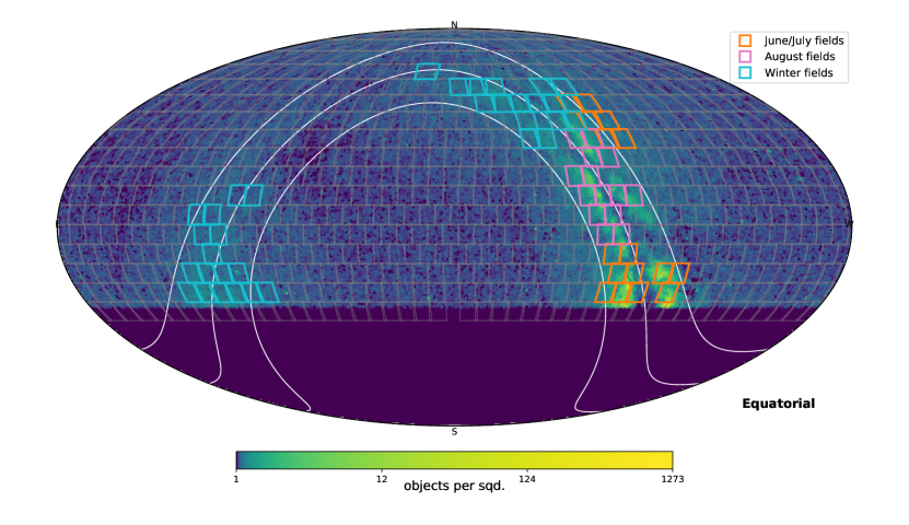
Figure 1: Sky density of candidate white dwarfs and hot subdwarfs selected from Gaia DR2 with the selected fields of the ZTF high-cadence Galactic Plane survey observed in ZTF year-1. The squares show individual ZTF fields which have been observed in high-cadence Galactic Plane observations. The white lines correspond to the Galactic equator and $|b|=15$ deg

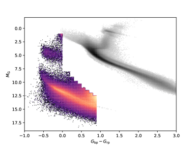
Figure 2: Hertzsprung Russell diagram of the objects used for the field selection. The grey shaded region corresponds to the underlying Hertzsprung Russell diagram showing the position of the main sequence and the red giant branch. The color-coded region corresponds to the objects which were selected for the field selection. The clump around $M_{\rm G}\approx 5$ corresponds to the hot subdwarfs whereas the region below corresponds to the white dwarfs.

As part of the Zwicky Transient Facility (ZTF), the Palomar 48-inch (P48) telescope images the sky every clear night conducting several surveys including a Northern Sky Survey with a 3-day cadence, as well as smaller surveys such as a 1-day Galactic Plane survey and simultaneous observations of the Northern TESS sectors (Graham et al., 2019; Bellm et al., 2019a, b; van Roestel et al., 2019). As part of the partnership share of ZTF we conducted a dedicated high-cadence Galactic Plane survey with a cadence of 40 sec at low Galactic latitudes aiming to find ultracompact binaries and compact pulsators. During that dedicated survey we either observed one field or alternated between two adjacent fields continuously for $\approx$1.5-3 hours on two to three consecutive nights in the ZTF-$r$ band. Here we present an overview of the ZTF high-cadence Galactic Plane survey executed in ZTF year 1. We present the observing strategy as well as some survey statistics. We show a progress report and finalize with some early results from the survey. In Section 2 we discuss the observing strategy as well as the field selection and the data processing. In Section 3 we present results for four representative fields and in Section 4 we give a progress report of already published results. In Section 5 we show some new early results from the high-cadence Galactic Plane survey and summarize and conclude in Section 6.

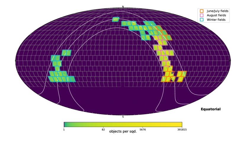
Figure 3: Sky density of individual objects with at least 80 epochs from the ZTF high-cadence Galactic Plane survey observed in ZTF year-1. The squares show individual ZTF fields which have been observed in high-cadence Galactic Plane observations. The white lines correspond to the Galactic equator and $|b|=15$ deg

2 Design of the high-cadence Galactic Plane survey

ZTF uses a 47 deg² camera consisting of 16 individual CCDs each 6k$\times$6k covering the full focal plane of the P48 telescope. The ZTF high-cadence Galactic Plane survey covered a total of $\approx$2990 deg² split in 64 individual ZTF fields observed over three observing blocks; mid-June to July 2018, two weeks in August 2018 and November 15th 2018 to January 15th 2019. All observations of the high-cadence Galactic Plane survey were obtained in ZTF-$r$ band. Each fields has $\approx 200-400$ epochs. The images were processed using ZTF data processing pipeline described in full detail in Masci et al. (2019).

During June and July we observed 16 fields covering $\approx 750$ deg² mostly at low Galactic longitudes. In June we observed every field continuously for 1hr15min and in July for 1hr25min. All fields were observed over $2$ or $3$ consecutive nights. In August, 14 fields covering $\approx 650$ deg² were observed over two weeks (see Tab. 1). We alternated between two adjacent fields continuously for 2hrs 40min each night. The same fields were repeated the following night. The observations in June/July and August were done under stable conditions with an average seeing of $\approx 2$ arcsec. We lost only a total of 5 nights due to weather during June/July and August observations.

Between 2018 November 15 and 2019 January 15 high-cadence Galactic Plane observations were scheduled for every night. We observed an additional 33 fields covering $\approx 1550$ deg² with stable weather conditions (see Tab. 1). The overall strategy varied during those two months due to unstable weather. Most fields were observed alternating with adjacent fields but in particular low declination fields were observed continuously. Because more time was available each night most fields were observed for $\approx$3 hrs. However, due to the unstable weather conditions about half of the fields were only observed in a single night and not repeated in subsequent nights. All other fields were observed over $2$ or $3$ nights. Although the seeing varies strongly between 1.7 arcsec and 4 arcsec, each field has a limiting magnitude of $>19.5$ mag. A detailed overview of the fields observed in stable weather conditions is given in the Appendix in Table 3, 4 and 5.

2.1 Field selection

The main science driver for the survey is to find and study UCBs consisting of fully degenerate or semi-degenerate stars. Hence we selected ZTF fields based on the density of objects residing well below the main-sequence, including mostly white dwarfs and hot subdwarf stars.

To achieve this, we extracted objects with absolute magnitudes which placed them below the main-sequence based on Gaia data release 2 (Gaia Collaboration et al., 2016, 2018). Only objects with declinations $>-30^{\circ}$ were selected. As the goal was not to extract a clean sample we used a very relaxed tolerance for the parallax precision ($\varpi/\sigma_{\varpi}>3$) and did not include any additional quality cuts, resulting in $\approx$350,000 individual objects (Fig. 2). For each object the ZTF field was calculated and the fields with the largest number of individual objects were selected for our survey. Selected fields with the highest density have $\approx 1000$ selected objects per deg². The final field selection was mainly driven by stellar density but also included other aspects like visibility and weather. Fig. 1 shows the sky density of the selected sources overplotted with the fields observed as part of the high-cadence Galactic Plane survey. As the stellar density is highest at low Galactic latitudes most fields are located at Galactic latitudes $\leq 15$ deg.

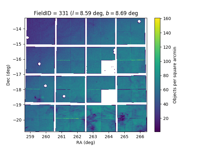
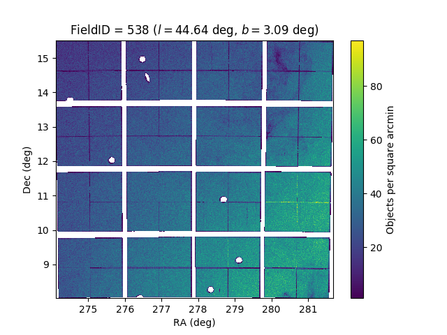
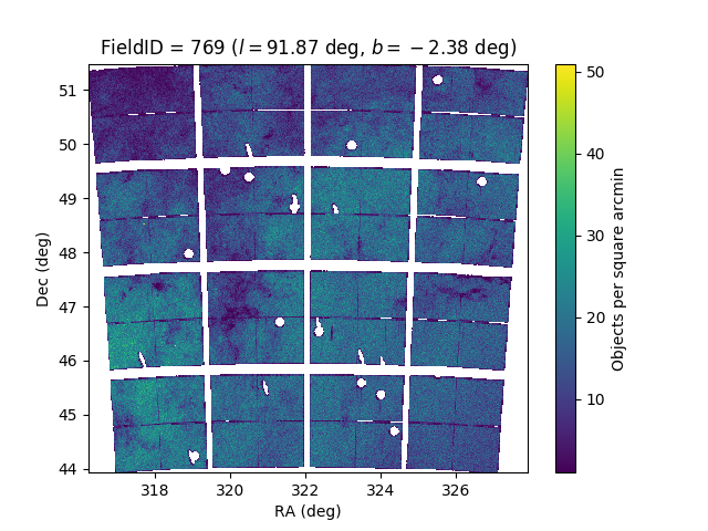
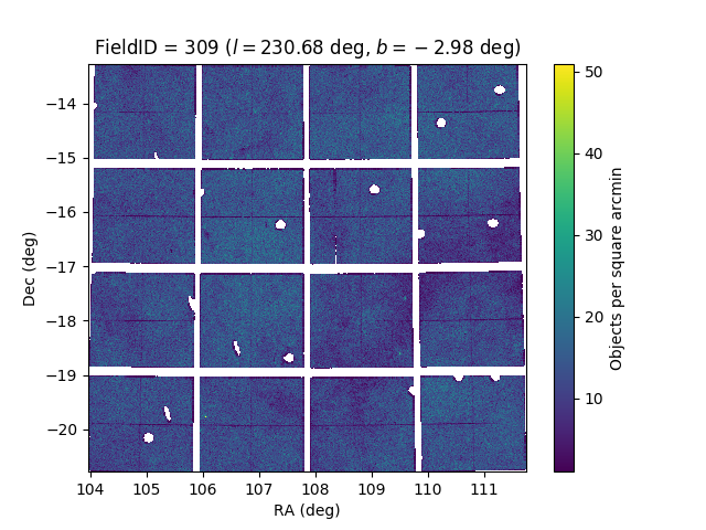
Figure 4: Sky density of ZTF objects with at least 80 epochs obtained during the high-cadence Galactic Plane survey for four selected fields. The white circles are masked regions due to saturated stars and the horizontal and vertical gaps are chip gaps between the 16 CCDs. The two white square areas in FieldID 331 are individual quadrants which were not processed.

2.2 Data processing and light curve extraction

Data processing and light curve generation follows the standard procedure for ZTF and occurs at the Infrared Processing and Analysis Center, Caltech. The raw camera image data is first instrumentally calibrated and astrometric solutions are derived using the Gaia DR1 catalog. Sources are detected and fluxes measured using both aperture (Bertin & Arnouts, 1996) and PSF-fit photometry (Stetson, 1987). Sources are photometrically calibrated using the Pan-STARRS1 DR1 catalog. The epochal image data are then co-added within their respective survey fields and camera readout channels to construct reference images. Each reference image is constructed using a minimum of 15 and maximum of 40 good quality epochal images, yielding depths of $\approx 2-2.5$ mag deeper than the single-epoch images.

The reference image co-adds are archived for use in other downstream processing: image differencing and light curve construction. To support light curve generation, sources are first detected and extracted from each reference image using PSF-fit photometry by running the DAOPhot utility (Stetson, 1987). These sources provide the seeds to facilitate positional cross-matching across all the single-epoch-based PSF extraction catalogs going back to the beginning of the survey. PSF-fitting on the single epoch images is also performed using DAOPhot. These single epoch images are direct single exposure images, not difference images. A fixed source-match radius of 1.5 arcsec is used for the positional matching. Only the PSF-fit-derived positions and photometry, along with selected PSF-fit metrics are retained during the source-matching process. Aperture photometry is not propagated to the light curve metadata.

Further details of the data processing, PSF-fit photometry software, light curve generation, formats, and overall performance on photometric accuracy are described in Masci et al. (2019). We extracted the light curves from each object which has at least $80$ epochs obtained as part of the high-cadence Galactic Plane survey from the ZTF light curve database “Kowalski” and extracted a total of $\approx 230$ million light curves across all observed fields. Figure 3 shows the sky density of the extracted objects overplotted with the fields observed as part of the high-cadence Galactic Plane survey.

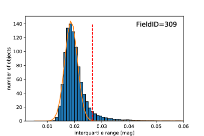
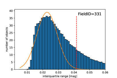
Figure 5: Histogram of the interquartile range extracted at a ZTF-$r$ median magnitude between 15.5 and 16 with the best Gaussian fit and the limit above which an object is called variable. The fit to the histogram in FieldID=331 is poor which is likely due to a large number of blended sources. See Sec. 3 for more details.

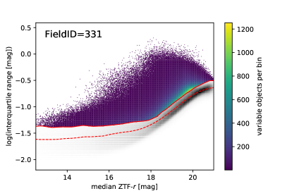
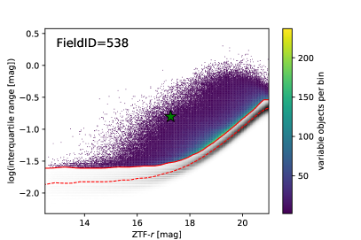
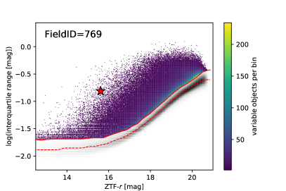
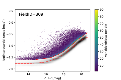
Figure 6: Interquartile range for each field. The grey shaded region corresponds to the underlying distribution of all objects in that field. The color-coded region corresponds to the objects which are possibly variable. The dashed red line shows the robust median of the underlying grey shaded region. The solid red line corresponds to the limit for potentially variable objects. The red star marks the position of ZTF J2130 (Kupfer et al., 2020a) and the green star marks the position of high-gravity BLAP-3 (Kupfer et al., 2019b).

3 Results from representative fields

We select four representative fields with different stellar densities and calculate statistics for each individual light curve, including median magnitude, reduced $\chi^{2}$, interquartile range, skewness, inverse von-Neumann, Stetson J and Stetson K statistics. We refer to Table 2 in Coughlin et al. (2020) for a detailed description of the individual statistics. These statistics are used to evaluate light curve variability and identify variable objects in the high-cadence Galactic Plane data.

The selected fields are FieldID=331 ($l=8.59$ deg, $b=8.69$ deg), FieldID=538 ($l=44.64$ deg, $b=3.09$ deg), FieldID=769 ($l=91.87$ deg, $b=-2.38$ deg) and FieldID=309 ($l=230.68$ deg, $b=-2.98$ deg). Figure 4 shows the stellar density of the four selected fields. The different coloring correspond to different densities. Some structure of lower and higher density regions can be seen in the fields. The white circles are masked regions due to saturated stars and the horizontal and vertical gaps are chip gaps between the 16 CCDs. The two white square areas in FieldID 331 are individual quadrants which were not processed. FieldID=331 was observed in three consecutive nights for 1.5 hrs each night. FieldID=538 was observed for two consecutive nights for 1.5 hrs and 2.5 hrs. FieldID=769 was observed for two consecutive nights for 3 hrs per night and FieldID=309 was observed for two consecutive nights for 1.7 hrs and 3 hrs. See Table 3, 4 and 5 for more details. The four selected fields represent a large range of stellar densities from $\approx 10$ million individual light curves for FieldID=331, $\approx 5.8$ million for FieldID=538, $\approx 3.8$ million for FieldID=769 and $\approx 2.3$ million for FieldID=309.

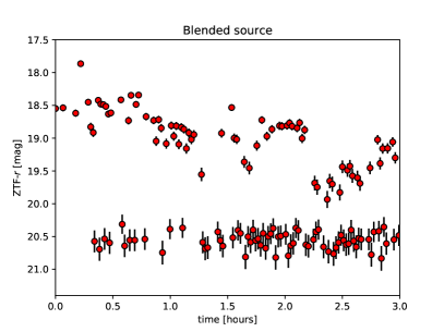
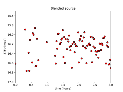
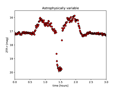
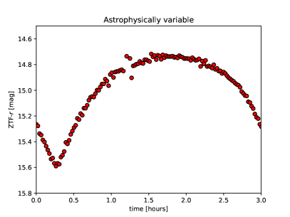
Figure 7: Example light curves of blended sources (upper panels) and real astrophysical variable sources (lower panels).

Different statistics can be used to evaluate whether an object is considered variable or not. We decided to use the interquartile range (IQR) which corresponds to the difference between the upper and lower quartile value. The main advantage of IQR is that it is a robust statistic not affected by extreme outliers due to individual bad photometry data points and therefore a better estimate of the general spread around the median magnitude. When there are outliers in a sample, the median and IQR are best used to summarize a typical value and the variability in the sample, respectively. Large variability in the light curve leads to a larger IQR.

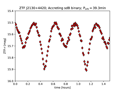
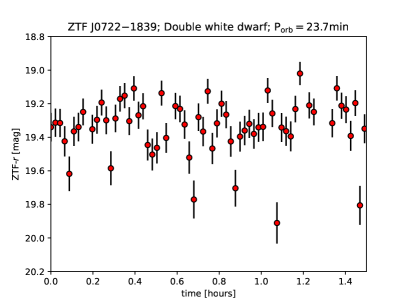
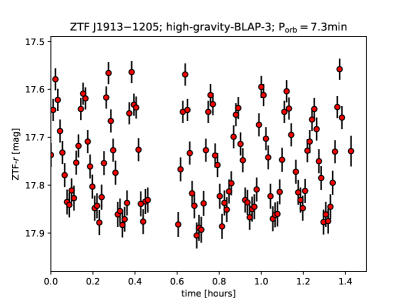
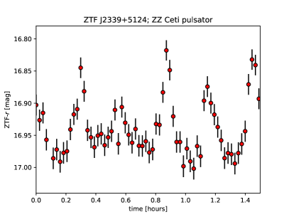
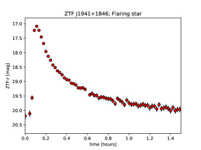
Figure 8: Example light curves of different types of variable objects discovered in the high-cadence Galactic Plane survey. Upper left panel: Accreting sdB binary (Kupfer et al., 2020a). Upper right panel: Eclipsing double white dwarf (Burdge et al., 2020a). Middle left panel: Compact radial mode pulsator (Kupfer et al., 2019b). Middle right panel: ZZ Ceti pulsator (Guidry et al., 2020). Lowest panel: Flaring star.

To estimate whether an object is variable in the high-cadence Galactic Plane data we used the following approach. We calculate the median ZTF-$r$ band magnitude for each object. The full magnitude range of all objects in a ZTF field is binned into several bins and each object is added to a bin based on its median magnitude. We used bin sizes of 0.5 mag between 12 and 16.5 mag where the IQR is constant at $\approx 0.02$ mag for non-variable sources. Above 16.5 mag we used bin sizes of 0.2 mag because the IQR for non-variable sources is increasing with increasing magnitudes to $\approx 0.2$ mag at the faint end at ZTF-$r$=20.5 mag because the underlying noise of the sources is increasing for fainter sources. Each bin contains at least a few thousand objects.

For each magnitude bin, we then calculate a histogram of IQR values. If there are only constant sources with a similar noise pattern, a normal distribution in an IQR histogram is expected. An excess of variable light curves will result in a deviation from a normal distribution towards more objects with larger IQR values. To estimate the excess and number of variable objects we fit a Gaussian to each IQR histogram and define an object as variable if, in a given histogram bin, less than $5\,\%$ of the sources in that magnitude bin are considered constant based on the Gaussian fit. Figure 5 shows two examples of IQR histograms with Gaussian fits of FieldID=309 and FieldID=331 for the magnitude range 15.5 - 16 mag. The orange curve corresponds to the Gaussian fit of the underlying histogram and the red dashed line corresponds to the IQR limit above which we call an object a variable.

Using this method we find $15\,\%$ variable sources for FieldID=331, $9\,\%$ variable sources for FieldID=769 and FieldID=538 and $5\,\%$ variable sources for FieldID=309 (see Fig. 6). The number of variable sources per field decreases with the stellar density of the field and it is likely that blending could produce false positives where the object appears variable due to a close-by source which contaminates the same pixel. To test that we inspected by eye 300 light curves which show the largest IQR for FieldID=331 which has the highest stellar density and FieldID=309 which has the lowest stellar densities of the selected fields. We find that astrophysically variable sources show a trend in the light curve, whereas non-astrophysically variable sources show typically rapid exposure-to-exposure variations. These variations can be explained in most cases by blending. Fig. 7 shows two examples of non-astrophysically variable sources and two examples of astrophysically variable sources. We find that out of the selected light curves only $15\,\%$ for FieldID=331 and $40\,\%$ for FieldID=309 show real astrophysical variability which shows that in the higher density fields the contamination of false positives is significantly larger. This is also consistent with the larger spread in IQR values seen in FieldID=331 compared to FieldID=309 (Fig. 5) because a larger number of false positives would lead to a larger spread of IQR values. Combining the variable sources with the fraction of real astrophysical variable sources we find that $\approx 1-2$ % of all sources show significant astrophysical variability in the high-cadence Galactic Plane data. We extracted $\approx 230$ million light curves and therefore expect a few million sources which show astrophysical photometric variability during the high-cadence Galactic Plane observations.

Table 2: Photometric properties of the high-gravity-BLAPs

Object	RA (J2000)	Dec (J2000)	$P$	$A_{\textrm{ZTF-r}}^{b}$	$\varpi^{c}$	$g^{a}$	$g-r^{a}$	FieldID
	(${}^{\textrm{h}}:^{\textrm{min}}:^{\textrm{sec}}$)	(${}^{\circ}:^{\prime}:^{\prime\prime}$)	(sec)	(mmag)	[mas]	(mag)	(mag)
ZTF-sdBV1	18:26:36.09	+10:00:22.3	$347.287\pm 0.02$	$19.9$	$0.5640\pm 0.0372$	14.90	$-$0.41	538
ZTF-sdBV2	19:13:54.77	$-$11:05:19.4	$360.576\pm 0.02$	$19.6$	$0.4568\pm 0.0888$	16.24	$-$0.33	385
ZTF-sdBV3	21:03:08.50	+44:43 14.9	$365.822\pm 0.01$	$53.3$	$0.3550\pm 0.0769$	16.07	$-$0.31	768
ZTF-sdBV4	08:06:07.05	$-$20:08 19.1	$370.481\pm 0.02$	$26.0$	$0.4021\pm 0.0531$	16.37	$-$0.32	311
ZTF-sdBV5	21:49:45.56	+45:58 36.5	$375.690\pm 0.02$	$36.1$	$0.3112\pm 0.0683$	16.55	$-$0.35	770
ZTF-sdBV6	07:40:00.71	$-$14:42 02.5	$375.782\pm 0.02$	$21.1$	$0.5979\pm 0.0394$	15.10	$-$0.36	310
ZTF-sdBV7	19:24:08.62	$-$12:58 30.9	$377.468\pm 0.02$	$19.3$	$0.7399\pm 0.0355$	14.64	$-$0.41	385
ZTF-sdBV8	06:54:48.55	$-$25:22 08.3	$435.459\pm 0.02$	$31.4$	$0.5458\pm 0.0318$	13.93	$-$0.44	259
ZTF-sdBV9	18:52:49.07	$-$18:46 08.4	$524.829\pm 0.02$	$73.4$	$0.1427\pm 0.1538$	17.12	$-$0.38	334
ZTF-sdBV10	19:49:59.34	+08:31 06.1	$646.306\pm 0.02$	$32.8$	$0.3884\pm 0.0642$	16.23	$-$0.38	541
ZTF-sdBV11	07:18:43.69	$-$02:29 31.2	$688.485\pm 0.02$	$30.2$	$0.1571\pm 0.1329$	17.52	$-$0.33	411
ZTF-sdBV12	17:07:41.34	$-$15:22 42.9	$995.479\pm 0.02$	$37.3$	$0.4376\pm 0.0346$	14.11	$-$0.35	330

^a from the Pan-STARRS release 1 (PS1) survey (Chambers et al., 2016) reddening corrected using Green et al. (2019)

^b amplitude in ZTF-$r$ from the ZTF light curves

^c parallaxes from Gaia EDR3 (Gaia Collaboration et al., 2016; Gaia Collaboration et al., 2020)

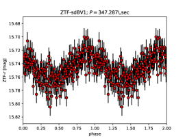
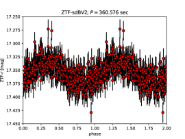
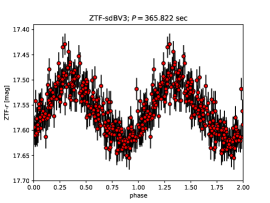
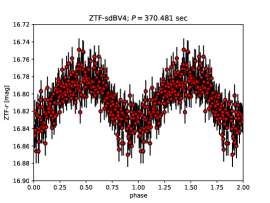
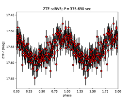
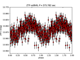
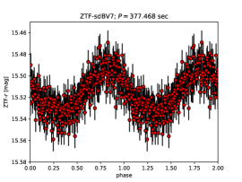
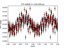
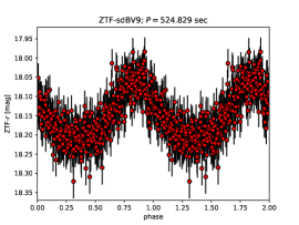
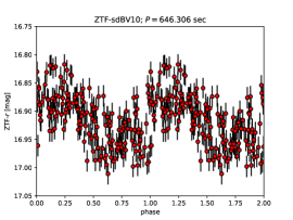
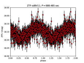
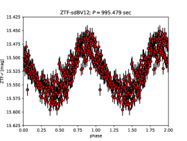
Figure 9: Phase folded ZTF light curves of the newly discovered radial mode sdB pulsators. All systems were discovered as part of the ZTF high-cadence Galactic Plane survey.

4 Progress report

The primary science driver for the survey is the detection and study of ultracompact binaries and rapid pulsators. Because the data volume is too large to inspect every single light curve we applied different cuts to pre-select light curves in early analysis. Depending on the science goal different selection criteria are required including a color cut using PanSTARRS DR2 colors or a selection based on the position in a color-magnitude diagram using Gaia DR2 (Gaia Collaboration et al., 2016, 2018). In a targeted search for hot subdwarf (sdB/sdO) binaries we cross-matched the catalogue of 40,000 hot subdwarf candidates (Geier et al., 2019) with the ZTF high-cadence Galactic plane data. These searches have already revealed some interesting discoveries, shown in Fig. 8.

As part of our cross-match with the hot subdwarf catalog we discovered ZTF J2130, the most compact sdB+WD binary and the first member of systems where the sdB fills its Roche Lobe and has started to transfer mass to the WD companion (Upper left panel Fig. 8; $P_{\rm orb}=39$ min; Kupfer et al. 2020a). In a follow-up search we discovered ZTF J2055, a second member of that class (Kupfer et al., 2020b). Both objects are only a few hundred million years old and members of the Galactic thin disc population, which explains why these objects have not been seen before and shows the value of a high-cadence Galactic Plane survey.

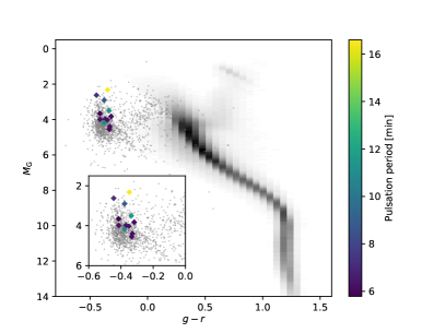
Figure 10: Hertzsprung Russell diagram of the newly discovered pulsators. The grey dots show known hot subdwarfs selected from Geier (2020) The grey shaded region corresponds to the underlying Hertzsprung Russell diagram showing the position of the main sequence and the red giant branch.

Burdge et al. (2020a) and Burdge et al. (2020b) presented 12 new ultracompact double white dwarfs including two new AM CVn systems, with orbital periods below one hour. Although the high-cadence Galactic Plane survey only covers $\approx$10 % of the ZTF sky almost half of the new ultracompact double white dwarfs have been covered by the high-cadence Galactic Plane observations including an 8.8 min binary (Burdge et al., 2020b). Due to the short eclipse duty cycle of $\leq$10 % for some systems, high-cadence Galactic Plane observations are ideal to cover enough in-eclipse points to recover the sources in period finding searches. The upper right panel in Fig. 8 displays an example of an eclipsing double white dwarf binary with an orbital period of 23.7 min (Burdge et al., 2020a). The lower points every 24 min indicate an eclipse and shows the short duty cycle of some of the eclipsing double white dwarfs.

The survey revealed a new class of large-amplitude radial-mode compact pulsators (three confirmed objects, middle left panel Fig. 8, Kupfer et al. 2019b). They show typical pulsation amplitudes of $5-20\,\%$ and periods between 3 min and 8 min. Although the stars reside in a region in the Hertzsprung Russell (HR) diagram usually occupied by helium core burning sdB stars, their pulsation properties are best explained with low-mass pre-He-WDs currently evolving through this part of the HR diagram contracting towards the He-WD cooling tracks. As such they could be the low mass version of the BLAPs.

The survey furthermore provided the necessary short-cadence observations to resolve the short-period pulsations of ZZ Cetis. These pulsations are evident in the middle right panel of Figure 8, which highlights ZTF J2339+5124, a new ZZ Ceti identified originally in Guidry et al. (2020). The typical diurnal mean sampling rate of ZTF is too short to resolve the pulsations for many pulsating white dwarfs (ZZ Ceti pulsation modes range from $100-1500$ sec Mukadam et al. 2013; Bognár et al. 2020). However, the Galactic Plane survey’s 40 sec sampling over the span of hours is sufficient to capture consecutive pulsation peaks in ZZ Cetis. These observations may then be coupled with an object’s placement relative to the pulsating white dwarf instability strip to allow for its confirmation as a ZZ Ceti (since pulsations are only driven in a narrow range of effective temperature, e.g., Gianninas et al. 2015), as done for ZTF 2339+5124.

The survey has also provided a large sample of stellar flare detections. These events are the result of rapid magnetic reconnection for low-mass stars, and typically have timescales of minutes to hours (Hawley et al., 2014), well-matched to the cadence of this survey. We can trace flare events in their entirety (e.g. lower panel Fig. 8), measuring precise flare energies when the distance is known, as opposed to flares being detected as single-point outliers in the primary ZTF survey. Using the first data release from the 14 August fields, more than 1500 stellar flare events have been detected (C. Klein et al., in prep). This large sample allows us to study correlations between flare occurrence rates and Galactic height.

5 Early results - new single-mode hot subdwarf pulsators

Subdwarf B stars (sdBs) are hot stars of spectral type B with luminosities below the main sequence. The formation mechanisms and evolution of sdBs is still debated, although most sdBs are thought to be helium (He)-burning stars with masses $\approx 0.5$ M${}_{\odot}\,$ and thin hydrogen envelopes (Heber 1986, 2009, 2016). Amongst the sdB stars, two types of multi-periodic pulsators have been discovered, both with generally milli-mag amplitudes. On the hotter side (T_eff$\gtrsim 28,000$ K) are the V361 Hya stars which are pressure mode ($p$-mode) pulsators with typical periods of a few minutes (Kilkenny et al., 1997). On the cooler side (T_eff$\lesssim 28,000$ K) are the V1093 Her stars which are gravity mode ($g$-mode) pulsators with periods of 45 min to 2 hours (Green et al., 2003). Only very few sdBs are know to show amplitudes up to a few percent (Østensen et al., 2010). This includes Balloon 090100001 and PG 1605+072, which are multi-periodic pulsators with photometric amplitudes of up to 60 mmag (Oreiro et al., 2004; Tillich et al., 2007).

Even before their discovery, the variability of sdBs was predicted to be caused by non-radial pulsation modes driven by the opacity bump due to partial ionization of iron (Charpinet et al., 1996, 1997; Fontaine et al., 2003). Until recently the only known single-mode sdB pulsator was CS 1246, with an amplitude of $\approx 30$ mmag which has decreased below its detection limit over the last few years (Barlow et al., 2010). Barlow et al. (2010) confirmed the object as radial-mode pulsator and found $R=0.19\pm 0.08$ R${}_{\odot}\,$  and $M=0.39^{+0.30}_{-0.13}$ M${}_{\odot}\,$using the Baade-Wesselink method. Pietrukowicz et al. (2017) discovered a new class of radial mode pulsators with large amplitudes up to $300-400$ mmag: the Blue-Large Amplitude pulsators (BLAPs). More recently a new class of radial mode hot subdwarf B type pulsators (high-gravity BLAPs) was discovered which show radial mode pulsation amplitudes up $150$ mmag (Kupfer et al., 2019b). Unlike most of the multi-periodic sdB pulsators, the BLAP and high-gravity BLAPS are more likely to be contracting low-mass helium pre-white dwarfs rather than compact He-core burning stars (Romero et al., 2018; Byrne & Jeffery, 2018, 2020).

We discovered 12 new sdB pulsators which show only a single pulsation mode as part of this survey. We find amplitudes in the ZTF-$r$ band between $20$ and $73$ mmag which are similar to CS 1246 (Barlow et al., 2010) but smaller than seen in the high-gravity BLAPs (Kupfer et al., 2019b). Each system exhibits only a single frequency in the light curve (see Fig. 9 for the phase folded light curves). The pulsation periods range from 5.8 minutes to 16 minutes. We performed a color correction for all objects using 3D extinction maps provided by Green et al. (2019) and find very similar PanSTARRS colors between $g-r=-0.3$ mag and $g-r=-0.45$ mag. Using the reddening corrected $g$-band magnitudes and parallaxes from Gaia EDR3 (Gaia Collaboration et al., 2016; Gaia Collaboration et al., 2020) we find absolute magnitudes in the range $\approx 2.5-4.5$ mag. Fig. 10 shows their position in a color-magnitude diagram color-coded with the pulsation period, which confirms that they are clustered in the region where hot subdwarf B stars are located. Table 2 presents an overview of the new pulsators. Remarkably, seven objects of our new sample show very similar pulsation periods around six minutes which is close to the pulsation period of CS 1246, indicating that some of these new pulsators might be related to CS 1246. If they are confirmed as radial-mode pulsators, like CS 1246, future follow-up observations will measure their masses and radii. Phase resolved spectroscopy and multi-band photometry to fully characterize the objects is underway.

6 Summary and Conclusions

We have presented an overview and first results of our dedicated high-cadence Galactic Plane survey for short period variable objects, carried out as part of ZTF during its first year of operation. We covered a total of 2990 deg² between June 2018 and January 2019 in ZTF-$r$. Each field was observed continuously at a cadence of 40 sec typically between $1.5$ and $3$ hours with some fields up $5-6$ hours. We only selected fields with at least $80$ epochs and most fields have between $200$ and $400$.

The survey covered a total of $\approx$230 million stars to a limiting magnitude of 20.5 mag in ZTF-$r$. Stellar densities range from 4 objects per arcmin² to $\approx$70 objects per arcmin². Four fields were selected for a detailed analysis. We calculate light curve statistics for each field and use the IQR to estimate the number of variable objects for each field. We find that $\approx 1-2\,\%$ of objects show astrophysical variability in each field which leads to $\approx 2-4$ million expected variable objects in the ZTF Galactic Plane high-cadence Galactic Plane data. The largest contaminant are blended sources. For the highest density field this contamination rate is high, with up to $90\,\%$ of the sources found to be variable from the IQR. This shows that simple light curve statistics can reduce the number of non-variable sources substantially but is not sufficient to select a clean sample in high-density fields. Additional measures are required. In future, instead of using direct (non-difference) images, we will explore the use of forced photometry on difference images using input seed positions provided by external catalogs, e.g., Gaia EDR3. This will provide a more complete census of photometric variability in confused regions of the Galactic Plane. Forced photometry is expected to decrease the number of wrong magnitudes due to blending. Additionally, van van Roestel et al. (2021) has shown that machine learning classification can also substantially decrease the number of false positives.

We have started to explore the data and present a progress report of recently published objects which were discovered by period searches using color-selected sub-samples. Some of these discoveries revealed new types of variable stars. In this work we also present a sample of 12 new single-mode hot subdwarf B-star pulsators with pulsation amplitudes between ZTF-$r=20-76$ mmag and pulsation periods between $P=5.8-16$ min. If they are confirmed as radial mode puslators future follow-up observations will measure their masses and radii.

Future work is in progress which applies machine learning techniques to classify large samples of individual objects (Coughlin et al., 2020; van Roestel et al., 2021). ZTF data up to December 2018 was released in data release 3 and the remaining data obtained in January 2019 was released in data release 4. ZTF has continued with high-cadence Galactic Plane observations in year 2 and 3. We settled on 140 epochs (1.5hrs) per field and continued to use ZTF-$r$ band. We aim to observe the entire Galactic Plane within $|b|<10$ and further out to high stellar density regions. We continue to analyse the data using period-finding algorithms and light curve statistics, but are also exploring the use of neural networks to identify and classify variable stars.

Looking ahead, the Vera Rubin Observatory’s Legacy Survey of Space and Time (LSST) will observe to fainter magnitudes and with an expected precision of $\sim$ 5 mmag is expected to find more variable sources (Huber et al., 2006). Given the significantly larger number of sources in the LSST the Galactic Plane observations of LSST are expected to observe unique sources which are too faint for ZTF but the high stellar density will challenge data analysis and the significantly higher number of sources will require more computational power to search all the objects.

Data Availability

All the observational data used in this paper are publicly available at the IRSA database and can be accessed here: https://www.ztf.caltech.edu/page/dr4.

Appendix A Fields observed as part of the high-cadence Galactic Plane observations in ZTF year-1

Table 3: Fields observed as part of the June/July campaign. Median values are given for limiting magnitude and seeing

Date	ZTF	RA	Dec	Gal Lat	Gal Long	epochs	limit	seeing	duration	fraction
UTC	FieldID	(deg)	(deg)	(deg)	(deg)		(mag)	(arcsec)	(hrs)	successful
06-16-18	284	279.8366	$-$24.2500	$-$8.9125	10.2331	23	20.72	1.98	0.23	0.98
06-17-18	284	279.8366	$-$24.2500	$-$8.9125	10.2331	113	20.58	2.26	1.23	0.96
06-18-18	284	279.8366	$-$24.2500	$-$8.9125	10.2331	107	20.39	2.51	1.16	0.99
06-20-18	330	255.5263	$-$17.0500	14.2859	4.7848	115	20.32	2.51	1.25	1.00
06-21-18	330	255.5263	$-$17.0500	14.2859	4.7848	115	20.36	2.21	1.25	1.00
06-22-18	385	287.6598	$-$9.8500	$-$9.2762	26.6514	115	20.54	2.34	1.38	0.73
06-23-18	385	287.6598	$-$9.8500	$-$9.2762	26.6514	115	20.47	2.15	1.25	0.81
06-24-18	385	287.6598	$-$9.8500	$-$9.2762	26.6514	115	20.07	2.42	1.25	0.88
06-25-18	766	292.6968	47.7500	13.4390	80.1691	113	20.75	1.59	1.27	1.00
06-26-18	766	292.6968	47.7500	13.4390	80.1691	113	20.47	1.82	1.27	1.00
06-27-18	766	292.6968	47.7500	13.4390	80.1691	111	20.32	1.90	1.28	1.00
06-28-18	727	287.0350	40.5500	14.0583	71.6873	115	20.05	2.33	1.25	1.00
06-29-18	727	287.0350	40.5500	14.0583	71.6873	137	19.74	3.35	1.49	1.00
06-30-18	684	282.5628	33.3500	14.4152	63.4051	133	20.34	2.13	1.45	1.00
07-01-18	684	282.5628	33.3500	14.4152	63.4051	133	20.33	1.84	1.45	1.00
07-03-18	280	257.8188	$-$24.2500	8.3828	0.0438	133	20.32	2.79	1.45	0.74
07-04-18	280	257.8188	$-$24.2500	8.3828	0.0438	132	20.37	2.22	1.44	0.67
07-05-18	331	262.5569	$-$17.0500	8.6904	8.5864	134	20.41	2.33	1.46	0.49
07-06-18	331	262.5569	$-$17.0500	8.6904	8.5864	133	20.04	2.85	1.45	0.68
07-07-18	331	262.5569	$-$17.0500	8.6904	8.5864	133	20.33	2.44	1.45	0.72
07-08-18	282	272.4435	$-$24.2500	$-$2.9315	7.1078	133	20.26	2.31	1.45	0.43
07-09-18	282	272.4435	$-$24.2500	$-$2.9315	7.1078	135	20.09	2.52	1.47	0.44
07-11-18	283	279.8366	$-$24.2500	$-$8.9125	10.2331	116	20.14	2.40	1.26	0.40
07-12-18	283	279.8366	$-$24.2500	$-$8.9125	10.2331	132	20.26	2.25	1.44	0.47
07-13-18	283	279.8366	$-$24.2500	$-$8.9125	10.2331	133	20.27	2.30	1.45	0.46
07-14-18	333	276.6440	$-$17.0500	$-$2.9817	15.3198	133	20.01	2.22	1.45	0.23
07-15-18	333	276.6440	$-$17.0500	$-$2.9817	15.3198	133	19.97	2.34	1.45	0.32
07-16-18	333	276.6440	$-$17.0500	$-$2.9817	15.3198	136	19.86	2.17	1.48	0.54
07-17-18	384	280.6106	$-$9.8500	$-$3.0783	23.4976	134	20.22	2.23	1.48	0.40
07-18-18	384	280.6106	$-$9.8500	$-$3.0783	23.4976	125	20.52	2.09	1.36	0.36
07-19-18	384	280.6106	$-$9.8500	$-$3.0783	23.4976	136	20.26	2.16	1.48	0.33
07-20-18	334	283.7259	$-$17.0500	$-$9.0209	18.3982	135	20.01	2.63	1.47	0.72
07-21-18	334	283.7259	$-$17.0500	$-$9.0209	18.3982	136	20.14	1.97	1.48	1.00
07-22-18	334	283.7259	$-$17.0500	$-$9.0209	18.3982	136	20.10	2.02	1.48	1.00
07-23-18	683	274.7095	33.3500	20.5066	60.8553	137	20.63	1.73	1.49	1.00
07-24-18	683	274.7095	33.3500	20.5066	60.8553	134	20.39	1.80	1.46	1.00
07-25-18	726	278.4181	40.5500	20.1368	69.1476	133	20.10	1.86	1.45	1.00
07-26-18	726	278.4181	40.5500	20.1368	69.1476	133	20.03	1.85	1.45	1.00
07-27-18	765	282.9221	47.7500	19.4902	77.5052	133	20.20	1.72	1.45	1.00
07-28-18	765	282.9221	47.7500	19.4902	77.5052	133	20.06	1.70	1.45	1.00
07-29-18	330	255.5263	$-$17.0500	14.2859	4.7848	69	19.91	1.75	1.19	1.00
07-31-18	282	272.4435	$-$24.2500	$-$2.9315	7.1078	100	19.71	2.12	1.08	0.80

Table 4: Fields observed as part of the August campaign. Median values are given for limiting magnitude and seeing

Date	ZTF	RA	Dec	Gal Lat	Gal Long	epochs	limit	seeing	duration	fraction
UTC	FieldID	(deg)	(deg)	(deg)	(deg)		(mag)	(arcsec)	(hrs)	successful
08-03-2018	538	284.8764	11.7500	3.0889	44.6385	118	20.84	1.87	1.28	1.00
08-03-2018	539	277.9013	11.7500	9.1851	41.5422	42	20.66	1.97	0.45	1.00
08-04-2018	538	284.8764	11.7500	3.0889	44.6385	118	20.93	1.87	2.59	1.00
08-04-2018	539	277.9013	11.7500	9.1851	41.5422	118	20.76	2.19	2.59	1.00
08-07-2018	638	285.7714	26.1500	2.9069	61.0817	118	21.09	1.89	2.67	1.00
08-07-2018	639	293.2531	26.1500	$-$2.8742	64.5379	118	20.97	2.08	2.67	1.00
08-08-2018	638	285.7714	26.1500	2.9069	61.0817	118	21.03	1.84	2.67	1.00
08-08-2018	639	293.2531	26.1500	$-$2.8742	64.5379	118	20.90	2.03	2.67	1.00
08-10-2018	488	288.1194	4.5500	$-$3.0953	39.7486	118	20.55	2.01	2.59	1.00
08-10-2018	489	295.1303	4.5500	$-$9.2520	43.0768	118	20.42	2.14	2.59	1.00
08-11-2018	540	291.9311	11.7500	$-$3.0068	47.8872	54	20.52	2.00	2.31	1.00
08-11-2018	541	298.9153	11.7500	$-$8.9492	51.2901	55	20.54	2.04	1.26	1.00
08-12-2018	540	291.9311	11.7500	$-$3.0068	47.8872	117	20.67	2.12	2.57	1.00
08-12-2018	541	298.9153	11.7500	$-$8.9492	51.2901	116	20.57	2.22	2.55	1.00
08-13-2018	591	296.1269	18.9500	$-$2.9775	56.1558	118	20.80	2.09	2.61	1.00
08-13-2018	592	303.3767	18.9500	$-$8.8128	59.7765	118	20.85	2.01	2.61	1.00
08-14-2018	591	296.1269	18.9500	$-$2.9775	56.1558	118	20.92	1.87	2.63	1.00
08-14-2018	592	303.3767	18.9500	$-$8.8128	59.7765	118	20.95	1.95	2.63	1.00
08-15-2018	685	290.4160	33.3500	8.4910	66.2776	117	20.92	1.95	2.77	1.00
08-15-2018	686	298.2693	33.3500	2.7706	69.5025	117	20.77	2.09	2.77	1.00
08-16-2018	685	290.4160	33.3500	8.4910	66.2776	112	20.93	1.81	2.81	0.85
08-16-2018	686	298.2693	33.3500	2.7706	69.5025	111	20.81	1.95	2.79	0.86
08-17-2018	436	284.3894	$-$2.65000	$-$3.1176	31.6292	97	20.37	2.19	2.79	0.98
08-17-2018	437	291.4182	$-$2.65000	$-$9.3570	34.8701	94	20.47	2.12	2.79	1.00
08-18-2018	436	284.3894	$-$2.65000	$-$3.1176	31.6292	118	20.51	2.16	2.57	0.97
08-18-2018	437	291.4182	$-$2.65000	$-$9.3570	34.8701	118	20.61	2.04	2.57	1.00

Table 5: Fields observed as part of the winter campaign. Median values are given for limiting magnitude and seeing

Date	ZTF	RA	Dec	Gal Lat	Gal Long	epochs	limit	seeing	duration	fraction
UTC	FieldID	(deg)	(deg)	(deg)	(deg)		(mag)	(arcsec)	(hrs)	successful
11-15-2018	728	295.6518	40.5500	8.2113	74.6857	148	19.93	2.81	3.29	1.00
11-15-2018	729	304.2686	40.5500	2.6520	78.1565	148	20.04	2.74	3.29	1.00
11-19-2018	799	291.0910	54.9500	17.3604	86.5193	145	20.16	1.72	3.32	0.92
11-19-2018	800	302.1884	54.9500	11.7051	89.5415	146	20.08	1.74	3.90	0.90
11-26-2018	767	302.4714	47.7500	7.7191	83.4543	128	20.30	1.81	2.88	1.00
11-26-2018	768	312.2461	47.7500	2.4194	87.3502	128	20.42	1.81	2.88	1.00
11-27-2018	688	313.8717	33.3500	$-$7.8072	77.1136	156	20.41	2.14	4.10	0.99
11-27-2018	689	321.6554	33.3500	$-$12.5790	81.6002	158	20.48	2.20	4.20	1.00
11-28-2018	688	313.8717	33.3500	$-$7.8072	77.1136	142	19.66	1.91	3.75	0.80
11-28-2018	689	321.6554	33.3500	$-$12.5790	81.6002	142	19.78	1.87	3.76	0.86
11-29-2018	767	302.4714	47.7500	7.7191	83.4543	127	20.62	1.81	2.86	1.00
11-29-2018	768	312.2461	47.7500	2.4194	87.3502	133	20.67	1.80	2.86	1.00
12-03-2018	730	312.8218	40.5500	$-$2.5179	82.0919	59	20.62	1.81	1.30	1.00
12-03-2018	731	321.3116	40.5500	$-$7.2339	86.5070	109	20.67	1.80	1.84	0.98
12-03-2018	259	104.6634	$-$24.2500	$-$8.9125	235.7669	180	20.67	1.80	1.96	0.95
12-04-2018	411	107.1700	$-$2.6500	3.1405	217.6228	275	20.29	2.25	6.02	0.85
12-04-2018	412	114.2600	$-$2.6500	9.3964	220.9648	276	20.30	2.30	6.02	0.86
12-05-2018	411	107.1700	$-$2.6500	3.1405	217.6228	275	20.36	2.41	6.04	1.00
12-05-2018	412	114.2600	$-$2.6500	9.3964	220.9648	275	20.39	2.46	6.01	1.00
12-09-2018	770	332.1016	47.7500	$-$6.6404	97.1225	134	20.24	2.35	3.97	1.00
12-09-2018	771	342.1387	47.7500	$-$10.1214	102.9618	132	20.42	2.26	3.95	1.00
12-09-2018	259	104.6634	$-$24.2500	$-$8.9125	235.7669	111	19.77	2.19	1.26	0.95
12-12-2018	308	100.7741	$-$17.0500	$-$9.0209	227.6018	140	20.32	2.53	3.05	0.97
12-12-2018	309	107.8560	$-$17.0500	$-$2.9817	230.6802	140	20.26	2.66	3.05	1.00
12-13-2018	308	100.7741	$-$17.0500	$-$9.0209	227.6018	78	19.96	3.16	1.69	1.00
12-13-2018	309	107.8560	$-$17.0500	$-$2.9817	230.6802	78	19.99	3.14	1.69	1.00
12-13-2018	769	322.0645	47.7500	$-$2.3827	91.8751	269	19.83	3.35	2.94	1.00
12-14-2018	769	322.0645	47.7500	$-$2.3827	91.8751	270	20.06	2.36	2.95	0.92
12-16-2018	803	335.1841	54.9500	$-$1.7248	102.7388	345	20.21	2.11	3.77	1.00
12-16-2018	257	89.8772	$-$24.2500	$-$21.2513	230.1444	198	20.42	2.02	2.16	1.00
12-17-2018	512	92.5688	11.7500	$-$3.0068	198.1128	201	19.85	1.93	6.14	0.87
12-17-2018	513	99.6235	11.7500	3.0889.	201.3615	201	19.90	1.94	6.14	0.87
12-19-2018	257	89.8772	$-$24.2500	$-$21.2513	230.1444	189	19.74	2.50	2.06	1.00
12-20-2018	257	89.8772	$-$24.2500	$-$21.2513	230.1444	188	19.60	2.42	2.05	1.00
12-22-2018	807	20.0000	62.1500	$-$0.2329	126.6119	271	19.91	1.82	2.96	1.00
12-22-2018	310	114.9123	$-$17.0500	2.9306	233.9298	279	19.30	2.36	3.05	0.91
12-23-2018	807	20.0000	62.1500	$-$0.2329	126.6119	270	19.82	2.11	2.95	1.00
12-23-2018	310	114.9123	$-$17.0500	2.9306	233.9298	136	19.41	2.18	1.48	0.94
12-24-2018	804	345.7743	54.9500	$-$4.5684	108.1171	153	20.06	1.75	3.49	0.94
12-24-2018	805	356.3646	54.9500	$-$6.5258	113.8966	153	20.17	1.71	3.49	0.95
12-24-2018	260	112.0564	$-$24.2500	$-$2.9315	238.8922	189	19.52	2.10	2.06	0.81
12-28-2018	804	345.7743	54.9500	$-$4.5684	108.1171	58	19.60	3.87	1.31	0.82
12-28-2018	805	356.3646	54.9500	$-$6.5258	113.8966	87	19.83	3.57	1.28	0.88
12-28-2018	260	112.0564	$-$24.2500	$-$2.9315	238.8922	196	19.44	3.83	2.14	0.94
12-29-2018	806	6.6666	62.1500	$-$0.3373	120.3949	87	19.86	3.84	0.84	1.00
12-29-2018	260	112.0564	$-$24.2500	$-$2.9315	238.8922	196	19.75	3.25	2.14	1.00
12-30-2018	462	110.1486	4.5500	9.0982	212.5713	275	20.09	2.91	6.01	0.98
12-30-2018	463	116.9904	4.5500	15.1705	215.7493	274	20.09	2.96	5.99	0.98

Table A3 continued.
Date	ZTF	RA	Dec	Gal Lat	Gal Long	epochs	limit	seeing	duration	fraction
UTC	FieldID	(deg)	(deg)	(deg)	(deg)		(mag)	(arcsec)	(hrs)	successful
01-03-2019	261	119.3957	$-$24.2500	2.8444	242.2711	172	19.55	4.05	1.87	0.93
01-04-2019	261	119.3957	$-$24.2500	2.8444	242.2711	171	20.00	2.83	1.83	1.00
01-04-2019	258	97.2703	$-$24.2500	$-$15.0272	232.8673	163	20.22	2.60	1.78	1.00
01-08-2019	360	110.9488	$-$9.8500	3.0707	225.7543	333	19.91	3.57	3.64	0.91
01-10-2019	262	126.6811	$-$24.2500	8.3828	245.9562	172	20.32	2.29	1.87	0.95
01-10-2019	260	112.0564	$-$24.2500	$-$2.9315	238.8922	159	20.13	2.58	1.73	1.00
01-11-2019	311	121.9430	$-$17.0500	8.6904	237.4136	275	20.58	2.32	3.00	1.00

References

- Baker et al. (2019) Baker J., et al., 2019, BAAS, 51, 123
- Barclay et al. (2011) Barclay T., Ramsay G., Hakala P., Napiwotzki R., Nelemans G., Potter S., Todd I., 2011, MNRAS, 413, 2696
- Barlow et al. (2010) Barlow B. N., et al., 2010, MNRAS, 403, 324
- Bellm et al. (2019a) Bellm E. C., et al., 2019a, PASP, 131, 018002
- Bellm et al. (2019b) Bellm E. C., et al., 2019b, PASP, 131, 068003
- Bertin & Arnouts (1996) Bertin E., Arnouts S., 1996, A&AS, 117, 393
- Bognár et al. (2020) Bognár Z., et al., 2020, A&A, 638, A82
- Breger (2000) Breger M., 2000, in Breger M., Montgomery M., eds, Astronomical Society of the Pacific Conference Series Vol. 210, Delta Scuti and Related Stars. p. 3
- Burdge et al. (2019) Burdge K. B., et al., 2019, Nature, 571, 528
- Burdge et al. (2020a) Burdge K. B., et al., 2020a, ApJ, 905, 32
- Burdge et al. (2020b) Burdge K. B., et al., 2020b, ApJ, 905, L7
- Byrne & Jeffery (2018) Byrne C. M., Jeffery C. S., 2018, MNRAS, 481, 3810
- Byrne & Jeffery (2020) Byrne C. M., Jeffery C. S., 2020, MNRAS, 492, 232
- Chambers et al. (2016) Chambers K. C., et al., 2016, arXiv e-prints,
- Charpinet et al. (1996) Charpinet S., Fontaine G., Brassard P., Dorman B., 1996, ApJ, 471, L103
- Charpinet et al. (1997) Charpinet S., Fontaine G., Brassard P., Chayer P., Rogers F. J., Iglesias C. A., Dorman B., 1997, ApJ, 483, L123
- Coughlin et al. (2020) Coughlin M. W., et al., 2020, arXiv e-prints, p. arXiv:2009.14071
- Fontaine & Brassard (2008) Fontaine G., Brassard P., 2008, PASP, 120, 1043
- Fontaine et al. (2003) Fontaine G., Brassard P., Charpinet S., Green E. M., Chayer P., Billères M., Randall S. K., 2003, ApJ, 597, 518
- Gaia Collaboration et al. (2016) Gaia Collaboration et al., 2016, A&A, 595, A1
- Gaia Collaboration et al. (2018) Gaia Collaboration et al., 2018, A&A, 616, A1
- Gaia Collaboration et al. (2020) Gaia Collaboration Brown A. G. A., Vallenari A., Prusti T., de Bruijne J. H. J., Babusiaux C., Biermann M., 2020, arXiv e-prints, p. arXiv:2012.01533
- Geier (2020) Geier S., 2020, A&A, 635, A193
- Geier et al. (2019) Geier S., Raddi R., Gentile Fusillo N. P., Marsh T. R., 2019, A&A, 621, A38
- Gianninas et al. (2015) Gianninas A., Kilic M., Brown W. R., Canton P., Kenyon S. J., 2015, ApJ, 812, 167
- Graham et al. (2019) Graham M. J., et al., 2019, arXiv e-prints,
- Green et al. (2003) Green E. M., et al., 2003, Ap&SS, 284, 65
- Green et al. (2019) Green G. M., Schlafly E., Zucker C., Speagle J. S., Finkbeiner D., 2019, ApJ, 887, 93
- Guidry et al. (2020) Guidry J. A., et al., 2020, arXiv e-prints, p. arXiv:2012.00035
- Hawley et al. (2014) Hawley S. L., Davenport J. R. A., Kowalski A. F., Wisniewski J. P., Hebb L., Deitrick R., Hilton E. J., 2014, ApJ, 797, 121
- Heber (1986) Heber U., 1986, A&A, 155, 33
- Heber (2009) Heber U., 2009, ARA&A, 47, 211
- Heber (2016) Heber U., 2016, PASP, 128, 082001
- Heinze et al. (2018) Heinze A. N., et al., 2018, AJ, 156, 241
- Hermes et al. (2013) Hermes J. J., et al., 2013, ApJ, 765, 102
- Huber et al. (2006) Huber M. E., Everett M. E., Howell S. B., 2006, The Astronomical Journal, 132, 633–649
- Jayasinghe et al. (2018) Jayasinghe T., et al., 2018, MNRAS, 477, 3145
- Kilkenny et al. (1997) Kilkenny D., Koen C., O’Donoghue D., Stobie R. S., 1997, MNRAS, 285, 640
- Korol et al. (2017) Korol V., Rossi E. M., Groot P. J., Nelemans G., Toonen S., Brown A. G. A., 2017, MNRAS, 470, 1894
- Kremer et al. (2017) Kremer K., Breivik K., Larson S. L., Kalogera V., 2017, ApJ, 846, 95
- Kupfer et al. (2017) Kupfer T., et al., 2017, ApJ, 851, 28
- Kupfer et al. (2018) Kupfer T., et al., 2018, MNRAS, 480, 302
- Kupfer et al. (2019a) Kupfer T., Kilic M., Maccarone T., Burns E., Fryer C. L., Wilson-Hodge C. A., 2019a, BAAS, 51, 188
- Kupfer et al. (2019b) Kupfer T., et al., 2019b, ApJ, 878, L35
- Kupfer et al. (2020a) Kupfer T., et al., 2020a, ApJ, 891, 45
- Kupfer et al. (2020b) Kupfer T., et al., 2020b, ApJ, 898, L25
- Lamberts et al. (2019) Lamberts A., Blunt S., Littenberg T. B., Garrison-Kimmel S., Kupfer T., Sanderson R. E., 2019, MNRAS, 490, 5888
- Law et al. (2009) Law N. M., et al., 2009, PASP, 121, 1395
- Littenberg et al. (2013) Littenberg T. B., Larson S. L., Nelemans G., Cornish N. J., 2013, MNRAS, 429, 2361
- Littenberg et al. (2019) Littenberg T., et al., 2019, BAAS, 51, 34
- Macfarlane et al. (2015) Macfarlane S. A., Toma R., Ramsay G., Groot P. J., Woudt P. A., Drew J. E., Barentsen G., Eislöffel J., 2015, MNRAS, 454, 507
- Macfarlane et al. (2017a) Macfarlane S. A., et al., 2017a, MNRAS, 465, 434
- Macfarlane et al. (2017b) Macfarlane S. A., et al., 2017b, MNRAS, 470, 732
- Masci et al. (2019) Masci F. J., et al., 2019, PASP, 131, 018003
- Meng et al. (2020) Meng X.-C., Han Z.-W., Podsiadlowski P., Li J., 2020, ApJ, 903, 100
- Mukadam et al. (2013) Mukadam A. S., et al., 2013, ApJ, 771, 17
- Nelemans et al. (2004) Nelemans G., Yungelson L. R., Portegies Zwart S. F., 2004, MNRAS, 349, 181
- Nemec & Mateo (1990) Nemec J., Mateo M., 1990, in Cacciari C., Clementini G., eds, Astronomical Society of the Pacific Conference Series Vol. 11, Confrontation Between Stellar Pulsation and Evolution. pp 64–84
- Nissanke et al. (2012) Nissanke S., Vallisneri M., Nelemans G., Prince T. A., 2012, ApJ, 758, 131
- Oreiro et al. (2004) Oreiro R., Ulla A., Pérez Hernández F., Østensen R., Rodríguez López C., MacDonald J., 2004, A&A, 418, 243
- Østensen et al. (2010) Østensen R. H., et al., 2010, MNRAS, 409, 1470
- Pietrukowicz et al. (2017) Pietrukowicz P., et al., 2017, Nature Astronomy, 1, 0166
- Ramsay & Hakala (2005) Ramsay G., Hakala P., 2005, MNRAS, 360, 314
- Renson et al. (1991) Renson P., Gerbaldi M., Catalano F. A., 1991, A&AS, 89, 429
- Romero et al. (2018) Romero A. D., Córsico A. H., Althaus L. G., Pelisoli I., Kepler S. O., 2018, MNRAS, 477, L30
- Saito et al. (2012) Saito R. K., et al., 2012, A&A, 537, A107
- Shah & Nelemans (2014) Shah S., Nelemans G., 2014, ApJ, 790, 161
- Shah et al. (2012) Shah S., van der Sluys M., Nelemans G., 2012, A&A, 544, A153
- Shappee et al. (2014) Shappee B. J., et al., 2014, ApJ, 788, 48
- Soszyński et al. (2015) Soszyński I., et al., 2015, Acta Astron., 65, 39
- Stetson (1987) Stetson P. B., 1987, PASP, 99, 191
- Ströer & Vecchio (2006) Ströer A., Vecchio A., 2006, Classical and Quantum Gravity, 23, 809
- Tillich et al. (2007) Tillich A., Heber U., O’Toole S. J., Østensen R., Schuh S., 2007, A&A, 473, 219
- Toma et al. (2016) Toma R., et al., 2016, MNRAS, 463, 1099
- Tonry et al. (2018) Tonry J. L., et al., 2018, PASP, 130, 064505
- York et al. (2000) York D. G., et al., 2000, AJ, 120, 1579
- van Roestel et al. (2019) van Roestel J., et al., 2019, Research Notes of the American Astronomical Society, 3, 136
- van Roestel et al. (2021) van Roestel J., et al., 2021, arXiv e-prints, p. arXiv:2102.11304