Learning Neighborhood Representation from Multi-Modal Multi-Graph: Image, Text, Mobility Graph and Beyond

Abstract

Recent urbanization has coincided with the enrichment of geotagged data, such as street view and point-of-interest (POI). Region embedding enhanced by the richer data modalities has enabled researchers and city administrators to understand the built environment, socioeconomics, and the dynamics of cities better. While some efforts have been made to simultaneously use multi-modal inputs, existing methods can be improved by incorporating different measures of “proximity” in the same embedding space — leveraging not only the data that characterizes the regions (e.g., street view, local businesses pattern) but also those that depict the relationship between regions (e.g., trips, road network). To this end, we propose a novel approach to integrate multi-modal geotagged inputs as either node or edge features of a multi-graph based on their relations with the neighborhood region (e.g., tiles, census block, ZIP code region, etc.). We then learn the neighborhood representation based on a contrastive-sampling scheme from the multi-graph. Specifically, we use street view images and POI features to characterize neighborhoods (nodes) and use human mobility to characterize the relationship between neighborhoods (directed edges). We show the effectiveness of the proposed methods with quantitative downstream tasks as well as qualitative analysis of the embedding space: The embedding we trained outperforms the ones using only unimodal data as regional inputs.

1 Introduction

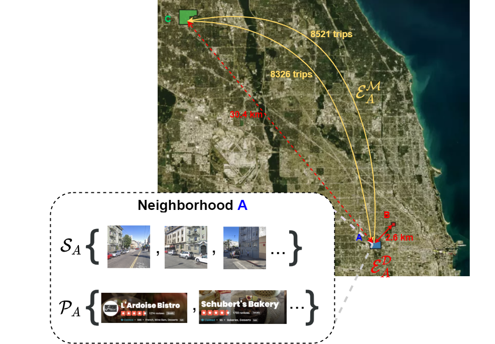
Figure 1: Multi-modal multi-graph of urban neighborhoods in the City of Chicago. Each neighborhood is a container of multi-modal inputs, e.g., street views and POIs. The neighborhoods are considered connected if they are close spatially (e.g. A and B) or or if there are many human mobility trajectories in between (e.g. A and C). Notice that even A and C are spatially far away, the large number of trips in between indicates the strong relations which should be captured in the embedding space.

The world is full of connections between entities of different modalities, such as websites and urban neighborhoods. A website can be represented as a node containing multi-modal components like text, images, and videos; hyperlinks connected websites as directed edges. Similarly, an urban neighborhood can be regarded as a complex multi-modal node containing the natural and built environment, business activities, and the people living there. Urban neighborhoods are interconnected implicitly with various types of relations such as geospatial proximity and human mobility trajectories between neighborhoods. With the vision of “smart city” being proposed in different parts of the world as well as the increasing availability of a great variety of data in cities, understanding the characteristics and dynamics of cities become essential, and more importantly, feasible with the help of state-of-the-art machine learning algorithms. Urban neighborhood embedding, or representing various urban features as vectors, is a preliminary task to many data-driven urban studies and applications such as spatiotemporal prediction, planning, and causal inference. Though abundant studies focus on representation learning for a single modality of data like images Radford et al. (2015) and text Mikolov et al. (2013), representing urban neighborhoods leveraging multi-modal data while maintaining their correlations is still a challenging task.

Traditional data collection approaches like census are costly. For example, the 2020 U.S. census was estimated to cost 15.6 billion dollars  GAO (2018). Moreover, the data produced by census is usually aggregated at pre-defined geographic divisions (e.g., census tracts and counties) and can hardly be re-mapped into other customized geospatial units such as raster tiles or polygons, which limits the flexibility of using the data. There are recent attempts to extract or predict urban characteristics from widely-available urban-associated data using data-driven approaches, including both supervised and unsupervised learning. Supervised learning methods utilize geo-tagged data such as point-of-interest (POI) Yuan et al. (2012), and street view imagery Gebru et al. (2017) as inputs and output the inference of local socioeconomic attributes. However, supervised learning is task-specific: The representation learned is not necessarily transferrable to other tasks. Furthermore, developing supervised learning models with high-dimensional data like images requires a massive dataset with annotated labels of ground-truth socioeconomic attributes, which is not necessarily available for certain regions or at the desired geographic level (e.g., raster tiles). By contrast, unsupervised learning overcomes such limitations by developing a universal and versatile representation without task-specific ground-truth supervisions. Common urban features to use include POI Fu et al. (2019), street views Law and Neira (2019), and taxi trips Yao et al. (2018). However, most of the existing unsupervised urban representation learning is still based on unimodal data, without fully leveraging various types of data both within and between neighborhoods.

Urban neighborhoods are complex systems that can be modeled by a multi-modal multi-graph: Each urban neighborhood (“node”) is a “container” which contains the built environment, business activities, and population inside the neighborhood. There are also relations (“edge”) between neighborhoods, which can be characterized by geospatial proximity, mobility connections, or both. To obtain a comprehensive representation of urban neighborhoods, we model the neighborhoods in an urban area as multi-modal multi-graph (M3G) and develop an unsupervised representation learning framework to obtain the neighborhood embedding from the graph. Instead of learning the graph globally, we propose a contrastive sampling approach that samples triplet (anchor, positive, negative) according to the multi-graph edges, enabling scalable training with multi-city data. Our major contribution is three-fold: 1) We proposed a framework to learn neighborhood representation by jointly modeling both inter- and intra-neighborhood multi-modal data as a multi-graph. 2) We demonstrate this framework with real-world data in two U.S. metropolitan areas at the census-tract level, using street view images and POI features as intra-neighborhood characteristics, and geospatial proximity and mobility flow as inter-neighborhood relations. The neighborhood embeddings generated from our framework achieve state-of-the-art performance in all downstream prediction tasks. 3) We propose three qualitative evaluations for the neighborhood embedding space, showing that our model successfully integrates various data modalities in the embedding space.

2 Related Work

2.0.1 Spatiotemporal Representation Learning

Spatiotemporal representation learning aims to produce region embedding using geo/temporal-tagged data under the First Law of Geography Tobler (1970). Chu et al. (2019); Mac Aodha et al. (2019) generate geo-aware prior based on the geo-coding of coordinates. Tile2vec Jean et al. (2019) starts the stream of imposing such prior to the embedding space through contrastive learning. Using geo-proximity as the single criterion to sample positive and negative tiles, this algorithm judiciously pushes the latter further away from the anchor point in the embedding space as compared with the former. Unfortunately, such framework can not be easily applied to multi-modal settings as a consistent and meaningful distance measure is required between any two samples across different modalities. Urban2Vec Wang et al. (2020) overcomes such drawbacks by introducing the neighborhood embedding. It is worth noticing the spatiotemporal relation between each sample can be viewed as a reciprocal relation denoted by an undirected edge. Jiang (2020) introduces the use of mobility, POI similarity or even the likeness of geo-tagged tweets Zhang et al. (2017) as new metrics of proximity to define “edges”. In this work, we generalize the contrastive learning approach to non-reciprocal relations such as mobility flow and propose a framework that can be easily extended to other graph-structured datasets with multi-modal edges and multi-modal nodes.

2.0.2 Graph Embedding

There are a lot of graph embedding methods (e.g., DeepWalk Perozzi et al. (2014), node2vec Grover and Leskovec (2016)) that generates embedding for a certain node in the graph. They can be applied to the mobility graph. For example, Fu et al. (2019) incorporate such prior by directly impose an autocorrelation in the latent space. However, most of them are not able to model multi-modal edge (as in a multi-graph), and their embedding space does not reflect the multi-perspective proximity between nodes. To further incorporate information from both nodes (e.g. POI, street view) and edges (e.g. mobility, distance), Jenkins et al. (2019) concatenate image embedding and graph embedding at each node. Our training strategy can be viewed as an extension of the contrastive sampling technique in Graph Neural Network setting (Schroff et al. (2015); Qiu et al. (2020)): By sampling triplets according to multiple proximity measures, the embedding captures the multi-graph topological properties as well as the multi-modal features from each node.

2.0.3 Urban Computing

Urban Computing aims to tackle major issues in cities, such as traffic control, public health and economic development, by modeling and analyzing urban data. A lot of research have shown the possibility to infer this socioeconomic information from satellite image Jean et al. (2016); Sheng et al. (2020), street view Gebru et al. (2017), human mobility Xu et al. (2018) and geo-tagged social network activities Schwartz and Hochman (2014). Recent studies also demonstrate that similar tasks could benefit from multi-modal inputs:  Wang et al. (2016) utilizes both POI data and taxi trip data to infer crime rate in Chicago.  Irvin et al. (2020) includes a fusion of auxiliary variables, such as elevation and air pressure, with a computer vision model on satellite images to improve the performance of forest loss driver classification. We hope the multi-graph framework proposed in this work will provide a much convenient and comprehensive tool for urban computing tasks with multi-modal data.

3 Methods

In the following section, we first mathematically define the problem of learning neighborhood embedding and give an overview of the construction of Multi-Modal Multi Graph (M3G). Then we introduce the concept of neighborhood container and our contrastive sampling strategy to incorporate multi-modal inputs at each node. We continue by describing our inter-neighborhood learning strategy for both directed and undirected edges. This section is concluded by a summary of the loss function used in M3G.

3.1 Problem Statement

Unlike most of the previous studies that focus on specific modality (e.g., image, text, etc.) and specific geographic unit (e.g. census tract, county, etc.), we restate the general problem of Urban Neighborhood Embedding agnostic to both as the following:

Definition 3.1 (Urban Neighborhood Embedding Problem).

Given a metropolitan area $\mathcal{A}$ that is composed of a set of disjointed neighborhood geometries $\mathcal{U}=\{u_{1},u_{2},...,u_{N}\}$, s.t. $\mathcal{A}=\bigcup_{i}^{N}u_{i}$, the goal of urban neighborhood embedding is to learn a vector representation $z_{i}\in\mathbb{R}^{d}$ for each $u_{i}$ which encodes the characteristics and mutual relations of $u_{i}$.

Notice $u_{i}$ can be a raster tile of certain size (commonly used in remote sensing), a census tract or a county. Under our abstraction we do not assume all $u_{i}$ are of the same geographic unit.

Geo-tagged data (i.e. data with GPS coordinates) is used to generate such embedding. Instead of categorising data by the modality, we use a more general approach of categorization based on how data is associated with the location(s):

Definition 3.2 (Geo-Tagged Point Data).

Geo-tagged point data is the kind of data characterizing one geolocation $l$:

$$\mathcal{D}^{p}_{m}=\{(x^{m},l)\}$$

is the set of geo-tagged point data with an input $x^{m}$ of modality $m$ at each geolocation. Examples of geo-tagged point data includes street views, POI check-in data and satellite images.

Definition 3.3 (Geo-Tagged Reciprocal Data).

Geo-tagged reciprocal data is the kind of data characterizing the relation between two geolocations $l_{1}$ and $l_{2}$, but it does not have a direction and the relation is reciprocal:

$$\mathcal{D}^{r}_{m}=\{(x^{m},l_{1},l_{2})\}\bigcup\{(x^{m},l_{2},l_{1})\}$$

is the set of geo-tagged reciprocal data with an input $x^{m}$ of modality $m$ between two geolocations. Examples of geo-tagged reciprocal data include spatial distance, road connectivity, and transaction volume.

Definition 3.4 (Geo-tagged Irreciprocal Data).

Geo-tagged reciprocal data is the kind of data characterizing the relation between two geolocations $l_{1}$ and $l_{2}$ with a direction:

$$\mathcal{D}^{ir}_{m}=\{(x^{m},l_{1},l_{2})\}$$

is the set of geo-tagged irreciprocal data with an input $x^{m}$ of modality $m$ between two geolocations. Examples of geo-tagged irreciprocal data include human mobility, commute time, and goods imports/exports.

The three categories of data are corresponding to the node, undirected, and directed edges in our M3G model and will be further explained in the next two sections. For now, let us assume $\mathcal{D}=\bigcup_{m,t}\mathcal{D}^{t}_{m}$ and introduce the concept of multi-modal multi-graph:

Definition 3.5 (Multi-Modal Multi-graph (M3G)).

The Multi-Modal Multi-graph $\mathcal{G}_{\mathcal{D}}(\mathcal{U},\mathcal{E})$ is a multi-graph for neighborhoods $\mathcal{U}$ and their edge set $\mathcal{E}$, characterized by the multi-modal geo-tagged dataset $\mathcal{D}$. The nodes $\mathcal{U}$ have attributes defined by all geo-tagged points data $\mathcal{D}^{p}_{m}$, which are described with more details in Section 3.2. The edges $\mathcal{E}$ are defined by all geo-tagged reciprocal/irreciprocal data $\mathcal{D}^{r}_{m}$ and $\mathcal{D}^{ir}_{m}$, which are described in Section 3.3.

3.2 Intra-Neighborhood Modalities

Despite their vast difference in data structure, both POI meta information and street view images depict the urban characteristics at specific location. In this section, we will use them as examples of Intra-Neighborhood Modalities and demonstrate how we incorporate their information into the neighborhood embedding.

3.2.1 Neighborhoods as Containers

Given a set of geo-tagged street view images $\mathcal{D}_{\mathcal{S}}^{p}=\{(x^{\mathcal{S}},l)\}$, where $s$ is an image and $l$ is its geolocation, we can easily assign each data point to the urban neighborhood $u_{i}$ it is located in:

$$\mathcal{S}_{i}=\{x^{\mathcal{S}}|(x^{\mathcal{S}},l)\in\mathcal{D}_{\mathcal{S}}^{p}\text{, s.t. }l\in u_{i}\}$$

Each $\mathcal{S}_{i}$ is a bag of street view images for neighborhood $u_{i}$.

Similarly, we can construct the feature container with the POIs $\mathcal{D}_{\mathcal{P}}^{p}=\{(x^{\mathcal{P}},l)\}$, where $p$ is a POI and $l$ is its geolocation. To represent each POI $p$, we further disassemble the textual information of $p$, which are extracted from the POI category, price, and customer reviews, into a bag of words $\{t\}$. By pooling bags of words of all POIs inside a neighborhood, we obtain the bag of POI words for each neighborhood $u_{i}$ in M3G.

$$\mathcal{P}_{i}=\{t|(x^{\mathcal{P}},l)\in\mathcal{D}_{\mathcal{P}}^{p}\text{, s.t. }t\in x^{\mathcal{P}}\text{ and }l\in u_{i}\}$$

$t$ denotes a word. We can extend this approach to incorporate other textual data such as geo-tagged social media posts.

3.2.2 Intra-Neighborhood Contrastive Learning Objective

With the node feature containers $\mathcal{S}_{i}$ and $\mathcal{P}_{i}$ constructed, we here propose our intra-neighborhood contrastive-sampling strategy: For each pass, we sample one neighborhood $u_{a}$ uniformly at random from $\mathcal{U}$, i.e. $u_{a}\overset{\text{u}}{\sim}\mathcal{U}$, as our anchor neighborhood. Then we sample one context street view image $s_{c}\overset{\text{u}}{\sim}\mathcal{S}_{a}$ and one negative street view image $s_{n}\overset{\text{u}}{\sim}\mathcal{S}_{-a}$, with $\mathcal{S}_{-a}=\bigcup_{i\neq a}\mathcal{S}_{a}$. Our proposed triplet loss Schroff et al. (2015) formulates as:

$$\mathcal{L}_{\mathcal{S}}(z_{a},s_{c},s_{n})=[M+||z_{a}-f_{\theta}(s_{c})||_{2}-||z_{a}-f_{\theta}(s_{n})||_{2}]_{+}$$ (1)

, where $[\cdot]_{+}$ is a rectifier and a positive constant $M$ is used to prevent infinitely large difference between these two distances. $z_{a}$ is the embedding vector for neighborhood $u_{a}$. $f_{\theta}(\cdot)$ is the learnable encoder for images, e.g. a convolutional neural network with parameters $\theta$.

Similarly, given a random sample $u_{a}$ from $\mathcal{U}$, we can sample POI word $t_{c}\overset{\text{u}}{\sim}\mathcal{P}_{a}$ and $t_{n}\overset{\text{u}}{\sim}\mathcal{P}_{-a}=\bigcup_{i\neq a}\mathcal{P}_{a}$ and construct the triplet loss for POI data:

$$\mathcal{L}_{\mathcal{P}}(z_{a},t_{c},t_{n})=[M+||z_{a}-g_{\phi}(t_{c})||_{2}-||z_{a}-g_{\phi}(t_{n})||_{2}]_{+}$$ (2)

The definitions of $[\cdot]_{+}$ and $M$ are the same as above. $g_{\phi}(\cdot)$ is the learnable encoder for word with parameters $\phi$.

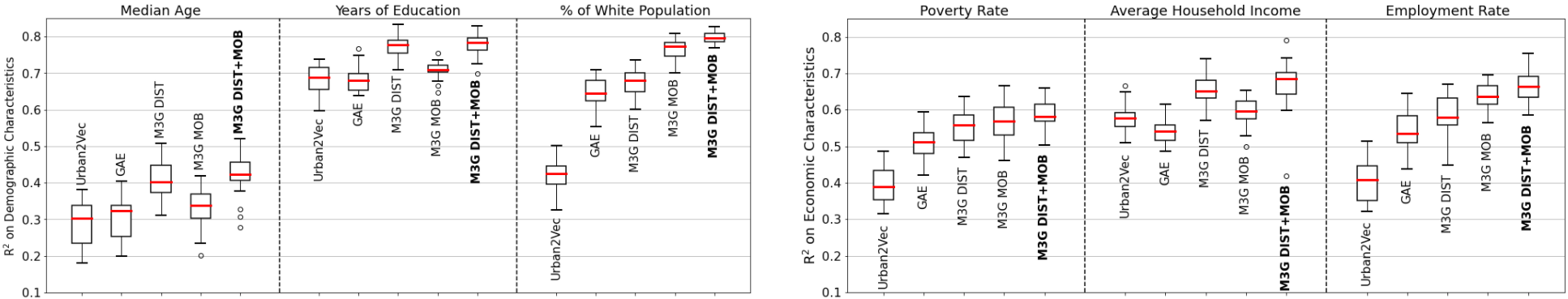
Figure 2: Prediction $R^{2}$ on neighborhood attributes with random forest model in Chicago. Left: Demographic attributes. Right: Economic attributes.

3.3 Inter-Neighborhood Modalities

Without data characterizing the relations between neighborhoods, the neighborhood embedding obtained by minimizing  (1) and (2) can only incorporate information within neighborhoods  Wang et al. (2020). In this section, we will describe how $\mathcal{D}^{r}_{j}$ and $\mathcal{D}^{ir}_{j}$ characterizes the edges in graph $\mathcal{G}$ and introduce our learning strategy for inter-neighborhood modalities. We include both spatial distance $\mathcal{D}^{r}_{\mathcal{D}}$ and human mobility $\mathcal{D}^{ir}_{\mathcal{M}}$ as examples of inter-neighborhood modalities.

3.3.1 Multi-Modal Multi-Edges

Spatial distance can be measured between any pair of neighborhoods $(u_{i},u_{j})$. We can define the outgoing edge sets of $u_{i}$ induced from the spatial distance as:

$$\mathcal{E}_{i}^{\mathcal{D}}=\{(u_{i}, u_{j},x^{\mathcal{D}})|(x^{\mathcal{D}},l_{1},l_{2})\in\mathcal{D}^{r}_{\mathcal{D}}$$

$$\text{ s.t. }l_{1}\in u_{i}\text{ and }l_{2}\in u_{j}\}$$

Here $x^{\mathcal{D}}=\frac{1}{d_{ij}}$, which is the reciprocal of geospatial distance between $u_{i}$ and $u_{j}$. Notice that $\mathcal{D}^{r}_{\mathcal{D}}$ already includes both directions of a same undirected edge according to Definition 3.4. Similarly we can define the outgoing edge sets of $u_{i}$ induced from the human mobility $\mathcal{D}^{ir}_{\mathcal{M}}$:

$$\mathcal{E}_{i}^{\mathcal{M}}=\{(u_{i}, u_{j},x^{\mathcal{M}})|(x^{\mathcal{M}},l_{1},l_{2})\in\mathcal{D}^{ir}_{\mathcal{M}}$$

$$\text{ s.t. }l_{1}\in u_{i}\text{ and }l_{2}\in u_{j}\}$$

Here $x^{\mathcal{M}}$ is the total number of trips from a geolocation in $u_{i}$ to a geolocation in $u_{j}$. Once we add both sets of edges to the graph $\mathcal{G}$, it is likely there can be multiple edges between $u_{i}$ and $u_{j}$ from different modalities.

3.3.2 Inter-Neighborhood Contrastive Learning Objectives

Like Section 3.2, we first sample one neighborhood $u_{a}$ at random from $\mathcal{U}$, i.e. $u_{a}\overset{\text{u}}{\sim}\mathcal{U}$. Instead of defining the context and negative set explicitly as in Section 3.2, we draw samples of context neighborhood by sampling each edge with the probability proportional to the weights associated with it. Specifically, edge $(u,v,w)$ has weight of $p_{m}(w)$ being sampled, with $p_{m}(\cdot)$ a designed thresholding function using the prior on modality $m$. For example, for the spatial distance, we can set

$$p_{\mathcal{S}}(w)=\begin{cases}1,\quad\text{if }w>\frac{1}{500}\\ 0,\quad\text{otherwise}\end{cases}$$

to sample a context neighborhood within a radius of 500 meters. Hence, for modality $m\in\{\mathcal{D},\mathcal{M}\}$, the probability of $u_{j}$ being sampled as a context neighborhood $u_{c}$ is:

$$P^{m}_{a,j}=\frac{\sum_{(u,v,w)\in\mathcal{E}_{a}^{m}}p_{m}(w)\mathbbm{1}_{a}(u)\mathbbm{1}_{j}(v)}{\sum_{(u,v,w)\in\mathcal{E}_{a}^{m}}p_{m}(v)\mathbbm{1}_{a}(u)}$$ (3)

Here $\mathbbm{1}_{x}(\cdot)$ is the indicator function with the value 0 everywhere except for $x$. The negative neighborhood $u_{n}$ is sampled uniformly at random from the set of rest of nodes $\{u_{j}|P_{a,j}^{m}=0\}$. Finally, we have the inter-neighborhood triplet loss for each modality $m\in\{\mathcal{D},\mathcal{M}\}$:

$$\mathcal{L}_{m}(z_{a},z_{c},z_{n})=[M+||z_{a}-z_{c}||_{2}-||z_{a}-z_{n}||_{2}]_{+}$$ (4)

The definitions of $[\cdot]_{+}$ and $M$ are the same as above. By default, we sample balanced number of triplets for each modality. Together with Equation (1) and (2), we are able to train our neighborhood embedding with any modality of inter/intra-neighborhood data. Next section will demonstrate our framework with experiments on real-world datasets.

4 Experiment

Model	Demographic characteristics			Economic characteristics
	Median age	Years of education	Percentage of white population	Poverty rate	Average household income	Employment rate
Urban2Vec Wang et al. (2020)	$0.326\pm 0.056$	$0.701\pm 0.035$	$0.472\pm 0.052$	$0.418\pm 0.052$	$0.515\pm 0.052$	$0.441\pm 0.059$
GAE Kipf and Welling (2016)	$0.261\pm 0.072$	$0.672\pm 0.024$	$0.480\pm 0.061$	$0.432\pm 0.078$	$0.457\pm 0.047$	$0.435\pm 0.079$
M3G DIST	$0.344\pm 0.052$	$0.756\pm 0.030$	$0.630\pm 0.038$	$0.488\pm 0.053$	$0.548\pm 0.047$	$0.530\pm 0.046$
M3G MOB	$0.338\pm 0.063$	$0.780\pm 0.020$	$\mathbf{0.736\pm 0.021}$	$0.591\pm 0.049$	$0.616\pm 0.029$	$0.615\pm 0.038$
M3G DIST+MOB	$\mathbf{0.374\pm 0.060}$	$\mathbf{0.790\pm 0.022}$	$0.734\pm 0.030$	$\mathbf{0.602\pm 0.049}$	$\mathbf{0.630\pm 0.038}$	$\mathbf{0.627\pm 0.036}$

Table 1: Prediction $R^{2}$ on demographic and economic attributes with linear regression model in Chicago.

To demonstrate the effectiveness of our framework, we conduct experiments on 1294 census tracts in Chicago and 1310 census tracts in New York City. We demonstrate our framework at census-tract level because the reference data for prediction (e.g., American Community Survey (ACS)) are readily available at this level. Our framework can be easily applied to other geographic divisions (e.g. block groups) or even customized units (e.g. raster tiles).

4.1 Data Description

The street view images and POI features we used are obtained from Google Street view API and Yelp Fusion API, respectively. We randomly sample 50 street views for each census tract. The human mobility data is provided by SafeGraph. Specifically, we use Core Places and Weekly Patterns datasets, which include, for each POI, the exact location, as well as the aggregated weekly estimates of the home CBGs of visitors. We preprocess the weekly patterns in Chicago and New York City from Jan 2018 to Dec 2019. Each visit is encoded as a directed edge between neighborhoods of POI and visitor’s home; both are aggregated at the census tract level. Their statistics are summarized in Table 2.

	Area ($km^{2}$)	# Edges	Average in/out degree
Chicago	$606$	$143,235$	$110$
New York City	$1212$	$120,470$	$92$

Table 2: Safegraph mobility data statistics

4.2 Training Details

For all experiments we set embedding dimension $d=200$ for images, POI words, and neighborhood. We use an Inception-v3 Szegedy et al. (2016) architecture as the encoder for street view images (i.e., $f_{\theta}(\cdot)$ in Equation (1)). The encoder for POI words(i.e., $g_{\phi}(\cdot)$ in Equation (2)) is a look-up table with weights initialized by GloVe Pennington et al. (2014). During training, we minimize loss  (1),  (2),  (4) sequentially in a three-stage process. When we sample inter-neighborhood triplet, for spatial distance, we sample $u_{c}$ uniformly at random from the $5$ closest neighbors and sample $u_{n}$ uniformly at random from the rest.

We obtain M3G neighborhood embeddings using three different configurations of edge modalities (1) Spatial distance only (M3G DIST); (2) Mobility only (M3G MOB); (3) Both spatial distance and mobility (M3G DIST+MOB). We compare the embedding with the one derived using Urban2Vec method Wang et al. (2020), which rely solely on intra-neighborhood modalities, and GAE Kipf and Welling (2016), which extract information from mobility graph using Graph Autoencoder.

5 Results and Discussion

5.1 Predicting Demographics and Economics

In this task, we treat trained neighborhood embeddings as input features to predict ACS demographic and economic attributes for each census tract. We choose Median Age, Years of Education, and Percentage of White Population as demographic attributes, and Poverty Rate, Average Household Income and Employment Rate as economic attributes. We apply PCA to reduce the embedding dimensions to 50 before running the regression model. In this work, we try both linear regression and random forest regression. Census tracts are split into training set (85%), and test set (15%). We use $R^{2}$ as the major metrics and randomly reshuffle train/test split for 20 rounds to estimate variance of the performance.

As is shown in Figure 2, two models trained with single edge modality outperform one another on different attributes: For example, for Median Age and Years of Education, M3G DIST outperforms M3G MOB, while M3G MOB has a higher average $R^{2}$ for Percentage of White Population and Employment Rate. However, by combing both modalities, M3G DIST + MOB always outperform both of them and the baseline models Urban2Vec and GAE on all demographic and economic attributes, indicating the benefits of incorporating both intra- and inter-neighborhood modalities to capture mult-perspective urban characteristics. Linear regression results from Table 1 follow a similar pattern: M3G DIST+MOB outperforms all other models on all attributes except Percentage of White Population.

5.2 Training with Multi-City Data

Since we adopt a contrastive sampling approach to learn the graph structure, we can easily scale up experiments to multiple cities without facing any memory issue. In this experiment, we investigate the improvements from training with merged data of both Chicago and New York City. Table 3 shows the mean of $R^{2}$ for predicting all 6 demographic and economic attributes using linear regression. As is shown, using multi-city training set in Chicago yields better prediction performance but not for New York City. This may be explained by the relative sparse mobility data in New York City.

Model	Training set	Test set
		Chicago	New York City
M3G MOB	Single-city	$0.613$	$0.524$
	Multi-city	$0.627$	$0.518$

Table 3: Average prediction $R^{2}$, training on single-/multi-city data.

5.3 Qualitative Analysis of the Embedding Space

5.3.1 Clustering of Neighborhood Embeddings

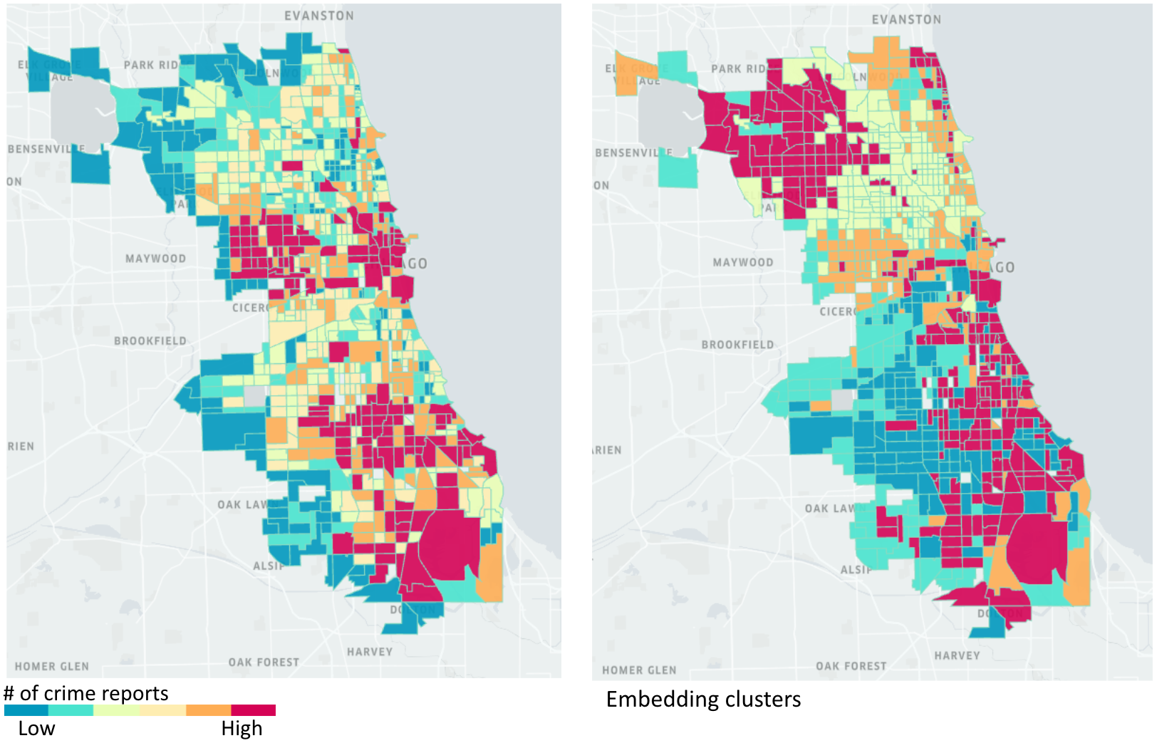
Figure 3: Color-coded map based on Left: Total number of crimes Right: Embedding clusters derived by $k$-means ($k$=6) for Chicago.

To interpret the neighborhood embeddings learned from our models, we apply $k$-means clustering on the generated embedding. Figure 3 shows the results for $k=6$ in Chicago. As the plot shows, Downtown Chicago and South Chicago, which have a high number of crime reports, are clustered into one group (red), while neighborhoods in the north like Evanston are clustered into other groups (yellow and orange).

5.3.2 Correlation with Geospatial and Mobility Proximity

In this analysis, we investigate the correlations between inter-neighborhood embedding distance and their real-world proximity in terms of geo-distance or mobility. In Figure 4, we sample 0.1% of the 1.6 M pairs of census tracts in Chicago and measure the L2 distances between their embedding vectors. With a larger number of aggregated visitors in between, neighborhoods tend to have representations closer in the embedding space; as spatial distance becomes larger, two neighborhoods tend to fall further apart in the embedding space. Such trends demonstrate that the embedding indeed captures both the geospatial and mobility relations through training.

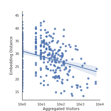
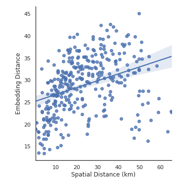
Figure 4: Correlation between geospatial/mobility proximity of node pairs in the graph and the corresponding embedding distance in Chicago. Left: The horizontal axis is the total number of visitors (bidirectional) between each pair from January 2018 to December 2019. Right: The horizontal axis is the spatial distance measured in km.

5.3.3 Neighborhood Embedding and Input Data Embedding

We are also interested in whether the neighborhood embedding incorporates information from the geo-tagged point data. We apply PCA to extract the first two principal components of the embeddings of both neighborhoods and street views and plot their distribution in Figure 5. Large points with black borders denote neighborhoods; small points denote street view images, with the color indicating the neighborhood they belong to. Here, we randomly selected three census tracts for visualization. Census tracts in Orange, Blue, and Green have average household income of $34,407, $43,836, and $113,479, respectively. As the plot shows, street view embeddings scatter around their corresponding neighborhood embedding. Though all three sampled images contain large portion of vegetation, their visual difference (e.g. trimmed or not, road landscape) can be reflected by their proximity in embedding space.

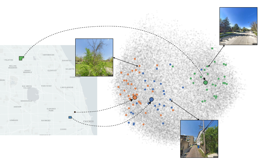
Figure 5: Positions of embeddings in the plane of the first two PCA components, for both neighborhood and street view images.

6 Conclusion

In this work, we develop M3G, a framework to model urban neighborhoods as a multi-modal multi-graph and thus learn the neighborhood representation. To demonstrate our framework, we use street view images and POIs as two modalities of data inside the neighborhood and both geospatial proximity and mobility pattern as two modalities of “edges” between neighborhoods. We show the neighborhood embedding from our framework outperforms the ones from other multi-modal models in the downstream prediction tasks while preserving both proximity/mobility connections between neighborhoods, and relations between the neighborhood and street views. The method we propose here is a general framework to learn representation for a graph with multi-modal “node” and multi-modal “edge”. Such a framework can further integrate other modalities like satellite imagery (as components of the “nodes”) and inter-region transactions (as “edges”), and even be extended to learn the representation of other graph-structured data such as websites, which will be an important task in our future work.

Model	Demographic characteristics			Economic characteristics
	Median age	Years of education	Percentage of white population	Poverty rate	Average household income	Employment rate
Urban2Vec Wang et al. [2020]	$4.081$	$0.724$	$0.186$	$0.076$	$20,270$	$0.047$
GAE Kipf and Welling [2016]	$4.283$	$0.740$	$0.182$	$0.073$	$20,531$	$0.046$
M3G DIST	$3.983$	$0.642$	$0.153$	$0.072$	$19,295$	$0.043$
M3G MOB	$3.975$	$0.600$	$\mathbf{0.128}$	$0.064$	$17,794$	$0.039$
M3G DIST+MOB	$\mathbf{3.861}$	$\mathbf{0.583}$	$0.129$	$\mathbf{0.064}$	$\mathbf{17,509}$	$\mathbf{0.038}$

Table 4: Prediction MAE on demographic and economic attributes with linear regression model in Chicago

Model	Demographic characteristics			Economic characteristics
	Median age	Years of education	Percentage of white population	Poverty rate	Average household income	Employment rate
Urban2Vec Wang et al. [2020]	$4.181$	$0.739$	$0.193$	$0.079$	$18,728$	$0.048$
GAE Kipf and Welling [2016]	$4.104$	$0.716$	$0.140$	$0.070$	$18,693$	$0.041$
M3G DIST	$3.747$	$0.608$	$0.140$	$0.064$	$16,493$	$0.039$
M3G MOB	$4.014$	$0.690$	$0.114$	$0.064$	$17,088$	$0.036$
M3G DIST+MOB	$\mathbf{3.716}$	$\mathbf{0.587}$	$\mathbf{0.064}$	$\mathbf{0.064}$	$\mathbf{15,578}$	$\mathbf{0.035}$

Table 5: Prediction MAE on demographic and economic attributes with random forest model in Chicago

Model	Demographic characteristics			Economic characteristics
	Median age	Years of education	Percentage of white population	Poverty rate	Average household income	Employment rate
Urban2Vec Wang et al. [2020]	$0.430$	$0.634$	$0.496$	$0.494$	$0.533$	$0.508$
GAE Kipf and Welling [2016]	$0.419$	$0.648$	$0.512$	$0.510$	$0.557$	$0.529$
M3G DIST	$0.453$	$0.680$	$0.572$	$0.523$	$0.580$	$0.544$
M3G MOB	$0.450$	$0.702$	$0.614$	$0.568$	$0.617$	$0.579$
M3G DIST+MOB	$\mathbf{0.472}$	$\mathbf{0.717}$	$\mathbf{0.618}$	$\mathbf{0.572}$	$\mathbf{0.627}$	$\mathbf{0.584}$

Table 6: Prediction Kendall’s $\tau$ on demographic and economic attributes with linear regression model in Chicago

Model	Demographic characteristics			Economic characteristics
	Median age	Years of education	Percentage of white population	Poverty rate	Average household income	Employment rate
Urban2Vec Wang et al. [2020]	$0.398$	$0.618$	$0.455$	$0.473$	$0.546$	$0.485$
GAE Kipf and Welling [2016]	$0.414$	$0.632$	$0.581$	$0.502$	$0.579$	$0.548$
M3G DIST	$0.487$	$0.694$	$0.603$	$0.569$	$0.619$	$0.582$
M3G MOB	$0.436$	$0.658$	$0.642$	$0.556$	$0.631$	$0.596$
M3G DIST+MOB	$\mathbf{0.493}$	$\mathbf{0.711}$	$\mathbf{0.673}$	$\mathbf{0.567}$	$\mathbf{0.648}$	$\mathbf{0.624}$

Table 7: Prediction Kendall’s $\tau$ on demographic and economic attributes with random forest model in Chicago

	# Street views	# POIs	# Neighborhoods (census tract)
Chicago	$64,739$	$38,445$	$1,294$
New York City	$67,271$	$50,697$	$1,310$

Table 8: Street views and POI data statistics

References

- Chu et al. [2019] Grace Chu, Brian Potetz, Weijun Wang, Andrew Howard, Yang Song, Fernando Brucher, Thomas Leung, and Hartwig Adam. Geo-aware networks for fine-grained recognition. In Proceedings of the IEEE International Conference on Computer Vision Workshops, pages 0–0, 2019.
- Fu et al. [2019] Yanjie Fu, Pengyang Wang, Jiadi Du, Le Wu, and Xiaolin Li. Efficient region embedding with multi-view spatial networks: A perspective of locality-constrained spatial autocorrelations. In Proceedings of the AAAI Conference on Artificial Intelligence, volume 33, pages 906–913, 2019.
- GAO [2018] GAO. Census Bureau Improved the Quality of Its Cost Estimation but Additional Steps Are Needed to Ensure Reliability, 2018. https://www.gao.gov/assets/700/693990.pdf, accessed 2021-01-16.
- Gebru et al. [2017] Timnit Gebru, Jonathan Krause, Yilun Wang, Duyun Chen, Jia Deng, Erez Lieberman Aiden, and Li Fei-Fei. Using deep learning and google street view to estimate the demographic makeup of neighborhoods across the united states. Proceedings of the National Academy of Sciences, 114(50):13108–13113, 2017.
- Grover and Leskovec [2016] Aditya Grover and Jure Leskovec. node2vec: Scalable feature learning for networks. In Proceedings of the 22nd ACM SIGKDD international conference on Knowledge discovery and data mining, pages 855–864, 2016.
- Irvin et al. [2020] Jeremy Irvin, Hao Sheng, Neel Ramachandran, Sonja Johnson-Yu, Sharon Zhou, Kyle Story, Rose Rustowicz, Cooper Elsworth, Kemen Austin, and Andrew Y Ng. Forestnet: Classifying drivers of deforestation in indonesia using deep learning on satellite imagery. In Proceedings of the Thirty-fourth Annual Conference on Neural Information Processing Systems Workshops, December 2020.
- Jean et al. [2016] Neal Jean, Marshall Burke, Michael Xie, W Matthew Davis, David B Lobell, and Stefano Ermon. Combining satellite imagery and machine learning to predict poverty. Science, 353(6301):790–794, 2016.
- Jean et al. [2019] Neal Jean, Sherrie Wang, Anshul Samar, George Azzari, David Lobell, and Stefano Ermon. Tile2vec: Unsupervised representation learning for spatially distributed data. In Proceedings of the AAAI Conference on Artificial Intelligence, volume 33, pages 3967–3974, 2019.
- Jenkins et al. [2019] Porter Jenkins, Ahmad Farag, Suhang Wang, and Zhenhui Li. Unsupervised representation learning of spatial data via multimodal embedding. In Proceedings of the 28th ACM International Conference on Information and Knowledge Management, pages 1993–2002, 2019.
- Jiang [2020] Zhe Jiang. A survey on spatial and spatiotemporal prediction methods. arXiv preprint arXiv:2012.13384, 2020.
- Kipf and Welling [2016] Thomas N. Kipf and Max Welling. Semi-supervised classification with graph convolutional networks. CoRR, abs/1609.02907, 2016.
- Law and Neira [2019] Stephen Law and Mateo Neira. An unsupervised approach to geographical knowledge discovery using street level and street network images. In Proceedings of the 3rd ACM SIGSPATIAL International Workshop on AI for Geographic Knowledge Discovery, pages 56–65, 2019.
- Mac Aodha et al. [2019] Oisin Mac Aodha, Elijah Cole, and Pietro Perona. Presence-only geographical priors for fine-grained image classification. In Proceedings of the IEEE International Conference on Computer Vision, pages 9596–9606, 2019.
- Mikolov et al. [2013] Tomas Mikolov, Kai Chen, Greg Corrado, and Jeffrey Dean. Efficient estimation of word representations in vector space. arXiv preprint arXiv:1301.3781, 2013.
- Pennington et al. [2014] Jeffrey Pennington, Richard Socher, and Christopher Manning. GloVe: Global vectors for word representation. In Proceedings of the 2014 Conference on Empirical Methods in Natural Language Processing (EMNLP), pages 1532–1543, Doha, Qatar, October 2014. Association for Computational Linguistics.
- Perozzi et al. [2014] Bryan Perozzi, Rami Al-Rfou, and Steven Skiena. Deepwalk: Online learning of social representations. In Proceedings of the 20th ACM SIGKDD international conference on Knowledge discovery and data mining, pages 701–710, 2014.
- Qiu et al. [2020] Jiezhong Qiu, Qibin Chen, Yuxiao Dong, Jing Zhang, Hongxia Yang, Ming Ding, Kuansan Wang, and Jie Tang. Gcc: Graph contrastive coding for graph neural network pre-training. In Proceedings of the 26th ACM SIGKDD International Conference on Knowledge Discovery & Data Mining, pages 1150–1160, 2020.
- Radford et al. [2015] Alec Radford, Luke Metz, and Soumith Chintala. Unsupervised representation learning with deep convolutional generative adversarial networks. arXiv preprint arXiv:1511.06434, 2015.
- Schroff et al. [2015] Florian Schroff, Dmitry Kalenichenko, and James Philbin. Facenet: A unified embedding for face recognition and clustering. In Proceedings of the IEEE conference on computer vision and pattern recognition, pages 815–823, 2015.
- Schwartz and Hochman [2014] Raz Schwartz and Nadav Hochman. The social media life of public spaces: Reading places through the lens of geo-tagged data, 2014.
- Sheng et al. [2020] Hao Sheng, Xiao Chen, Jingyi Su, Ram Rajagopal, and Andrew Ng. Effective data fusion with generalized vegetation index: Evidence from land cover segmentation in agriculture. In Proceedings of the IEEE/CVF Conference on Computer Vision and Pattern Recognition (CVPR) Workshops, June 2020.
- Szegedy et al. [2016] Christian Szegedy, Vincent Vanhoucke, Sergey Ioffe, Jon Shlens, and Zbigniew Wojna. Rethinking the inception architecture for computer vision. In Proceedings of the IEEE Conference on Computer Vision and Pattern Recognition (CVPR), June 2016.
- Tobler [1970] Waldo R Tobler. A computer movie simulating urban growth in the detroit region. Economic geography, 46(sup1):234–240, 1970.
- Wang et al. [2016] Hongjian Wang, Daniel Kifer, Corina Graif, and Zhenhui Li. Crime rate inference with big data. In Proceedings of the 22nd ACM SIGKDD international conference on knowledge discovery and data mining, pages 635–644, 2016.
- Wang et al. [2020] Zhecheng Wang, Haoyuan Li, and Ram Rajagopal. Urban2vec: Incorporating street view imagery and pois for multi-modal urban neighborhood embedding. In Proceedings of the AAAI Conference on Artificial Intelligence, volume 34, pages 1013–1020, 2020.
- Xu et al. [2018] Yang Xu, Alexander Belyi, Iva Bojic, and Carlo Ratti. Human mobility and socioeconomic status: Analysis of singapore and boston. Computers, Environment and Urban Systems, 72:51–67, 2018.
- Yao et al. [2018] Zijun Yao, Yanjie Fu, Bin Liu, Wangsu Hu, and Hui Xiong. Representing urban functions through zone embedding with human mobility patterns. In IJCAI, pages 3919–3925, 2018.
- Yuan et al. [2012] Jing Yuan, Yu Zheng, and Xing Xie. Discovering regions of different functions in a city using human mobility and pois. In Proceedings of the 18th ACM SIGKDD international conference on Knowledge discovery and data mining, pages 186–194, 2012.
- Zhang et al. [2017] Chao Zhang, Keyang Zhang, Quan Yuan, Haoruo Peng, Yu Zheng, Tim Hanratty, Shaowen Wang, and Jiawei Han. Regions, periods, activities: Uncovering urban dynamics via cross-modal representation learning. In Proceedings of the 26th International Conference on World Wide Web, pages 361–370, 2017.