CombOptNet: Fit the Right NP-Hard Problem by
Learning Integer Programming Constraints

Abstract

Bridging logical and algorithmic reasoning with modern machine learning techniques is a fundamental challenge with potentially transformative impact. On the algorithmic side, many NP-hard problems can be expressed as integer programs, in which the constraints play the role of their “combinatorial specification.” In this work, we aim to integrate integer programming solvers into neural network architectures as layers capable of learning both the cost terms and the constraints. The resulting end-to-end trainable architectures jointly extract features from raw data and solve a suitable (learned) combinatorial problem with state-of-the-art integer programming solvers. We demonstrate the potential of such layers with an extensive performance analysis on synthetic data and with a demonstration on a competitive computer vision keypoint matching benchmark.

1em {}[1]      // #1 return  save  load 

1 Introduction

It is becoming increasingly clear that to advance artificial intelligence, we need to dramatically enhance the reasoning, algorithmic, logical, and symbolic capabilities of data-driven models. Only then we can aspire to match humans in their astonishing ability to perform complicated abstract tasks such as playing chess only based on visual input. While there are decades worth of research directed at solving complicated abstract tasks from their abstract formulation, it seems very difficult to align these methods with deep learning architectures needed for processing raw inputs. Deep learning methods often struggle to implicitly acquire the abstract reasoning capabilities to solve and generalize to new tasks. Recent work has investigated more structured paradigms that have more explicit reasoning components, such as layers capable of convex optimization. In this paper, we focus on combinatorial optimization, which has been well-studied and captures nontrivial reasoning capabilities over discrete objects. Enabling its unrestrained usage in machine learning models should fundamentally enrich the set of available components.

On the technical level, the main challenge of incorporating combinatorial optimization into the model typically amounts to non-differentiability of methods that operate with discrete inputs or outputs. Three basic approaches to overcome this are to a) develop “soft” continuous versions of the discrete algorithms (Wang et al., 2019; Zanfir & Sminchisescu, 2018); b) adjust the topology of neural network architectures to express certain algorithmic behaviour (Graves et al., 2014, 2016; Battaglia et al., 2018); c) provide an informative gradient approximation for the discrete algorithm (Vlastelica et al., 2020a; Berthet et al., 2020). While the last strategy requires nontrivial theoretical considerations, it can resolve the non-differentiability in the strongest possible sense; without any compromise on the performance of the original discrete algorithm. We follow this approach.

The most successful generic approach to combinatorial optimization is integer linear programming (ILP). Integrating ILPs as building blocks of differentiable models is challenging because of the nontrivial dependency of the solution on the cost terms and on the constraints. Learning parametrized cost terms has been addressed in Vlastelica et al. (2020a); Berthet et al. (2020); Ferber et al. (2020), the learnability of constraints is, however, unexplored. At the same time, the constraints of an ILP are of critical interest due to their remarkable expressive power. Only by modifying the constraints, one can formulate a number of diverse combinatorial problems (shortest-path, matching, max-cut, Knapsack, travelling salesman). In that sense, learning ILP constraints corresponds to learning the combinatorial nature of the problem at hand.

In this paper, we propose a backward pass (gradient computation) for ILPs covering their full specification, allowing to use blackbox ILPs as combinatorial layers at any point in the architecture. This layer can jointly learn the cost terms and the constraints of the integer program, and as such it aspires to achieve universal combinatorial expressivity. We demonstrate the potential of this method on multiple tasks. First, we extensively analyze the performance on synthetic data. This includes the inverse optimization task of recovering an unknown set of constraints, and a Knapsack problem specified in plain text descriptions. Finally, we demonstrate the applicability to real-world tasks on a competitive computer vision keypoint matching benchmark.

1.1 Related Work

Learning for combinatorial optimization.

Learning methods can powerfully augment classical combinatorial optimization methods with data-driven knowledge. This includes work that learns how to solve combinatorial optimization problems to improve upon traditional solvers that are otherwise computationally expensive or intractable, e.g. by using reinforcement learning (Zhang & Dietterich, 2000; Bello et al., 2016; Khalil et al., 2017; Nazari et al., 2018), learning graph-based algorithms (Veličković et al., 2018, 2020; Wilder et al., 2019), learning to branch (Balcan et al., 2018), solving SMT formulas (Balunovic et al., 2018) and TSP instances (Kool et al., 2018). Nair et al. (2020) have recently scaled up learned MIP solvers on non-trivial production datasets. In a more general computational paradigm, Graves et al. (2014, 2016) parameterize and learn Turing machines.

Optimization-based modeling for learning.

In the other direction, optimization serves as a useful modeling paradigm to improve the applicability of machine learning models and to add domain-specific structures and priors. In the continuous setting, differentiating through optimization problems is a foundational topic as it enables optimization algorithms to be used as a layer in end-to-end trainable models (Domke, 2012; Gould et al., 2016). This approach has been recently studied in the convex setting in OptNet (Amos & Kolter, 2017) for quadratic programs, and more general cone programs in Amos (2019, Section 7.3) and Agrawal et al. (2019a, b). One use of this paradigm is to incorporate the knowledge of a downstream optimization-based task into a predictive model (Elmachtoub & Grigas, 2020; Donti et al., 2017). Extending beyond the convex setting, optimization-based modeling and differentiable optimization are used for sparse structured inference (Niculae et al., 2018), MaxSat (Wang et al., 2019), submodular optimization (Djolonga & Krause, 2017) mixed integer programming (Ferber et al., 2020), and discrete and combinational settings (Vlastelica et al., 2020a; Berthet et al., 2020). Applications of optimization-based modeling include computer vision (Rolínek et al., 2020b, a), reinforcement learning (Dalal et al., 2018; Amos & Yarats, 2020; Vlastelica et al., 2020b), game theory (Ling et al., 2018), and inverse optimization (Tan et al., 2020), and meta-learning (Bertinetto et al., 2019; Lee et al., 2019).

2 Problem description

Our goal is to incorporate an ILP as a differentiable layer in neural networks that inputs both constraints and objective coefficients and outputs the corresponding ILP solution.

Furthermore, we aim to embed ILPs in a blackbox manner: On the forward pass, we run the unmodified optimized solver, making no compromise on its performance. The task is to propose an informative gradient for the solver as it is. We never modify, relax, or soften the solver.

We assume the following form of a bounded integer program:

$$\min_{{\bm{y}}\in Y}\,{\bm{c}}\cdot{\bm{y}}\qquad\text{subject to}\qquad{\bm{A}}{\bm{y}}\leq{\bm{b}},$$ (1)

where $Y$ is a bounded subset of ${\mathbb{Z}}^{n}$, $n\in{\mathbb{N}}$, ${\bm{c}}\in\mathbb{R}^{n}$ is the cost vector, ${\bm{y}}$ are the variables, ${\bm{A}}=[{\bm{a}}_{1},\ldots,{\bm{a}}_{m}]\in\mathbb{R}^{m\times n}$ is the matrix of constraint coefficients and ${\bm{b}}\in\mathbb{R}^{m}$ is the bias term. The point at which the minimum is attained is denoted by ${\bm{y}}({\bm{A}},{\bm{b}},{\bm{c}})$.

The task at hand is to provide gradients for the mapping $({\bm{A}},{\bm{b}},{\bm{c}})\to{\bm{y}}({\bm{A}},{\bm{b}},{\bm{c}})$, in which the triple $({\bm{A}},{\bm{b}},{\bm{c}})$ is the specification of the ILP solver containing both the cost and the constraints, and ${\bm{y}}({\bm{A}},{\bm{b}},{\bm{c}})\in Y$ is the optimal solution of the instance.

Example.

The ILP formulation of the Knapsack problem can be written as

$$\max_{{\bm{y}}\in\{0,1\}^{n}}{\bm{c}}\cdot{\bm{y}}\qquad\text{subject to}\qquad{\bm{a}}\cdot{\bm{y}}\leq b,$$ (2)

where ${\bm{c}}=[c_{1},\ldots,c_{n}]\in\mathbb{R}^{n}$ are the prices of the items, ${\bm{a}}=[a_{1},\ldots,a_{n}]\in\mathbb{R}^{n}$ their weights and $b\in\mathbb{R}$ the knapsack capacity.

Similar encodings can be found for many more - often NP-hard - combinatorial optimization problems including those mentioned in the introduction. Despite the apparent difficulty of solving ILPs, modern highly optimized solvers (Gurobi Optimization, 2019; Cplex, 2009) can routinely find optimal solutions to instances with thousands of variables.

2.1 The main difficulty.

Differentiability.

Since there are finitely many available values of ${\bm{y}}$, the mapping $({\bm{A}},{\bm{b}},{\bm{c}})\to{\bm{y}}({\bm{A}},{\bm{b}},{\bm{c}})$ is piecewise constant; and as such, its true gradient is zero almost everywhere. Indeed, a small perturbation of the constraints or of the cost does typically not cause a change in the optimal ILP solution. The zero gradient has to be suitably supplemented.

Gradient surrogates w.r.t. objective coefficients ${\bm{c}}$ have been studied intensively (see e.g. Elmachtoub & Grigas, 2020; Vlastelica et al., 2020a; Ferber et al., 2020). Here, we focus on the differentiation w.r.t. constraints coefficients $({\bm{A}},{\bm{b}})$ that has been unexplored by prior works.

LP vs. ILP: Active constraints.

In the LP case, the integrality constraint on $Y$ is removed. As a result, in the typical case, the optimal solution can be written as the unique solution to a linear system determined by the set of active constraints. This captures the relationship between the constraint matrix and the optimal solution. Of course, this relationship is differentiable.

However, in the case of an ILP the concept of active constraints vanishes. There can be optimal solutions for which no constraint is tight. Providing gradients for nonactive-but-relevant constraints is the principal difficulty. The complexity of the interaction between the constraint set and the optimal solution is reflecting the NP-Hard nature of ILPs and is the reason why relying on the LP case is of little help.

3 Method

First, we reformulate the gradient problem as a descend direction task. We have to resolve an issue that the suggested gradient update ${\bm{y}}-\mathrm{d}{\bm{y}}$ to the optimal solution ${\bm{y}}$ is typically unattainable, i.e. ${\bm{y}}-\mathrm{d}{\bm{y}}$ is not a feasible integer point. Next, we generalize the concept of active constraints. We substitute the binary information “active/nonactive” by a continuous proxy based on Euclidean distance.

Descent direction.

On the backward pass, the gradient of the layers following the ILP solver is given. Our aim is to propose a direction of change to the constraints and to the cost such that the solution of the updated ILP moves towards the negated incoming gradient’s direction (i.e. the descent direction).

Denoting a loss by $L$, let ${\bm{A}}$, ${\bm{b}}$, ${\bm{c}}$ and the incoming gradient $\mathrm{d}{\bm{y}}=\partial L/\partial{\bm{y}}$ at the point ${\bm{y}}={\bm{y}}({\bm{A}},{\bm{b}},{\bm{c}})$ be given. We are asked to return a gradient corresponding to $\partial L/\partial{\bm{A}}$, $\partial L/\partial{\bm{b}}$ and $\partial L/\partial{\bm{c}}$. Our goal is to find directions $\mathrm{d}{\bm{A}}$, $\mathrm{d}{\bm{b}}$ and $\mathrm{d}{\bm{c}}$ for which the distance between the updated solution ${\bm{y}}({\bm{A}}-\mathrm{d}{\bm{A}},{\bm{b}}-\mathrm{d}{\bm{b}},{\bm{c}}-\mathrm{d}{\bm{c}})$ and the target ${\bm{y}}-\mathrm{d}{\bm{y}}$ decreases the most.

If the mapping ${\bm{y}}$ is differentiable, it leads to the correct gradients $\partial L/\partial{\bm{A}}=\partial L/\partial{\bm{y}}\cdot\partial{\bm{y}}/\partial{\bm{A}}$ (analogously for ${\bm{b}}$ and ${\bm{c}}$). See Proposition 2 in the Supplementary material, for the precise formulation and for the proof. The main advantage of this formulation is that it is meaningful even in the discrete case.

However, every ILP solution ${\bm{y}}({\bm{A}}-\mathrm{d}{\bm{A}},{\bm{b}}-\mathrm{d}{\bm{b}},{\bm{c}}-\mathrm{d}{\bm{c}})$ is restricted to integer points and its ability to approach the point ${\bm{y}}-\mathrm{d}{\bm{y}}$ is limited unless $\mathrm{d}{\bm{y}}$ is also an integer point. To achieve this, let us decompose

$$\mathrm{d}{\bm{y}}=\sum_{k=1}^{n}\lambda_{k}\Delta_{k},$$ (3)

where $\Delta_{k}\in\{-1,0,1\}^{n}$ are some integer points and $\lambda_{k}\geq 0$ are scalars. The choice of basis $\Delta_{k}$ is discussed in a separate paragraph, for now it suffices to know that every point ${\bm{y}}^{\prime}_{k}={\bm{y}}-\Delta_{k}$ is an integer point neighbour of ${\bm{y}}$ pointing in a “direction of $-\mathrm{d}{\bm{y}}$”. We then address separate problems with $\mathrm{d}{\bm{y}}$ replaced by the integer updates $\Delta_{k}$.

In other words, our goal here is to find an update on ${\bm{A}}$, ${\bm{b}}$, ${\bm{c}}$ that eventually pushes the solution closer to ${\bm{y}}-\Delta_{k}$. Staying true to linearity of the standard gradient mapping, we then aim to compose the final gradient as a linear combination of the gradients coming from the subproblems.

Constraints update.

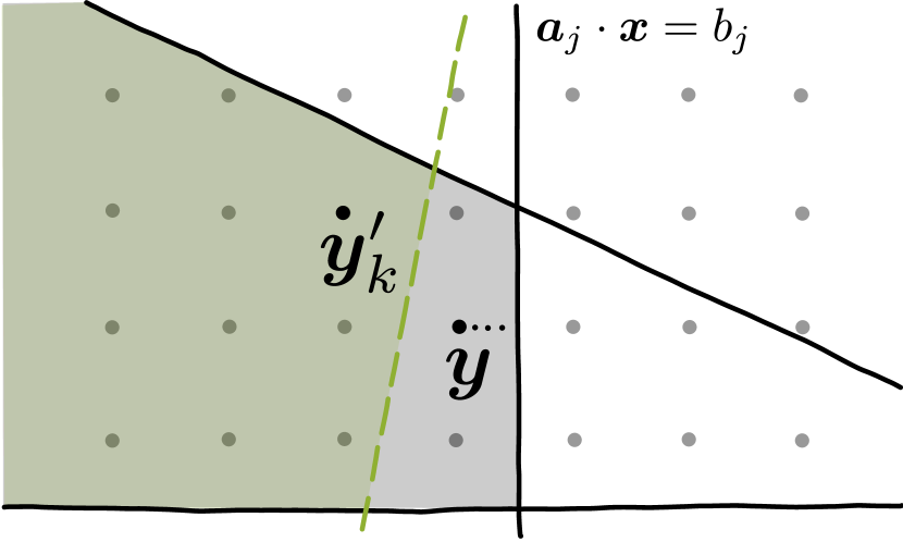
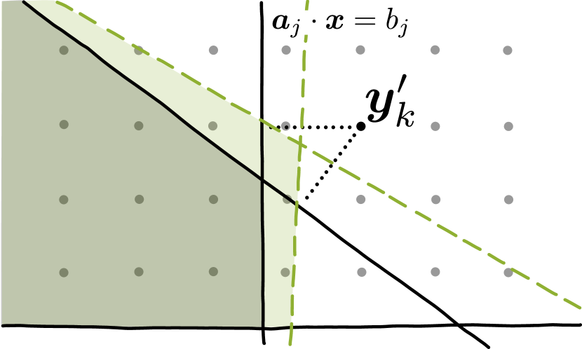
To get a meaningful update for a realizable change $\Delta_{k}$, we take a gradient of a piecewise affine local mismatch function $P_{{\bm{y}}^{\prime}_{k}}$. The definition of $P_{{\bm{y}}^{\prime}_{k}}$ is based on a geometric understanding of the underlying structure. To that end, we rely on the Euclidean distance between a point and a hyperplane. Indeed, for any point ${\bm{y}}$ and a given hyperplane, parametrized by vector ${\bm{a}}$ and scalar $b$ as ${\bm{x}}\mapsto{\bm{a}}\cdot{\bm{x}}-b$, we have:

$$\operatorname{\mathrm{dist}}({\bm{a}},b;{\bm{y}})=|{\bm{a}}\cdot{\bm{y}}-b|/\|{\bm{a}}\|.$$ (4)

Now, we distinguish the cases based on whether ${\bm{y}}^{\prime}_{k}$ is feasible, i.e. ${\bm{A}}{\bm{y}}^{\prime}_{k}\leq{\bm{b}}$, or not. The infeasibility of ${\bm{y}}^{\prime}_{k}$ can be caused by one or more constraints. We then define

$$P_{{\bm{y}}^{\prime}_{k}}({\bm{A}},{\bm{b}})=\begin{cases}\min_{j}\operatorname{\mathrm{dist}}({\bm{a}}_{j},b_{j};{\bm{y}})\\ \hskip 20.00003pt\text{\color[rgb]{0.297,0.348,0.105}\definecolor[named]{pgfstrokecolor}{rgb}{0.297,0.348,0.105}if ${\bm{y}}^{\prime}_{k}$ is feasible and ${\bm{y}}^{\prime}_{k}\neq{\bm{y}}$}\\ \sum_{j}\llbracket{\bm{a}}_{j}\cdot{\bm{y}}^{\prime}_{k}>b_{j}\rrbracket\operatorname{\mathrm{dist}}({\bm{a}}_{j},b_{j};{\bm{y}}^{\prime}_{k})\\ \hskip 20.00003pt\text{\color[rgb]{0.297,0.348,0.105}\definecolor[named]{pgfstrokecolor}{rgb}{0.297,0.348,0.105}if ${\bm{y}}^{\prime}_{k}$ is infeasible}\\ \makebox[20.00003pt][l]{0}\text{\color[rgb]{0.297,0.348,0.105}\definecolor[named]{pgfstrokecolor}{rgb}{0.297,0.348,0.105} if ${\bm{y}}^{\prime}_{k}={\bm{y}}$ or ${\bm{y}}^{\prime}_{k}\notin Y$},\end{cases}$$ (5)

where $\llbracket\cdot\rrbracket$ is the Iverson bracket. The geometric intuition behind the suggested mismatch function is described in Fig. 2 and its caption. Note that tighter constraints contribute more to $P_{{\bm{y}}^{\prime}_{k}}$. In this sense, the mismatch function generalizes the concept of active constraints. In practice, the minimum is softened to allow multiple constraints to be updated simultaneously. For details, see the Supplementary material.

(a) ${\bm{y}}^{\prime}_{k}$ is feasible but ${\bm{y}}^{\prime}_{k}\neq{\bm{y}}$.

(b) ${\bm{y}}^{\prime}_{k}$ is infeasible.

Figure 2: Geometric interpretation of the suggested constraint update. (a) All constraints are satisfied for ${\bm{y}}^{\prime}_{k}$. The proxy minimizes the distance to the nearest (“most active”) constraint to make ${\bm{y}}$ “less feasible”. A possible updated feasible region is shown in green. (b) The suggested ${\bm{y}}^{\prime}_{k}$ satisfies one of three constraints. The proxy minimizes the distance to violated constraints to make ${\bm{y}}^{\prime}_{k}$ “more feasible”.

Imposing linearity and using decomposition (3), we define the outcoming gradient $\mathrm{d}{\bm{A}}$ as

$$\mathrm{d}{\bm{A}}=\sum_{k=1}^{n}\lambda_{k}\frac{\partial P_{{\bm{y}}^{\prime}_{k}}}{\partial{\bm{A}}}({\bm{A}},{\bm{b}})$$ (6)

and analogously for $\mathrm{d}{\bm{b}}$, by differentiating with respect to ${\bm{b}}$. The computation is summarized in Module 1.

ForwardPass${\bm{A}},{\bm{b}},{\bm{c}}$${\bm{y}}:=$Solver(${\bm{A}},{\bm{b}},{\bm{c}}$) ${\bm{y}}$and ${\bm{A}},{\bm{b}},{\bm{c}}$for backward pass ${\bm{y}}$BackwardPass$\mathrm{d}{\bm{y}}$${\bm{y}}$and ${\bm{A}},{\bm{b}},{\bm{c}}$from forward pass Decompose $\mathrm{d}{\bm{y}}=\sum_{k}\lambda_{k}\Delta_{k}$set $\Delta_{k}$as in (9) and $\lambda_{k}$as in Proposition 1Calculate the gradients   $\mathrm{d}{\bm{A}}^{k}:=\frac{\partial P_{{\bm{y}}^{\prime}_{k}}}{\partial{\bm{A}}}$, $\mathrm{d}{\bm{b}}^{k}:=\frac{\partial P_{{\bm{y}}^{\prime}_{k}}}{\partial{\bm{b}}}$, $\mathrm{d}{\bm{c}}^{k}:=\frac{\partial P_{{\bm{y}}^{\prime}_{k}}}{\partial{\bm{c}}}$$P_{{\bm{y}}^{\prime}_{k}}$defined in (5) and () Compose $\mathrm{d}{\bm{A}},\mathrm{d}{\bm{b}},\mathrm{d}{\bm{c}}:=\sum_{k}\lambda_{k}\left(\mathrm{d}{\bm{A}}^{k},\mathrm{d}{\bm{b}}^{k},\mathrm{d}{\bm{c}}^{k}\right)$According to () $\mathrm{d}{\bm{A}},\mathrm{d}{\bm{b}},\mathrm{d}{\bm{c}}$

Module 1 CombOptNet

Note that our mapping $\mathrm{d}{\bm{y}}\mapsto\mathrm{d}{\bm{A}},\mathrm{d}{\bm{b}}$ is homogeneous. It is due to the fact that the whole situation is rescaled to one case (choice of basis) where the gradient is computed and then rescaled back (scalars $\lambda_{k}$). The most natural scale agrees with the situation when the “targets” ${\bm{y}}^{\prime}_{k}$ are the closest integer neighbors. This ensures that the situation does not collapse to a trivial solution (zero gradient) and, simultaneously, that we do not interfere with very distant values of ${\bm{y}}$.

This basis selection plays a role of a “homogenizing hyperparamter” ($\lambda$ in (Vlastelica et al., 2020a) or $\varepsilon$ in (Berthet et al., 2020)). In our case, we explicitly construct a correct basis and do not need to optimize any additional hyperparameter.

Cost update.

Putting aside distinguishing of feasible and infeasible ${\bm{y}}^{\prime}_{k}$, the cost update problem has been addressed in multiple previous works. We use a simple approach of setting the mismatch function such that the resulting update favours ${\bm{y}}^{\prime}_{k}$ over ${\bm{y}}$ in the updated optimization problem, i.e.

$$P_{{\bm{y}}^{\prime}_{k}}({\bm{c}})=\begin{cases}{\bm{c}}\cdot({\bm{y}}^{\prime}_{k}-{\bm{y}})\quad\text{\color[rgb]{0.297,0.348,0.105}\definecolor[named]{pgfstrokecolor}{rgb}{0.297,0.348,0.105}if ${\bm{y}}^{\prime}_{k}$ is feasible}\\ 0\hskip 28.99997pt\text{\color[rgb]{0.297,0.348,0.105}\definecolor[named]{pgfstrokecolor}{rgb}{0.297,0.348,0.105}if ${\bm{y}}^{\prime}_{k}$ is infeasible or ${\bm{y}}^{\prime}_{k}\notin Y$.}\end{cases}$$ (7)

The gradient $\mathrm{d}{\bm{c}}$ is then composed analogously as in (6).

The choice of the basis.

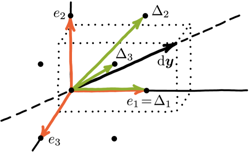
Denote by $k_{1},\ldots,k_{n}$ the indices of the coordinates in the absolute values of $\mathrm{d}{\bm{y}}$ in decreasing order, i.e.

$$|\mathrm{d}{\bm{y}}_{k_{1}}|\geq|\mathrm{d}{\bm{y}}_{k_{2}}|\geq\cdots\geq|\mathrm{d}{\bm{y}}_{k_{n}}|$$ (8)

and set

$$\Delta_{k}=\sum_{j=1}^{k}\operatorname{sign}(\mathrm{d}{\bm{y}}_{k_{j}}){\bm{e}}_{k_{j}},$$ (9)

where ${\bm{e}}_{k}$ is the $k$-th canonical vector. Therefore, $\Delta_{k}$ is the (signed) indicator vector of the first $k$ dominant directions.

Denote by $\ell$ the largest index for which $|\mathrm{d}{\bm{y}}_{\ell}|>0$. Then the first $\ell$ vectors $\Delta_{k}$’s are linearly independent and they form a basis of the corresponding subspace. Therefore, there exist scalars $\lambda_{k}$’s satisfying decomposition (3).

Proposition 1.

If $\lambda_{j}=|\mathrm{d}{\bm{y}}_{k_{j}}|-|\mathrm{d}{\bm{y}}_{k_{j+1}}|$ for $j=1,\ldots,n-1$ and $\lambda_{n}=|\mathrm{d}{\bm{y}}_{k_{n}}|$, then representation (3) holds with $\Delta_{k}$’s as in (9).

An example of a decomposition is shown in Fig. 3. Further discussion about the choice of basis and various comparisons can be found in the Supplementary material.

Figure 3: All basis vectors $\Delta_{k}$ (green) point more “towards the $\mathrm{d}{\bm{y}}$ direction” compared to the canonical ones (orange).

Constraint parametrization.

For learning constraints, we have to specify their parametrization. The representation is of great importance, as it determines how the constraints respond to incoming gradients. Additionally, it affects the meaning of constraint distance by changing the parameter space.

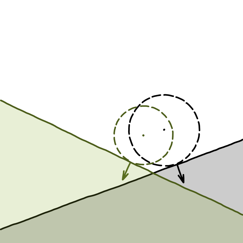
We represent each constraint $({\bm{a}}_{k},b_{k})$ as a hyperplane described by its normal vector ${\bm{a}}_{k}$, distance from the origin $r_{k}$ and offset $o_{k}$ of the origin in the global coordinate system as displayed in Fig. 4(a). Consequently $b_{k}=r_{k}-{\bm{a}}_{k}\cdot o_{k}$.

Compared to the plain parametrization which represents the constraints as a matrix ${\bm{A}}$ and a vector ${\bm{b}}$, our slightly overparametrized choice allows the constraints to rotate without requiring to traverse large distance in parameter space (consider e.g. a $180^{\circ}$ rotation). An illustration is displayed in Fig. 4(b). Comparison of our choice of parametrization to other encodings and its effect on the performance can be found in the Supplementary material.

(a) Constraint representation

(b) Possible constraint update

Figure 4: (a) Each constraint $({\bm{a}}_{k},b_{k})$ is parametrized by its normal vector ${\bm{a}}_{k}$ and a distance $r_{k}$ to its own origin $o_{k}$. (b) Such a representation allows for easy rotations around the learnable offset $o_{k}$ instead of rotating around the static global origin.

4 Demonstration & Analysis

We demonstrate the potential and flexibility of our method on four tasks.

Starting with an extensive performance analysis on synthetic data, we first demonstrate the ability to learn multiple constraints simultaneously. For this, we learn a static set of randomly initialized constraints from solved instances, while using access to the ground-truth cost vector ${\bm{c}}$.

Additionally, we show that the performance of our method on the synthetic datasets also translates to real classes of ILPs. For this we consider a similarly structured task as before, but use the NP-complete WSC problem to generate the dataset.

Next, we showcase the ability to simultaneously learn the full ILP specification. For this, we learn a single input-dependent constraint and the cost vector jointly from the ground truth solutions of knapsack instances. These instances are encoded as sentence embeddings of their description in natural language.

Finally, we demonstrate that our method is also applicable to real-world problems. On the task of keypoint matching, we show that our method achieves results that are comparable to state-of-the-art architectures employing dedicated solvers. In this example, we jointly learn a static set of constraints and the cost vector from ground-truth matchings.

In all demonstrations, we use Gurobi (Gurobi Optimization, 2019) to solve the ILPs during training and evaluation. Implementation details, a runtime analysis and additional results, such as ablations, other loss functions and more metrics, are provided in the Supplementary material. Additionally, a qualitative analysis of the results for the Knapsack demonstration is included.

4.1 Random Constraints

Problem formulation.

The task is to learn the constraints $({\bm{A}},{\bm{b}})$ corresponding to a fixed ILP. The network has only access to the cost vectors ${\bm{c}}$ and the ground-truth ILP solutions ${\bm{y}}^{*}$. Note that the set of constraints perfectly explaining the data does not need to be unique.

Dataset.

We generate 10 datasets for each cardinality $m=1,2,4,8$ of the ground-truth constraint set while keeping the dimensionality of the ILP fixed to $n=16$. Each dataset fixes a set of (randomly chosen) constraints $({\bm{A}},{\bm{b}})$ specifying the ground-truth feasible region of an ILP solver. For the constraints $({\bm{A}},{\bm{b}})$ we then randomly sample cost vectors ${\bm{c}}$ and compute the corresponding ILP solution ${\bm{y}}^{*}$ (Fig. 5).

Figure 5: Dataset generation for the RC demonstration.

The dataset consists of 1 600 pairs $({\bm{c}},{\bm{y}}^{*})$ for training and 1 000 for testing. The solution space $Y$ is either constrained to $[-5,5]^{n}$ (dense) or $[0,1]^{n}$ (binary). During dataset generation, we performed a suitable rescaling to ensure a sufficiently large set of feasible solutions.

Architecture.

The network learns the constraints $({\bm{A}},{\bm{b}})$ that specify the ILP solver from ground-truth pairs $({\bm{c}},{\bm{y}}^{*})$. Given ${\bm{c}}$, predicted solution ${\bm{y}}$ is compared to ${\bm{y}}^{*}$ via the MSE loss and the gradient is backpropagated to the learnable constraints using CombOptNet (Fig. 6).

Figure 6: Architecture design for the RC demonstration.

The number of learned constraints matches the number of constraints used for the dataset generation. Note that if the ILP has no feasible solution, the CombOptNet layer output is undefined and any loss or evaluation metric depending on the solution ${\bm{y}}$ is meaningless. In practise, updates (5) push the constraints outwards from the true solution ${\bm{y}}^{*}$ leading to a quick emergence of a feasible region.

Baselines.

We compare CombOptNet to three baselines. Agnostic to any constraints, a simple MLP baseline directly predicts the solution from the input cost vector as the integer-rounded output of a neural network. The CVXPY baseline uses an architecture similar to ours, only the Module 1 of CombOptNet is replaced with the CVXPY implementation (Diamond & Boyd, 2016) of an LP solver that provides a backward pass proposed by Agrawal et al. (2019a). Similar to our method, it receives constraints and a cost vector and outputs the solution of the LP solver greedily rounded to a feasible integer solution. Finally, we report the performance of always producing the solution of the problem only constrained to the outer region ${\bm{y}}\in Y$. This baseline does not involve any training and is purely determined by the dataset.

Results.

The results are reported in Fig. 7.

(a) Results on the binary datasets.

(b) Results on the dense datasets.

Figure 7: Results for the Random Constraints demonstration. We report mean accuracy (${\bm{y}}={\bm{y}}^{*}$ in %) over 10 datasets for $1,2,4$ and $8$ ground truth constraints in $16$ dimensions. By Box-constrained we denote the performance of always producing the solution of the problem only constrained to the outer region ${\bm{y}}\in Y$, which does not involve any training and is purely determined by the dataset.

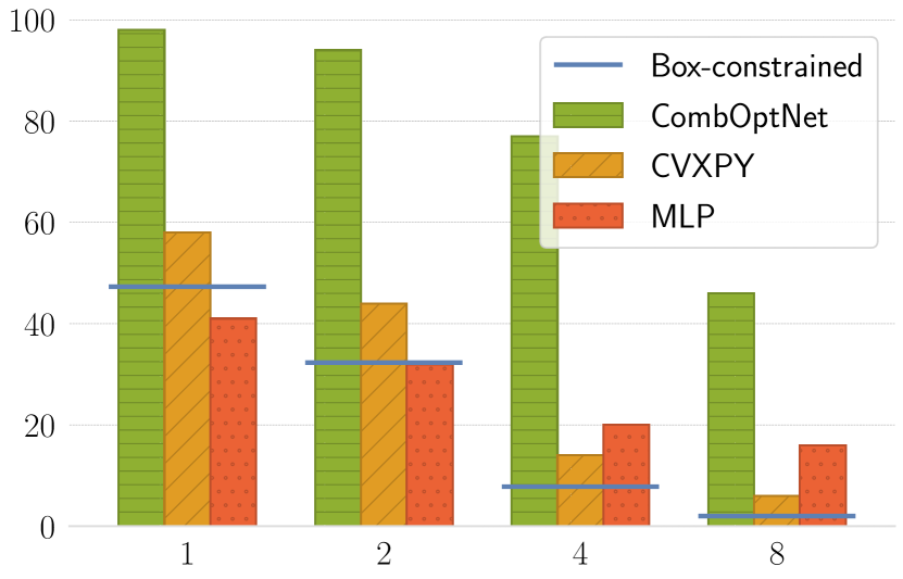
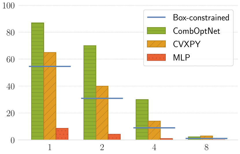
In the binary, case we demonstrate a high accuracy of perfectly predicting the correct solution. The CVXPY baseline is not capable of matching this, as it is not able to find a set of constraints for the LP problem that mimics the effect of running an ILP solver. For most cost vectors, CVXPY often predicts the same solution as the unconstrained one and its ability to use constraints to improve is marginal. The reason is that the LP relaxation of the ground truth problem is far from tight and thus the LP solver proposes many fractional solutions, which are likely to be rounded incorrectly. This highlights the increased expressivity of the ILP formulation compared to the LP formulation.

Even though all methods decrease in performance in the dense case as the number of possible solutions is increased, the trend from the binary case continues. With the increased density of the solution space, the LP relaxation becomes more similar to the ground truth ILP and hence the gap between CombOptNet and the CVXPY baseline decreases.

We conclude that CombOptNet is especially useful, when the underlying problem is truly difficult (i.e. hard to approximate by an LP). This is not surprising, as CombOptNet introduces structural priors into the network that are designed for hard combinatorial problems.

4.2 Weighted Set Covering

We show that our performance on the synthetic datasets also translates to traditional classes of ILPs. Considering a similarly structured architecture as in the previous section, we generate the dataset by solving instances of the NP-complete WSC problem.

Problem formulation.

A family $\mathcal{C}$ of subsets of a universe $U$ is called a covering of $U$ if $\bigcup\mathcal{C}=U$. Given $U=\{1,\ldots,m\}$, its covering $\mathcal{C}=\{S_{1},\ldots,S_{n}\}$ and cost ${\bm{c}}\colon\mathcal{C}\to\mathbb{R}$, the task is to find the sub-covering $\mathcal{C}^{\prime}\subset\mathcal{C}$ with the lowest total cost $\sum_{S\in\mathcal{C}^{\prime}}{\bm{c}}(S)$.

The ILP formulation of this problem consists of $m$ constraints in $n$ dimensions. Namely, if ${\bm{y}}\in\{0,1\}^{n}$ denotes an indicator vector of the sets in $\mathcal{C}$, $a_{kj}=\llbracket k\in S_{j}\rrbracket$ and $b_{k}=1$ for $k=1,\ldots m$, then the specification reads as

$$\min_{{\bm{y}}\in Y}\,\sum_{j}{\bm{c}}(S_{j}){\bm{y}}_{j}\qquad\text{subject to}\qquad{\bm{A}}{\bm{y}}\geq{\bm{b}}.$$ (10)

Dataset.

We randomly draw $n$ subsets from the $m$-element universe to form a covering $\mathcal{C}$. To increase the variance of solutions, we only allow subsets with no more than 3 elements. As for the Random Constraints demonstration, the dataset consists of 1 600 pairs $({\bm{c}},{\bm{y}}^{*})$ for training and 1 000 for testing. Here, ${\bm{c}}$ is uniformly sampled positive cost vector and ${\bm{y}}^{*}$ denotes the corresponding optimal solution (Fig. 8). We generate 10 datasets for each universe size $m=4,5,6,7,8$ with $n=2m$ subsets.

Figure 8: Dataset generation for the WSC demonstration.

Architecture and Baselines.

We use the same architecture and compare to the same baselines as in the Random Constraints demonstration (Sec. 4.1).

Results.

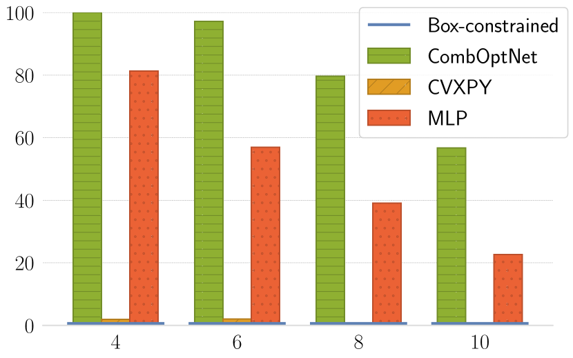
The results are reported in Fig. 9. Our method is still able to predict the correct solution with high accuracy. Compared to the previous demonstration, the performance of the LP relaxation deteriorates. Contrary to the Random Constraints datasets, the solution to the Weighted Set Covering problem never matches the solution of the unconstrained problem, which takes no subset. This prevents the LP relaxation from exploiting these simple solutions and ultimately leads to a performance drop. On the other hand, the MLP baseline benefits from the enforced positivity of the cost vector, which leads to an overall reduced number of different solutions in the dataset.

Figure 9: Results of the WSC demonstration. We report mean accuracy (${\bm{y}}={\bm{y}}^{*}$ in %) over 10 datasets for universe sizes $m=4,6,8,10$ and $2m$ subsets.

4.3 Knapsack from Sentence Description

Problem formulation.

The task is inspired by a vintage text-based PC game called “The Knapsack Problem” (Richardson, 2001) in which a collection of 10 items is presented to a player including their prices and weights. The player’s goal is to maximize the total price of selected items without exceeding the fixed 100-pound capacity of their knapsack. The aim is to solve instances of the NP-Hard Knapsack problem (Example), from their word descriptions. Here, the cost ${\bm{c}}$ and the constraint $({\bm{a}},b)$ are learned simultaneously.

Dataset.

Similarly to the game, a Knapsack instance consists of 10 sentences, each describing one item. The sentences are preprocessed via the sentence embedding (Conneau et al., 2017) and the 10 resulting 4 096-dimensional vectors ${\bm{x}}$ constitute the input of the dataset. We rely on the ability of natural language embedding models to capture numerical values, as the other words in the sentence are uncorrelated with them (see an analysis of Wallace et al. (2019)). The indicator vector ${\bm{y}}^{*}$ of the optimal solution (i.e. item selection) to a knapsack instance is its corresponding label (Fig. 10). The dataset contains 4 500 training and 500 test pairs $({\bm{x}},{\bm{y}}^{*})$.

Figure 10: Dataset generation for the Knapsack problem.

Architecture.

We simultaneously extract the learnable constraint coefficients $({\bm{a}},{\bm{b}})$ and the cost vector ${\bm{c}}$ via an MLP from the embedding vectors (Fig. 11).

Figure 11: Architecture design for the Knapsack problem.

As only a single learnable constraint is used, which by definition defines a Knapsack problem, the interpretation of this demonstration is a bit different from the other demonstrations. Instead of learning the type of combinatorial problem, we learn which exact Knapsack problem in terms of item-weights and knapsack capacity needs to be solved.

Baselines.

We compare to the same baselines as in the Random Constraints demonstration (Sec. 4.1).

Results.

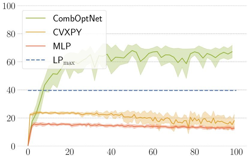
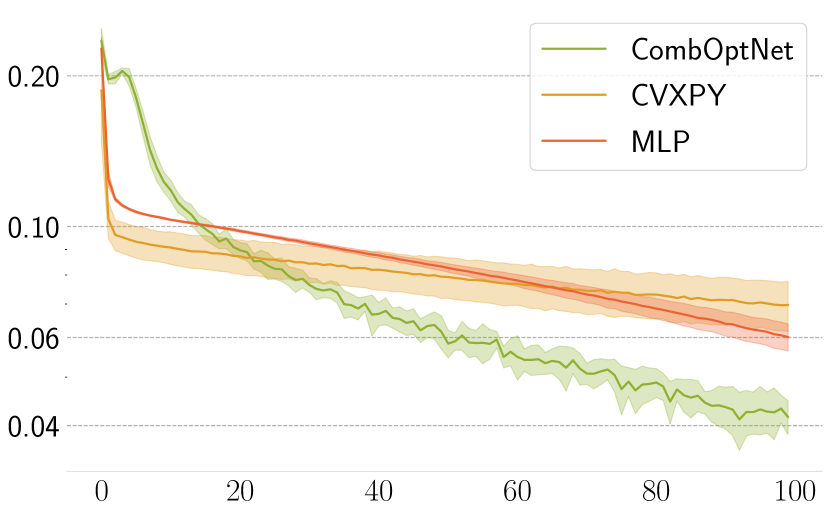
The results are presented in Fig. 12. While CombOptNet is able to predict the correct items for the Knapsack with good accuracy, the baselines are unable to match this. Additionally, we evaluate the LP relaxation on the ground truth weights and prices, providing an upper bound for results achievable by any method relying on an LP relaxation. The weak performance of this evaluation underlines the NP-Hardness of Knapsack. The ability to embed and differentiate through a dedicated ILP solver leads to surpassing this threshold even when learning from imperfect raw inputs.

(a) Evaluation accuracy (${\bm{y}}={\bm{y}}^{*}$ in %) over training epochs. LP_max is the maximum achievable LP relaxation accuracy.

(b) Training MSE loss over epochs.

Figure 12: Results or Knapsack demonstration. Reported error bars are over 10 restarts.

4.4 Deep Keypoint Matching

Problem formulation.

Given are a source and target image showing an object of the same class (e.g. airplane), each labeled with a set of annotated keypoints (e.g. left wing). The task is to find the correct matching between the sets of keypoints from visual information without access to the keypoint annotation. As not every keypoint has to be visible in both images, some keypoints can also remain unmatched.

As in this task the combinatorial problem is known a priori, state-of-the-art methods are able to exploit this knowledge by using dedicated solvers. However, we make the problem harder by omitting this knowledge. Instead, we simultaneously infer the problem specification and train the feature extractor for the cost vector from data end-to-end.

Dataset.

We use the SPair-71k dataset (Min et al., 2019) which was published in the context of dense image matching and was used as a benchmark for keypoint matching in recent literature (Rolínek et al., 2020b). It includes 70 958 image pairs prepared from Pascal VOC 2012 and Pascal 3D+ with rich pair-level keypoint annotations. The dataset is split into 53 340 training pairs, 5 384 validation pairs and 12 234 pairs for testing.

Table 1: Results for the keypoint matching demonstration. Reported is the standard per-variable accuracy $(\%)$ metric over 5 restarts. Column $p\times p$ corresponds to matching $p$ source keypoints to $p$ target keypoints. Original BB-GM has access to unary and quadratic costs; we also report performance with access only to unary costs as in CombOptNet.

Method	$4\times 4$	$5\times 5$	$6\times 6$	$7\times 7$
CombOptNet	$83.1$	$80.7$	$78.6$	$76.1$
BB-GM (unary only)	$84.3$	$81.6$	$79.0$	$76.5$
BB-GM (unary & quad.)	$84.3$	$82.9$	$80.5$	$79.8$

State-of-the-art.

We compare to a state-of-the-art architecture BB-GM (Rolínek et al., 2020b) that employs a dedicated solver for the quadratic assignment problem. Given a pair of images and their corresponding sets of keypoint locations, the method constructs for each image a graph with the nodes corresponding to the keypoints. A network then predicts the unary and quadratic costs for matching the nodes and edges between the two graphs. A heavily optimized solver for the quadratic assignment problem then computes a consistent matching of the nodes. When training the architecture, the incoming gradient is backpropagated through the solver to the unary and quadratic costs via blackbox backpropagation (Vlastelica et al., 2020a).

Architecture.

We modify the BB-GM architecture by replacing the blackbox backpropagation module employing the dedicated solver with CombOptNet.

The drop-in replacement comes with a few important considerations. Note that our method relies on a fixed dimensionality $n$ of the problem for learning a static (i.e. not input-dependent) constraint set. However, in the BB-GM architecture the dimensionality of the predicted costs depends on the number of nodes (i.e. keypoints) $p$ and number of edges in each of the two matched graphs. As these quantities vary over the dataset, the dimensionality varies as well. To avoid these issues, we resort to a simplified setting.

First, we fix the number of keypoints in both images. For each $p=4,5,6,7$, we generate an augmented dataset by randomly removing additional keypoints in images with more than $p$ keypoints. The images with fewer keypoints than $p$ are dropped. Note that even for a fixed number of keypoints the number of edges (and hence the quadratic cost dimensionality) can vary. Therefore, we omit the quadratic costs as an input to the ILP solver.

These simplifications result in a fixed ILP dimensionality of $n=p^{2}$. The number of learnable constraints coincides with the number of constraints in the corresponding unary assignment problem, i.e. the combined number of keypoints in both images $(m=2p)$.

The randomly initialized constraint set and the backbone architecture that produces the cost vectors are learned simultaneously from pairs of predicted solutions and ground-truth matchings using CombOptNet.

Results.

We report two results for the BB-GM architecture depending on the information available to the solver. In the unary setting, the solver utilizes only unary costs, in the quadratic setting, it utilizes both unary and quadratic costs. The ILP solver is restricted to the unary setting.

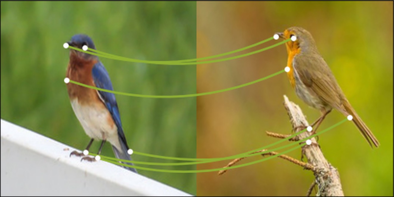
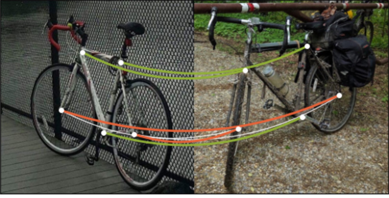
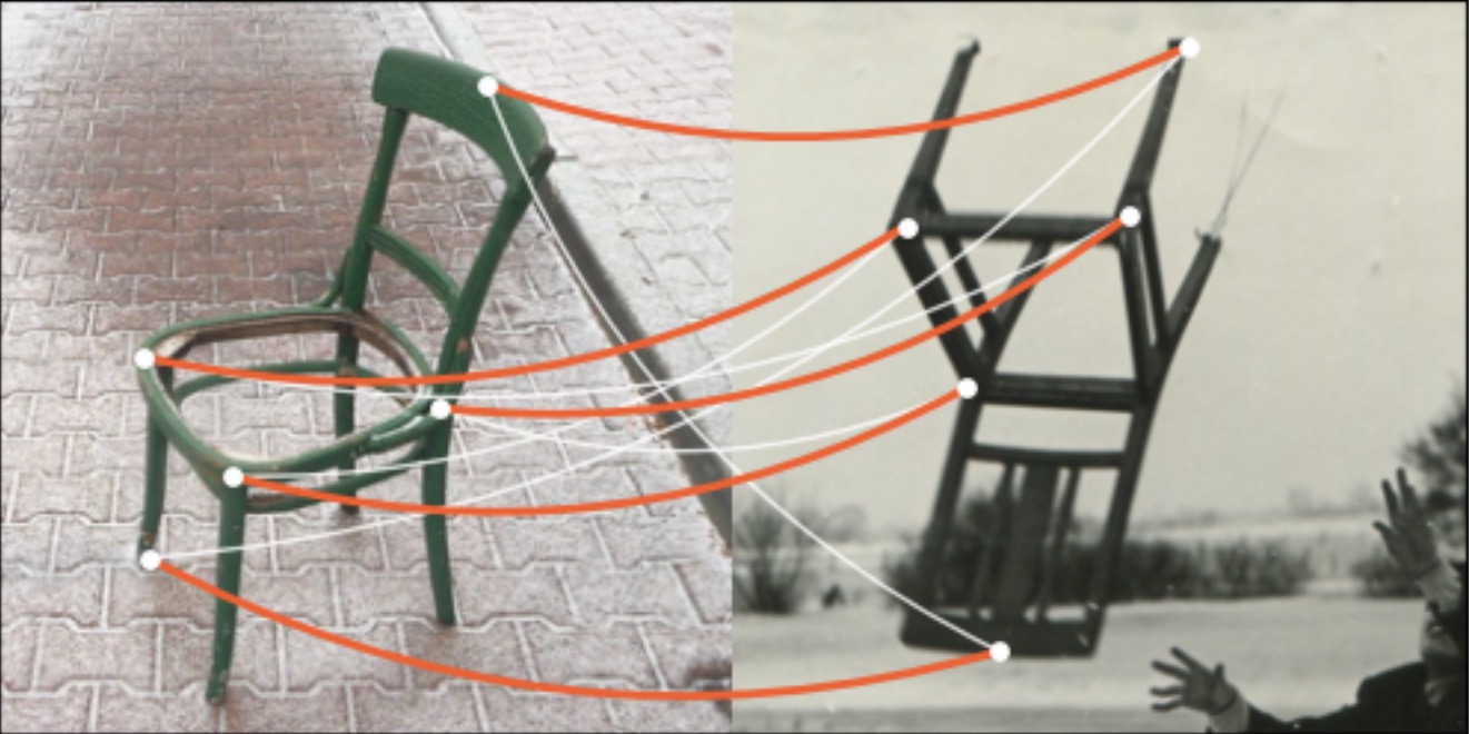
Even though the task-agnostic CombOptNet is uninformed about the underlying combinatorial problem, its performance is very close to the privileged state-of-the-art method BB-GM, especially when BB-GM is restricted to use the same information (unary costs only). These results are especially satisfactory, considering that BB-GM outperforms the previous state-of-the-art architecture (Fey et al., 2020) by several percentage points on experiments of this difficulty. Example matchings are shown in Fig. 13.

Figure 13: Example matchings predicted by CombOptNet.

5 Conclusion

We propose a method for integrating integer linear program solvers into neural network architectures as layers. This is enabled by providing gradients for both the cost terms and the constraints of an ILP. The resulting end-to-end trainable architectures are able to simultaneously extract features from raw data and learn a suitable set of constraints that specify the combinatorial problem. Thus, the architecture learns to fit the right NP-hard problem needed to solve the task. In that sense, it strives to achieve universal combinatorial expressivity in deep networks—opening many exciting perspectives.

In the experiments, we demonstrate the flexibility of our approach, using different input domains, natural language and images, and different combinatorial problems with the same CombOptNet module. In particular, for combinatorially hard problems we see a strong advantage of the new architecture.

The potential of our method is highlighted by the demonstration on the keypoint matching benchmark. Unaware of the underlying combinatorial problem, CombOptNet achieves a performance that is not far behind architectures employing dedicated state-of-the-art solvers.

In future work, we aim to make the number of constraints flexible and to explore more problems with hybrid combinatorial complexity and statistical learning aspects.

Appendix A Demonstrations

The code for all demonstrations is available at

github.com/martius-lab/CombOptNet.

A.1 Implementation Details

When learning multiple constraints, we replace the minimum in definition (5) of mismatch function $P_{\Delta_{k}}$ with its softened version. Therefore, not only the single closest constraint will shift towards ${\bm{y}}^{\prime}_{k}$, but also other constraints close to ${\bm{y}}^{\prime}_{k}$ will do. For the softened minimum we use

$$\operatorname{softmin}({\bm{x}})=-\tau\cdot\log\biggl{(}\sum_{k}\exp\left(-\frac{x_{k}}{\tau}\right)\biggr{)},$$ (11)

which introduces the temperature $\tau$, determining the softening strength.

In all experiments, we normalize the cost vector ${\bm{c}}$ before we forward it to the CombOptNet module. For the loss we use the mean squared error between the normalized predicted solution ${\bm{y}}$ and the normalized ground-truth solution ${\bm{y}}^{*}$. For normalization we apply the shift and scale that translates the underlying hypercube of possible solutions ($[0,1]^{n}$ in binary or $[-5,5]^{n}$ in dense case) to a normalized hypercube $[-0.5,0.5]^{n}$.

The hyperparameters for all demonstrations are listed in Tab. 2. We use Adam (Kingma & Ba, 2014) as the optimizer for all demonstrations. Gurobi parameters for all experiments are kept to default.

Table 2: Hyperparameters for all demonstrations.

	WSC & Random	Knapsack	Keypoint
	Constraints		Matching
Learning rate	$5\times 10^{-4}$	$5\times 10^{-4}$	$1\times 10^{-4}$
Batch size	8	8	8
Train epochs	100	100	10
$\tau$	0.5	0.5	0.5
Backbone lr	–	–	$2.5\times 10^{-6}$

Random Constraints.

For selecting the set of constraints for data generation, we uniformly sample constraint origins ${\bm{o}}_{k}$ in the center subcube (halved edge length) of the underlying hypercube of possible solutions. The constraint normals ${\bm{a}}_{k}$ and the cost vectors ${\bm{c}}$ are randomly sampled normalized vectors and the bias terms are initially set to $b_{k}=0.2$. The signs of the constraint normals ${\bm{a}}_{k}$ are flipped in case the origin is not feasible, ensuring that the problem has at least one feasible solution. We generate 10 such datasets for $m=1,2,4,8$ constraints in $n=16$ dimensions. The size of each dataset is 1 600 train instances and 1 000 test instances.

For learning, the constraints are initialised in the same way except for the feasibility check, which is skipped since CombOptNet can deal with infeasible regions itself.

Knapsack from Sentence Description.

Our method and CVXPY use a small neural network to extract weights and prices from the 4 096-dimensional embedding vectors. We use a two-layer MLP with a hidden dimension of 512, ReLU nonlinearity on the hidden nodes, and a sigmoid nonlinearity on the output. The output is scaled to the ground-truth price range $[10,45]$ for the cost ${\bm{c}}$ and to the ground-truth weight range $[15,35]$ for the constraint ${\bm{a}}$. The bias term is fixed to the ground-truth knapsack capacity $b=100$. Item weights and prices as well as the knapsack capacity are finally multiplied by a factor of $0.01$ to produce a reasonable scale for the constraint parameters and cost vector.

The CVXPY baseline implements a greedy rounding procedure to ensure the feasibility of the predicted integer solution with respect to the learned constraints. Starting from the item with the largest predicted (noninteger) value, the procedure adds items to the predicted (integer) solution until no more items can be added without surpassing the knapsack capacity.

The MLP baseline employs an MLP consisting of three layers with dimensionality $100$ and ReLU activation on the hidden nodes. Without using an output nonlinearity, the output is rounded to the nearest integer point to obtain the predicted solution.

Deep Keypoint Matching.

We initialize a set of constraints exactly as in the binary case of the Random Constraints demonstration. We use the architecture described by Rolínek et al. (2020b), only replacing the dedicated solver module with CombOptNet.

We train models for varying numbers of keypoints $p=4,5,6,7$ in the source and target image, resulting in varying dimensionalities $n=p^{2}$ and number of constraints $m=2p$. Consistent with Rolínek et al. (2020b), all models are trained for 10 epochs, each consisting of 400 iterations with randomly drawn samples from the training set. We discard samples with fewer keypoints than what is specified for the model through the dimensionality of the constraint set. If the sample has more keypoints, we chose a random subset of the correct size.

After each epoch, we evaluate the trained models on the validation set. Each model’s highest-scoring validation stage is then evaluated on the test set for the final results.

A.2 Runtime analysis.

The runtimes of our demonstrations are reported in Tab. 3. Random Constrains demonstrations have the same runtimes as Weighted Set Covering since they share the architecture.

Unsurprisingly, CombOptNet has higher runtimes as it relies on ILP solvers which are generally slower than LP solvers. Also, the backward pass of CombOptNet has negligible runtime compared to the forward-pass runtime. In Random Constraints, Weighted Set Covering and Knapsack demonstration, the increased runtime is necessary, as the baselines simply do not solve a hard enough problem to succeed in the tasks.

In the Keypoint Matching demonstration, CombOptNet slightly drops behind BB-GM and requires higher runtime. Such drawback is outweighed by the benefit of employing a broad-expressive model that operates without embedded knowledge of the underlying combinatorial task.

Table 3: Average runtime for training and evaluating a model on a single Tesla-V100 GPU. For Keypoint Matching, the runtime for the largest model ($p=7$) is shown.

	Weighted	Knapsack	Keypoint
	Set Covering		Matching
CombOptNet	1h 30m	3h 50m	5h 30m
CVXPY	1h	2h 30m	–
MLP	10m	20m	–
BB-GM	–	–	55m

A.3 Additional Results

Random Constraints & Weighted Set Covering.

We provide additional results regarding the increased amount of learned constraints in Tab. 4 and 5) and the choice of the loss function Tab. 6.

Table 4: Random Constraints demonstration with multiple learnable constraints. Using a dataset with $m$ ground-truth constraints, we train a model with $k\times m$ learnable constraints. Reported is evaluation accuracy (${\bm{y}}={\bm{y}}^{*}$ in %) for $m=1,2,4,8$. Statistics are over 20 restarts (2 for each of the 10 dataset seeds).

$m$ 1 2 4 8 binary $1\times m$ 97.8  $\pm$  0.7 94.2  $\pm$  10.1 77.4  $\pm$  13.5 46.5  $\pm$  12.4 $2\times m$ 97.3  $\pm$  0.9 95.1  $\pm$  1.6 87.8  $\pm$  5.2 63.1  $\pm$  7.0 $4\times m$ 96.9  $\pm$  0.7 95.1  $\pm$  1.2 88.7  $\pm$  2.3 77.7  $\pm$  3.2 dense $1\times m$ 87.3  $\pm$  2.5 70.2  $\pm$  11.6 29.6  $\pm$  10.4 2.3  $\pm$  1.2 $2\times m$ 87.8  $\pm$  1.7 73.4  $\pm$  2.4 32.7  $\pm$  7.6 2.4  $\pm$  0.8 $4\times m$ 85.0  $\pm$  2.6 64.6  $\pm$  3.9 28.3  $\pm$  2.7 2.9  $\pm$  1.3

With a larger set of learnable constraints the model is able to construct a more complex feasible region. While in general this tends to increase performance and reduce variance by increasing robustness to bad initializations, it can also lead to overfitting similarly to a neural net with too many parameters.

Table 5: Weighted set covering demonstration with multiple learnable constraints.

$k$	4	6	8	10
$1$	100  $\pm$  0.0	97.2  $\pm$  6.4	79.7  $\pm$  12.1	56.7  $\pm$  14.8
$2$	100  $\pm$  0.0	99.5  $\pm$  1.9	99.3  $\pm$  0.8	80.4  $\pm$  13.0
$4$	100  $\pm$  0.0	99.9  $\pm$  0.0	97.9  $\pm$  6.4	85.2  $\pm$  8.1

In the dense case, we also compare different loss functions which is possible because CombOptNet can be used as an arbitrary layer. As shown in Tab. 6, this choice matters, with the MSE loss, the L1 loss and the Huber loss outperforming the L0 loss. This freedom of loss function choice can prove very helpful for training more complex architectures.

Table 6: Random Constraints dense demonstration with various loss functions. For the Huber loss we set $\beta=0.3$. Statistics are over 20 restarts (2 for each of the 10 dataset seeds).

Loss	1	2	4	8
MSE	87.3  $\pm$  2.5	70.2  $\pm$  11.6	29.6  $\pm$  10.4	2.3  $\pm$  1.2
Huber	88.3  $\pm$  4.0	75.4  $\pm$  9.3	25.0  $\pm$  11.8	2.6  $\pm$  2.7
L0	85.9  $\pm$  3.4	65.8  $\pm$  3.5	15.3  $\pm$  4.3	1.1  $\pm$  0.3
L1	89.2  $\pm$  1.6	75.8  $\pm$  10.8	30.2  $\pm$  16.5	2.1  $\pm$  1.2

Knapsack from Sentence Description.

As for the Random Constraints demonstration, we report the performance of CombOptNet on the Knapsack task for a higher number of learnable constraints. The results are listed in Tab. 7. Similar to the binary Random Constraints ablation with $m=1$, increasing the number of learnable constraints does not result in strongly increased performance.

Table 7: Knapsack demonstration with more learnable constraints. Reported is evaluation accuracy (${\bm{y}}={\bm{y}}^{*}$ in %) for $m=1,2,4,8$ constraints. Statistics are over 10 restarts.

1	2	4	8
64.7  $\pm$  2.8	63.5  $\pm$  3.7	65.7  $\pm$  3.1	62.6  $\pm$  4.4

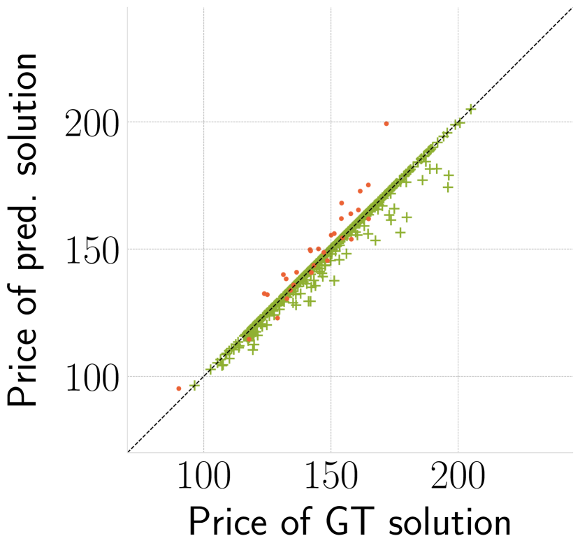
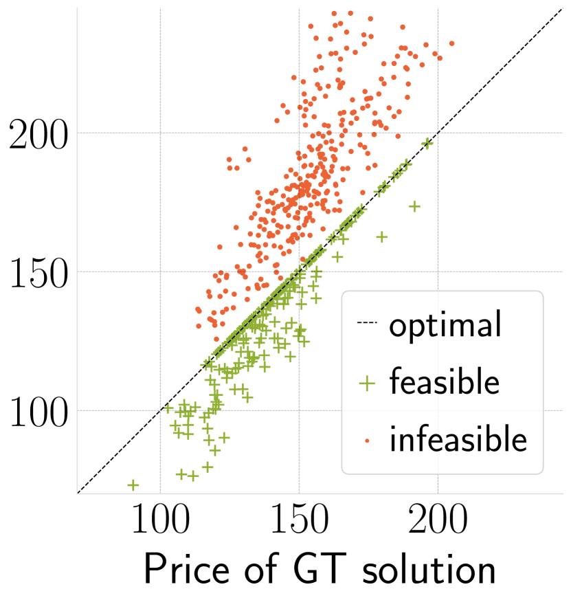
Additionally, we provide a qualitative analysis of the results on the Knapsack task. In Fig. 14 we compare the total ground-truth price of the predicted instances to the total price of the ground-truth solutions on a single evaluation of the trained models.

The plots show that CombOptNet is achieving much better results than CVXPY. The total prices of the predictions are very close to the optimal prices and only a few predictions are infeasible, while CVXPY tends to predict infeasible solutions and only a few predictions have objective values matching the optimum.

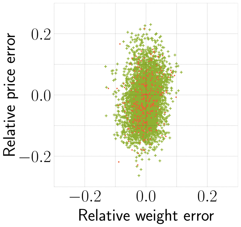
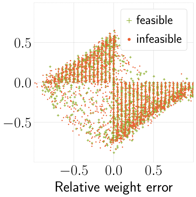
In Fig. 15 we compare relative errors on the individual item weights and prices on the same evaluation of the trained models as before. Since (I)LP costs are scale invariant, we normalize predicted price vector to match the size of the ground-truth price vector before the comparison.

CombOptNet shows relatively small normally distributed errors on both prices and weights, precisely as expected from the prediction of a standard network. CVXPY reports much larger relative errors on both prices and weights (note the different plot scale). The vertical lines correspond to the discrete steps of ground-truth item weights in the dataset. Unsurprisingly, the baseline usually tends to either overestimate the price and underestimate the item weight, or vice versa, due to similar effects of these errors on the predicted solution.

(a) CombOptNet

(b) CVXPY

Figure 14: Prices analysis for the Knapsack demonstration. For each test set instance, we plot the total price of the predicted solution over the total price of the ground-truth solution. Predicted solutions which total weight exceeds the knapsack capacity are colored in red (cross).

(a) CombOptNet

(b) CVXPY

Figure 15: Qualitative analysis of the errors on weights and prices in the Knapsack demonstration. We plot the relative error between predicted and ground-truth item prices over the relative error between predicted and ground-truth item weights. Colors denote whether the predicted solution is feasible in terms of ground-truth weights.

A.4 Ablations

We ablate the choices in our architecture and model design on the Random Constraints (RC) and Weighted Set Covering (WSC) tasks. In Tab. 8 and 9 we report constraint parametrization, choice of basis, and minima softening ablations.

The ablations show that our parametrization with learnable origins is consistently among the best ones. Without learnable origins, the performance is highly dependend on the origin of the coordinate system in which the directly learned parameters $({\bm{A}},{\bm{b}})$ are defined.

The choice of basis in the gradient decomposition shows a large impact on performance. Our basis $\Delta$ (9) is outperforming the canonical one in the binary RC and WSC demonstration, while showing performance similar to the canonical basis in the dense RC case. The canonical basis produces directions for the computation of ${\bm{y}}_{k}^{\prime}$ that in many cases point in very different directions than the incoming descent direction. As a result, the gradient computation leads to updates that are very detached from the original incoming gradient.

Finally, the softened minimum leads to increased performance in all demonstrations. This effect is apparent particularly in the case of a binary solution space, as the constraints can have a relevant impact on the predicted solution ${\bm{y}}$ over large distances. Therefore, only updating the constraint which is closest to the predicted solution ${\bm{y}}$, as it is the case for a hard minimum, gives no gradient to constraints that may potentially have had a huge influence on ${\bm{y}}$.

Appendix B Method

B.1 Fixed Constraints

In the paper we omitted the discussion of the effect of fixed (i.e. not learnable) constraints on the presented update rules. In our experiments, we assumed fixed feasible region to be a hypercube $[l,u]^{n}$ with $l,u\in{\mathbb{Z}},l<z$. Fixed constraints can cause problems, as our decomposition only guarantees that the targets ${\bm{y}}^{\prime}_{k}$ are integer points, but their feasibility w.r.t. to the fixed constraints is not guaranteed. Therefore, our assumption of ${\bm{y}}^{\prime}_{k}$ being an attainable target can be violated.

Table 8: Ablations of CombOptNet on Random Constraints demonstration. Reported is evaluation accuracy (${\bm{y}}={\bm{y}}^{*}$ in %) for $m=1,2,4,8$ ground-truth constraints. Statistics are over 20 restarts (2 for each of the 10 dataset seeds).

		Method	1	2	4	8
binary	param.	learnable origins	97.8  $\pm$  0.7	94.2  $\pm$  10.1	77.4  $\pm$  13.5	46.5  $\pm$  12.4
		direct (origin at corner)	97.4  $\pm$  1.0	94.9  $\pm$  7.0	59.0  $\pm$  26.8	26.9  $\pm$  10.3
		direct (origin at center)	98.0  $\pm$  0.5	97.1  $\pm$  0.6	70.5  $\pm$  19.1	44.6  $\pm$  5.9
	basis	$\Delta$ basis	97.8  $\pm$  0.7	94.2  $\pm$  10.1	77.4  $\pm$  13.5	46.5  $\pm$  12.4
		canonical	96.3  $\pm$  1.9	70.8  $\pm$  4.1	14.4  $\pm$  3.2	2.7  $\pm$  0.9
	min	hard		83.1  $\pm$  13.2	55.4  $\pm$  18.9	37.7  $\pm$  8.7
		soft ($\tau=0.5$)	97.8  $\pm$  0.7	94.2  $\pm$  10.1	77.4  $\pm$  13.5	46.5  $\pm$  12.4
		soft ($\tau=1.0$)		95.7  $\pm$  2.2	70.2  $\pm$  14.1	36.0  $\pm$  9.7
dense	param.	learnable origins	87.3  $\pm$  2.5	70.2  $\pm$  11.6	29.6  $\pm$  10.4	2.3  $\pm$  1.2
		direct (origin at corner)	86.7  $\pm$  3.0	74.6  $\pm$  3.6	32.6  $\pm$  13.7	2.8  $\pm$  0.5
		direct (origin at center)	83.0  $\pm$  6.1	43.8  $\pm$  13.2	11.6  $\pm$  3.1	1.1  $\pm$  0.5
	basis	$\Delta$ basis	87.3  $\pm$  2.5	70.2  $\pm$  11.6	29.6  $\pm$  10.4	2.3  $\pm$  1.2
		canonical	88.6  $\pm$  1.4	71.6  $\pm$  1.6	26.8  $\pm$  4.1	4.0  $\pm$  0.7
	min	hard		70.8  $\pm$  15.1	21.4  $\pm$  10.7	2.2  $\pm$  2.1
		soft ($\tau=0.5$)	89.1  $\pm$  2.8	70.2  $\pm$  11.6	29.6  $\pm$  10.4	2.3  $\pm$  1.2
		soft ($\tau=1.0$)		73.0  $\pm$  12.1	31.9  $\pm$  11.7	2.2  $\pm$  1.5

Table 9: Ablations of CombOptNet on Weighted Set Covering. Reported is evaluation accuracy (${\bm{y}}={\bm{y}}^{*}$ in %) for $m=4,6,8,10$ ground-truth constraints. Statistics are over 20 restarts (2 for each of the 10 dataset seeds).

	Method	4	6	8	10
param.	learnable origins	100  $\pm$  0.0	97.2  $\pm$  6.4	79.7  $\pm$  12.1	56.7  $\pm$  14.8
	direct (origin at corner)	99.4  $\pm$  2.9	94.1  $\pm$  16.4	78.5  $\pm$  15.7	47.7  $\pm$  17.9
	direct (fixed origin at 0)	99.9  $\pm$  0.6	87.6  $\pm$  6.4	65.3  $\pm$  11.9	46.7  $\pm$  11.5
basis	$\Delta$ basis	100  $\pm$  0.0	97.2  $\pm$  6.4	79.7  $\pm$  12.1	56.7  $\pm$  14.8
	canonical	8.4  $\pm$  13.3	2.0  $\pm$  2.6	0.2  $\pm$  0.3	0.0  $\pm$  0.1
min	hard	88.2  $\pm$  13.4	64.3  $\pm$  14.6	45.1  $\pm$  14.1	32.3  $\pm$  17.4
	soft ($\tau=0.5$)	100  $\pm$  0.0	97.2  $\pm$  6.4	79.7  $\pm$  12.1	56.7  $\pm$  14.8
	soft ($\tau=1.0$)	99.9  $\pm$  0.4	95.6  $\pm$  9.6	70.3  $\pm$  15.5	51.2  $\pm$  16.4
	soft ($\tau=2.0$)	98.8  $\pm$  3.1	90.6  $\pm$  14.3	66.4  $\pm$  12.5	51.2  $\pm$  9.5
	soft ($\tau=5.0$)	97.5  $\pm$  11.1	90.2  $\pm$  9.1	64.2  $\pm$  11.8	49.7  $\pm$  10.4

In our cases, we ensure the feasibility of the targets by first projecting ${\bm{y}}-\mathrm{d}{\bm{y}}$ into the hypercube as

$$({\bm{y}}^{\prime}_{\text{proj}})_{i}=\max(\min(y_{i}-\mathrm{d}y_{i},u),l)$$ (12)

and then decomposing the projected gradient

$$\mathrm{d}{\bm{y}}_{\text{proj}}={\bm{y}}-{\bm{y}}^{\prime}_{\text{proj}}$$ (13)

into integer steps as before.

B.2 Decomposition vs. Ground Truth

In the case of direct access to the ground-truth solution ${\bm{y}}^{*}$ (i.e. when CombOptNet is the last component in the architecture), we can always use ${\bm{y}}^{*}$ as a replacement for our targets ${\bm{y}}^{\prime}_{k}$, and there is no need to decompose the incoming gradient. In our demonstrations, we do in principle have access to ${\bm{y}}^{*}$, but, we still employ our decomposition to demonstrate the applicability of CombOptNet also in the general case.

B.3 Proofs

To recover the situation from the method section, set ${\bm{x}}$ as one of the inputs ${\bm{A}}$, ${\bm{b}}$, or ${\bm{c}}$.

Proposition 2.

Let ${\bm{y}}\colon\mathbb{R}^{\ell}\to\mathbb{R}^{n}$ be differentiable at ${\bm{x}}\in\mathbb{R}^{\ell}$ and let $L\colon\mathbb{R}^{n}\to\mathbb{R}$ be differentiable at ${\bm{y}}={\bm{y}}({\bm{x}})\in\mathbb{R}^{n}$. Denote $\mathrm{d}{\bm{y}}=\partial L/\partial{\bm{y}}$ at ${\bm{y}}$. Then the distance between ${\bm{y}}({\bm{x}})$ and ${\bm{y}}-\mathrm{d}{\bm{y}}$ is minimized along the direction $\partial L/\partial{\bm{x}}$, where $\partial L/\partial{\bm{x}}$ stands for the derivative of $L({\bm{y}}({\bm{x}}))$ at ${\bm{x}}$.

Proof.

For $\xi\in\mathbb{R}^{\ell}$, let $\varphi(\xi)$ denote the distance between ${\bm{y}}({\bm{x}}-\xi)$ and the target ${\bm{y}}({\bm{x}})-\mathrm{d}{\bm{y}}$, i.e.

$$\varphi(\xi)=\bigl{\|}{\bm{y}}({\bm{x}}-\xi)-{\bm{y}}({\bm{x}})+\mathrm{d}{\bm{y}}\bigr{\|}.$$

There is nothing to prove when $\mathrm{d}{\bm{y}}=0$ as ${\bm{y}}(x)={\bm{y}}-\mathrm{d}{\bm{y}}$ and there is no room for any improvement. Otherwise, $\varphi$ is positive and differentiable in a neighborhood of zero. The Fréchet derivative of $\varphi$ reads as

$$\varphi^{\prime}(\xi)=\frac{-\bigl{[}{\bm{y}}({\bm{x}}-\xi)-{\bm{y}}({\bm{x}})+\mathrm{d}{\bm{y}}\bigr{]}\cdot\frac{\partial{\bm{y}}}{\partial{\bm{x}}}({\bm{x}}-\xi)}{\bigl{\|}{\bm{y}}({\bm{x}}-\xi)-{\bm{y}}({\bm{x}})+\mathrm{d}{\bm{y}}\bigr{\|}},$$

hence

$$\varphi^{\prime}(0)=-\frac{1}{\|\mathrm{d}{\bm{y}}\|}\frac{\partial L}{\partial{\bm{y}}}\cdot\frac{\partial{\bm{y}}}{\partial{\bm{x}}}=-\frac{1}{\|\mathrm{d}{\bm{y}}\|}\frac{\partial L}{\partial{\bm{x}}},$$ (14)

where the last equality follows by the chain rule. Therefore, the direction of the steepest descent coincides with the direction of the derivative $\partial L/\partial{\bm{x}}$, as $\|\mathrm{d}{\bm{y}}\|$ is a scalar. ∎

Proof of Proposition 1.

We prove that

$$\sum_{j=\ell}^{n}u_{j}{\bm{e}}_{k_{j}}=\sum_{j=\ell}^{n}\lambda_{j}\Delta_{j}-|u_{\ell}|\sum_{j=1}^{\ell-1}\operatorname{sign}(u_{j}){\bm{e}}_{k_{j}}$$ (15)

for every $\ell=1,\ldots,n$, where we abbreviate $u_{j}=\mathrm{d}{\bm{y}}_{k_{j}}$. The claimed equality (3) then follows from (15) in the special case $\ell=1$.

We proceed by induction. In the first step we show (15) for $\ell=n$. Definition of $\Delta_{n}$ (9) yields

$$\lambda_{n}\Delta_{n}-|u_{n}|\sum_{j=1}^{n-1}\operatorname{sign}(u_{j}){\bm{e}}_{k_{j}}$$

$$\quad=|u_{n}|\sum_{j=1}^{n}\operatorname{sign}(u_{j}){\bm{e}}_{k_{j}}-|u_{n}|\sum_{j=1}^{n-1}\operatorname{sign}(u_{j}){\bm{e}}_{k_{j}}$$

$$\quad=u_{n}{\bm{e}}_{k_{n}}.$$

Now, assume that (15) holds for $\ell+1\geq 2$. We show that (15) holds for $\ell$ as well. Indeed,

$$\sum_{j=\ell}^{n}\lambda_{j}\Delta_{j}-|u_{\ell}|\sum_{j=1}^{\ell-1}\operatorname{sign}(u_{j}){\bm{e}}_{k_{j}}$$

$$\quad=\sum_{j=\ell+1}^{n}\lambda_{j}\Delta_{j}-|u_{\ell+1}|\sum_{j=1}^{\ell}\operatorname{sign}(u_{j}){\bm{e}}_{k_{j}}+\lambda_{\ell}\Delta_{\ell}$$

$$\qquad+|u_{\ell+1}|\sum_{j=1}^{\ell}\operatorname{sign}(u_{j}){\bm{e}}_{k_{j}}-|u_{\ell}|\sum_{j=1}^{\ell-1}\operatorname{sign}(u_{j}){\bm{e}}_{k_{j}}$$

$$\quad=\sum_{j={\ell+1}}^{n}u_{j}{\bm{e}}_{k_{j}}+\bigl{(}|u_{\ell}|-|u_{\ell+1}|\bigr{)}\sum_{j=1}^{\ell}\operatorname{sign}(u_{j}){\bm{e}}_{k_{j}}$$

$$\qquad+|u_{\ell+1}|\sum_{j=1}^{\ell}\operatorname{sign}(u_{j}){\bm{e}}_{k_{j}}-|u_{\ell}|\sum_{j=1}^{\ell-1}\operatorname{sign}(u_{j}){\bm{e}}_{k_{j}}$$

$$\quad=\sum_{j={\ell+1}}^{n}u_{j}{\bm{e}}_{k_{j}}+\operatorname{sign}(u_{\ell})|u_{\ell}|{\bm{e}}_{k_{\ell}}=\sum_{j=\ell}^{n}u_{j}{\bm{e}}_{k_{j}},$$

where we used the definitions of $\Delta_{\ell}$ and $\lambda_{\ell}$. ∎

References

- Agrawal et al. (2019a) Agrawal, A., Amos, B., Barratt, S., Boyd, S., Diamond, S., and Kolter, J. Z. Differentiable convex optimization layers. In Advances in Neural Information Processing Systems, pp. 9562–9574, 2019a.
- Agrawal et al. (2019b) Agrawal, A., Barratt, S., Boyd, S., Busseti, E., and Moursi, W. M. Differentiating through a cone program. J. Appl. Numer. Optim, 1(2):107–115, 2019b.
- Amos (2019) Amos, B. Differentiable optimization-based modeling for machine learning. PhD thesis, PhD thesis. Carnegie Mellon University, 2019.
- Amos & Kolter (2017) Amos, B. and Kolter, J. Z. Optnet: Differentiable optimization as a layer in neural networks. In International Conference on Machine Learning, pp. 136–145, 2017.
- Amos & Yarats (2020) Amos, B. and Yarats, D. The differentiable cross-entropy method. In International Conference on Machine Learning, pp. 291–302, 2020.
- Balcan et al. (2018) Balcan, M.-F., Dick, T., Sandholm, T., and Vitercik, E. Learning to branch. In International conference on machine learning, pp. 344–353, 2018.
- Balunovic et al. (2018) Balunovic, M., Bielik, P., and Vechev, M. Learning to solve SMT formulas. In Advances in Neural Information Processing Systems, pp. 10317–10328, 2018.
- Battaglia et al. (2018) Battaglia, P., Hamrick, J. B. C., Bapst, V., Sanchez, A., Zambaldi, V., Malinowski, M., Tacchetti, A., Raposo, D., Santoro, A., Faulkner, R., Gulcehre, C., Song, F., Ballard, A., Gilmer, J., Dahl, G. E., Vaswani, A., Allen, K., Nash, C., Langston, V. J., Dyer, C., Heess, N., Wierstra, D., Kohli, P., Botvinick, M., Vinyals, O., Li, Y., and Pascanu, R. Relational inductive biases, deep learning, and graph networks. arXiv:1806.01261, 2018.
- Bello et al. (2016) Bello, I., Pham, H., Le, Q. V., Norouzi, M., and Bengio, S. Neural combinatorial optimization with reinforcement learning. arXiv:1611.09940, 2016.
- Berthet et al. (2020) Berthet, Q., Blondel, M., Teboul, O., Cuturi, M., Vert, J.-P., and Bach, F. Learning with differentiable perturbed optimizers. In Advances in Neural Information Processing Systems, pp. 9508–9519, 2020.
- Bertinetto et al. (2019) Bertinetto, L., Henriques, J. F., Torr, P. H., and Vedaldi, A. Meta-learning with differentiable closed-form solvers. In International Conference on Learning Representations, 2019.
- Conneau et al. (2017) Conneau, A., Kiela, D., Schwenk, H., Barrault, L., and Bordes, A. Supervised learning of universal sentence representations from natural language inference data. In Conference on Empirical Methods in Natural Language Processing, pp. 670–680, Copenhagen, Denmark, 2017. Association for Computational Linguistics.
- Cplex (2009) Cplex, I. I. V12. 1: User’s Manual for CPLEX. International Business Machines Corporation, 46(53):157, 2009.
- Dalal et al. (2018) Dalal, G., Dvijotham, K., Vecerik, M., Hester, T., Paduraru, C., and Tassa, Y. Safe exploration in continuous action spaces. arXiv:1801.08757, 2018.
- Diamond & Boyd (2016) Diamond, S. and Boyd, S. CVXPY: A Python-embedded modeling language for convex optimization. Journal of Machine Learning Research, 17(83):1–5, 2016.
- Djolonga & Krause (2017) Djolonga, J. and Krause, A. Differentiable learning of submodular models. In Advances in Neural Information Processing Systems, pp. 1013–1023, 2017.
- Domke (2012) Domke, J. Generic methods for optimization-based modeling. In Artificial Intelligence and Statistics, pp. 318–326, 2012.
- Donti et al. (2017) Donti, P., Amos, B., and Kolter, J. Z. Task-based end-to-end model learning in stochastic optimization. In Advances in Neural Information Processing Systems, pp. 5484–5494, 2017.
- Elmachtoub & Grigas (2020) Elmachtoub, A. N. and Grigas, P. Smart “predict, then optimize”. arXiv:1710.08005, 2020.
- Ferber et al. (2020) Ferber, A., Wilder, B., Dilkina, B., and Tambe, M. MIPaaL: Mixed integer program as a layer. In AAAI Conference on Artificial Intelligence, volume 34, pp. 1504–1511, 2020.
- Fey et al. (2020) Fey, M., Lenssen, J. E., Morris, C., Masci, J., and Kriege, N. M. Deep graph matching consensus. In International Conference on Learning Representations, 2020.
- Gould et al. (2016) Gould, S., Fernando, B., Cherian, A., Anderson, P., Cruz, R. S., and Guo, E. On differentiating parameterized argmin and argmax problems with application to bi-level optimization. arXiv:1607.05447, 2016.
- Graves et al. (2014) Graves, A., Wayne, G., and Danihelka, I. Neural turing machines. arXiv:1410.5401, 2014.
- Graves et al. (2016) Graves, A., Wayne, G., Reynolds, M., Harley, T., Danihelka, I., Grabska-Barwińska, A., Colmenarejo, S. G., Grefenstette, E., Ramalho, T., Agapiou, J., Badia, A. P., Hermann, K. M., Zwols, Y., Ostrovski, G., Cain, A., King, H., Summerfield, C., Blunsom, P., Kavukcuoglu, K., and Hassabis, D. Hybrid computing using a neural network with dynamic external memory. Nature, 538(7626):471–476, October 2016.
- Gurobi Optimization (2019) Gurobi Optimization, L. Gurobi optimizer reference manual, 2019. URL http://www.gurobi.com.
- Khalil et al. (2017) Khalil, E., Dai, H., Zhang, Y., Dilkina, B., and Song, L. Learning combinatorial optimization algorithms over graphs. In Advances in Neural Information Processing Systems, pp. 6348–6358, 2017.
- Kingma & Ba (2014) Kingma, D. P. and Ba, J. Adam: A method for stochastic optimization. In International Conference on Learning Representations, 2014.
- Kool et al. (2018) Kool, W., van Hoof, H., and Welling, M. Attention, learn to solve routing problems! In International Conference on Learning Representations, 2018.
- Lee et al. (2019) Lee, K., Maji, S., Ravichandran, A., and Soatto, S. Meta-learning with differentiable convex optimization. In Conference on Computer Vision and Pattern Recognition, pp. 10657–10665, 2019.
- Ling et al. (2018) Ling, C. K., Fang, F., and Kolter, J. Z. What game are we playing? End-to-end learning in normal and extensive form games. In International Joint Conference on Artificial Intelligence, 2018.
- Min et al. (2019) Min, J., Lee, J., Ponce, J., and Cho, M. SPair-71k: A Large-scale Benchmark for Semantic Correspondence. arXiv:1908.10543, 2019.
- Nair et al. (2020) Nair, V., Bartunov, S., Gimeno, F., von Glehn, I., Lichocki, P., Lobov, I., O’Donoghue, B., Sonnerat, N., Tjandraatmadja, C., Wang, P., Addanki, R., Hapuarachchi, T., Keck, T., Keeling, J., Kohli, P., Ktena, I., Li, Y., Vinyals, O., and Zwols, Y. Solving mixed integer programs using neural networks. arXiv:2012.13349, 2020.
- Nazari et al. (2018) Nazari, M., Oroojlooy, A., Snyder, L., and Takác, M. Reinforcement learning for solving the vehicle routing problem. In Advances in Neural Information Processing Systems, pp. 9839–9849, 2018.
- Niculae et al. (2018) Niculae, V., Martins, A., Blondel, M., and Cardie, C. Sparsemap: Differentiable sparse structured inference. In International Conference on Machine Learning, pp. 3799–3808, 2018.
- Richardson (2001) Richardson, L. The knapsack problem, the game of premature optimization, 2001. URL https://www.crummy.com/software/if/knapsack/.
- Rolínek et al. (2020a) Rolínek, M., Musil, V., Paulus, A., Vlastelica, M., Michaelis, C., and Martius, G. Optimizing ranking-based metrics with blackbox differentiation. In Conference on Computer Vision and Pattern Recognition, 2020a.
- Rolínek et al. (2020b) Rolínek, M., Swoboda, P., Zietlow, D., Paulus, A., Musil, V., and Martius, G. Deep graph matching via blackbox differentiation of combinatorial solvers. In European Conference on Computer Vision, pp. 407–424, 2020b.
- Tan et al. (2020) Tan, Y., Terekhov, D., and Delong, A. Learning linear programs from optimal decisions. In Advances in Neural Information Processing Systems, pp. 19738–19749, 2020.
- Veličković et al. (2018) Veličković, P., Cucurull, G., Casanova, A., Romero, A., Lio, P., and Bengio, Y. Graph attention networks. In International Conference on Learning Representations, 2018.
- Veličković et al. (2020) Veličković, P., Ying, R., Padovano, M., Hadsell, R., and Blundell, C. Neural execution of graph algorithms. In International Conference on Learning Representations, 2020.
- Vlastelica et al. (2020a) Vlastelica, M., Paulus, A., Musil, V., Martius, G., and Rolínek, M. Differentiation of blackbox combinatorial solvers. In International Conference on Learning Representations, 2020a.
- Vlastelica et al. (2020b) Vlastelica, M., Rolinek, M., and Martius, G. Discrete planning with end-to-end trained neuro-algorithmic policies. ICML 2020, Graph Representation Learning Workshop, 2020b.
- Wallace et al. (2019) Wallace, E., Wang, Y., Li, S., Singh, S., and Gardner, M. Do NLP models know numbers? Probing numeracy in embeddings. In Conference on Empirical Methods in Natural Language Processing and the 9th International Joint Conference on Natural Language Processing, pp. 5310–5318, 2019.
- Wang et al. (2019) Wang, P.-W., Donti, P., Wilder, B., and Kolter, Z. SATNet: Bridging deep learning and logical reasoning using a differentiable satisfiability solver. In International Conference on Machine Learning, pp. 6545–6554, 2019.
- Wilder et al. (2019) Wilder, B., Ewing, E., Dilkina, B., and Tambe, M. End to end learning and optimization on graphs. In Advances in Neural Information Processing Systems, pp. 4672–4683, 2019.
- Zanfir & Sminchisescu (2018) Zanfir, A. and Sminchisescu, C. Deep learning of graph matching. In Conference on Computer Vision and Pattern Recognition, pp. 2684–2693, 2018.
- Zhang & Dietterich (2000) Zhang, W. and Dietterich, T. G. Solving combinatorial optimization tasks by reinforcement learning: A general methodology applied to resource-constrained scheduling. Journal of Artificial Intelligence Reseach, 1:1–38, 2000.