Reconstructing shared dynamics with a deep neural network
Abstract
Determining hidden shared patterns behind dynamic phenomena can be a gamechanger in multiple areas of research. Here we present the principles and show a method to identify hidden shared dynamics from time series by a two-module, feedforward neural network architecture: the Mapper-Coach network. We reconstruct unobserved, continuous latent variable input, the time series generated by a chaotic logistic map, from the observed values of two simultaneously forced chaotic logistic maps. The network has been trained to predict one of the observed time series based on its own past and conditioned on the other observed time series by error-back propagation. It was shown, that after this prediction have been learned successfully, the activity of the bottleneck neuron, connecting the mapper and the coach module, correlated strongly with the latent shared input variable. The method has the potential to reveal hidden components of dynamical systems, where experimental intervention is not possible.
pacs:
05.45.Tp, 05.45.-a, 05.45.Xt, 07.05.Kf, 07.05.MhI Introduction & Background
Theory of nonlinear dynamical systems has plenty to offer for neural architecture design. Here we take a dualistic approach, incorporating the principles of nonlinear time series techniques and the application of simple feedforward learning algorithms to achieve the reconstruction an unobserved common input of two observed chaotic dynamical systems.
A dynamical system has a state and an update rule. It can have a discrete time dynamics or it can be a continuous time flow. In the former, the state () is updated according to the update rule () thus gives rise to the future states of the system, which we observe through an observation function (, Eq. 1).
| (1) |
Where the , is a smooth (not necessarily invertible) mapping, is a smooth observation function which produces the time series ( ).
If we have no acces to the full system state but have an observation function like producing a time series (), we can still reconstruct the state up to a continuous transformation. Takens theoremTakens (1981) ensures that this topological equivalence has high probability, and shows that time delay embedding – shown in (2) – is such a reconstruction procedure.
| (2) |
Where is the reconstructed state at time .
In the case of directionally coupled systems, one can reconstruct the state of the driver from the state of the forced subsystem Stark (1999); Stark et al. (2003); Sugihara et al. (2012). Directed causal link leaves the fingerprint of the driver on the driven system such that the full coupled system’s state can be reconstructed or decoded from the observations of the driven system.
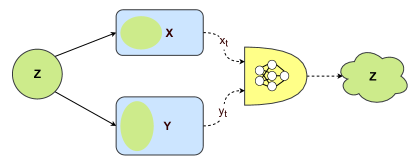
When a hidden process drives two subsystems, both subsystems contain a fingerprint of the latent variable that is encoded in their dynamics (Fig. 1). This redundancy can be leveraged to identify the existence hidden common drivers between subsystems Hirata and Aihara (2010); Benkő et al. (2018). Hirata et al. applied the technique of recurrence maps to identify the existence of the hidden common cause. Benko et al. measured the intrinsic dimensionality of reconstructed statespaces, thus identified the existence of the hidden common cause by determining the number of the redundant degrees of freedom (the mutual dimension Sugiyama and Borgwardt (2013)) between the reconstructed dynamics of the subsystems.
Since the redundant information about the shared hidden dynamics or common cause is present in the reconstructed states of the forced subsystems, then the question arises whether this information can be extracted from the time series or it is practically unidentifiable. In this article we show that not only the existence, but values of the shared dynamics can be reconstructed (up to a continuous transformation) by a new specific neural network architecture.
II Previous work
There are only a few methods to reconstruct hidden common input from multivariate time series observations and the use of these is restricted to specific types of hidden common inputs Sauer (2004); Wiskott and Sejnowski (2002).
Sauer demonstrated that reconstruction of common input from time series is possible by the Shared Dynamics Algorithm (SDA) if the observed dynamics is simpleSauer (2004, 2010). SDA builds on the shared dynamics reconstruction theorem, and makes possible to reconstuct unobserved and shared driver dynamics from time series observations of driven systems[1].
The steps of this family of algorithms are as follows:
-
1.
Time delay embedding of the time series with the shared dynamics, . The embedding dimension is resulting in reconstructed points .
-
2.
Pick the first variable () as reference for the equivalence classes. Choose neighborhoods from at times , and pick radius neighborhoods around. Map back the points within the neighborhoods onto , and connect the sets which are closer than in . Cluster the sets and choose representative points from the clusters.
In the end, the algorithm splits the points into equivalence classes, each class stands for a discretized value of the latent driver.
Wiskott and Sejnowski introduced Slow Feature Analysis (SFA) as a Blind Source Separation (BSS) technique Wiskott and Sejnowski (2002). The objective of BSS is to identify the true signal sources () from multivariate time series measurements (), which contain the source signals in a mixed way:
| (3) |
where is the time series, is the latent signal, -s are the source factors, is the invertible mixing function and the pair is a Latent Variable Model. The BSS problem is underdetermined in general, so additional assumptions on the data and the mixing function is required to find a unique solution. Such an assumption is that the sources were independent and non-gaussian like in linear Independent Component Analysis (ICA). It is also possible to identify independent features in the case of nonlinear mixing functions with Variational Auto-EncodersKhemakhem et al. (2019) and normalizing Flow-Based MethodsSorrenson, Rother, and Köthe (2020).
Slow Feature Analysis (SFA) solves the blind source separation problem for time seriesWiskott and Sejnowski (2002). It assumes that the latent signals are independent and temporally consistent, slowly changing:
| (4) |
The suitable mapping chosen by applying a filterbank on the original signal then performing PCA on whitened features to get slow features. This basic SFA method was implemeted recently using neural networks resulting in the slow flow modelPineau et al. (2020).
Wiskott showed that one can reconstruct slow hidden common dynamics from time series with SFAWiskott (2003).
However, no method existed yet, which can reconstruct a continuous hidden common input with fast dynamics. Here we introduce such a method in order to reconstruct fast and continuous latent shared dynamics from time series.
III Example: coupled logistic map system
We demonstrate the nonlinear state space reconstruction and the inference procedure for the latent process on coupled logistic map systems. The logistic map is a discrete time dynamical system exhibiting chaotic behaviour in a properly selected range of the parameter May (1976).
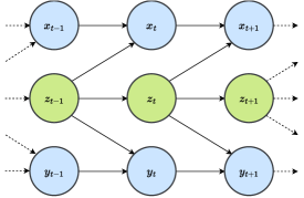
Let’s take three logistic maps coupled in a fork structure such that one drove the other two (Fig. 2, Eq. 5).
| (5) |
Where is a positive parameter and are coupling constants.
Let’s focus on the - subsystem, where unidirectionally drives . The state of the subsystem is the vector and the dynamics of the system can be written in the corresponding vector form:
| (6) |
where and are the state variables, is the parameter of the logistic map and are the coupling parameters. Furthermore, is a linear observation function such that . So values are observed from the system state, but the values remain hidden.
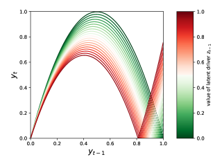
In the followings, we show can be reconstructed from one of the observed time series. We know from the theory Stark (1999) that we can reconstruct the state of the subsystem based on the observed variable time delay embedding:
| (7) |
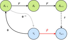
where is the scalar value of at time , and is the reconstructed state of the system almost everywhere . Here we neglect the ambiguity caused by the reflective boundary conditions needed to constrain the coupled dynamics in the square. This ambiguity can be ruled out by higher dimensional embeddings for example in dimensions the space would be an embedding of the -dimensional statespace Takens (1981). To see that truly described the state of the system almost everywhere, we show the mapping from to and build the dynamics in the reconstructed state space (Fig. 3).
First, we reorder the equation that realizes the mapping (Eq. (6)) to get the expression for and :
| (8) |
thus we have a mapping from to .
Also, we can write the the inverse of as:
| (9) |
By this, we demonstrated that there exists a one-to-one mapping between and , thus is a reconstructed state of the subsystem. We can define the dynamics on this reconstructed space, to predict future states (Fig. 3).
| (10) |
Let’s zoom out from the subsystem and see the full system, where is unobserved. To predict the value of , one needs the previous value of and according to the update rule in Eq. (5). Since contains all required information about , we can use in place of , and predict given , if the required mappings - , and - are also given. When these functions are unkown, one has to approximate them from data. For the function approximation, it is practical to use feedforward neural networks.
IV Results
IV.1 The proposed architecture: the Mapper-Coach network
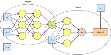
We reconstruct the hidden common input from a dataset generated by the logistic map system in Eq. (5). To extract the hidden driver, we set up a prediction task and a neural network architecture for function approximation (Fig. 5). We predict the value of based on as input. We split this task into two parts: first we estimate from and second we approximate the dynamics from the estimated state.
To estimate the hidden input we had to approximate the mapping (Eq.(8)), we implemented this function by a feedforward neural network: the Mapper module (Fig. 5). The input space is the reconstructed state space of and the output is the value of . But how to find the exact mapping from to , when is unobserved?
We use values from the other observed time series to guide the search for a good mapping. We attached a coach module (coach) to the output of the mapper and also channeled as additional direct input (Fig. 5). The output of the coach is a prediction on the current value of , therefore the subnetwork intends to implement the dynamics of from Eq. (5).
The fusion of the two parts is the Mapper-Coach network, which reconstructs the shared dynamics by the activity of hidden units at the meeting point of the two modules.
IV.2 Performance on the logistic map system
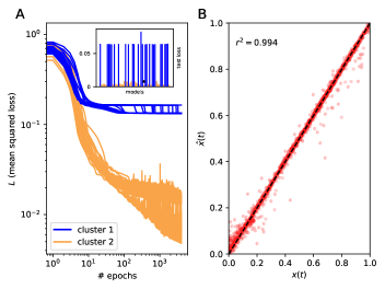
We trained the mapper-coach network with the backpropagation algorithm to predict at the output of the coach module, and found that the output of the mapper network reconstructed the hidden variable.
Prediction performance: The network produced very accurate predictions on after the learning procedure (, Fig. 6). We split the data into training, test and validation sets (, , , respectively), trained the network and evaluated the results on the latter sets. We reinitialized the training times with random weights, and selected the best-performing model for evaluation. According to the learning characteristics, we identified two clusters of the models (6 A). Half of the models were stuck in local minima (cluster 1, 25/50) and in half of the cases the learning was successful (cluster 2, 25/50).
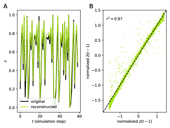
Reconstruction performance: We found that the mapper part of the network reconstructed the past values of the hidden common input() quiet accurately: the squared correlation between the mapper output () and the actual hidden common input was , (Fig 7). We detached the coach and investigated the output of the mapper by providing test inputs. The output reflected the values of , so the mapper network approximately implemented the mapping in Eq. (8).
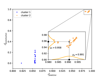
We showed that the prediction- and the reconstruction performance were related: the better the model predicted the better it reconstructed (Fig. 8). The trained network instances achieved different prediction performance on the test set, of the networks had high quality output. We plotted the prediction performance against the reconstruction performance for each model. We saw that better quality predictions implied better quality reconstructions (Fig. 8).
V Discussion
We demonstrated that reconstruction of a latent variable with fast and continuous state-space dynamics is possible with the backpropagation algorithm, but there are several challenges remain to be assessed.
SDA and SFA can reconstruct common drivers, but the usecases are restricted. In principle the SDA could be applied on elaborate systems, when the driver and observed dynamics is not discrete or one-dimensional and even for chaotic driver, but in practice it was only demonstrated to work on very simple discrete and one-dimensional examples. SFA can reconstruct the common latent input, but only if the its dynamics is slow. In contrast, the mapper-coach approach could reconstruct fast continuous variables.
We reconstructed the latent common input from example time series, leveraging the theoretical properties of the underlying coupled chaotic dynamical systems. We implemented the method by the Mapper-Coach network, where the mapper part realized the mapping and the coach implemented the one-step prediction-map .
The architecture of the network is asymmetric: the role of the and input is not equivalent. The reconstructed space of contains all information about the hidden variable , but the value lacks this information. The vital point is that the coach sips out the required information about from the input through the Mapper, and this information is only fully available in the , not in the input pathway.
To ensure that the mapper outputs information about the hidden variable, the dimensionality of the coach-input has to be minimal. In more complex systems, it could be more difficult to obtain this minimality. One possibility is that the number of output units from the mapper should equal to dimensionality of the common hidden dynamics. Also, the number of direct input units (from in the example) has to equal to the remaining degrees of freedom in which is independent from . Therefore, in this case, to determine the proper number of units for mapper output and -input, one has to investigate the intrinsic dimensionality and the mutual dimension between the embedded , variablesBenkő et al. (2020); Romano et al. (2016); Benkő et al. (2018). An other possibility would be to use sparse activity-regularization and cross-validation to restrict the information-capacity of the representational layer resulting in a bottleneck.
We demonstrated, that the proposed architecture works for a discrete time, deterministic (noise-free) dynamical system, but whether this approach is applicable to continuous flows and how robust it is to noise is yet to be investigated. Theoretically there are no obstacles for the former and – since state-space reconstruction can be robust up to moderate noise levelsCasdagli et al. (1991) – the latter can be handled in the case of low noise, or after noise-filtering.
This architecture gives a simple example on how to extract the information about the common latent variable, but other symmetric, autoencoder-based architectures are also applicable and can be the subject of further investigations.
Also, a possible research-path is the slow-flow realization of shared dynamics reconstruction which is yet to be implemented and tested.
We took a dynamical systems aspect through the paper, but there are connections to autoencoders, representation learning and hidden Markov modelsKingma and Welling (2014); Marino, Yue, and Mandt (2018). For example the reconstruction of the common dynamics by the proposed architecture can be seen as amortized inference in a conditional latent variable model. The coach part, which performs the prediction is the latent variable model conditioned on the value and the mapper part realizes the fast inference. Besides the fact that common latent inputs can be reconstructed, it is relevant to inspect that how the learned latent representations can be interpreted and used for prediction, compression, classification, anomaly detection, etc. Jakovac, Berenyi, and Posfay (2020); Jakovac (2021); Jakovac, Kurbucz, and Posfay (2022); Kurbucz, Pósfay, and Jakovác (2022).
VI Methods
VI.1 Data generation and handling
We generated data points according to Eq. (5) (, ) with reflective boundary condition on the interval. We embedded the variable, thus produced , and aligned the time-scale of and time series according to the time-shift produced by the embedding procedure. We splitted the data into training(80%), test (10%) and validation (10%) sets.
VI.2 Model implementation
VI.3 Training and evaluation
We randomly initialized the weights and started training with the batch size of and for epochs. We used the ADAM optimizer and mean squared loss function with default parameters except the learning rate (). We initialized instances of the network and selected the best performing model on the test set for further evaluation.
We used the coefficient of determination () to evaluate model test and validation performance. This metric is simply is the square of the Pearson correlation coefficient ():
| (11) |
where and are the sample points, are the sample means and the -s are the sample standard deviations. This coefficient describes the linear dependence between the two variables.
We computed between and the predicted values on the test set (Fig. 6). We have chosen the model with the best performance to see the hidden activations on the validation set.
We also calculated the between the ”true” hidden variable and the the output of the mapper network () on the validation set. We displayed these results on a time series plot an on a correlogram (Fig. 7).
We also computed the reconstructed values and the values for the not optimal models, and plotted the prediction performance against the reconstruction performance of the models (Fig. 8).
Data and Code availability
The data set and all the code can be found at https://github.com/phrenico/maco_commondriver.
Acknowledgments
The authors thank András Telcs and Marcell Stippinger for the valuable discussions on this topic.
References
- Takens (1981) F. Takens, “Detecting strange attractors in turbulence,” Dynamical Systems and Turbulence, Warwick 1980 898, 366–381 (1981), arXiv:arXiv:1011.1669v3 .
- Stark (1999) J. Stark, “Delay embeddings for foreced systems. I. Deterministic forcing,” Journal of Nonlinear Science 9, 255–332 (1999).
- Stark et al. (2003) J. Stark, D. S. Broomhead, M. E. Davies, and J. Huke, “Delay embeddings for forced systems. II. stochastic forcing,” Journal of Nonlinear Science 13, 519–577 (2003).
- Sugihara et al. (2012) G. Sugihara, R. May, H. Ye, C.-h. Hsieh, E. Deyle, M. Fogarty, and S. Munch, “Detecting Causality in Complex Ecosystems,” Science 338, 496–500 (2012).
- Hirata and Aihara (2010) Y. Hirata and K. Aihara, “Identifying hidden common causes from bivariate time series: A method using recurrence plots,” Physical Review E 81, 016203 (2010).
- Benkő et al. (2018) Z. Benkő, Á. Zlatniczki, M. Stippinger, D. Fabó, A. Sólyom, L. Erőss, A. Telcs, and Z. Somogyvári, “Complete Inference of Causal Relations between Dynamical Systems,” , 1–44 (2018), arXiv:1808.10806 .
- Sugiyama and Borgwardt (2013) M. Sugiyama and K. M. Borgwardt, “Measuring statistical dependence via the mutual information dimension,” IJCAI International Joint Conference on Artificial Intelligence , 1692–1698 (2013).
- Sauer (2004) T. D. Sauer, “Reconstruction of Shared nonlinear dynamics in a network,” Physical Review Letters 93, 1–4 (2004).
- Wiskott and Sejnowski (2002) L. Wiskott and T. J. Sejnowski, “Slow feature analysis: Unsupervised learning of invariances,” Neural Computation 14, 715–770 (2002).
- Sauer (2010) T. Sauer, “Detection of periodic driving in nonautonomous difference equations,” in Lecture Notes in Mathematics, Vol. 2002 (2010) pp. 301–309.
- Khemakhem et al. (2019) I. Khemakhem, D. P. Kingma, R. P. Monti, and A. Hyvärinen, “Variational Autoencoders and Nonlinear ICA: A Unifying Framework,” 108 (2019), arXiv:1907.04809 .
- Sorrenson, Rother, and Köthe (2020) P. Sorrenson, C. Rother, and U. Köthe, “Disentanglement by Nonlinear ICA with General Incompressible-flow Networks (GIN),” , 1–23 (2020), arXiv:2001.04872 .
- Pineau et al. (2020) E. Pineau, S. Razakarivony, T. Bonald, E. Pineau, S. Razakarivony, T. Bonald, T. Series, and S. Separation, “Time Series Source Separation with Slow Flows,” (2020).
- Wiskott (2003) L. Wiskott, “Estimating Driving Forces of Nonstationary Time Series with Slow Feature Analysis,” , 1–8 (2003), arXiv:0312317 [cond-mat] .
- May (1976) R. M. May, “Simple mathematical models with very complicated dynamics,” Nature 261, 459–467 (1976).
- Benkő et al. (2020) Z. Benkő, M. Stippinger, R. Rehus, A. Bencze, D. Fabó, B. Hajnal, L. Erőss, A. Telcs, and Z. Somogyvári, “Manifold-adaptive dimension estimation revisited,” , 1–21 (2020), arXiv:2008.03221 .
- Romano et al. (2016) S. Romano, O. Chelly, V. Nguyen, J. Bailey, and M. E. Houle, “Measuring dependency via intrinsic dimensionality,” in 2016 23rd International Conference on Pattern Recognition (ICPR), 4 (IEEE, 2016) pp. 1207–1212.
- Casdagli et al. (1991) M. Casdagli, S. Eubank, J. Farmer, and J. Gibson, “State space reconstruction in the presence of noise,” Physica D: Nonlinear Phenomena 51, 52–98 (1991).
- Kingma and Welling (2014) D. P. Kingma and M. Welling, “Auto-encoding variational bayes,” 2nd International Conference on Learning Representations, ICLR 2014 - Conference Track Proceedings , 1–14 (2014), arXiv:1312.6114 .
- Marino, Yue, and Mandt (2018) J. Marino, Y. Yue, and S. Mandt, “Iterative amortized inference,” 35th International Conference on Machine Learning, ICML 2018 8, 5444–5462 (2018), arXiv:1807.09356 .
- Jakovac, Berenyi, and Posfay (2020) A. Jakovac, D. Berenyi, and P. Posfay, “Understanding understanding: a renormalization group inspired model of (artificial) intelligence,” arXiv , 1–15 (2020), arXiv:2010.13482 .
- Jakovac (2021) A. Jakovac, “Time series analysis with dynamic law exploration,” (2021).
- Jakovac, Kurbucz, and Posfay (2022) A. Jakovac, M. T. Kurbucz, and P. Posfay, “Reconstruction of observed mechanical motions with artificial intelligence tools,” (2022).
- Kurbucz, Pósfay, and Jakovác (2022) M. T. Kurbucz, P. Pósfay, and A. Jakovác, “Linear laws of markov chains with an application for anomaly detection in bitcoin prices,” (2022).
- Van Rossum and Drake (2009) G. Van Rossum and F. L. Drake, Python 3 Reference Manual (CreateSpace, Scotts Valley, CA, 2009).
- Paszke et al. (2017) A. Paszke, S. Gross, S. Chintala, G. Chanan, E. Yang, Z. DeVito, Z. Lin, A. Desmaison, L. Antiga, and A. Lerer, “Automatic differentiation in pytorch,” (2017).