Primary and Secondary Social Media
Source Identification

Abstract

Social networks like Facebook and WhatsApp have enabled users to share images with other users around the world. Along with this has come the rapid spread of misinformation. One step towards verifying the authenticity of an image is understanding its origin, including it distribution history through social media. In this paper, we present a method for tracing the posting history of an image across different social networks. To do this, we propose a two-stage deep-learning-based approach, which takes advantage of cascaded fingerprints in images left by social networks during uploading. Our proposed system is not reliant upon metadata or similar easily falsifiable information. Through a series of experiments, we show that we are able to outperform existing social media source identification algorithms. and identify chains of social networks up to length two with over over 84% accuracy.

I Introduction

The widespread use of social media has resulted in the rapid spread of information, and with it, misinformation. As a result, a variety of multimedia forensic techniques have been developed to authenticate images and videos [1, 2, 3, 4, 5]. When determining the credibility of an image, it is often helpful to consider the credibility of the source. Prior forensics research aimed at determining an image’s source has largely fallen into two categories: camera model identification [6, 7, 8, 9, 10, 11, 12] and device identification [13, 14, 15, 16, 17, 18, 19]. Several of these techniques have been adapted to operate on video as well [1, 20, 21, 22, 23].

One important aspect of image source identification that has received comparably little attention is determining an image’s distribution channel; specifically determining which, if any, social network have been used to share an image. The posting history of images is of particular concern in the case of misinformation campaigns, which are typically launched over social media. In such campaigns, it is common for an image to be posted along with text which provides false context, such as claims of violent rioters at a peaceful protest. In such cases, knowing that the picture has been reposted, and does not belong to the purported author, can disprove the falsely supplied context.

When images are uploaded to a social media network, the hosting platform will often apply a series of processing operations to the image. The specific operations are proprietary, and therefore unknown, but include JPEG re-compression and re-sampling(i.e. resizing) as methods for reducing the size of the image to be stored by the platform. Processing operations such as these have been known to leave unique fingerprints; when operations are cascaded, fingerprints are likewise cascaded [24, 25, 26]. However when fingerprints are cascaded, older fingerprints are degraded or obscured. This means that reposting an image to a second social media platform can obscure the traces left by the original platform. Unless accounted for, this will result in decreased accuracy when determining a reposted image’s original network.

To date, comparatively little work has been done toward identifying an image’s posting history. Amerini et al. used traces of double JPEG compression to identify which social media site an image was posted to [27]. This technique, however, is only designed to operate on images posted to a single social network. The authors refined this by developing a CNN-based approach capable of operating on images that may have been uploaded to multiple networks [28]. This system, however, can only identify the last social network an image is posted to. Recently, Phan et al. introduced a system to identify re-posted images, and the social networks they were reposted from [29]. To do this, the authors used multi-JPEG compression traces, as well as image-wide features like quantization table coefficients, image dimensions, and lossless coding parameters.

While prior work provides important first steps toward robust social media source identification, it still has several shortcomings. The reliance on easily mutable features such as image dimensions and the ordering of coding tables makes Phan et al.’s system unreliable when presented with unseen image sizes and lossless reordering of the JPEG image file.

These features can easily be altered, even unintentionally, and without these features, the system’s accuracy is reduced by as much as 30%. Therefore, when attempting to determine the posting history of an image, we must rely on intrinsic or embedded features, as opposed to those easily altered features such as file structure. Furthermore, if these intrinsic features could be identified from several smaller regions of an image, a system could be developed to identify inconsistencies within the image, offering information as to its authenticity.

In light of this we would like to design a system that can accurately determine the posting history of an image patch, that is not reliant on unreliable features. Future adaptation of this system could then localize inconsistencies in the posting history within an image.

In this paper, we propose a patch-based system for tracing the social network posting history of an image. Unlike the current state of the art, our system does not rely on falsifiable metadata or non-local features such as image dimensions. We will show that our system is able to outperform existing techniques that do not make use of these features.

II System Architecture

To perform social media source identification, we propose a system which leverages both deep learning techniques and traditional forensic fingerprints. Our proposed system comprises two stages. The first stage determines the social media network which most recently hosted an image. This is leveraged in the second stage to determine the previous host network, if any.

This two-stage architecture offers benefits over using a single classifier. It has been shown that the traces left by one editing operation can be obscured or overwritten by another editing operation [24, 25, 26, 30]. The way in which the original traces are obscured is dependent on the editing operation. By using a two-stage system, and first identifying the latest social network, we can use more specialized classifiers to discriminate between the potential previous networks.

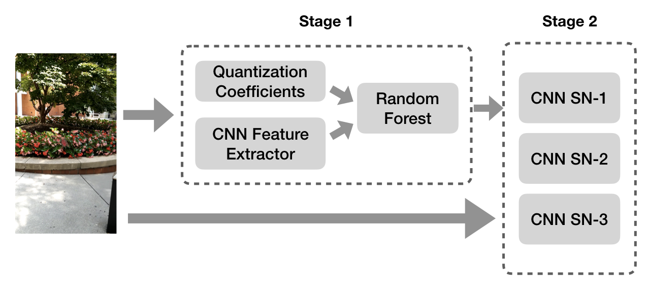
Figure 1: Proposed system architecture. The output of Stage 1 is used to determine the appropriate Stage 2 classifier.

II-A Stage 1

The first stage of our system determines the social media platform that most recently hosted an image. This stage uses the deep features of a CNN trained to discriminate between social networks, as features for classification. These deep features, as well as compression parameters of the image, are fed to a random forest classifier. On the basis of these features, the classifier is able to make highly accurate decisions.

In order to learn discriminating features, we first train a CNN to classify images based on their social media of origin. We then remove the decision function of the network, and use the output neuron activations as a feature vector. We use a CNN architecture comprising a single convolutional layer, followed by four convolutional blocks (Convolution, batch normalization, tanh activation and max pooling), then two full-connected blocks (matrix multiplication, activation), and an output layer where each neuron corresponds to a single class. The first convolutional layer contains 6 filters, each of size $3\times 3$. The four convolutional blocks have 96 $7\times 7$ filters, then 64 $5\times 5$ filters, 64 $5\times 5$ filters, and finally 128 filters of size $1\times 1$. The full-connected layers each have 200 neurons [31]. Instead of designating one output neuron for each social media processing chain, we assign one neuron for each social media platform. For example, the Google Photos class encompasses all images which have been uploaded to Facebook or WhatsApp before being posted to Google Photos, as well as images which were only posted to Google Photos.

Because errors made in the first stage will propagate through to following stage system, it is critical that the classifier used in this stage is as accurate as possible. In order to increase the accuracy of our first stage, we supplement the features learned by the CNN with features extracted from the image’s encoding process. We observed that all images remained JPEG-compressed when downloaded from a social network. However the parameters of this compression, specifically the quantization table corresponding to the luma channel, were often changed.

To leverage this change, we extract the first 9 AC coefficients of the luma-channel quantization table stored in the image. These features have been shown to be useful for other forensic tasks [32]. We use these coefficients, and the activations of our CNN, as the basis for classification. For an image patch $X$, our Stage 1 classification, $C$, is given by,

$$C=\mathcal{F}(\text{CNN(X)}||\mathcal{Q}(X)),$$ (1)

Where $\text{CNN}(X)$ is the deep features obtained by the CNN, $\mathcal{Q}(X)$ indicates the quantization table coefficients of the image, and $||$ is the concatenation of the two vectors. $\mathcal{F}$ is the random forest classifier.

Intuitively, our Stage 1 classification is attained by first concatenating the output neuron activations of the CNN with the selected quantization table coefficients. This feature vector is then fed to a random forest classifier, which is able to achieve a higher accuracy than the CNN alone.

II-B Stage 2

The second stage of our system determines the previous social media network of an image, given an image and that image’s latest social network. This stage contains one classifier for each social network class in the first stage. For the classifiers in this stage, we use the same CNN architecture as the feature extractor in the first stage.

Each classifier in this stage is predicated on the input image’s latest social media network and attempts to discern the images previous social network. To do this, we train each classifier only on images which share a latest social media network, and designate one output neuron for each candidate previous social media network. For example, one classifier will take as input, an image which Stage 1 identified as Google Photos, and will have output neurons corresponding to None, Facebook(HQ), Facebook(LQ), and WhatsApp. If the maximum activation of this CNN corresponds to Facebook(HQ), then the image is classified as having been uploaded to Facebook(HQ), then downloaded and posted to Google Photos.

This same structure is replicated for every other social network. Therefore, for any social media source identifiable by the first stage of our system, there is a corresponding second-stage classifier to determine the previous social network to host the image in question. Figure 1 illustrates the whole system architecture. As we will show,this system outperforms the current state of the art system which considers each possible permutation of social networks concurrently.

III Experimental Results

III-A Dataset

To experimentally verify our system, we created a dataset of images with 11 unique social media upload chains, with a maximum of two social networks in a chain. In order to create this dataset, we used a subset of images from the VISION [33] dataset. The VISION dataset contains natural(NAT) images, as well as copies of those images uploaded to each of Facebook with the high quality setting (FBH), Facebook with the low-quality setting (FBL), and WhatsApp (WA). For our dataset, we took 1219 natural images, and all social media edited copies from five different camera models of the VISION database. We uploaded additional copies of the natural images to Google Photos (GOG). This resulted in four social network processing chains of length one (natural images uploaded to Facebook-HQ, Facebook-LQ, WhatsApp, or Google Photos), and one chain of length zero (natural images).

Next, three processing chains of length two were created by reposting all images with a processing chain of length one to Google Photos, excluding those which had already been posted to Google Photos. Three more chains of length two were created by reposting images with a processing chain of length one to Facebook-HQ, except for those which had already been posted to Facebook-HQ. Due to resource and time constraints, the other length-two processing chains could not be investigated. This resulted in nearly 13,500 images from 11 unique social media processing chains.

Images were given both a primary and a secondary label. The primary label, an upper-case code from {NAT, FBH, FBL, WA, GOG} corresponds to the last social media that an image was uploaded to, which the first stage of our system is built to identify. An image’s secondary label, a lower-case code from one of {nat, fbh, fbl, wa, gog} corresponds to the social media platform that an image was uploaded to before the latest one. For example, an image with the label “fblGOG” was first uploaded to Facebook-LQ, then uploaded to Google Photos. An image labeled “natGOG” was only uploaded to Google Photos and no other platforms.

III-B Stage 1

To train our Stage 1 classifier, we first trained our feature extraction CNN. Our dataset was divided into training and testing images by randomly selecting 10% of the images from each class for testing, and leaving the rest for training. From the training images, we extracted 960,000 image patches of size $64\times 64$ from images with each of the five primary labels. From the testing images, 96,000 patches were extracted for each class. We then trained our CNN feature extractor using stochastic gradient descent with an initial learning rate of $0.001$, that was halved every 3 epochs for 50 epochs. We also extracted 240,000 training patches and 24,000 testing patches of size $128\times 128$, as well as 60,000 training and 6,000 testing patches of size $256\times 256$. These datasets were used to train two additional feature extractors using the same training procedure.

TABLE I: Accuracy of classifiers trained to identify patch’s latest social media network.

Patch Size	64	128	256
Amerini et al. [28]	78.1%	87.7%	91.7%
Proposed CNN	83.53%	92.67%	86.41%
Proposed Stage 1	93.92%	94.50%	94.75%

After each CNN was trained, we concatenated the output activations of each training patch with the first 9 AC quantization table coefficients. These new feature vectors were then used to train a random forest classifier. The classifier’s accuracy was then scored using the patches from the testing set, which were not used to train the CNN or the extra trees classifier.

Table I compares the performance of our classifier at each patch size with the patch-based classifier proposed in [28], which we implemented and trained. From Table I we can see that our Stage 1 classifier out-performs existing work at all patch sizes. Additionally, our classifier suffers less from the use of small patch sizes than the existing classifier. The accuracy of our classifier operating on $64\times 64$ patches is 93.92%, while the classifier operating on $256\times 256$ patches is 94.75%, less than a 1% decrease. The classifier in [28] suffers a 13% decrease in accuracy between the smallest and largest patch sizes. These results show that our classifier architecture is better suited for discriminating different social networks.

VSMUD Dataset
For comparison, we trained and evaluated our first stage using the VSMUD dataset [29], which was used to train the current state-of-the-art system at a comparable patch size. From this dataset we have selected all images belonging to set C2, which contains all images with a social network processing chain of length two or less, excluding those which have been uploaded to the same platform twice, resulting in a total of 4,590 images. We labeled these images based on their latest social media network, resulting in four classes: FB, FL, TW, and Original. For example, the TW class includes all images which were posted directly to Twitter, as well as images which were posted to Facebook or Flicker, then reposted to Twitter.

These images were divided into a training set and a testing set, from which $64\times 64$ patches were extracted using the same process described in Section III-A. These patches were then used to train and evaluate our Stage 1 classifier, using the same procedure. Table II compares the accuracy of our proposed Stage 1 classifier to the accuracy of the PCNN classifier reported in [29], which was trained on the same dataset.

Table II shows that on this dataset, our classifier attains an accuracy of 98.3%. The previous state of the art classifier, PCNN, correctly classifies only 92.3% of image patches. We note that, using our CNN alone as a classifier, we can achieve a higher accuracy than the PCNN. These results confirm the previous experiment which showed that our classifier out-performs the existing work.

TABLE II: Accuracy of classifiers trained using the VSMUD [29] dataset with a patch size of 64.

Classifier	PCNN[29]	Proposed CNN	Proposed Stage 1
Accuracy	92.3%	92.8%	98.3%

III-C Stage 2

Our system’s second stage contains one CNN classifier for each class in Stage 1. To train Stage 2, we trained each CNN individually, using images that shared a primary label, i.e. images whose processing chain all end with the same social network. From the images in the training set with GOG as their primary label, we extracted 10,000 training patches and 1,000 testing patches of size $256\times 256$ from images with each secondary label. The same was done for images with FBH as their primary label. From each secondary class, 40,000 training patches and 4,000 testing patches of size $128\times 128$ were extracted for both GOG and FBH images. For a patch size of $64\times 64$, 160,000 training patches and 16,000 testing patches were selected from each class.

One classifier was trained using each training set and evaluated with the corresponding testing set. Stage 2 classifiers were trained with an initial learning rate of $0.005$, which was decayed by a factor of 0.7 every 3 epochs for 60 epochs. Table III shows the accuracy of each classifier

TABLE III: Stage 2 classifier accuracies.

Primary Class	Patch Size
	$256\times 256$	$128\times 128$	$64\times 64$
GOG	91.4%	88.2%	85.3%
FBH	90.6%	89.8%	84.0%

As shown in Table III, both Stage 2 classifiers achieve an average accuracy of 91% with a patch size of $256\times 256$. Our classifiers are highly accurate at all tested patch sizes, with a minimum of 84% of patches correctly identified. These results suggest that, if the primary label is known, our Stage 2 classifier can reliably determine the previous social media to which an image was uploaded.

III-D System Level

To evaluate the performance of our system as a whole, we selected 16,000 $64\times 64$ testing patches from each of the 11 unique social media processing chains. We then used our pre-trained Stage 1 classifier to determine the primary label of each patch. Patches that were identified as having a GOG or FBH primary label were sent to their respective Stage 2 classifier to examine for evidence of re-posting. We also trained and evaluated Phan et al.’s P-CNN classifier as described in [29]. For fair comparison, training was done using $160,000$ training patches per class from our dataset (i.e. the same amount of training data used for our proposed classifier). We then tested using $16,000$ testing patches per class from our dataset.

TABLE IV: Stage 1 classifier confusion matrix by social media path.

	Predicted class
True Path	NAT	GOG	FBH	FBL	WA
natNAT	99.93	–	–	–	0.07
natGOG	–	100.0	–	–	–
fbhGOG	–	100.0	–	–	–
fblGOG	–	99.24	0.01	0.75	–
waGOG	–	100.0	–	–	–
natFBH	–	–	89.75	10.25	–
gogFBH	–	–	99.55	0.45	–
fblFBH	–	–	12.84	87.16	–
waFBH	1.88	–	72.11	24.14	1.88
natFBL	–	–	19.22	80.78	–
natWA	–	–	–	–	100.0

In this experiment, our proposed system was able to correctly classify 77.09% of patches. By contrast, the P-CNN correctly classified 14.4% of patches. This is a difference of of over 60 percentage points in accuracy. These results show that our classifier significantly outperforms Phan et al.’s P-CNN at performing patch-level social media source identification.

Breaking down our results by stage, a more detailed look at our system’s performance can be obtained. Our Stage 1 classifier was able to correctly classify 86.76% of testing patches. Our Stage 2 classifiers achieved accuracies of 78.4% for the FBH classifier and 89.3% for the GOG classifier. This results in an overall system accuracy of 77.09%. The difference in accuracy between our Stage 1 classifier in this experiment and in the results presented in Table IV is due to an intentional imbalance in the classes to represent each processing chain equally.

Table IV shows the confusion matrix of our Stage 1 classifier in this experiment. From Table IV we can see that the Natural, Google Photos and WhatsApp primary labels are easily distinguished from each other. The Facebook-HQ and Facebook-LQ classes are easily confused, causing a slight decrease in accuracy. However, this decrease is much less severe than that of the P-CNN classifier.

These results show that our multi-stage classifier approach is better able to differentiate social network posting histories. This is especially significant when we consider that our system is vulnerable to errors in Stage 1 being cascaded into Stage 2. This suggests that our proposed system is able to take advantage of cascaded fingerprints, instead of merely discriminate between them.

We note that the accuracy that the P-CNN achieved in this experiment was significantly lower than the accuracy reported by Phan et al. in their original work. While the original P-CNN classifier was not made publicly available, we confirmed our implementation through correspondence with the author. There are several possible reasons for this decreased performance. One factor we believe contributed to this difference is the difference between class definitions, particularly the inclusion of both FBH and FBL, as compared to Phan et al.’s singular FB. We believe that the PCNN architecture is particularly sensitive to JPEG quantization, and while FBH and FBL are very different processing chains, they have very similar JPEG compression. Our experiments also considered natural images whereas Phan et al.’s did not. Additionally, it is possible that our larger network could better take advantage of the larger volume of training data in our experiments than the much lighter weight P-CNN network. These results further demonstrate the advantage of our proposed approach.

IV Conclusion

In this paper, we propose a multistage system for tracing the social network posting history of an image. Our proposed system does not rely on mutable non-local information such as the ordering of JPEG headers or the dimensions of an image. Instead, it utilizes a CNN to learn traces left by social networks from small patches within an image. Through a series of experiments, we demonstrated that our classifier achieves an overall accuracy of over 84%, and outperforms comparable existing work.

References

- [1] S. Milani, M. Fontani, P. Bestagini, M. Barni, A. Piva, M. Tagliasacchi, and S. Tubaro, “An overview on video forensics,” APSIPA Transactions on Signal and Information Processing, vol. 1, 2012.
- [2] M. C. Stamm, M. Wu, and K. J. R. Liu, “Information forensics: An overview of the first decade,” IEEE Access, vol. 1, pp. 167–200, 2013.
- [3] B. Bayar and M. C. Stamm, “Towards open set camera model identification using a deep learning framework,” in IEEE International Conference on Acoustics, Speech, and Signal Processing (ICASSP), Calgary, Canada, Apr. 2018.
- [4] L. Bondi, L. Baroffio, D. Güera, P. Bestagini, E. J. Delp, and S. Tubaro, “First steps toward camera model identification with convolutional neural networks,” IEEE Signal Processing Letters, vol. 24, no. 3, pp. 259–263, Mar. 2017.
- [5] H. Cao and A. C. Kot, “Accurate detection of demosaicing regularity for digital image forensics,” IEEE Transactions on Information Forensics and Security, vol. 4, no. 4, pp. 899–910, Dec. 2009.
- [6] M. Kharrazi, H. T. Sencar, and N. Memon, “Blind source camera identification,” in 2004 International Conference on Image Processing, 2004. ICIP ’04., Oct 2004, vol. 1, pp. 709–712 Vol. 1.
- [7] C. Chen and M. C. Stamm, “Camera model identification framework using an ensemble of demosaicing features,” in IEEE International Workshop on Information Forensics and Security (WIFS), Nov. 2015, pp. 1–6.
- [8] X. Zhao and M. C. Stamm, “Computationally efficient demosaicing filter estimation for forensic camera model identification,” in IEEE International Conference on Image Processing (ICIP), Sept. 2016, pp. 151–155.
- [9] F. Marra, G. Poggi, C. Sansone, and L. Verdoliva, “A study of co-occurrence based local features for camera model identification,” Multimedia Tools and Applications, vol. 76, no. 4, pp. 4765–4781, 2017.
- [10] T. H. Thai, R. Cogranne, and F. Retraint, “Camera model identification based on the heteroscedastic noise model,” IEEE Transactions on Image Processing, vol. 23, no. 1, pp. 250–263, Jan. 2014.
- [11] S. Milani, P. Bestagini, M. Tagliasacchi, and S. Tubaro, “Demosaicing strategy identification via eigenalgorithms,” in IEEE International Conference on Acoustics, Speech and Signal Processing (ICASSP), May 2014, pp. 2659–2663.
- [12] P. R. Mendes Júnior, L. Bondi, P. Bestagini, S. Tubaro, and A. Rocha, “An in-depth study on open-set camera model identification,” IEEE Access, vol. 7, pp. 180713–180726, 2019.
- [13] J. Lukas, J. Fridrich, and M. Goljan, “Digital camera identification from sensor pattern noise,” IEEE Transactions on Information Forensics and Security, vol. 1, no. 2, pp. 205–214, June 2006.
- [14] B. Liu, Y. Hu, and H. Lee, “Source camera identification from significant noise residual regions,” in 2010 IEEE International Conference on Image Processing, Sep. 2010, pp. 1749–1752.
- [15] N. Bartlow, N. Kalka, B. Cukic, and A. Ross, “Identifying sensors from fingerprint images,” in 2009 IEEE Computer Society Conference on Computer Vision and Pattern Recognition Workshops, June 2009, pp. 78–84.
- [16] M. Chen, J. Fridrich, M. Goljan, and J. Lukas, “Determining image origin and integrity using sensor noise,” IEEE Transactions on Information Forensics and Security, vol. 3, no. 1, pp. 74–90, 2008.
- [17] C. Li, “Source camera identification using enhanced sensor pattern noise,” IEEE Transactions on Information Forensics and Security, vol. 5, no. 2, pp. 280–287, 2010.
- [18] Filipe de O. Costa, Ewerton Silva, Michael Eckmann, Walter J. Scheirer, and Anderson Rocha, “Open set source camera attribution and device linking,” Pattern Recognition Letters, vol. 39, pp. 92–101, 2014, Advances in Pattern Recognition and Computer Vision.
- [19] X. Kang, Y. Li, Z. Qu, and J. Huang, “Enhancing source camera identification performance with a camera reference phase sensor pattern noise,” IEEE Transactions on Information Forensics and Security, vol. 7, no. 2, pp. 393–402, 2012.
- [20] K. Kurosawa, K. Kuroki, and N. Saitoh, “Ccd fingerprint method-identification of a video camera from videotaped images,” in International Conference on Image Processing, Oct. 1999, vol. 3, pp. 537–540.
- [21] B. Hosler, O. Mayer, B. Bayar, X. Zhao, C. Chen, J. A. Shackleford, and M. C. Stamm, “A video camera model identification system using deep learning and fusion,” in ICASSP 2019 - 2019 IEEE International Conference on Acoustics, Speech and Signal Processing (ICASSP), 2019, pp. 8271–8275.
- [22] M. Chen, J. Fridrich, M. Goljan, and J. Lukáš, “Source digital camcorder identification using sensor photo response non-uniformity,” in Security, Steganography, and Watermarking of Multimedia Contents IX. International Society for Optics and Photonics, 2007, vol. 6505, p. 65051G.
- [23] O. Mayer, B. Hosler, and M. C. Stamm, “Open set video camera model verification,” in ICASSP 2020 - 2020 IEEE International Conference on Acoustics, Speech and Signal Processing (ICASSP), 2020, pp. 2962–2966.
- [24] M. C. Stamm, X. Chu, and K. J. R. Liu, “Forensically determining the order of signal processing operations,” in 2013 IEEE International Workshop on Information Forensics and Security (WIFS), Nov 2013, pp. 162–167.
- [25] Belhassen Bayar and Matthew C. Stamm, “Towards order of processing operations detection in jpeg-compressed images with convolutional neural networks,” in Media Watermarking, Security, and Forensics, 2018.
- [26] V. Conotter, P. Comesaña, and F. Pérez-González, “Forensic detection of processing operator chains: Recovering the history of filtered jpeg images,” IEEE Transactions on Information Forensics and Security, vol. 10, no. 11, pp. 2257–2269, Nov 2015.
- [27] Irene Amerini, Roberto Caldelli, Andrea Del Mastio, Andrea Di Fuccia, Cristiano Molinari, and Anna Paola Rizzo, “Dealing with video source identification in social networks,” Signal Processing: Image Communication, vol. 57, pp. 1 – 7, 2017.
- [28] I. Amerini, T. Uricchio, and R. Caldelli, “Tracing images back to their social network of origin: A cnn-based approach,” in 2017 IEEE Workshop on Information Forensics and Security (WIFS), Dec 2017, pp. 1–6.
- [29] Q. Phan, G. Boato, R. Caldelli, and I. Amerini, “Tracking multiple image sharing on social networks,” in ICASSP 2019 - 2019 IEEE International Conference on Acoustics, Speech and Signal Processing (ICASSP), May 2019, pp. 8266–8270.
- [30] Mehdi Boroumand and Jessica J. Fridrich, “Scalable processing history detector for jpeg images,” in Media Watermarking, Security, and Forensics, 2017.
- [31] B. Bayar and M. C. Stamm, “Design principles of convolutional neural networks for multimedia forensics,” in IS&T Symposium on Electronic Imaging (EI) - Media Watermarking, Security, and Forensics - Special Session on Deep Learning for Multimedia Security, San Francisco, CA, Feb. 2017, pp. 77–86.
- [32] E. Kee, M. K. Johnson, and H. Farid, “Digital image authentication from jpeg headers,” IEEE Transactions on Information Forensics and Security, vol. 6, no. 3, pp. 1066–1075, Sept. 2011.
- [33] D. Shullani, M. Fontani, M. Iuliani, O. Al Shaya, and A. Piva, “Vision: a video and image dataset for source identification,” EURASIP Journal on Information Security, vol. 2017, no. 1, pp. 15, 2017.