1. Introduction

This paper presents new orbital stability results for the cubic Klein-Gordon equation (KG)

$$u_{tt}-u_{xx}+u-u^{3}=0,$$ (1.1)

and the cubic nonlinear Schrödinger equation (NLS)

$$iu_{t}+u_{xx}+|u|^{2}u=0.$$ (1.2)

In both equations, $u:\mathbb{R}\times\mathbb{R}_{+}\rightarrow\mathbb{B}$ is an $L$-periodic function in the spatial variable, $\mathbb{B}=\mathbb{R}$ for the KG equation and $\mathbb{B}=\mathbb{C}$ for the NLS equation. The KG equation was first proposed as a relativistic generalization of the Schrödinger equation describing free particles; however, it also has several applications in physics and engineering including quantum field theory, dispersive wave phenomena, and vibrating systems in classical mechanics (see, for instance, [18]). Specifically, the cubic nonlinearity has been used as a model equation in field theory (see [10]). The NLS equation also appears in many applications in physics and engineering as in nonlinear optics, quantum mechanics, and nonlinear waves (see, for instance, [6] and [14]).

Let us first pay particular attention to (1.1). It is well known that (1.1) can be seen as an abstract Hamiltonian system. In fact, by setting

$$J=\left(\begin{array}[]{cc}0&1\\ -1&0\end{array}\right),$$ (1.3)

we see that $(\ref{KF2})$ writes as

$$\frac{d}{dt}U(t)=JE^{\prime}(U),$$ (1.4)

where $U=(u,u_{t})=:(u,v)$ and $E^{\prime}$ indicates the Fréchet derivative of the conserved quantity

$$E(u,v)=\displaystyle\frac{1}{2}\int_{0}^{L}\left[u_{x}^{2}+v^{2}+u^{2}\left(1-\frac{u^{2}}{2}\right)\right]\;dx.$$ (1.5)

Moreover, (1.1) also conserves the quantity

$$F(u,v)=\displaystyle\int_{0}^{L}u_{x}v\;dx.$$ (1.6)

An important mathematical aspect concerning equation (1.1) is the existence of periodic traveling wave solutions of the form

$$u(x,t)=\varphi(x-ct),$$ (1.7)

where $c\in\mathbb{R}$ represents the wave speed and $\varphi=\varphi_{c}:\mathbb{R}\rightarrow\mathbb{R}$ is an $L$-periodic smooth function. Existence and stability of periodic traveling waves for the KG equations (in its complex form) has appeared in [34]. It has been shown results regarding the orbital stability of dnoidal standing wave solutions and orbital instability of cnoidal standing wave solutions. The main tool to obtain these results was the classical Grillakis, Shatah and Strauss’ theory in [19] and [20] in the periodic context. In [35] the authors considered the quintic KG equation and showed the orbital instability of periodic dnoidal waves restricted to perturbations in the subspace of the even periodic functions in $H_{per}^{1}$. The main tool used was a computational approach to obtain the behaviour of the non-positive spectrum of the linearized operator combined with the theory in [19]. Linear and spectral stability of periodic waves to the KG equation with general power-like nonlinearity have appeared in [12] and [23]. In all these works the perturbations were considered with the same period of the underlying wave.

In [7], the authors proved spectral stability results for a general second order PDE using the quadratic pencils technique in order to obtain a precise counting for the Hamiltonian Krein Index $\mathcal{K}_{\rm Ham}$. If $\mathcal{K}_{\rm Ham}=0$, the periodic wave is spectrally stable and orbital stability results can be determined if the associated Cauchy problem has global solutions in time for arbitrary initial data in the energy space. As far as we know, even though our cnoidal periodic wave in $(\ref{Sol2})$ could be spectrally stable according to [7], we can not conclude an orbital stability result in the energy space. In fact, the model $(\ref{KF2})$ does not have global solutions in time for arbitrary initial data $(u_{0},v_{0})\in H_{per}^{1}\times L_{per}^{2}$ since the corresponding evolution $(u(t),v(t))\in H_{per}^{1}\times L_{per}^{2}$ may blow up in finite time (see [30]).

Consider the following Klein-Gordon type equation

$$u_{tt}-u_{xx}+V^{\prime}(u)=0.$$ (1.8)

Important results concerning spectral/modulational stability of periodic waves have been determined in [25] and [26] for the case where $V:\mathbb{R}\rightarrow\mathbb{R}$ is a periodic nonlinearity (both works include the case $V(u)=-\cos(u)$; the well known sine-Gordon equation). In a similar setting of assumptions as in [25], the authors in [33] gave a simple criteria for the existence of dynamical Hamiltonian-Hopf instabilities, an useful tool to establish the spectral stability of periodic traveling waves. Some additional references of related topics can be listed as [22] and [42].
Here we are interested in the case where the periodic function $\varphi$ is a sign changing function. Substituting (1.7) into (1.1), we have that $\varphi$ satisfies the following ODE

$$-(1-c^{2})\varphi^{\prime\prime}+\varphi-\varphi^{3}=0.$$ (1.9)

For $1-c^{2}>0$, an explicit solution of (1.9), depending on the Jacobi elliptic function of cnoidal type is

$$\varphi(x)=\frac{\sqrt{2}k}{\sqrt{2k^{2}-1}}\;{\rm cn}\left(\frac{4{\rm\,K}(k)}{L}x,k\right),\;\;x\in\mathbb{R},$$ (1.10)

where $k\in\left(\frac{1}{\sqrt{2}},1\right)$ is the modulus of the elliptic function and ${\rm\,K}(k)$ is the complete elliptic integral of the first kind. The parameter $\omega:=1-c^{2}$ then depends smoothly on $k\in\left(\frac{1}{\sqrt{2}},1\right)$ and may be written as

$$\omega=\frac{1}{16}\frac{L^{2}}{{\rm\,K}(k)^{2}(2k^{2}-1)}.$$ (1.11)

Since $0<\omega<1$, from (1.11), we formally obtain $0<L<4{\rm\,K}(k)\sqrt{2k^{2}-1}$ which implies that the period may be chosen in the interval $(0,+\infty)$, as $k$ varies in the interval $\left(\frac{1}{\sqrt{2}},1\right)$ (see additional details in Proposition 3.1). The cnoidal wave in $(\ref{Sol2})$ (which is similar to $(\ref{Sol3})$) is a typical periodic wave with the zero mean property. Recent results concerning existence and stability of periodic waves satisfying the zero mean condition have been determined in [1], [3], [37], [38], and references therein.

Before proceeding, since (1.1) is invariant by translations, let us recall the general stability/instability criterion for Hamiltonian systems established in [19]. By defining $G(u,v)=E(u,v)-cF(u,v),$ we see that any solution of (1.9) satisfies $G^{\prime}(\varphi,c\varphi^{\prime})=0$, that is, $(\varphi,c\varphi^{\prime})$ is a critical point of $G$. Assume the following three conditions:

• there exists a smooth curve of solution for (1.9), $c\in I:=(-1,1)\mapsto\varphi_{c}\in H_{per,m}^{2},$ where each $\varphi:=\varphi_{c}$ has period $L$;

• the linearized operator

  $$\mathcal{L}_{\Pi}:=G^{\prime\prime}(\varphi,c\varphi^{\prime})+\displaystyle\left(\displaystyle\begin{array}[]{ccc}\frac{3}{L}\int_{0}^{L}\varphi^{2}\cdot\;dx&&0\\ \\ 0&&0\end{array}\right)=\displaystyle\mathcal{L}+\displaystyle\left(\begin{array}[]{ccc}\frac{3}{L}\int_{0}^{L}\varphi^{2}\cdot\;dx&&0\\ \\ 0&&0\end{array}\right),$$ (1.12)

  where $\mathcal{L}$ is given by

  $$\mathcal{L}=\left(\begin{array}[]{ccc}-\partial_{x}^{2}-3\varphi^{2}+1&&c\partial_{x}\\ \\ \ \ \ \ -c\partial_{x}&&1\end{array}\right),$$ (1.13)

  has only one negative eigenvalue which is simple and zero is a simple eigenvalue associated to the eigenfunction $(\varphi^{\prime},c\varphi^{\prime\prime})$;

• the function $\mathsf{d}:I\rightarrow\mathbb{R}$ defined by $\mathsf{d}(c)=G(\varphi,c\varphi^{\prime})$ is non-degenerated, that is, $\mathsf{d}^{\prime\prime}(c)\neq 0$.

Then according to [19], if $\mathsf{d}^{\prime\prime}(c)<0$ we have the orbital instability and if $\mathsf{d}^{\prime\prime}(c)>0$ we have the orbital stability (see Definition 5.1 for the precise definition of stability). Since $G^{\prime}(\varphi,c\varphi^{\prime})=0$, we immediately deduce that $\mathsf{d}^{\prime}(c)=-F(\varphi,c\varphi^{\prime})$, which implies for any $c\in(-1,1)$,

$$\mathsf{d}^{\prime\prime}(c)=-\int_{0}^{L}(\varphi^{\prime}(x))^{2}dx+2(1-\omega)\frac{d}{d\omega}\int_{0}^{L}(\varphi^{\prime}(x))^{2}dx,$$

where we used that $\omega=1-c^{2}$.

Next, we shall briefly explain how to obtain (ii) and (iii) in our case. Associated with $(\ref{matrixop313})$ is the auxiliary operator (see Section 4)

$$\mathcal{L}_{1}=-\omega\partial_{x}^{2}-3\varphi^{2}+1,$$ (1.14)

which has exactly two negative simple eigenvalues and zero is a simple eigenvalue with eigenfunction $\varphi^{\prime}$. As far as we know, these facts do not allow (using, for instance, the min-max characterization of eigenvalues) neither to decide about the simplicity of the zero eigenvalue nor to calculate the quantity of negative eigenvalues of $\mathcal{L}$. So, at a first glance, we are not able to obtain the stability or the instability of the solution $\varphi$. To overcome this difficulty, instead of $\mathcal{L}_{1}$ we consider the constrained operator $\mathcal{L}_{{1\Pi}}:D(\mathcal{L}_{{1\Pi}})=H^{2}_{per}\cap L^{2}_{per,m}\subset L^{2}_{per,m}\rightarrow L^{2}_{per,m}$ defined by

$$\mathcal{L}_{{1\Pi}}\,f:=\mathcal{L}_{1}f+\frac{3}{L}\int_{0}^{L}\varphi^{2}f\;dx.$$ (1.15)

Here, $L^{2}_{per,m}$ indicates the closed subspace of $L^{2}_{per}$ constituted by the zero mean functions. Associated to $\mathcal{L}_{1\Pi}$ is the constrained space $S_{1}:=[1]\subset{\rm\,Ker}(\mathcal{L}_{1})^{\perp}=[\varphi^{\prime}]^{\bot}$ and the number $D_{1}:=(\mathcal{L}_{1}^{-1}1,1)_{L^{2}_{per}}.$ At this point we are in a position to apply the Index Theorem for self-adjoint operators (see [28, Theorem 5.3.2] and [40, Theorem 4.1]) which gives a precise counting of the spectral information concerning $\mathcal{L}_{1\Pi}$ in terms of the spectral properties associated to $\mathcal{L}_{1}$. More precisely, since $\ker(\mathcal{L}_{1})=[\varphi^{\prime}]$, we have

$$\text{n}(\mathcal{L}_{{1\Pi}})=\text{n}(\mathcal{L}_{1})-n_{0}-z_{0}$$ (1.16)

and

$$\text{z}(\mathcal{L}_{{1\Pi}})=\text{z}(\mathcal{L}_{1})+z_{0},$$ (1.17)

where $\text{n}(\mathcal{A})$ and $\text{z}(\mathcal{A})$ indicate the number of negative eigenvalues and the dimension of the kernel of the linear operator $\mathcal{A}$. In addition, numbers $n_{0}$ and $z_{0}$ are defined respectively as

$$n_{0}:=\begin{cases}1,\>\text{if}\>D_{1}<0,\\ 0,\>\text{if}\>D_{1}\geq 0,\ \ \end{cases}\quad\text{and}\quad\ z_{0}:=\begin{cases}1,\>\text{if}\>D_{1}=0,\\ 0,\>\text{if}\>D_{1}\neq 0.\end{cases}$$ (1.18)

Let $L>0$ be fixed. In our approach, we consider the wave speed $c$ only over the interval $c\in[0,1)$. The remaining cases can be analyzed similarly. We shall prove that if $c\in[0,1)$ then there exists a unique $c^{*}>0$ such that for any $c\in[0,c^{*})$ we have $D_{1}<0$. In view of $(\ref{indexformula12})$ and (1.17) we deduce that $\mathcal{L}_{1\Pi}$ has only one negative eigenvalue which is simple and zero is a simple eigenvalue whose eigenfunction is $\varphi^{\prime}$. These facts imply, by using the index formula in $(\ref{indexformula12})$ for $\mathcal{L}_{\Pi}$ instead of $\mathcal{L}_{1\Pi}$ and $\mathcal{L}$ instead of $\mathcal{L}_{1}$, that the number of negative eigenvalues of the constrained operator $\mathcal{L}_{\Pi}$ is equal to one and zero is a simple eigenvalue whose eigenfunction is $(\varphi^{\prime},c\varphi^{\prime\prime})$.
Also, by using the explicit expression of the cnoidal waves in $(\ref{Sol2})$ and some algebraic computations we show that $\mathsf{d}^{\prime\prime}(c)<0$, $c\in[0,c^{*})$. Consequently, we may apply the abstract theory in [19] as described above to conclude the orbital instability of the cnoidal waves for $c$ in a smaller subset, namely for $c\in[0,c(k_{1}))\subset[0,c^{\ast})$, where $k_{1}\approx 0.802$.

Next, we turn attention to the NLS equation (1.2). As for KG, the NLS equation may also be seen as a (real) Hamiltonian system. Indeed, by setting $u=P+iQ$, where $P$ and $Q$ are, respectively, the real and imaginary parts of $u$ and writing $U=(P,Q)$, we see that (1.2) reads as

$$\dfrac{d}{dt}U(t)=J\mathcal{E}^{\prime}(U(t)),$$ (1.19)

where $J$ is as in (1.3) and $\mathcal{E}^{\prime}$ represents the Fréchet derivative of the conserved quantity

$$\mathcal{E}(U):=\mathcal{E}(u)=\frac{1}{2}\int_{0}^{L}\left[|u_{x}|^{2}-\frac{1}{2}|u|^{4}\right]\;dx.$$ (1.20)

It is well-known that (1.2) also conserves the quantity

$$\mathcal{F}(u)=\frac{1}{2}\int_{0}^{L}|u|^{2}\;dx.$$ (1.21)

Here we look for the existence of standing waves of the form

$$u(x,t)=e^{i\omega t}\varphi_{\omega}(x),$$ (1.22)

where $\omega\in\mathbb{R}$ and $\varphi:=\varphi_{\omega}:\mathbb{R}\rightarrow\mathbb{R}$ is a smooth and $L$-periodic function. For the NLS equation, by using the ideas introduced in [5] and [45], the author in [2] established stability properties of periodic standing waves solutions with dnoidal profile with respect to perturbations with the same period $L$ (see also [16] and [21]). Existence of smooth branches of solutions with cnoidal profiles (see (1.24)) were also reported in [2]; however, the author was not able to obtain the orbital stability/instability in the energy space $H^{1}_{per}$ for these waves. By using the techniques introduced in [19] and [20], the cnoidal waves were shown to be orbitally stable in [16] and [17] with respect to perturbations, say, $w$ provided that $w(x+L/2)=-w(x)$ for all $x\in{\mathbb{R}}$. Spectral stability with respect to bounded or localized perturbations were also reported in [16]. For $\omega$ in some interval $(0,\omega^{*})$ (see Proposition 4.7 below), the authors in [21] have established spectral stability results for the cnoidal waves with respect to perturbations with the same period $L$ and orbital stability results in the space constituted by anti-periodic functions with period $L/2$. Their proofs relies on first proving that the cnoidal waves satisfy a convenient minimization problem with constraints, which yields the orbital stability. The spectral stability follows by relating the coercivity of the linearized action with the number of eigenvalues with negative Krein signature of $J\mathcal{L}$ (see (1.26)).

The integrability of the equation (1.2) has been used by the authors in [11] to determine spectral stability results of periodic waves (including dnoidal and cnoidal waves) with respect to subharmonic perturbations (e.g. perturbation of integer multiple $n$ times the minimal period of the solution). The spectral stability is then used to conclude the orbital stability for cnoidal waves as in $(\ref{Sol3})$. However, the authors employed the arguments in [19] to conclude the orbital stability by considering the orbit generated only by one symmetry of equation (1.2). A complementary result with similar ideas as in [11] has been established in [4] for the equation $(\ref{KF1})$ with defocusing nonlinearity.
To the best of our knowledge, the orbital stability (with the orbit contemplating the two basic symmetries, namely, rotation and translation) of the cnoidal waves in the energy space with respect to perturbations with the same period of the underlying wave remains as an open problem. Since the cnoidal waves has zero mean on its fundamental period, here we advance in this question by showing the orbital stability with respect to perturbations with the same period and with the zero mean property.

Before describing our results we point out that, as for the KG equation, it is clear that strong solutions (that is, those ones in $H_{per}^{2}$) of the NLS equation do not preserve their mean as in the case of the Korteweg-de Vries equation (see [1]). In particular, if the initial data has zero mean then not necessarily the strong solutions of (1.1) or (1.2) have zero mean. However, as we will se below, we can always prove the existence of global weak solutions in the space of zero mean functions. Hence, we emphasize that along the paper all solutions of the Cauchy problem associated with (1.1) or (1.2) must be understood in the weak sense. As far as we can see, this fact is consistent with the abstract theory of Grillakis, Shatah, and Strauss where only the existence of weak solutions is assumed (see [19, page 165]).

In order to precisely describe our result, observe that replacing (1.22) into (1.2), we obtain the ODE

$$-\varphi^{\prime\prime}+\omega\varphi-\varphi^{3}=0,$$ (1.23)

which is quite similar to (1.9). For $\omega>0$, we can find explicit solutions depending on the Jacobi elliptic function of cnoidal type as

$$\varphi(x)=\frac{\sqrt{2\omega}k}{\sqrt{2k^{2}-1}}\;{\rm cn}\left(\frac{4{\rm\,K}(k)}{L}x,k\right),$$ (1.24)

where $k\in\left(\frac{1}{\sqrt{2}},1\right)$. The frequency of the wave is explicitly given by

$$\omega=\frac{16{\rm\,K}(k)^{2}(2k^{2}-1)}{L^{2}}.$$ (1.25)

By $(\ref{omegacn2})$ we can choose a fixed period $L\in(0,+\infty)$ in order to construct smooth periodic waves depending on $\omega>0$ (see Proposition 3.3).

Our approach to obtain the stability result will be based on the construction of a suitable Lyapunov function combined with the convexity of the function $\mathsf{d}(\omega)=\mathcal{E}(\Phi)+\omega\mathcal{F}(\Phi)$, where $\Phi=(\varphi,0)$. It is not difficult to see that $\mathsf{d}^{\prime\prime}(\omega)>0$ (see [2, page 23]). In order to construct the Lyapunov function we need to study the spectral properties of the linearized operator

$$\mathcal{L}:=\mathcal{G}^{\prime\prime}(\Phi)=\displaystyle\left(\begin{array}[]{ccc}\mathcal{L}_{2}&&0\\ \\ 0&&\mathcal{L}_{3}\end{array}\right),$$ (1.26)

where $\mathcal{G}(u)=\mathcal{E}(u)+\omega\mathcal{F}(u)$ and

$$\mathcal{L}_{2}:=-\partial_{x}^{2}+\omega-3\varphi^{2}\quad\text{and}\quad\mathcal{L}_{3}:=-\partial_{x}^{2}+\omega-\varphi^{2}.$$ (1.27)

The operators $\mathcal{L}_{2}$ and $\mathcal{L}_{3}$ are such that $\text{n}(\mathcal{L}_{2})=2$, $\text{n}(\mathcal{L}_{3})=1$ and $\text{z}(\mathcal{L}_{2})=\text{z}(\mathcal{L}_{3})=1$; in addition $\ker(\mathcal{L}_{2})=[\varphi^{\prime}]$ and $\ker(\mathcal{L}_{3})=[\varphi]$ (see [2, Theorems 3.2 and 3.4]). Since $\mathcal{L}$ is a diagonal operator, this allow us to conclude that $\text{n}(\mathcal{L})=3$ and $\ker(\mathcal{L})=[(\varphi^{\prime},0),(0,\varphi)]$. At this point, it must be highlighted that, as we already commented above, the abstract theories for Hamiltonian systems developed in [19] and [20] do not give a positive answer concerning the stability/instability of the cnoidal waves with respect to perturbations with the same period because $\text{n}(\mathcal{L})-p(\mathsf{d}^{\prime\prime})=3-1=2$ is an even number. Recall that here, $p(\mathcal{A})$ indicates the number of positive eigenvalues of the linear operator $\mathcal{A}$. One way to overcome this difficulty is to restrict attention to the subspace $L^{2}_{per,m}$. Indeed, let us consider the constrained operators

$$\mathcal{L}_{{2\Pi}}\,f:=\mathcal{L}_{2}f+\frac{3}{L}\int_{0}^{L}\varphi^{2}f\;dx$$ (1.28)

and

$$\mathcal{L}_{{3\Pi}}\,f:=\mathcal{L}_{3}f+\frac{1}{L}\int_{0}^{L}\varphi^{2}f\;dx.$$ (1.29)

We see that $\mathcal{L}_{{i\Pi}}:D(\mathcal{L}_{{i\Pi}})=H^{2}_{per}\cap L^{2}_{per,m}\subset L^{2}_{per,m}\rightarrow L^{2}_{per,m}$ are well defined for $i=2,3$. To determine the spectral properties of $\mathcal{L}_{{i\Pi}}$ we also use the Index Theorem. The index formulas as in $(\ref{indexformula12})$ and $(\ref{indexformula123})$ are now given by

$$\text{n}(\mathcal{L}_{{i\Pi}})=\text{n}(\mathcal{L}_{i})-n_{0}-z_{0}\qquad\mbox{and}\qquad\text{z}(\mathcal{L}_{{i\Pi}})=\text{z}(\mathcal{L}_{i})+z_{0},$$ (1.30)

where for $D_{i}:=(\mathcal{L}_{i}^{-1}1,1)_{L^{2}_{per}},i=2,3,$ the values of $n_{0}$ and $z_{0}$ are defined respectively as

$$n_{0}:=\begin{cases}1,\>\text{if}\>D_{i}<0,\\ 0,\>\text{if}\>D_{i}\geq 0,\ \ \end{cases}\quad\text{and}\quad\ z_{0}:=\begin{cases}1,\>\text{if}\>D_{i}=0,\\ 0,\>\text{if}\>D_{i}\neq 0.\end{cases}$$

For the cnoidal waves in $(\ref{Sol3})$, there exists a unique $\omega^{*}>0$ such that $D_{2}<0$ for all $\omega\in(0,\omega^{*})$. From $(\ref{indexformula1234})$, this gives $n_{0}=1$ and $z_{0}=0$, so that $\text{n}(\mathcal{L}_{2\Pi})=1$ and $\text{z}(\mathcal{L}_{2\Pi})=1$. In addition, we have $D_{3}<0$, for all $\omega>0$, which gives $\text{n}(\mathcal{L}_{3\Pi})=0$ and $\text{n}(\mathcal{L}_{3\Pi})=1$. Therefore, the full constrained operator $\mathcal{L}_{\Pi}$ associated to $\mathcal{L}$ satisfies $\text{n}(\mathcal{L}_{\Pi})=1$ and $z(\mathcal{L}_{\Pi})=2$, for all $\omega\in(0,\omega^{*})$. Having in mind all mentioned restrictions on the zero mean space $L_{per,m}^{2}$, we obtain that the periodic wave $\varphi$ in $(\ref{Sol3})$ is orbitally stable in the space $H^{1}_{per}\cap L_{per,m}^{2}$ by using an adaptation of the arguments in [36] and [43].

Our paper is organized as follows: in Section 2 we present some basic notation. In Section 3, we show the existence of a family of periodic wave solutions of the cnoidal type for the equations (1.1) and (1.2). Spectral analysis for the linearized operators $\mathcal{L}$ is established in Section 4. Finally, the orbital instability/stability of the periodic waves will be shown in Sections 5 and 6.

2. Notation

Here we introduce the basic notation concerning the periodic Sobolev spaces. For a more complete introduction to these spaces we refer the reader to [24]. By $L^{2}_{per}:=L^{2}_{per}([0,L])$, $L>0$, we denote the space of all square integrable functions which are $L$-periodic. For $s\geq 0$, the Sobolev space $H^{s}_{per}:=H^{s}_{per}([0,L])$ is the set of all periodic distributions such that

$$\|f\|^{2}_{H^{s}_{per}}:=L\sum_{k=-\infty}^{\infty}(1+|k|^{2})^{s}|\hat{f}(k)|^{2}<\infty,$$

where $\hat{f}$ is the periodic Fourier transform of $f$. The space $H^{s}_{per}$ is a Hilbert space with natural inner product denoted by $(\cdot,\cdot)_{H^{s}_{per}}$. When $s=0$, the space $H^{s}_{per}$ is isometrically isomorphic to the space $L^{2}_{per}$, that is, $L^{2}_{per}=H^{0}_{per}$ (see, e.g., [24]). The norm and inner product in $L^{2}_{per}$ will be denoted by $\|\cdot\|_{L^{2}_{per}}$ and $(\cdot,\cdot)_{L^{2}_{per}}$. In our paper, we do not distinguish if the elements in $H_{per}^{s}$ are complex- or real-valued.

For $s\geq 0$, we define

$$H^{s}_{per,m}:=\left\{f\in H^{s}_{per}\;;\;\frac{1}{L}\int_{0}^{L}f(x)\;dx=0\right\},$$ (2.1)

endowed with norm and inner product of $H_{per}^{s}$. Denote the topological dual of $H^{s}_{per,m}$ by $H^{-s}_{per,m}:=(H^{s}_{per,m})^{\prime}.$ In addition, to simplify notation we set

$$\mathbb{H}^{s}_{per}:=H^{s}_{per}\times H^{s}_{per},\ \ \mathbb{H}^{s}_{per,m}:=H^{s}_{per,m}\times H^{s}_{per,m},\ \ \mathbb{L}^{2}_{per}:=L^{2}_{per}\times L^{2}_{per},$$

endowed with their usual norms and scalar products. When necessary and since $\mathbb{C}$ can be identified with $\mathbb{R}^{2}$, notations above can also be used in the complex/vectorial case in the following sense: for $f\in\mathbb{H}_{per}^{s}$ we have $f=f_{1}+if_{2}\equiv(f_{1},f_{2})$, where $f_{i}\in H_{per}^{s}$ $i=1,2$.
Throughout this paper, we fix the following embedding chains with the Hilbert space $L_{per}^{2}$ identified with its dual (by the Riesz Theorem) as

$$H_{per,m}^{1}\hookrightarrow H_{per}^{1}\hookrightarrow L_{per}^{2}\equiv(L_{per}^{2})^{\prime}\hookrightarrow H_{per}^{-1}\hookrightarrow H_{per,m}^{-1},$$

where $H_{per,m}^{-1}$ stands for the topological dual of $H_{per,m}^{1}$.

The symbols ${\rm\,sn}(\cdot,k),{\rm\,dn}(\cdot,k)$ and ${\rm\,cn}(\cdot,k)$ represent the Jacobi elliptic functions of snoidal, dnoidal, and cnoidal type, respectively. For $k\in(0,1)$, ${\rm\,K}(k)$ and ${\rm\,E}(k)$ will denote the complete elliptic integrals of the first and second kind, respectively. For the precise definition and additional properties of the elliptic functions we refer the reader to [8].

3. Existence of Periodic Waves of Cnoidal Type

This section is devoted to prove the existence of cnoidal-type solutions for equations (1.9) and (1.23). Since such results are well-know for similar equations, we only bring the main steps.

3.1. Klein-Gordon equation

Our purpose in this section is to present the existence of periodic solutions $\varphi_{c}:=\varphi$ for the nonlinear ODE

$$-\omega\varphi^{\prime\prime}+\varphi-\varphi^{3}=0,$$ (3.1)

where $\omega:=1-c^{2}$ and $c\in(-1,1)$. Indeed, by multiplying $(\ref{ode1})$ by $\varphi^{\prime}$ we see that it reduces to the quadrature form

$$(\varphi^{\prime})^{2}=\frac{1}{2\omega}\left(2\varphi^{2}-\varphi^{4}+4A\right)=-\frac{1}{2\omega}F(\varphi),$$ (3.2)

where $A\in\mathbb{R}$ is an integration constant and $F(\lambda):=\lambda^{4}-2\lambda^{2}-4A.$ Since $F$ is an even polynomial, we assume that it has two real roots of the form $\pm\beta_{2}$ and two purely imaginary ones of the form $\pm i\beta_{1}$. In this case, we may write

$$F(\lambda)=(\lambda^{2}+\beta_{1}^{2})(\lambda^{2}-\beta_{2}^{2}).$$ (3.3)

Without loss of generality, we assume that $\beta_{2}>0$. In view of (3.2) it follows that $\varphi(x)\in[-\beta_{2},\beta_{2}]$ for all $x\in\mathbb{R}.$ Thus, periodic sign changing solutions with the zero mean property makes sense in this context.

Using $(\ref{polF2})$ we have that $\beta_{1}$, $\beta_{2}$ and $A$ satisfy the relations

$$\beta_{2}^{2}-\beta_{1}^{2}=2\quad\mbox{ and }\quad\beta_{1}^{2}\beta^{2}_{2}=4A.$$

We can establish the following existence result of periodic waves for $(\ref{ode1})$.

Proposition 3.1 (Smooth Curve of Cnoidal Waves).

Let $L>0$ be fixed. For each $c\in(-1,1)$ there exists a unique $\beta_{2}\in(\sqrt{2},\infty)$ such that the cnoidal wave

$$\varphi_{c}(\xi)=\beta_{2}\,{\rm\,cn}(b\,\xi;k),$$ (3.4)

with

$$k^{2}=\frac{\beta_{2}^{2}}{2\beta_{2}^{2}-2}\quad\text{and}\quad b^{2}=\frac{\beta^{2}_{2}-1}{\omega}=\frac{\beta^{2}_{2}-1}{1-c^{2}},$$

is an $L$-periodic solution of (3.1). In addition, the curve $c\in(-1,1)\longmapsto\varphi_{c}\in H^{2}_{per}$ is smooth.

Proof.

The proof is based on the Implicit Function Theorem and it is similar to that in [2, Theorem 2.3]; so we omit the details. ∎

Remark 3.2.

Let $L>0$ be fixed. For $c\in(-1,1)$, solution in (3.4) can be written in terms of the modulus $k\in\left(\frac{1}{\sqrt{2}},1\right)$ as in (1.24), that is, $\beta_{2}$ and $b$ are given by

$$\beta_{2}=\frac{\sqrt{2}k}{\sqrt{2k^{2}-1}}\ \ \mbox{and}\ \ b=\frac{4{\rm\,K}(k)}{L}.$$

Moreover, the wave speed $c$ is given by $\omega=1-c^{2}$, with $\omega$ as in (1.11).

3.2. Schrödinger equation

Our goal here is to find explicit solutions for the ODE

$$-\varphi^{\prime\prime}+\omega\varphi-\varphi^{3}=0.$$ (3.5)

In a similar fashion as Proposition 3.1, we can infer the following result.

Proposition 3.3 (Smooth Curve of Cnoidal Waves).

Let $L>0$ be fixed. For each $\omega>0$ there exists a unique $\beta_{3}\in(\sqrt{2\omega},\infty)$ such that the cnoidal wave

$$\varphi_{\omega}(x)=\beta_{3}\,{\rm\,cn}(b_{1}\,x;k),$$ (3.6)

with

$$k^{2}=\frac{\beta_{3}^{2}}{2\beta_{3}^{2}-2\omega}\quad\text{and}\quad b^{2}_{1}=\beta^{2}_{3}-\omega,$$

is an $L$-periodic solution of (3.5). In addition, the curve $\omega\in(0,+\infty)\longmapsto\varphi_{\omega}\in H^{2}_{per}$ is smooth.

Remark 3.4.

It can also be viewed that solution in (3.6) may be written as in (1.24), that is, $\beta_{3}$ and $b_{1}$ are given by

$$\beta_{3}=\frac{\sqrt{2\omega}k}{\sqrt{2k^{2}-1}},\ \ b_{1}=\frac{4{\rm\,K}(k)}{L},$$

and the frequency $\omega$ is given by (1.25).

4. Spectral Analysis.

4.1. Spectral analysis for the Klein-Gordon equation

Throughout this subsection, we fix $L>0$ and, for $c\in(-1,1)$, we let $\varphi=\varphi_{c}$ be the periodic solution of $(\ref{ode1})$ given by Proposition 3.1. The aim of this section is to study the non-positive spectrum of the linearized operator $\mathcal{L}$ defined in (1.13). As we already said, the spectral information of $\mathcal{L}$ is closely related to that of $\mathcal{L}_{1}$, defined in (1.14). Indeed, the quadratic form associated to $\mathcal{L}$ reads as

$$\begin{split}Q(u,v)&=\displaystyle\left(\mathcal{L}(u,v),(u,v)\right)_{\mathbb{L}^{2}_{per}}\\ &=\displaystyle\int_{0}^{L}\left(\omega u^{\prime 2}+u^{2}-3\varphi^{2}u^{2}\right)dx+\big{\|}cu^{\prime}-v\big{\|}_{L^{2}_{per}}^{2}\\ &=Q_{1}(u)+\big{\|}cu^{\prime}-v\big{\|}_{L^{2}_{per}}^{2},\end{split}$$

where, for $\omega=1-c^{2}>0$,

$$Q_{1}(u):=\int_{0}^{L}\left(\omega u^{\prime 2}+u^{2}-3\varphi^{2}u^{2}\right)dx$$

represents the quadratic form associated to $\mathcal{L}_{1}$. So the idea is to first count the non-positive spectrum of $\mathcal{L}_{1}$. After that, we proceed in counting the negative eigenvalues of $\mathcal{L}$ and prove that $\ker(\mathcal{L})=[(\varphi^{\prime},c\varphi^{\prime\prime})]$.

To start with, from $(\ref{ode1})$ we promptly see that $\varphi^{\prime}\in{\rm\,Ker}(\mathcal{L}_{1})$. In addition, since $\varphi^{\prime}$ has exactly two zeros in the half-open interval $[0,L)$ we see that zero is the second or the third eigenvalue of $\mathcal{L}_{1}$ (see, for instance, [13, Theorem 3.1.2]). The next result gives that zero is indeed the third one.

Lemma 4.1.

The operator $\mathcal{L}_{1}$ in (1.14) has exactly two negatives eigenvalues which are simple. Zero is a simple eigenvalue with associated eigenfunction $\varphi^{\prime}$. In addition, the rest of the spectrum is constituted by a discrete set of eigenvalues.

Proof.

See [2, Theorem 3.2]. ∎

Remark 4.2.

From Lemma 4.1, if $h\in H^{2}_{per}$ is an eigenfunction associated to the negative eigenvalue $-\kappa^{2}$ of $\mathcal{L}_{1}$ then

$$Q(h,ch^{\prime})=Q_{1}(h)=(\mathcal{L}_{1}h,h)_{L^{2}_{per}}=-\kappa^{2}\big{\|}h\big{\|}^{2}_{L^{2}_{per}}<0,$$

which implies that the number of negative eigenvalues of $\mathcal{L}$ is at least $1$.

Next result gives the precise spectral information of the operator $\mathcal{L}_{1\Pi}$ in $(\ref{opconstrained12})$. Here and in what follows, we only consider the case $c\in[0,1)$.

Lemma 4.3.

There exists $c^{*}\in(0,1)$ such that:

• for all $c\in[0,c^{*})$, operator $\mathcal{L}_{{1\Pi}}$ has exactly one negative eigenvalue which is simple. Zero is a simple eigenvalue with eigenfunction $\varphi^{\prime}$;

• For all $c\in(c^{*},1)$, operator $\mathcal{L}_{{1\Pi}}$ has exactly two negative eigenvalues which are simple. Zero is a simple eigenvalue with eigenfunction $\varphi^{\prime}$;

• If $c=c^{*}$, operator $\mathcal{L}_{1\Pi}$ has one negative eigenvalue which is simple and zero is a double eigenvalue.

Proof.

This was essentially proved in [27]; but here we give a slightly different proof. Since the function

$$k\in\left(\frac{1}{\sqrt{2}},1\right)\mapsto c=\sqrt{1-\frac{1}{16}\frac{L^{2}}{{\rm\,K}(k)^{2}(2k^{2}-1)}}\in(0,1)$$

is increasing, it suffices to work with the parameter $k$ instead of $c$.

The first five eigenvalues and eigenfunctions of $\mathcal{L}_{1}$ are well-known (see, for instance, [2] or [27]). In particular, the first and fifth eigenvalues are

$$\lambda_{0}:=\frac{1-2k^{2}-2\sqrt{1-k^{2}+k^{4}}}{2k^{2}-1}\quad\text{and}\quad\lambda_{4}:=\frac{1-2k^{2}+2\sqrt{1-k^{2}+k^{4}}}{2k^{2}-1},$$

with respective eigenfunctions

$$f_{0}(x):=k^{2}{\rm\,sn}^{2}(bx;k)-\frac{1}{3}(1+k^{2}+\sqrt{1-k^{2}+k^{4}})$$

and

$$f_{4}(x):=k^{2}{\rm\,sn}^{2}(bx;k)-\frac{1}{3}(1+k^{2}-\sqrt{1-k^{2}+k^{4}}).$$

By observing that

$$f_{0}(x)-f_{4}(x)=-\frac{2}{3}\sqrt{1-k^{2}+k^{4}}.$$

we obtain

$$\mathcal{L}_{1}(\lambda_{4}f_{0}-\lambda_{0}f_{4})=-\frac{\lambda_{0}\lambda_{4}}{3}\sqrt{1-k^{2}+k^{4}},$$

and

$$-\frac{3}{2\sqrt{1-k^{2}+k^{4}}}\mathcal{L}_{1}\left(\frac{\lambda_{4}f_{0}-\lambda_{0}f_{4}}{\lambda_{0}\lambda_{4}}\right)=1.$$ (4.1)

Therefore,

$$D_{1}=(\mathcal{L}_{1}^{-1}1,1)_{L^{2}_{per}}=-\frac{3}{2}\frac{\lambda_{4}(f_{0},1)_{L^{2}_{per}}-\lambda_{0}(f_{4},1)_{L^{2}_{per}}}{\sqrt{1-k^{2}+k^{4}}\lambda_{0}\lambda_{4}}.$$

Using the explicit form of $f_{0}$ and $f_{4}$, we are able to compute the above inner products to get

$$D_{1}=-\frac{L(2k^{2}-1)}{{\rm\,K}(k)}\left(2{\rm\,E}(k)-{\rm\,K}(k)\right).$$ (4.2)

Since $-\frac{L(2k^{2}-1)}{{\rm\,K}(k)}<0$ for all $k\in\left(\frac{1}{\sqrt{2}},1\right),$ we have that $D_{1}=0$ if and only if $2{\rm\,E}(k)-{\rm\,K}(k)=0$. This is achieved at a unique $k=k^{*}\approx 0.908$. In addition, since $k\mapsto 2{\rm\,E}(k)-{\rm\,K}(k)$ is a decreasing function, we deduce

$$\left\{\begin{array}[]{l}D_{1}<0,\quad\mbox{if}\;\;k\in\left(\frac{1}{\sqrt{2}},k^{*}\right),\\ D_{1}>0,\quad\mbox{if}\;\;k\in\left(k^{*},1\right).\end{array}\right.$$

For $k\in\left(\frac{1}{\sqrt{2}},k^{*}\right)$, from (1.16), (1.17), and Lemma 4.1 we obtain

$$\text{n}(\mathcal{L}_{1\Pi})=2-1-0=1\qquad\mbox{and}\qquad\text{z}(\mathcal{L}_{1\Pi})=1+0=1.$$

that is, $\mathcal{L}_{1\Pi}$ has only one negative eigenvalue and zero is a simple eigenvalue. These facts establish (i). On the other hand, for $k\in\left(k^{*},1\right)$ we obtain

$$\text{n}(\mathcal{L}_{1\Pi})=2-0-0=2\qquad\mbox{and}\qquad\text{z}(\mathcal{L}_{1\Pi})=1+0=1,$$

which gives (ii). Finally, at $k=k^{*}$,

$$\text{n}(\mathcal{L}_{1\Pi})=2-0-1=1\qquad\mbox{and}\qquad\text{z}(\mathcal{L}_{1\Pi})=1+1=2,$$

which yields (iii) and completes the proof of the lemma. ∎

Let us turn our attention to the operator $\mathcal{L}$ defined in (1.13). We first prove the following.

Lemma 4.4.

For any $c\in[0,1)$ we have ${\rm\,Ker}(\mathcal{L})=[(\varphi^{\prime},c\varphi^{\prime\prime})]$.

Proof.

Note that $(f,g)$ belongs to ${\rm\,Ker}(\mathcal{L})$ if and only if

$$\begin{cases}-f^{\prime\prime}+f-3\varphi^{2}f+cg^{\prime}=0,\\ -cf^{\prime}+g=0.\end{cases}$$

By substituting the second equation in the first one we see that $f$ must belong to ${\rm\,Ker}(\mathcal{L}_{1})$. Hence, the result follows from Lemma 4.1. ∎

Proposition 4.5.

For $c\in[0,1)$, the operator $\mathcal{L}$ has two negative eigenvalues which are simple and zero is the third eigenvalue with eigenfunction $(\varphi^{\prime},c\varphi^{\prime\prime})$. Moreover, the rest of the spectrum is constituted by a discrete set bounded away from zero.

Proof.

For $c=0$, we have by $(\ref{matrixop313})$

$$\mathcal{L}=\left(\begin{array}[]{ccc}-\partial_{x}^{2}-3\varphi^{2}+1&&0\\ \\ \ \ \ \ 0&&1\end{array}\right)=\left(\begin{array}[]{ccc}\mathcal{L}_{1}&&0\\ \\ 0&&1\end{array}\right).$$ (4.3)

Since operator $\mathcal{L}$ is diagonal and by Lemma 4.1 we have $n(\mathcal{L}_{1})=2$, it follows by Lemma 4.4 and the continuity of the eigenvalues in terms of $c\in[0,1)$ that $n(\mathcal{L})=2$ for all $c\in[0,1)$.

∎

In order to count the number of negative eigenvalues of $\mathcal{L}_{\Pi}$ in $(\ref{opconstrained2})$, we need to use Lemma 4.3. First, we see that $\mathcal{L}_{\Pi}$ is the constrained operator $\mathcal{L}$ defined in $L_{per,m}^{2}\times L_{per}^{2}$ with constrained space $S:=[(1,0),(0,1)]\subset{\rm\,Ker}(\mathcal{L})^{\perp}=[(\varphi^{\prime},c\varphi^{\prime\prime})]^{\perp}$.

Proposition 4.6.

There exists $c^{*}\in(0,1)$ such that:

• for all $c\in[0,c^{*})$, operator $\mathcal{L}_{{\Pi}}$ has exactly one negative eigenvalue which is simple. Zero is a simple eigenvalue with eigenfunction $(\varphi^{\prime},c\varphi^{\prime\prime})$;

• For all $c\in(c^{*},1)$, operator $\mathcal{L}_{{\Pi}}$ has exactly two negative eigenvalues which are simple. Zero is a simple eigenvalue with eigenfunction $(\varphi^{\prime},c\varphi^{\prime\prime})$;

• If $c=c^{*}$, operator $\mathcal{L}_{\Pi}$ has one negative eigenvalue which is simple and zero is a double eigenvalue.

Proof.

For $\tilde{f}=-\frac{3}{2\sqrt{1-k^{2}+k^{4}}}\left(\frac{\lambda_{4}f_{0}-\lambda_{0}f_{4}}{\lambda_{0}\lambda_{4}}\right)$, we have by (4.1) that $\mathcal{L}_{1}^{-1}1=\tilde{f}$. On the other hand, associated to the constrained set $S$, let us define the matrix

$$D:=\left[\begin{array}[]{llll}(\mathcal{L}^{-1}(1,0),(1,0))_{\mathbb{L}^{2}_{per}}&&(\mathcal{L}^{-1}(1,0),(0,1))_{\mathbb{L}^{2}_{per}}\\ \\ (\mathcal{L}^{-1}(1,0),(0,1))_{\mathbb{L}^{2}_{per}}&&(\mathcal{L}^{-1}(0,1),(0,1))_{\mathbb{L}^{2}_{per}}\end{array}\right].$$ (4.4)

Since $\mathcal{L}(0,1)=(0,1)$ and $(1,1)=(1,0)+(0,1)$, we have $\mathcal{L}^{-1}(1,0)=\mathcal{L}^{-1}(1,1)-\mathcal{L}^{-1}(0,1)=\mathcal{L}^{-1}(1,1)-(0,1)$ and

$$\left(\mathcal{L}^{-1}(1,0),(1,0)\right)_{\mathbb{L}^{2}_{per}}=(\tilde{f},1)_{L^{2}_{per}}=(\mathcal{L}_{1}^{-1}1,1)_{L^{2}_{per}}=D_{1}.$$ (4.5)

In addition,

$$\left(\mathcal{L}^{-1}(1,0),(0,1)\right)_{\mathbb{L}^{2}_{per}}=\left(\mathcal{L}^{-1}(1,1),(0,1)\right)_{\mathbb{L}^{2}_{per}}-\left(\mathcal{L}^{-1}(0,1),(0,1)\right)_{\mathbb{L}^{2}_{per}}=L-L=0,$$ (4.6)

and

$$\left(\mathcal{L}^{-1}(0,1),(0,1)\right)_{\mathbb{L}^{2}_{per}}=\left((0,1),(0,1)\right)_{\mathbb{L}^{2}_{per}}=L.$$ (4.7)

From (4.5), (4.6) and (4.7), we obtain that $D$ in (4.4) is now given by $D=\left[\begin{array}[]{cc}D_{1}&0\\ 0&L\end{array}\right]$. Since $\det(D)=D_{1}L$, the result follows by a direct application of Lemma 4.3 and the Index Theorem.

∎

4.2. Spectral analysis for the Schrödinger equation

Let $L>0$ be fixed. Throughout this subsection, for $\omega>0$, we let $\varphi=\varphi_{\omega}$ be the periodic solution of $(\ref{ode2})$ given by Proposition 3.3. As we already mention, we will prove an stability result in the space of zero mean function. Therefore, here we study the spectrum of the constrained operator $\mathcal{L}_{\Pi}$ defined by

$$\mathcal{L}_{\Pi}=\left(\begin{array}[]{cccc}\mathcal{L}_{2\Pi}&&0\\ 0&&\mathcal{L}_{3\Pi}\end{array}\right),$$

where $\mathcal{L}_{2\Pi}$ and $\mathcal{L}_{3\Pi}$ are defined by $(\ref{opconstrained123})$ and $(\ref{opconstrained1234})$, respectively.

First of all, we recall that operators $\mathcal{L}_{2}$ and $\mathcal{L}_{3}$ in $(\ref{L2L3})$ satisfy $\text{n}(\mathcal{L}_{2})=2$, $\text{n}(\mathcal{L}_{3})=1$ and $\text{z}(\mathcal{L}_{2})=\text{z}(\mathcal{L}_{3})=1$ (see [2, Theorems 3.2 and 3.4]). So, repeating the steps as in Lemma 4.3 with $\mathcal{L}_{2\Pi}$ in place of $\mathcal{L}_{1\Pi}$, we infer the existence of $k^{*}\simeq 0.908$ such that $(\mathcal{L}_{2}^{-1}1,1)_{L^{2}_{per}}<0$ for all $k\in\left(\frac{1}{\sqrt{2}},k^{*}\right),$ $(\mathcal{L}_{2}^{-1}1,1)_{L^{2}_{per}}=0$ for $k=k^{*}$, and $(\mathcal{L}_{2}^{-1}1,1)_{L^{2}_{per}}>0$ for all $k\in(k^{*},1)$. Applying the Index Theorem we then deduce that $\text{n}(\mathcal{L}_{2\Pi})=1$ for all $k\in\left(\frac{1}{\sqrt{2}},k^{*}\right]$ and $\text{n}(\mathcal{L}_{2\Pi})=2$ for all $k\in(k^{*},1)$. In addition $\text{z}(\mathcal{L}_{2\Pi})=1$ for $k\neq k^{*}$ and $\text{z}(\mathcal{L}_{2\Pi})=2$ at $k=k^{*}$.

Summarizing the arguments above, we have the following result.

Proposition 4.7.

There exists $\omega^{*}>0$ such that:

• for all $\omega\in(0,\omega^{*})$, operator $\mathcal{L}_{{2\Pi}}$ has exactly one negative eigenvalue which is simple. Zero is a simple eigenvalue with eigenfunction $\varphi^{\prime}$;

• For all $\omega\in(\omega^{*},+\infty)$, operator $\mathcal{L}_{{2\Pi}}$ has exactly two negative eigenvalues which are simple. Zero is a simple eigenvalue with eigenfunction $\varphi^{\prime}$;

• If $\omega=\omega^{*}$, operator $\mathcal{L}_{2\Pi}$ has one negative eigenvalue which is simple and zero is a double eigenvalue.

To apply the Index Theorem for $\mathcal{L}_{3\Pi}$, we implement a different approach from the one in Lemma 4.3. Indeed, we are not able to calculate the quantity $D_{3}:=(\mathcal{L}_{3}^{-1}1,1)_{L^{2}_{per}}$ using the explicit expressions of eigenvalues and eigenfunctions associated to the linear operator $\mathcal{L}_{3}$. To overcome this difficulty, we proceed as follows: let $y$ be the solution of the following initial-value problem (IVP)

$$\begin{cases}-y^{\prime\prime}+\omega y-\varphi^{2}y=0,\\ y(0)=0,\\ y^{\prime}(0)=\frac{1}{\varphi(0)}.\end{cases}$$ (4.8)

Since the Wronskian of $\varphi$ and $y$ is 1, we see that $\{\varphi,y\}$ is a fundamental set of solutions for the equation in (4.8). In addition, $y$ is an odd function and there exists a constant $\theta$ such that (see, for instance, [32, pages 4 and 8])

$$y(x+L)=y(x)+\theta\varphi(x),\qquad x\in{\mathbb{R}}.$$ (4.9)

From the elementary theory of ODE’s, it is well known that

$$p(x):=-\left(\int_{0}^{x}y(s)ds\right)\varphi(x)+\left(\int_{0}^{x}\varphi(s)ds\right)y(x)$$

satisfies

$$-p^{\prime\prime}+\omega p-\varphi^{2}p=1.$$

We shall show that $p$ is indeed an $L$-periodic function. First of all note that (4.9) and the fact that $y$ is odd imply that $\int_{0}^{L}y(x)dx=0$. Thus,

$$p(L)=-\left(\int_{0}^{L}y(x)dx\right)\varphi(L)+\left(\int_{0}^{L}\varphi(x)dx\right)y(L)=0=p(0),$$

where in the second integral, we are using the fact that $\varphi$ has the zero mean property. Also, since

$$\begin{array}[]{lllll}\displaystyle p^{\prime}(x)&=&\displaystyle-y(x)\varphi(x)-\left(\int_{0}^{x}y(s)ds\right)\varphi^{\prime}(x)+\varphi(x)y(x)+\left(\int_{0}^{x}\varphi(s)ds\right)y^{\prime}(x).\\ \\ &=&-\displaystyle\left(\int_{0}^{x}y(s)ds\right)\varphi^{\prime}(x)+\left(\int_{0}^{x}\varphi(s)ds\right)y^{\prime}(x)\end{array}$$

we obtain $p^{\prime}(L)=p^{\prime}(0)=0$ and $p$ is $L$-periodic as desired. In particular we see that $p$ satisfies the IVP

$$\begin{cases}-p^{\prime\prime}+\omega p-\varphi^{2}p=1,\\ p(0)=0,\\ p^{\prime}(0)=0.\end{cases}$$ (4.10)

Problem (4.10) is suitable enough to perform numeric calculations. In fact, solving numerically (4.10), we conclude $D_{3}=(\mathcal{L}_{3}^{-1}1,1)_{L^{2}_{per}}=(p,1)_{L^{2}_{per}}<0$ for all $k\in\left(\frac{1}{\sqrt{2}},1\right)$, and hence for all $\omega>0$. An illustration of the behaviour of $D_{3}$, for $L=2\pi$, appears in Figure 4.1.

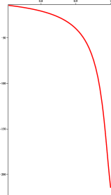
Figure 4.1. Graphic of $D_{3}$ for $L=2\pi$.

The Index Theorem, (see (1.30)) finally yield

$$\text{n}(\mathcal{L}_{3\Pi})=1-1-0=0\quad\mbox{and}\quad\text{z}(\mathcal{L}_{3\Pi})=1+0=1.$$

Hence, we have proved the following result.

Proposition 4.8.

For any $\omega\in(0,+\infty)$, the operator $\mathcal{L}_{{3\Pi}}$ defined in (1.29) has no negative eigenvalue. In addition, zero is a simple eigenvalue with eigenfunction $\varphi$.

5. Orbital instability of the cnoidal waves for the KG equation

The goal of this section is to establish a result of orbital instability based on the classical theory contained in [19] for the periodic traveling wave solutions $\varphi$ in $(\ref{cnoidal})$ for the KG equation (1.2). Consider the restricted energy space $X:=H_{per,m}^{1}\times L_{per,m}^{2}$. It is well known that (1.1) is invariant by translations. Thus, we can define for $x,r\in\mathbb{R}$ and $U=(u,v)\in X$

$$\mathrm{T}_{r}U(x)=(u(x+r),v(x+r)).$$

In what follows, for $c\in(-1,1)$, we define

$$\Phi:=(\varphi,c\varphi^{\prime}).$$

Next we recall the definition of the orbital stability in this context.

Definition 5.1 (Orbital Stability).

The periodic wave $\Phi$ is said orbitally stable if for all $\varepsilon>0$ there exists $\delta>0$ with the following property: if

$$\|(u_{0},v_{0})-(\varphi,c\varphi^{\prime})\|_{X}<\delta$$

and $U=(u,u_{t})$ is the weak solution of (1.1) in the interval $[0,t_{0})$, for some $t_{0}>0$, with $U(0)=(u_{0},v_{0})$, then $U$ can be continued to a solution in $0\leq t<\infty$ and

$$\sup_{t\in\mathbb{R}_{+}}\inf_{s\in\mathbb{R}}\big{\|}U(t)-\mathrm{T}_{s}\Phi\big{\|}_{X}<\varepsilon.$$

Otherwise, $\Phi$ is said to be orbitally unstable. In particular, this would happen in the case of solutions that cannot be continued.

Before establishing our orbital instability result, we present some additional results concerning the existence of weak solutions for Cauchy problem associated with (1.1) using the well known Potential Well Theory (for further details, see [31, Chapter 1] and [44]). First of all, for $\omega=1-c^{2}>0$ fixed, consider

$$P_{\omega}(u)=\frac{1}{2}\int_{0}^{L}(\omega u_{x}^{2}+u^{2})dx-\frac{1}{4}\int_{0}^{L}u^{4}dx,$$ (5.1)

where $u\in H_{per,m}^{1}$. For a fixed $L>0$, the critical points of $P_{\omega}$ in $H_{per,m}^{1}$ are unique and given in terms of cnoidal solutions as in $(\ref{cnoidal})$. Related to the functional $P_{\omega}$ in $(\ref{Ju})$, we have the Nehari manifold

$$\mathcal{N}=\left\{u\in H_{per,m}^{1}\backslash\{0\};\ \int_{0}^{L}(\omega u_{x}^{2}+u^{2})dx=\int_{0}^{L}u^{4}dx\right\}.$$

It is not difficult to show that $P_{\omega}$ satisfies the assumptions of the Mountain Pass Theorem (see e.g. [46]). In addition,

$$d_{\omega}:=\inf_{v\in H_{per,m}^{1}\backslash\{0\}}\max_{t\geq 0}P_{\omega}(tv),$$

is a critical level for the functional $P_{\omega}$. By using classical results in [46, Chapter 4], we obtain

$$d_{\omega}=\min_{u\in\mathcal{N}}P_{\omega}(u)=P_{\omega}(\varphi_{\omega}).$$ (5.2)

Concerning the cnoidal waves in $(\ref{Sol2})$, we obtain after some calculations that

$$P_{\omega}(\varphi_{\omega})=-\frac{L(K(k)-2)\left(\left(k^{4}-\frac{5}{3}k^{2}+\frac{2}{3}\right)K(k)+E(k)\left(\frac{4}{3}k^{2}-\frac{2}{3}\right)\right)}{K(k)(2k^{2}-1)^{2}}=\sqrt{\omega}P_{1}(\varphi_{1}),$$ (5.3)

where $k\in\left(\frac{1}{\sqrt{2}},1\right)$. In addition, by (5.3) it follows that $P_{\omega}(\varphi_{\omega})=0$ if and only if $K(k)-2=0$, that is, if and only if

$$k=k_{1}:\approx 0.802.$$ (5.4)

Since $\lim_{k\rightarrow\frac{1}{\sqrt{2}}^{+}}P_{\omega}(\varphi_{\omega})=+\infty$, we see for a fixed $k\in\left(\frac{1}{\sqrt{2}},k_{1}\right)$ that $P_{\omega}(\varphi_{\omega})>0$ is finite. As a consequence, by $(\ref{d1})$ we have $P_{\omega}(\varphi_{\omega})\leq P_{1}(\varphi_{1})$, so that $d_{\omega}=\sqrt{\omega}d_{1}\leq d_{1}$ for all $k\in\left(\frac{1}{\sqrt{2}},k_{1}\right)$ .
In this case, let us define

$$W_{\omega}=\{u\in H_{per,m}^{1};\ P_{\omega}(u)<d_{\omega}\}$$ (5.5)

and

$$W_{1,\omega}=\left\{u\in W_{\omega};\ \int_{0}^{L}(\omega u_{x}^{2}+u^{2})dx>\frac{1}{2}\int_{0}^{L}u^{4}dx\right\}\cup\{0\}.$$ (5.6)

We have the following well-posedness result.

Theorem 5.2.

The Cauchy problem associated with (1.1) is globally well-posed in $X$ in the following sense: for each initial data $u_{0}\in W_{1,\omega}$ and $v_{0}\in L_{per,m}^{2}$ satisfying

$$\frac{1}{2}||v_{0}||_{L_{per}^{2}}^{2}+P_{1}(u_{0})<d_{\omega},$$

there exists a unique (weak) solution $u$ for the equation (1.2) and satisfying $u\in C([0,T];H_{per,m}^{1})$ and $u_{t}\in C([0,T];L_{per,m}^{2})$ for all $T>0$.

Proof.

By using Galerkin’s method, the proof can be done using similar arguments in [31, Chapter 1, page 32] and it gives the existence of a weak solution $u\in L^{\infty}(0,T;H_{per,m}^{1})$ and $u_{t}\in L^{\infty}(0,T;L_{per,m}^{2})$ for all $T>0$. In fact, for the case $\omega=1$ the proof follows identical. For the case $\omega\in(0,1)$, we need some slight modifications. The a priori estimate to obtain the existence of global solutions in time is given by

$$\begin{array}[]{lllll}\displaystyle\frac{1}{2}||u_{x}(t)||_{L_{per}^{2}}^{2}&=&\displaystyle E(u_{0},v_{0})-\displaystyle\frac{1}{2}||u(t)||_{L_{per}^{2}}^{2}-\frac{1}{2}||u_{t}(t)||_{L_{per}^{2}}^{2}+\frac{1}{4}||u(t)||_{L_{per}^{4}}^{4}\\ \\ &<&\displaystyle E(u_{0},v_{0})+\frac{\omega}{2}||u_{x}(t)||_{L_{per}^{2}}^{2},\end{array}$$ (5.7)

where we are using the fact that $u_{0}\in W_{1,\omega}$ implies that $u(t)\in W_{1,\omega}$ a.e. $t\geq 0$. Since $||u_{x}(t)||_{L_{per}^{2}}<\frac{1}{\sqrt{1-\omega}}\sqrt{2E(u_{0},v_{0})}$ a.e. $t\geq 0$, it follows by the Poincaré-Wirtinger inequality and the Sobolev embedding $H_{per}^{1}\hookrightarrow L_{per}^{4}$ that $u\in L^{\infty}(0,T;H_{per,m}^{1})$ and $u_{t}\in L^{\infty}(0,T;L_{per,m}^{2})$ for all $T>0$. The uniqueness can be obtained by standard arguments and a Gronwall-type inequality. This fact enables us to conclude that $E(u,u_{t})=E(u_{0},v_{0})$ and $F(u,u_{t})=F(u_{0},v_{0})$ for all $t\in[0,T]$, so that both $u$ and $u_{t}$ are continuous in time as required. ∎

5.1. Instability for the cnoidal wave.

Let $L>0$ be fixed. For $c\in(-1,1)$, let us consider the cnoidal wave $\varphi$ given by $(\ref{cnoidal})$. The existence of the smooth curve $c\in I=(-1,1)\longmapsto\varphi_{c}$ given in Proposition 3.1 allows to define the function $\mathsf{d}:I\subset\mathbb{R}\longrightarrow\mathbb{R}$ given by $\mathsf{d}(c)=E(\varphi,c\varphi^{\prime})-cF(\varphi,c\varphi^{\prime})$. As we already pointed out in the introduction, we have

$$\begin{array}[]{lllll}\mathsf{d}^{\prime\prime}(c)=\displaystyle-\int_{0}^{L}(\varphi^{\prime}(x))^{2}dx+2(1-\omega)\frac{d}{d\omega}\int_{0}^{L}(\varphi^{\prime}(x))^{2}dx.\end{array}$$ (5.9)

Now, using the explicit expressions in Remark 3.4 and formulas $(312.02),$ $(312.04)$ and $(361.02)$ of [8], we obtain that

$$\int_{0}^{L}(\varphi^{\prime}(x))^{2}dx = \frac{2k^{2}}{2k^{2}-1}\frac{4{\rm\,K}(k)}{L}\int_{0}^{4{\rm\,K}(k)}{\rm sn}^{2}(u,k){\rm dn}^{2}(u,k)\;du$$

$$= \frac{32{\rm\,K}(k)}{3(2k^{2}-1)L}\Big{(}(2k^{2}-1){\rm\,E}(k)+(1-k^{2}){\rm\,K}(k)\Big{)},$$

In addition, since $\omega$ is a function of $k$, by (5.9) and the chain rule we have

$$\begin{array}[]{llllll}\mathsf{d}^{\prime\prime}(c)&=&\displaystyle-\int_{0}^{L}(\varphi^{\prime}(x))^{2}dx+2(1-\omega)\frac{d}{dk}\int_{0}^{L}(\varphi^{\prime}(x))^{2}dx\,\left(\frac{d\omega}{dk}\right)^{-1}\\ &&\\ &=&\displaystyle\frac{-32{\rm\,K}(k)}{3(2k^{2}-1)L}\Big{(}(2k^{2}-1){\rm\,E}(k)+(1-k^{2}){\rm\,K}(k)\Big{)}+\\ &&\\ &&\displaystyle+\frac{64(1-\omega)}{3L}\frac{d}{dk}\left(\frac{{\rm\,K}(k)}{(2k^{2}-1)}\Big{(}(2k^{2}-1){\rm\,E}(k)+(1-k^{2}){\rm\,K}(k)\Big{)}\right)\left(\frac{d\omega}{dk}\right)^{-1}.\\ \end{array}$$ (5.10)

In $(\ref{dc2})$, we denote

$$m(k):=\frac{-32{\rm\,K}(k)}{3(2k^{2}-1)L}\left((2k^{2}-1){\rm\,E}(k)+(1-k^{2}){\rm\,K}(k)\right)$$

and

$$n(k):=\frac{64(1-\omega)}{3L}\frac{d}{dk}\left(\frac{K(k)}{(2k^{2}-1)}\Big{(}(2k^{2}-1)E(k)+(-k^{2}+1)K(k)\Big{)}\right)\left(\frac{d\omega}{dk}\right)^{-1}.$$

After some algebraic calculations (see Figure 5.1), we see that $m(k)$ and $n(k)$ satisfies

$$m(k)+n(k)<0,\;\text{for all}\;k\in\left(\frac{1}{\sqrt{2}},1\right)$$

so that $\mathsf{d}^{\prime\prime}(c)<0,$ for $c\in[0,1)$.

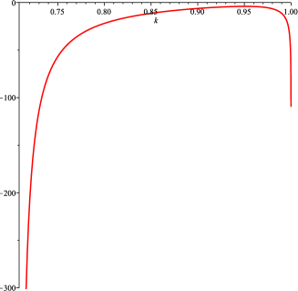
Figure 5.1. Graphic of $\mathsf{d}^{\prime\prime}$ as a function of $k\in\left(\frac{1}{\sqrt{2}},1\right)$.

Analysis above gives the following orbital instability result.

Theorem 5.3 (Orbital instability of the cnoidal waves for the KG equation).

Let $L>0$ be fixed. If $c\in[0,c(k_{1}))$, where $k_{1}$ is given in (5.4) and $\varphi$ is the cnoidal solution given in Proposition 3.1, then the periodic wave $\Phi$ is orbitally unstable in $X$ in the sense of Definition 5.1.

Proof.

By Proposition 4.5, there exists only one negative eigenvalue for the operator $\mathcal{L}_{\Pi}$ and it results to be simple. In addition, zero is a simple eigenvalue associated to the eigenfunction $(\varphi^{\prime},c\varphi^{\prime\prime})$. The result then follows from [19, Theorem 4.7] and the fact that $\mathsf{d}^{\prime\prime}(c)<0$ for all $c\in[0,c(k_{1}))\subset[0,c^{\ast})$. ∎

6. Orbital stability of the cnoidal waves for the NLS equation

The goal of this section is to establish a result of orbital stability, based on the Lyapunov functional arguments contained in [36] (see also [43]), for the periodic standing waves solutions for the NLS equation of the form (1.22), where $\omega\in(0,\omega^{*})$ is given in Proposition 4.7 and $\varphi:=\varphi_{\omega}$ given by Proposition 3.3.

Equation (1.2) has two basic symmetries, namely, translation and rotation. In other words, if $u=u(x,t)$ is a solution of (1.2), so are $e^{-i\theta}u$ and $u(x-r,t)$ for any $\theta,r\in\mathbb{R}$. By writing $U=P+iQ\equiv(P,Q)$ this is equivalent to saying that (1.2) is invariant by the transformations

$$T_{1}(\theta)U:=\left(\begin{array}[]{cc}\cos{\theta}&\sin{\theta}\\ -\sin{\theta}&\cos{\theta}\end{array}\right)\left(\begin{array}[]{c}P\\ Q\end{array}\right)$$

and

$$T_{2}(r)U:=\left(\begin{array}[]{c}P(\cdot-r,\cdot)\\ Q(\cdot-r,\cdot)\end{array}\right).$$

The actions $T_{1}$ and $T_{2}$ define unitary groups in $\mathbb{H}^{1}_{per,m}$ with infinitesimal generators given by

$$T_{1}^{\prime}(0)U:=\left(\begin{array}[]{cc}0&1\\ -1&0\end{array}\right)\left(\begin{array}[]{c}P\\ Q\end{array}\right)=J\left(\begin{array}[]{c}P\\ Q\end{array}\right)$$

and

$$T_{2}^{\prime}(0)U:=\partial_{x}\left(\begin{array}[]{c}P\\ Q\end{array}\right).$$

A standing wave solution as in (1.22) is then of the form

$$U(x,t)=\left(\begin{array}[]{c}\varphi(x)\cos(\omega t)\\ \varphi(x)\sin(\omega t)\end{array}\right).$$

Taking into account that the NLS equation is invariant by the actions of $T_{1}$ and $T_{2}$, we define the orbit generated by $\Phi=(\varphi,0)$ as

$$\Omega_{\Phi}=\big{\{}T_{1}(\theta)T_{2}(r)\Phi;\theta,r\in{\mathbb{R}}\big{\}}\equiv\left\{\left(\begin{array}[]{cc}\cos{\theta}&\sin{\theta}\\ -\sin{\theta}&\cos{\theta}\end{array}\right)\left(\begin{array}[]{c}\varphi(\cdot-r)\\ 0\end{array}\right)\;;\;\theta,r\in{\mathbb{R}}\right\}.$$

In $\mathbb{H}^{1}_{per,m}$, we introduce the pseudometric $d$ by

$$d(f,g):=\inf\{\|f-T_{1}(\theta)T_{2}(r)g\|_{\mathbb{H}^{1}_{per}}\;;\;\,\theta,r\in{\mathbb{R}}\}.$$

In particular, the distance between $f$ and $g$ is the distance between $f$ and the orbit generated by $g$ under the action of rotation and translation. In particular, $d(f,\Phi)=d(f,\Omega_{\Phi}).$

We present now our notion of orbital stability.

Definition 6.1.

Let $\Theta(x,t)=(\varphi(x)\cos(\omega t),\varphi(x)\sin(\omega t))$ be a standing wave for (1.19), where $\omega\in(0,+\infty)$. We say that $\Theta$ is orbitally stable in $\mathbb{H}^{1}_{per,m}$ provided that, given $\varepsilon>0$, there exists $\delta>0$ with the following property: if $U_{0}\in\mathbb{H}^{1}_{per,m}$ satisfies $\|U_{0}-\Phi\|_{\mathbb{H}^{1}_{per}}<\delta$, then the weak solution $U(t)$ for (1.19) with initial data $U_{0}$ exists for all $t\geq 0$ in $\mathbb{H}^{1}_{per,m}$ and satisfies

$$d(U(t),\Omega_{\Phi})<\varepsilon,\;\text{for all}\;t\geq 0.$$

Otherwise, we say that $\Theta$ is orbitally unstable in $\mathbb{H}^{1}_{per,m}$.

6.1. Global well-posedness

The first step to obtain the orbital stability is to show the global existence of weak solutions in $H_{per,m}^{1}$, which we give next.

Theorem 6.2.

The initial-value problem associated with (1.2) is globally well-posed in $H^{1}_{per,m}$. More precisely, for any $u_{0}\in H^{1}_{per,m}$ and any $T>0$, there exists a unique global (weak) solution of (1.2) in the sense that

$$u\in L^{\infty}(0,T;H^{1}_{per,m}),\,\,u_{t}\in L^{\infty}(0,T;H^{-1}_{per,m}),$$ (6.1)

and $u$ satisfies,

$$i\langle u_{t}(\cdot,t),\phi\rangle_{H^{-1}_{per,m},H_{per,m}^{1}}-\int_{0}^{L}u_{x}(\cdot,t)\overline{\phi_{x}}\;dx+\int_{0}^{L}u(\cdot,t)|u(\cdot,t)|^{2}\overline{\phi}\;dx=0,\,\mbox{ a.e. }t\in[0,T],$$ (6.2)

for all $\phi\in H^{1}_{per,m}$. Furthermore, $u$ satisfies $u(\cdot,0)=u_{0}$ and there exist constants $c_{1},c_{2}>0$ such that

$$\mathcal{E}(u(\cdot,t))\equiv c_{1}\,\mbox{ and }\,\mathcal{F}(u(\cdot,t))\equiv c_{2},\,\,\mbox{ a.e. }t\in[0,T],$$ (6.3)

where $\mathcal{E}$ and $\mathcal{F}$ are defined in (1.20) and (1.21). Equalities in $(\ref{conserv})$ allow to conclude from $(\ref{cond1})$ that

$$u\in C([0,T];H^{1}_{per,m}),\,\,u_{t}\in C([0,T];H^{-1}_{per,m}).$$ (6.4)

Proof.

To prove this result, we use Galerkin’s method. Since the method is quite well-known we give only the main steps (for some additional details, see the Appendix). Let $\{w_{j}\}_{j\in\mathbb{Z}\backslash\{0\}}$ be the sequence given by

$$w_{j}(x)=\frac{1}{\sqrt{L}}e^{\frac{2\pi i}{L}jx},$$

which is a complete orthonormal set in $L^{2}_{per,m}$ and orthogonal in $H^{1}_{per,m}$.

Let $T>0$ be arbitrary but fixed. For each positive integer $n$, let $V_{n}$ be the finite subspace generated by $w_{-n},w_{-n+1},\ldots,w_{n}$. By using the Carathéodory Theorem ([9, Chapter 2, Theorem 1.1] and [15, Chapter 1]), we can show the existence of functions $g_{jn}$ such that the function

$$u_{n}(t)=\sum_{{{j=-n}}\atop{j\neq 0}}^{n}g_{jn}(t)w_{j}\in V_{n},$$

satisfies, for each $j\in\{-n,\ldots,-1,1,\ldots n\}$, the following approximate problem

$$\left\{\begin{array}[]{llll}\displaystyle i\langle u_{n,t}(t),w_{j}\rangle_{H_{per,m}^{-1},H_{per,m}^{1}}-\int_{0}^{L}u_{n,x}(\cdot,t)\overline{w_{j,x}}dx+\int_{0}^{L}u_{n}(\cdot,t)|u_{n}(\cdot,t)|^{2}\overline{w_{j}}dx=0,\\ \\ u_{n}(0)=u_{0n}=\displaystyle{\sum_{{{j=-n}}\atop{j\neq 0}}^{n}(u_{0},w_{j})_{{H}^{1}_{per}}w_{j}}\longrightarrow u_{0}\mbox{ in }H^{1}_{per,m},\;\text{as}\;n\to\infty\end{array}\right.$$ (6.5)

for all $t\in[0,T]$. Note that a priori estimates allow us to define functions $u_{n}(t)$ in the interval $[0,T]$. Since $w_{j}\in H^{1}_{per,m}$ for all $j\in\mathbb{Z}\backslash\{0\}$ and $H^{1}_{per,m}$ is a closed subspace of $H^{1}_{per}$, we obtain all standard steps concerning Galerkin’s method and the proof of the theorem follows. ∎

6.2. Positivity of the operator $\boldsymbol{\mathcal{G}^{\prime\prime}(\Phi)}$

In this section our goal is to study the positivity of the operator $\mathcal{G}^{\prime\prime}(\Phi)$ given in (1.26). Before that, we need to prove some positivity properties for the operators $\mathcal{L}_{2}$ and $\mathcal{L}_{3}$ in (1.27).

Lemma 6.3.

There exists $\delta_{2}>0$ such that

$$(\mathcal{L}_{3\Pi}\,v,v)_{L^{2}_{per}}\geq\delta_{2}\|v\|_{L^{2}_{per}}^{2},$$ (6.6)

for all $v\in H^{2}_{per,m}$ satisfying $(v,\varphi)_{L^{2}_{per}}=0$.

Proof.

Since $L^{2}_{per,m}$ is a Hilbert space and $\varphi\in L^{2}_{per,m}$, we have the decomposition $L^{2}_{per,m}=N\oplus M,$ where $N:=[\varphi]$ and $M:=[\varphi]^{\perp}$. From Theorem 6.17 in [29, page 178], we obtain

$$\sigma\left(\mathcal{L}_{3\Pi}\right)=\sigma\left(\mathcal{L}_{3\Pi,N}\right)\cup\sigma\left(\mathcal{L}_{3\Pi,M}\right),$$

where $\mathcal{L}_{3\Pi,N}$ and $\mathcal{L}_{3\Pi,M}$ denote the operator $\mathcal{L}_{3\Pi}$ restricted to $N$ and $M$, respectively, and $\sigma(\mathcal{A})$ denotes the spectrum of the linear operator $\mathcal{A}$. Since $\text{Ker}(\mathcal{L}_{3\Pi})=[\varphi]$, we obtain

$$\sigma\left(\mathcal{L}_{3\Pi,M}\right)=\sigma\left(\mathcal{L}_{3\Pi}\right)\setminus\{0\},$$

that is, the spectrum of $\mathcal{L}_{3\Pi,M}$ is bounded from below. The arguments in [29, page 278], imply that $\mathcal{L}_{3\Pi}$ is also bounded from below, so that there exists $\delta_{2}>0$ satisfying

$$(\mathcal{L}_{3\Pi}\,v,v)_{L^{2}_{per}}\geq\delta_{2}\|v\|_{L^{2}_{per}},\,\,\text{for all}\,v\in M\cap H^{2}_{per,m},$$

Therefore, for all $v\in H^{2}_{per,m}$ such that $(v,\varphi)_{L^{2}_{per}}=0$ we have that (6.6) holds. ∎

Before proving the next result, we recall the convexity of the function $\mathsf{d}$ defined by $\mathsf{d}(\omega)=\mathcal{G}(\Phi)=\mathcal{E}(\Phi)+\omega\mathcal{F}(\Phi)$.

Proposition 6.4.

Let $L>0$ be fixed. For the cnoidal wave $\varphi$ given by Proposition 3.3, we have $\mathsf{d}^{\prime\prime}(\omega)>0$ for all $\omega\in(0+\infty)$.

Proof.

See [2, page 23]. ∎

Next result gives us that the quadratic form associated to the operator $\mathcal{L}_{2\Pi}$ is non-negative when restricted to $[\varphi]^{\perp}$.

Lemma 6.5.

Let $\gamma$ be defined as

$$\gamma:=\inf\left\{(\mathcal{L}_{2\Pi}\,v,v)_{L^{2}_{per}}:v\in H^{2}_{per,m},\,(v,\varphi)_{L^{2}_{per}}=0,\,\|v\|_{L^{2}_{per}}=1\right\}.$$ (6.7)

Then $\gamma=0$.

Proof.

Let us define

$$\gamma_{0}:=\inf\left\{\langle\mathcal{L}_{2\Pi}v,v\rangle:v\in H^{1}_{per,m},\,(v,\varphi)_{L^{2}_{per}}=0,\,\|v\|_{L^{2}_{per}}=1\right\},$$ (6.8)

where $\langle\cdot,\cdot\rangle:=\langle\cdot,\cdot\rangle_{H^{-1}_{per,m},H^{1}_{per,m}}$. Let us first prove that $\gamma_{0}=0$ and the infimum in (6.8) is achieved. In fact, since $\varphi$ is periodic, we have

$$\langle\mathcal{L}_{2\Pi}v,v\rangle =\|v^{\prime}\|_{L^{2}_{per}}+\omega-3(\varphi^{2},v^{2})_{L^{2}_{per}}\geq-3\,(\varphi^{2},v^{2})_{L^{2}_{per}}\geq-3\,\|\varphi^{2}\|_{L^{\infty}_{per}},$$

for all $v\in H^{1}_{per,m}$ such that $\|v\|_{L^{2}_{per}}=1$. This implies that $\gamma_{0}$ is finite. Furthermore, since $(\varphi,\varphi^{\prime})_{L^{2}_{per}}=0$ and $\mathcal{L}_{2\Pi}\varphi^{\prime}=0$ we get $\gamma_{0}\leq 0.$

Now, we prove that the infimum in (6.8) is achieved. Indeed, let $\{u_{j}\}_{j\in\mathbb{N}}\subset H^{1}_{per,m}$ be a sequence such that

$$\|u_{j}\|_{L^{2}_{per}}=1,\,\,\,(u_{j},\varphi)_{L^{2}_{per}}=0,\;\text{for all}\;j\in\mathbb{N}\,\mbox{ and }\,\langle\mathcal{L}_{2\Pi}u_{j},u_{j}\rangle\longrightarrow\gamma_{0},\;\text{as}\;j\rightarrow\infty.$$ (6.9)

Since the sequence $\left\{\langle\mathcal{L}_{2\Pi}u_{j},u_{j}\rangle\right\}_{j\in\mathbb{N}}$ is bounded in $\mathbb{R}$, there exists $C>0$ so that

$$\langle\mathcal{L}_{2\Pi}u_{j},u_{j}\rangle\leq C\;\text{for all}\;j\in\mathbb{N}.$$ (6.10)

Now, since $\varphi$ is bounded we obtain from $(\ref{est1})$ the existence of $C_{1}>0$ such that

$$\omega\|u_{j}\|_{L^{2}_{per}}^{2}+\|u_{j}^{\prime}\|_{L^{2}_{per}}^{2}=\langle\mathcal{L}_{2\Pi}u_{j},u_{j}\rangle+3(\varphi^{2},u_{j}^{2})_{L^{2}_{per}}\leq C_{1},\;\text{for all}\;j\in\mathbb{N},$$

which gives that $\{u_{j}\}_{j\in\mathbb{N}}$ is bounded in $H^{1}_{per,m}$. Hence, there exists a subsequence, still denoted by $\{u_{j}\}_{j\in\mathbb{N}}$ and $u\in H^{1}_{per,m}$ such that $u_{j}\rightharpoonup u\,\mbox{ in }\,H^{1}_{per,m}.$ By (6.9) and the compact embedding $H^{1}_{per,m}\hookrightarrow L^{2}_{per,m}$, we have $\|u\|_{L^{2}_{per}}=1\,\mbox{ and }\,(u,\varphi)_{L^{2}_{per}}=0.$ In addition, Fatou’s Lemma yields

$$\gamma_{0}\leq\langle\mathcal{L}_{2\Pi}\,u,u\rangle\leq\liminf_{j\in\mathbb{N}}\langle\mathcal{L}_{2\Pi}\,u_{j},u_{j}\rangle=\gamma_{0}.$$

Last inequality allows to deduce that the infimum in (6.8) is achieved at the function $u$.

It remains to prove that $\gamma_{0}\geq 0$. Let

$$\Upsilon_{0}:=\left\{v\in H^{1}_{per,m},\,(v,\varphi)_{L^{2}_{per}}=0,\,\|v\|_{L^{2}_{per}}=1\right\}.$$

It is then suffices to show

$$\langle\mathcal{L}_{2\Pi}v,v\rangle\geq 0,\;\text{for all}\;v\in\Upsilon_{0}.$$

For this, let us start by noting that if $\chi=-\dfrac{\partial\varphi}{\partial\omega}$ then $\mathcal{L}_{2}\chi=\varphi$, and

$$\langle\mathcal{L}_{2\Pi}\chi,\chi\rangle=\langle\mathcal{L}_{2}\chi,\chi\rangle=\left\langle\mathcal{L}_{2}\dfrac{\partial\varphi}{\partial\omega},\dfrac{\partial\varphi}{\partial\omega}\right\rangle=\left(\mathcal{L}_{2}\dfrac{\partial\varphi}{\partial\omega},\dfrac{\partial\varphi}{\partial\omega}\right)_{L^{2}_{per}}=-\left(\varphi,\dfrac{\partial\varphi}{\partial\omega}\right)_{L^{2}_{per}}=-\mathsf{d}^{\prime\prime}(\omega).$$ (6.11)

By Proposition 6.4, we have

$$\langle\mathcal{L}_{2\Pi}\chi,\chi\rangle<0.$$ (6.12)

Now, recall that $\text{Ker}(\mathcal{L}_{2\Pi})=[\varphi^{\prime}]$ and $\text{n}(\mathcal{L}_{2\Pi})=1.$ Then, there exists $-\lambda^{2}<0$ and $\Psi\in D(\mathcal{L}_{2\Pi})$ such that $\|\Psi\|_{L^{2}_{per}}=1$ and $\mathcal{L}_{2\Pi}\Psi=-\lambda^{2}\Psi.$ In addition we may write

$$L^{2}_{per,m}=[\Psi]\oplus[\varphi^{\prime}]\oplus P.$$

where $P\subset L^{2}_{per,m}$ is such that

$$\langle\mathcal{L}_{2\Pi}u,u\rangle\geq\delta\|u\|_{L^{2}_{per}}^{2},\;\text{for all}\;u\in\tilde{P}:=D(\mathcal{L}_{2\Pi})\cap P.$$

Next, since $\chi\in H_{per,m}^{1}$, we infer

$$\chi=a_{0}\Psi+b_{0}\varphi^{\prime}+p_{0},$$

where $a_{0},b_{0}\in\mathbb{R}$ and $p_{0}\in\tilde{P}$. By (6.12), we have

$$\begin{array}[]{llll}\langle\mathcal{L}_{2\Pi}p_{0},p_{0}\rangle&=\langle\mathcal{L}_{2\Pi}(\chi-a_{0}\Psi-b_{0}\varphi^{\prime}),\chi-a_{0}\Psi-b_{0}\varphi^{\prime}\rangle\\ &=\langle\mathcal{L}_{2\Pi}\chi,\chi\rangle+a_{0}^{2}\lambda^{2}\\ &<a_{0}^{2}\lambda^{2}.\end{array}$$ (6.13)

Let $v\in\Upsilon_{0}$ be arbitrary. First, if $v=\beta\varphi^{\prime}$, for some $\beta\neq 0$ then clearly

$$\langle\mathcal{L}_{2\Pi}\tilde{v},\tilde{v}\rangle=0,\qquad\tilde{v}=\frac{v}{\|v\|_{L^{2}_{per}}}\in\Upsilon_{0}.$$ (6.14)

On the other hand, if $v\notin[\varphi^{\prime}]$, there exist $a_{1},b_{1}\in{\mathbb{R}}$ and $p_{1}\in P$ such that

$$v=a_{1}\Psi+b_{1}\varphi^{\prime}+p_{1}.$$

Thus,

$$\begin{array}[]{llll}0=-(\varphi,v)_{L^{2}_{per}}&=\left(\mathcal{L}_{2\Pi}\chi,v\right)_{L^{2}_{per}}\\ &=\langle\mathcal{L}_{2\Pi}\chi,v\rangle\\ &=\langle-a_{0}\lambda^{2}\Psi+\mathcal{L}_{2\Pi}p_{0},a_{1}\Psi+b_{1}\varphi^{\prime}+p_{1}\rangle\\ &=-a_{0}a_{1}\lambda^{2}+\langle\mathcal{L}_{2\Pi}p_{0},p_{1}\rangle.\end{array}$$ (6.15)

Using the fact that $\xi(f,g)=\langle\mathcal{L}_{2\Pi}f,g\rangle$ defines a non-negative sesquilinear form on $\tilde{P}$, we obtain the Cauchy-Schwarz inequality:

$$|\xi(f,g)|^{2}\leq\langle\mathcal{L}_{2\Pi}f,f\rangle\,\langle\mathcal{L}_{2\Pi}g,g\rangle,\;\text{for all}\;f,g\in\tilde{P}.$$ (6.16)

Consequently, by (6.13), (6.15) and (6.16), we have

$$\langle\mathcal{L}_{2\Pi}v,v\rangle =\langle\mathcal{L}_{2\Pi}(a_{1}\Psi+b_{1}\varphi^{\prime}+p_{1}),a_{1}\Psi+b_{1}\varphi^{\prime}+p_{1}\rangle$$

$$=-a_{1}^{2}\lambda^{2}+\langle\mathcal{L}_{2\Pi}p_{1},p_{1}\rangle$$

$$\geq-a_{1}^{2}\lambda^{2}+\dfrac{|\langle\mathcal{L}_{2\Pi}p_{0},p_{1}\rangle|^{2}}{\langle\mathcal{L}_{2\Pi}p_{0},p_{0}\rangle}$$

$$>-a_{1}^{2}\lambda^{2}+\dfrac{a_{0}^{2}a_{1}^{2}\lambda^{4}}{a_{0}^{2}\lambda^{2}}$$

$$=0,$$

that is,

$$\langle\mathcal{L}_{2\Pi}v,v\rangle>0,\;\text{for all}\;v\in\Upsilon_{0}\ \mbox{with}\ v\notin[\varphi^{\prime}].$$ (6.17)

By (6.14) and (6.17) we obtain $\gamma_{0}\geq 0$.

In order to complete the proof of the lemma it suffices to show that $\gamma=\gamma_{0}$. To this end, take $u\in\Upsilon_{0}$ satisfying $\langle\mathcal{L}_{2\Pi}u,u\rangle=\gamma_{0}.$ From the Lagrange multiplier theorem there exist $\eta,\zeta\in{\mathbb{R}}$ such that

$$\mathcal{L}_{2\Pi}u=\eta u+\zeta\varphi.$$ (6.18)

We see by (6.18) that $u\in H^{2}_{per,m}$, which allows to conclude that $\gamma=\gamma_{0}=0$ and the proof of the lemma is completed. ∎

Lemma 6.6.

Let $\xi$ be defined as

$$\xi:=\inf\left\{(\mathcal{L}_{2\Pi}v,v)_{L^{2}_{per}}:v\in H^{2}_{per,m},\,(v,\varphi)_{L^{2}_{per}}=(v,\varphi^{\prime})_{L^{2}_{per}}=0,\,\|v\|_{L^{2}_{per}}=1\right\}.$$ (6.19)

Then $\xi>0$.

Proof.

From Lemma 6.5 it is clear that $\xi\geq 0$. Assume by contradiction that $\xi=0$. Using similar arguments as in Lemma 6.5 we may show that the infimum in (6.19) is attained at a function $u\in H^{2}_{per,m}$ satisfying

$$\|u\|_{L^{2}_{per}}=1,\,\,(u,\varphi)_{L^{2}_{per}}=(u,\varphi^{\prime})_{L^{2}_{per}}=0\ \mbox{and}\ (\mathcal{L}_{2\Pi}u,u)_{L^{2}_{per}}=\xi=0.$$ (6.20)

By the Lagrange multiplier theorem, there exist $\lambda,\theta,\nu\in{\mathbb{R}}$ such that

$$\mathcal{L}_{2\Pi}u=\lambda u+\theta\varphi+\nu\varphi^{\prime}.$$ (6.21)

From (6.20) and (6.21), we clearly have $\lambda=0$. Also, taking the inner product in (6.21) with $\varphi^{\prime}$ and taking into account that $\mathcal{L}_{2\Pi}$ is self-adjoint we deduce that $\nu=0$ and consequently $\mathcal{L}_{2\Pi}u=\theta\varphi$. Recalling that $\mathcal{L}_{2\Pi}\chi=\varphi$, where $\chi=-\dfrac{\partial\varphi}{\partial\omega}$, we have $\mathcal{L}_{2\Pi}(\theta\chi)=\theta\varphi=\mathcal{L}_{2\Pi}u$ which implies $\mathcal{L}_{2\Pi}(u-\theta\chi)=0.$ Since $\text{Ker}(\mathcal{L}_{2\Pi})=[\varphi^{\prime}]$, there exists $\sigma\in{\mathbb{R}}$ such that $u-\theta\chi=\sigma\varphi^{\prime}$. On the other hand, using that $(\chi,\varphi)_{L^{2}_{per}}=-\mathsf{d}^{\prime\prime}(\omega)<0$ (see (6.11)) and $(\varphi^{\prime},\varphi)_{L^{2}_{per}}=0$, we obtain by (6.20) that $-\theta(\chi,\varphi)_{L^{2}_{per}}=(\sigma\varphi^{\prime}-u,\varphi)_{L^{2}_{per}}=0,$ and hence $\theta=0$. Thus, we conclude that $u=\sigma\varphi^{\prime}$ for some $\sigma\neq 0$. But this is a contradiction because from (6.20), $0=(u,\varphi^{\prime})_{L^{2}_{per}}=\sigma\|\varphi^{\prime}\|_{L^{2}_{per}}\neq 0.$ ∎

Corollary 6.7.

Let $\mathcal{L}_{\Pi}:\mathbb{H}^{2}_{per,m}\subset\mathbb{L}^{2}_{per,m}\rightarrow\mathbb{L}^{2}_{per,m}$ be defined by

$$\mathcal{L}_{\Pi}:=\left(\begin{array}[]{cc}\mathcal{L}_{2\Pi}&0\\ 0&\mathcal{L}_{3\Pi}\end{array}\right),$$

where $\mathcal{L}_{2\Pi}$ and $\mathcal{L}_{3\Pi}$ are given in (1.28) and (1.29), respectively. If $f=(u,v)\in\mathbb{H}^{2}_{per,m}$ satisfies

$$(v,\varphi)_{L^{2}_{per}}=(u,\varphi)_{L^{2}_{per}}=(u,\varphi^{\prime})_{L^{2}_{per}}=0$$ (6.22)

then there exists $\delta>0$ such that

$$(\mathcal{L}_{\Pi}f,f)_{\mathbb{L}^{2}_{per}}\geq\delta\|f\|^{2}_{\mathbb{L}^{2}_{per}}.$$

Proof.

Let $f=(u,v)\in\mathbb{H}^{2}_{per,m}$ be satisfying (6.22). From Lemmas 6.3 and 6.6, there exist $\delta_{1},\delta_{2}>0$ such that

$$(\mathcal{L}_{2\Pi}\,u,u)_{L^{2}_{per}}\geq\delta_{1}\|u\|^{2}_{L^{2}_{per}}\,\,\mbox{ and }\,\,(\mathcal{L}_{3\Pi}\,v,v)_{L^{2}_{per}}\geq\delta_{2}\|v\|^{2}_{L^{2}_{per}}.$$

Thus,

$$(\mathcal{L}_{\Pi}f,f)_{\mathbb{L}^{2}_{per}}=(\mathcal{L}_{2\Pi}\,u,u)_{L^{2}_{per}}+(\mathcal{L}_{3\Pi}\,v,v)_{L^{2}_{per}}\geq\delta_{1}\|u\|^{2}_{L^{2}_{per}}+\delta_{2}\|v\|^{2}_{L^{2}_{per}}.$$

Defining $\delta:=\min\{\delta_{1},\delta_{2}\}>0$, the last inequality gives the desired. ∎

Lemma 6.8.

There exist positive constants $\alpha_{1}$ and $\alpha_{2}$ such that

$$(\mathcal{L}_{\Pi}f,f)_{\mathbb{L}^{2}_{per}}\geq\alpha_{1}\|f\|^{2}_{\mathbb{H}^{1}_{per}}-\alpha_{2}\|f\|^{2}_{\mathbb{L}^{2}_{per}},$$

for all $f=(u,v)\in\mathbb{H}^{2}_{per,m}$.

Proof.

Let $f=(u,v)\in\mathbb{H}^{2}_{per,m}$ be fixed. Since $\mathcal{L}_{2}$ and $\mathcal{L}_{3}$ are second order differential operators, we obtain from G$\mathring{\text{a}}$rding’s inequality (see [47, page 175]) that

$$(\mathcal{L}_{2\Pi}\,u,u)_{L^{2}_{per}}=(\mathcal{L}_{2}\,u,u)_{L^{2}_{per}}\geq\beta_{1}\|u\|_{H^{1}_{per}}^{2}-\beta_{2}\|u\|_{L^{2}_{per}}^{2}$$

and

$$(\mathcal{L}_{3\Pi}\,v,v)_{L^{2}_{per}}=(\mathcal{L}_{3}\,v,v)_{L^{2}_{per}}\geq\beta_{3}\|v\|_{H^{1}_{per}}^{2}-\beta_{4}\|v\|_{L^{2}_{per}}^{2}.$$

By setting $\alpha_{1}=\min\{\beta_{1},\beta_{3}\}>0$ and $\alpha_{2}=\max\{\beta_{2},\beta_{4}\}>0,$ we obtain

$$(\mathcal{L}_{\Pi}f,f)_{\mathbb{L}^{2}_{per}}=(\mathcal{L}_{2\Pi}\,u,u)_{L^{2}_{per}}+(\mathcal{L}_{3\Pi}\,v,v)_{L^{2}_{per}}\geq\alpha_{1}\|f\|^{2}_{\mathbb{H}^{1}_{per}}-\alpha_{2}\|f\|^{2}_{\mathbb{L}^{2}_{per}},$$

which completes the proof of the lemma. ∎

Remark 6.9.

Let $\omega>0$ be fixed. Recall that $\mathcal{G}:\mathbb{H}^{1}_{per}\rightarrow{\mathbb{R}}$ is given by $\mathcal{G}=\mathcal{E}+\omega\mathcal{F},$ and $\mathcal{G}^{\prime\prime}(\Phi):\mathbb{H}^{1}_{per}\rightarrow\mathbb{H}_{per}^{-1}.$ Let $\mathsf{b}:D(\mathsf{b})=\mathbb{H}^{3}_{per}\subset\mathbb{L}^{2}_{per}\rightarrow{\mathbb{R}}$ be the quadratic form associated to the operator $\mathcal{G}^{\prime\prime}(\Phi)$, that is,

$$\mathsf{b}(v)=\langle\mathcal{G}^{\prime\prime}(\Phi)v,v\rangle_{\mathbb{H}^{-1}_{per},\mathbb{H}^{1}_{per}}=(\mathcal{L}v,v)_{\mathbb{L}^{2}_{per}},\;\text{for all}\;v\in D(\mathsf{b}).$$

Note that $\mathsf{b}$ is densely defined and, from Lemma 6.8, $\mathsf{b}$ is closed and bounded from below. Thus, (see, for instance, [29, Theorem 2.6 and page 322]) we obtain that $\mathcal{L}$ is the unique self-adjoint linear operator such that

$$\langle\mathcal{G}^{\prime\prime}(\Phi)v,z\rangle_{\mathbb{H}^{-1}_{per},\mathbb{H}^{1}_{per}}=(\mathcal{L}v,z)_{\mathbb{L}^{2}_{per}}=(\mathcal{L}_{\Pi}v,z)_{\mathbb{L}^{2}_{per}},$$

for all $v\in\mathbb{H}^{3}_{per,m}$ and $z\in\mathbb{H}^{1}_{per,m}$. In this case, if $\mathcal{I}:\mathbb{H}^{1}_{per}\rightarrow\mathbb{H}^{-1}_{per}$ is the natural injection of $\mathbb{H}^{1}_{per}$ into $\mathbb{H}^{-1}_{per}$ with respect to the inner product in ${\mathbb{L}^{2}}$, that is,

$$\langle\mathcal{I}u,v\rangle_{\mathbb{H}^{-1},\mathbb{H}^{1}}=(u,v)_{\mathbb{L}^{2}_{per}},\;\text{for all}\;u,v\in\mathbb{H}^{1}_{per},$$

then

$$\mathcal{G}^{\prime\prime}(\Phi)v=\mathcal{I}\mathcal{L}v,\;\text{for all}\;v\in\mathbb{H}^{3}_{per,m}.$$

Since $H^{1}_{per,m}\hookrightarrow H^{1}_{per}$ and $H^{-1}_{per}\hookrightarrow H^{-1}_{per,m}$, we can write $\mathcal{I}:\mathbb{H}^{1}_{per,m}\rightarrow\mathbb{H}^{-1}_{per,m}$ as

$$\langle\mathcal{I}u,v\rangle_{\mathbb{H}^{-1}_{per,m},\mathbb{H}^{1}_{per,m}}=\langle\mathcal{I}u,v\rangle_{\mathbb{H}_{per}^{-1},\mathbb{H}_{per}^{1}}=(u,v)_{\mathbb{L}^{2}_{per}},\;\text{for all}\;u,v\in\mathbb{H}^{1}_{per,m}.$$

With the above identification in mind, we may prove the following.

Lemma 6.10.

There exists $\delta^{*}>0$ such that

$$\langle\mathcal{G}^{\prime\prime}(\Phi)f,f\rangle_{\mathbb{H}^{-1}_{per},\mathbb{H}^{1}_{per}}\geq\delta^{*}\|f\|_{\mathbb{H}^{1}_{per}}^{2},$$ (6.23)

for all $f=(u,v)\in\mathbb{H}^{1}_{per,m}$ satisfying (6.22)

Proof.

Assume first that $f=(u,v)\in\mathbb{H}^{3}_{per,m}$ satisfies (6.22). By Corollary 6.7, we have

$$\frac{1}{\delta}(\mathcal{L}_{\Pi}f,f)_{\mathbb{L}^{2}_{per}}\geq\|f\|_{\mathbb{L}^{2}_{per}}^{2}.$$

So, by Lemma 6.8, we obtain

$$(\mathcal{L}_{\Pi}f,f)_{\mathbb{L}^{2}_{per}}\geq\alpha_{1}\|f\|_{\mathbb{H}^{1}_{per}}^{2}-\alpha_{2}\|f\|_{\mathbb{L}^{2}_{per}}^{2}\geq\alpha_{1}\|f\|_{\mathbb{H}^{1}_{per}}^{2}-\frac{\alpha_{2}}{\delta}(\mathcal{L}_{\Pi}f,f)_{\mathbb{L}^{2}_{per}},$$

implying that

$$\left(1+\dfrac{\alpha_{2}}{\delta}\right)(\mathcal{L}_{\Pi}f,f)_{\mathbb{L}^{2}_{per}}\geq\alpha_{1}\|f\|_{\mathbb{H}^{1}_{per}}^{2}.$$

Defining $\delta^{*}:=\dfrac{\alpha_{1}\delta}{\alpha_{2}+\delta}>0$ we see that (6.23) holds for any $f\in\mathbb{H}^{3}_{per,m}$. By density, we obtain the desired result. ∎

6.3. Stability of the cnoidal waves

Notice that Lemma 6.10 establishes the positivity of $\mathcal{G}^{\prime\prime}(\Phi)$ under the orthogonality condition (6.22), which holds in $L^{2}_{per}$. However, this is enough to obtain the same positivity under the orthogonality condition in $H^{1}_{per}$ (see [36, Section 4]). This allows to show that, for some positive constant $M$, the function

$$V(v)=\mathcal{E}(v)-\mathcal{E}(\Phi)+M\left(\mathcal{F}(v)-\mathcal{F}(\Phi)\right)^{2}$$

is a suitable Lyapunov function for the orbit $\Omega_{\Phi}$. With such a function in hand, we are able to prove the following.

Theorem 6.11 (Orbital stability of the cnoidal waves for the NLS equation).

Let $L>0$ be fixed. If $\omega\in(0,\omega^{*})$, where $\omega^{*}$ is given in Proposition 4.7 and $\varphi=\varphi_{\omega}$ is the cnoidal solution given in Proposition 3.3 then the standing wave

$$\Theta(x,t):=\begin{pmatrix}\varphi(x)\cos(\omega t)\\ \varphi(x)\sin(\omega t)\end{pmatrix}$$

is orbitally stable in $\mathbb{H}^{1}_{per,m}$ in the sense of Definition 6.1.

Since the proof is similar to that of Theorem 4.17 in [36] we omit the details.

Appendix - The Galerkin method and the existence of global weak solutions

In this appendix we present some complementary facts concerning the Galerkin approximation used in the proof of Theorem 6.2 (and Theorem 5.2). Since the existence of global solutions is a crucial step in order to apply the stability method as showed in Section 6, we only present the additional facts for the equation $(\ref{KF1})$. Similar arguments can be done for equation $(\ref{KF2})$, but it is important to mention that the orbital instability in Section 5 can be determined using the existence of local solutions. Global solutions are not necessary in that case.

I - A priori estimates. Replacing $w_{j}$ by $u_{n}(t)\in V_{n}$ in the approximate problem $(\ref{approblem})$, we obtain after some basic calculations (well known in the case of NLS) that

$$||u_{n}(t)||_{L_{per}^{2}}^{2}=||u_{0n}||_{L_{per}^{2}}^{2},$$ (6.24)

for all $t\in[0,t_{n}]$, where $t_{n}$ is the maximum time of existence obtained by Caratheodory’s Theorem. On the other hand, replacing $w_{j}$ by $u_{n,t}(t)\in V_{n}$ in the same problem, we also obtain

$$\mathcal{E}(u_{m}(t))=\mathcal{E}(u_{0n}),$$ (6.25)

for all $t\in[0,t_{n}]$, where $\mathcal{E}$ is defined as in $(\ref{quantEF1})$. These a priori estimates allows to extend the solution $u_{n}(t)$ to the whole interval $[0,T]$. Thus, using $(\ref{est12})$ and $(\ref{est13})$ combined with the Gagliardo-Nirenberg inequality for periodic domains, we obtain

$$||u_{n,x}(t)||_{L_{per}^{2}}^{2}\leq 2\mathcal{E}(u_{0n})+C||u_{n,x}(t)||_{L_{per}^{2}}||u_{n0}||_{L_{per}^{2}}^{3}+C||u_{n0}||_{L_{per}^{2}}^{4}.$$ (6.26)

Combining $(\ref{est12})$ and $(\ref{est14})$, it follows that for each $T>0$, we have

$$\{u_{n}\}\ \mbox{is bounded in}\ L^{\infty}(0,T;H_{per,m}^{1}),$$ (6.27)

for all $n\in\mathbb{Z}\backslash\{0\}$.
Next, using a standard argument of duality, we also obtain

$$\{u_{n,t}\}\ \mbox{is bounded in}\ L^{\infty}(0,T;H_{per,m}^{-1}),$$ (6.28)

for all $n\in\mathbb{Z}\backslash\{0\}$.
II - Passage to the limit. Using $(\ref{est15})$ and $(\ref{est16})$, we obtain in particular that

$$\{u_{n}\}\ \mbox{is bounded in}\ L^{2}(0,T;H_{per,m}^{1}),$$ (6.29)

and

$$\{u_{n,t}\}\ \mbox{is bounded in}\ L^{2}(0,T;H_{per,m}^{-1}),$$ (6.30)

for all $n\in\mathbb{Z}\backslash\{0\}$.
Thus, up to a subsequence, the following basic convergences are obtained

$$\displaystyle\begin{array}[]{llll}u_{n}\rightharpoonup u\ \ \ \textrm{weak in\ }\ \ L^{2}(0,T;H^{1}_{per,m}),\\ u_{n,t}\rightharpoonup u_{t}\ \ \ \textrm{weak in\ }\ \ L^{2}(0,T;H^{-1}_{per,m}),\\ u_{n}\stackrel{{\scriptstyle\star}}{{\rightharpoonup}}u\ \ \ \textrm{weak-$*$ in\ }\ \ L^{\infty}(0,T;H^{1}_{per,m}),\\ u_{n,t}\stackrel{{\scriptstyle\star}}{{\rightharpoonup}}u_{t}\ \ \ \textrm{weak-$*$ in\ }\ \ L^{\infty}(0,T;H^{-1}_{per,m}).\\ \end{array}$$ (6.35)

The above convergences are enough to pass to the limit in the linear terms of the approximate problem in $(\ref{approblem})$. To handle with the nonlinear term, we need to use $(\ref{est17})$, $(\ref{est18})$ and Aubin-Lions Theorem to obtain that $u_{n}\rightarrow u$ strongly in $L^{2}(0,T;L_{per,m}^{2})$. In particular and by Fubini’s Theorem, we have

$$u_{n}\rightarrow u\ \mbox{strongly in}\ L^{2}(0,T;L_{per}^{2})=L^{2}([0,L]\times(0,T)),$$ (6.36)

as $n\rightarrow+\infty$. Since convergence in $(\ref{est20})$ also implies that $u_{n}\rightarrow u$ a.e. in $[0,L]\times(0,T)$, we obtain by the fact $Q(s)=|s|^{2}s$ is a complex continuous function that $|u_{n}|^{2}u_{n}\rightarrow|u|^{2}u\ \mbox{a.e. in}\ [0,L]\times(0,T)$ as $n\rightarrow+\infty$. An application of the dominated convergence theorem so implies

$$|u_{n}|^{2}u_{n}\rightarrow|u|^{2}u\ \mbox{strongly in}\ L^{2}(0,T;L_{per}^{2}).$$ (6.37)

Using convergences $(\ref{est19})$ and $(\ref{est21})$, it is possible to pass to the limit in (6.5) to obtain the existence of a global weak solution $u\in L^{\infty}(0,T;H_{per,m}^{1})$ with $u_{t}\in L^{\infty}(0,T;H_{per,m}^{-1})$. It is important to mention that $|u|^{2}u$ in $(\ref{est21})$ is not an element of $L^{2}(0,T;L_{per,m}^{2})$ (we guarantee only that it is an element of the entire space $L^{2}(0,T;L_{per}^{2})$). However, this fact is irrelevant to obtain that $u$ is a weak solution as in the statement of Theorem 6.2. Indeed, the convergence in $(\ref{est21})$ implies

$$\int_{0}^{L}|u_{n}(\cdot,t)|^{2}u_{n}(\cdot,t)\overline{\phi}dx\rightarrow\int_{0}^{L}|u(\cdot,t)|^{2}u(\cdot,t)\overline{\phi}dx,\ \textrm{a.e.}\ t\in[0,T],$$ (6.38)

for all $\phi\in H_{per,m}^{1}$.
We can easily check that the initial conditions and the uniqueness are also satisfied. The fact that $\mathcal{E}$ and $\mathcal{F}$ are conserved quantities can be determined using the uniqueness of global solutions combined with a rudimentary calculation. This last fact is useful in order to prove, in fact that $u\in C([0,T];H_{per,m}^{1})$ with $u_{t}\in C([0,T];H_{per,m}^{-1})$.

References

- [1] Angulo, J., Bona, F. and Scialom, M., Stability of cnoidal waves, Adv. Diff. Equat., 11 (2006), 1321-1374.
- [2] Angulo, J., Nonlinear stability of periodic traveling wave solutions to the Schrödinger and the modified Korteweg-de Vries equations, J. Diff. Equat. 235 (2007), 1–30.
- [3] Angulo, J., Cardoso Jr., E. and Natali, F. Stability properties of periodic traveling waves for the intermediate long wave equation, Rev. Mat. Iber. 33 (2017), 417–448.
- [4] Bottman, N., Nivala, M., Deconinck, B., Elliptic solutions of the defocusing NLS equation are stable, J. Physics A 44 (2011), 285201.
- [5] Bona, J. L., On the stability theory of solitary waves, Proc. R. Soc. Lond. Ser. A 344 (1975), 363–374.
- [6] Boyd, R. W., Nonlinear Optics, Third edition, Elsevier/Academic Press, Amsterdam, 2008.
- [7] Bronski, J., Johnson, M., Kapitula, T., An instability index theory for quadratic pencils and applications, Comm. Math. Phys., 327 (2014), 521–550.
- [8] Byrd, P. F., Friedman, M. D., Handbook of Elliptic Integrals for Engineers and Scientists, Second edition, Springer-Verlag, New York, 1971.
- [9] Coddington, E. and Levinson, N., Theory of Ordinary Differential Equations. MacGraw-Hill, New York, 1955.
- [10] Dashen, R. F., Hasslacher, B., Neveu, A., Nonperturbative methods and extended-hadron models in field theory. II. Two-dimensional models and extended hadrons, Phys. Rev. D 10 (1974), 4130–4138.
- [11] Deconinck, B., Upsal, J., The orbital stability of elliptic solutions of the focusing nonlinear Schrodinger equation. SIAM J. Math. Anal. 52 (2019), 1–41.
- [12] Demirkaya, A., Hakkaev, S., Stanislavova, M., Stefanov, A., On the spectral stability of periodic waves of the Klein-Gordon equation, Diff. Int. Equat. 28 (2015), 431–454.
- [13] Eastham, M. S. P., The Spectral Theory of Periodic Differential Equations, Texts in Mathematics, Scottish Academic Press, Edinburgh; Hafner Press, New York, 1973.
- [14] Fibich, G., The Nonlinear Schrödinger Equation. Singular Solutions and Optical Collapse, Applied Mathematical Sciences 192, Springer, 2015.
- [15] Filippov, A. F., Differential Equations with Discontinuous Righthand Sides, Mathematics and its Applications (Soviet Series) 18, Springer Science, Dordrecht, 1988.
- [16] Gallay, T., Hărăguş, M., Stability of small periodic waves for the nonlinear Schrödinger equation, J. Diff. Equat. 234 (2007), 544–581.
- [17] Gallay, T., Hărăguş, M., Orbital stability of periodic waves for the nonlinear Schrödinger equation, J. Dyn. Dif. Equat. 19 (2007), 825–865.
- [18] Gravel, P., Gauthier, C., Classical applications of the Klein-Gordon equation, Amer. J. Phys. 79 (2011), 447–453.
- [19] Grillakis, M., Shatah, J., Strauss, W., Stability theory of solitary waves in the presence of symmetry I., J. Funct. Anal. 74 (1987), 160–197.
- [20] Grillakis, M., Shatah, J., Strauss, W., Stability theory of solitary waves in the presence of symmetry II, J. Funct. Anal. 74 (1990), 308–348.
- [21] Gustafson S., Le Coz S., Tsai T. P., Stability of periodic waves of 1D cubic nonlinear Schrödinger equations, Appl. Math. Res. Express 2017, 431–487.
- [22] Hakkaev, S., Stanislavova, M., Stefanov, A., Linear stability analysis for periodic traveling waves of the Boussinesq equation and the Klein-Gordon-Zakharov system, Proc. Roy. Soc. Edinburgh A, 144 (2014), 455–489.
- [23] Hakkaev, S., Linear stability analysis for periodic standing waves of the Klein-Gordon equation, Diff. Equ. Dyn. Syst. 22 (2014), 209–219.
- [24] Iorio Jr, R., Iorio, V., Fourier Analysis and Partial Differential Equations, Cambridge Studies in Advanced Mathematics 70, Cambridge University Press, Cambridge, 2001.
- [25] Jones, C.K.R.T., Marangell, R., Miller, P., Plaza, R., Spectral and modulational stability of periodic wavetrains for the nonlinear Klein-Gordon equation, J. Diff. Eq. 257 (2014), 4632–4703.
- [26] Jones, C.K.R.T., Marangell, R., Miller, P., Plaza, R., On the spectral and modulational stability of periodic wavetrains for nonlinear Klein-Gordon equations, Bull. Braz. Math. Soc. 47 (2016), 371–429.
- [27] Kapitula, T., Deconinck, B., On the spectral and orbital stability of spatially periodic stationary solutions of generalized Korteweg–de Vries equations, Hamiltonian partial differential equations and applications, 285-322, Fields Inst. Commun. 75, 2015.
- [28] Kapitula T., Promislow K., Spectral and Dynamical Stability of Nonlinear Waves, Applied Mathematical Sciences 185, Springer, New York, 2013.
- [29] Kato, T., Perturbation Theory for Linear Operators, reprint of the 1980 ed., Springer-Verlag, Berlin, 1995.
- [30] Levine, H.A. Instability and nonexistence of global solutions to nonlinear wave equations of the form , Trans. AMS. 192 (1974), 1–21.
- [31] Lions, J.L., Quelques méthodes de reésolution des problèmes aux limites non linéaires, Dunod, Paris, 1969.
- [32] Magnus W., Winkler S., Hill’s equation, Tracts in Pure and Appl. Math. 20, Wesley, New York, 1976.
- [33] Marangell, R., Miller, P., Dynamical Hamiltonian-Hopf instabilities of periodic traveling waves in Klein-Gordon equations, Physica D 308 (2015), 87–93.
- [34] Natali, F., Pastor, A., Stability and instability of periodic standing wave solutions for some Klein-Gordon equations, J. Math. Anal. Appl., 347 (2008), 428–441.
- [35] Natali, F., Cardoso, E., Stability properties of periodic waves for the Klein-Gordon equation with quintic nonlinearity, Appl. Math. Comput. 224 (2013), 581592.
- [36] Natali, F., Pastor, A., The fourth-order dispersive nonlinear Schrödinger equation: Orbital stability of a standing wave. SIAM J. Appl. Dyn. Syst. 14 (2015), 1326–1346.
- [37] Natali, F. Pelinovsky, D. and Le, U., New variational characterization of periodic waves in the fractional Korteweg–de Vries equation, Nonlinearity, 33 (2020), 1956–1986.
- [38] Natali, F. Pelinovsky, D. and Le, U., Periodic waves in the fractional modified Korteweg–de Vries equation, to appear in J. Dyn. Diff. Equat. (2022).
- [39] Pazy, A., Semigroups of Linear Operators and Applications to Partial Differential Equations, Springer-Verlag, New York, 1983.
- [40] Pelinovsky, D.E., Localization in periodic potentials: from Schrödinger operators to the Gross–Pitaevskii equation, LMS Lecture Note Series, 390 Cambridge University Press, Cambridge, 2011.
- [41] Reed, S., Simon, B., Methods of Modern Mathematical Physics IV: Analysis of Operators, Academic Press, New York-London, 1978.
- [42] Stanislavova, M., Stefanov, A., Stability analysis for traveling waves of second order in time PDE’s, Nonlinearity, 25 (2012), 2625–2654.
- [43] Stuart, C. A., Lectures on the orbital stability of standing waves and applications to the nonlinear Schrödinger equation, Milan J. Math. 76 (2008), 329–399.
- [44] Vitillaro, E., Some new results on global nonexistence and blow-up for evolution problems with positive initial energy, Rend. Inst. Mat. Univ. Trieste, 31 (2000), 375–395.
- [45] Weinstein, M.I., Modulation stability of ground states of nonlinear Schrödinger equations, SIAM J. Math., 16 (1985), 472–490.
- [46] Willem, M., Minimax Theorems, Birkhäuser, Basel, 1996.
- [47] Yosida, K., Functional Analysis, Second Edition, Springer-Verlag, New York, 1968.