A systematic search for outbursting AM CVn systems with the Zwicky Transient Facility

Abstract

AM CVn systems are a rare type of accreting binary that consists of a white dwarf and a helium-rich, degenerate donor star. Using the Zwicky Transient Facility (ZTF), we searched for new AM CVn systems by focusing on blue, outbursting stars. We first selected outbursting stars using the ZTF alerts. We cross-matched the candidates with Gaia and Pan-STARRS catalogs. The initial selection of candidates based on the Gaia $BP$-$RP$ contains 1751 unknown objects. We used the Pan-STARRS $g$-$r$ and $r$-$i$ color in combination with the Gaia color to identify 59 high-priority candidates. We obtained identification spectra of 35 sources, of which 18 are high priority candidates, and discovered 9 new AM CVn systems and one magnetic CV which shows only He-II lines. Using the outburst recurrence time, we estimate the orbital periods which are in the range of 29 to 50 minutes. We conclude that targeted followup of blue, outbursting sources is an efficient method to find new AM CVn systems, and we plan to followup all candidates we identified to systematically study the population of outbursting AM CVn systems.

1 Introduction

AM CVn-type systems are hydrogen-deficient and helium-rich accreting white dwarf binaries. They are part of the family of cataclysmic variables (CVs): white dwarfs that are accreting mass from a donor via Roche lobe overflow (Warner, 1995). For AM CVn binaries, the donors are fully or partially degenerate and very compact. They evolve from close binaries; a white dwarf with a low-mass white dwarf (Paczyński, 1967; Tutukov & Yungelson, 1979) or a helium star companion (Savonije et al., 1986; Tutukov & Fedorova, 1989; Yungelson, 2008). These close binaries start accretion at orbital periods of $\mathord{\sim}5-10$ minutes and evolve to longer periods (up to 65 minutes) as mass is transferred to the white dwarf. A potential third channel involves cataclysmic variable with an evolved companion (e.g. Breedt et al., 2012; Carter et al., 2013a; Thorstensen et al., 2002; Podsiadlowski et al., 2003), for a review see Solheim (2010) and Toloza et al. (2019). Although thousands of AM CVn systems are expected to be present in our Galaxy (Carter et al., 2013b), only $\mathord{\sim}60$ AM CVn systems are currently known due to their intrinsically low luminosity, see Ramsay et al. (2018) for a recent compilation.

AM CVn systems are interesting for a number of reasons. Because of their compactness and short orbital periods, they are an excellent tool to study accretion physics under extreme conditions (e.g. Coleman et al., 2018). Their short orbital periods also mean that the orbital evolution is influenced by gravitational wave radiation. Several hundred nearby AM CVn systems will be detectable by the LISA satellite and are one of the most abundant types of persistent LISA gravitational wave sources (Nelemans et al., 2004; Nissanke et al., 2012; Kremer et al., 2017; Breivik et al., 2018; Kupfer et al., 2018).

They are also potential progenitors of rare transient events. Bildsten et al. (2007) suggests that, as a layer of helium builds up on the white dwarf, recurring He-shell flashes can occur which would look like helium novae. The mass of the He-shell becomes larger and the time between flashes longer as the systems evolve to longer orbital periods. This can result in a very energetic ‘final-flash’ which can be dynamical and eject radioactive material from the white dwarf, dubbed a ‘.Iax’ transient. In addition, the donors in AM CVn systems are the final remnants of stellar cores and have masses of 0.01–0.1 $\mathrm{M_{\sun}}$. By measuring the chemical abundance of the accretion flow and/or the polluted white dwarf atmosphere, we can directly measure the composition of the core of a star (Nelemans et al., 2010).

Finally, one of the main questions regarding AM CVn systems is which of the three formation channels is most important: the white dwarf channel, the He-star channel, or the evolved CV channel (Toloza et al., 2019). Nelemans et al. (2010) showed that the observed CNO abundances can potentially be used to constrain the formation channel of AM CVn systems. AM CVn systems often show N lines, and O in rare cases, but C has never been detected in the visible (e.g. Ruiz et al., 2001; Morales-Rueda et al., 2003; Roelofs et al., 2006a, 2007, 2009; Kupfer et al., 2013; Carter et al., 2014a, b; Kupfer et al., 2015, 2016). This suggests that the systems mainly evolve through the WD-channel. The entropy (and therefore mass and radius) are also predicted to be different for each of the formation channels. Copperwheat et al. (2011), Green et al. (2018a) and van Roestel (2021) used rare eclipsing AM CVn systems to measure the donor mass and radius, which are higher than expected for systems formed through the WD and He-star channels. Finding more eclipsing AM CVn systems is crucial to resolve this inconsistency.

While AM CVn binaries are all accreting DB (helium atmosphere) white dwarfs with degenerate donors, their observational characteristics vary significantly (Nelemans et al., 2004). Their appearance (both photometric and spectroscopic) depends strongly on the accretion rate, which is strongly correlated with the orbital period. The accretion rate determines the behavior of the accretion disk (Kotko et al., 2012; Cannizzo & Nelemans, 2015) and also determines the white dwarf temperature (e.g. Bildsten et al., 2006).

Very short period AM CVn systems ($P\lesssim 10$ minutes) have high accretion rates and are ‘direct impact’ accretors. In these systems, there is no accretion disk and the accretion stream directly impacts the white dwarf. They are detectable with X-rays, for example, HM Cnc and V407 Vul (Haberl & Motch, 1995; Ramsay et al., 2002; Marsh et al., 2004; Roelofs et al., 2010). At slightly longer periods ($10\lesssim P\lesssim 22$ minutes), the accretion flow forms an accretion disk. The accretion rate is high and the systems are in a constant ‘high state’ (e.g. Roelofs et al., 2006b; Kupfer et al., 2015; Wevers et al., 2016; Green et al., 2018b). Intermediate period systems ($22\lesssim P\lesssim 45$ minutes) form an accretion disk, and behave similarly to hydrogen-rich CVs; they show outbursts and superoutbursts (Kotko et al., 2012) and show flickering in their lightcurves (see Duffy et al., 2021). As the orbital period increases, the outburst recurrence time increases exponentially (Levitan et al., 2015), and the luminosity of the disk decreases as the orbital period increases (Nelemans et al., 2004). In long-period systems ($P\gtrsim 45$ minutes), the accretion rate is low, outbursts are very rare (recurrence times of $\gtrsim 1$ years), and the disk only contributes a tiny fraction of the overall luminosity.

The currently known sample of $\mathord{\sim}60$ has been built up over the years using various methods. Many AM CVn systems (including AM CVn itself) have been identified by their blue color and identification spectra. Most recently, Carter et al. (2013b) used SDSS and Galex colors to perform a systematic spectroscopic survey of AM CVn systems. The second main method of finding AM CVn systems is by their outbursts. Levitan et al. (2015) used PTF to find cataclysmic variables and identified AM CVn systems with followup spectroscopy. Isogai et al. (2019) also focused on outbursting CVs, but instead used high-cadence photometry to measure the superhump period and classify a system as an AM CVn. Searching for short-period variability was also used to identify a new AM CVn system (e.g. Kupfer et al., 2015; Green et al., 2018b; Burdge et al., 2020). Despite all these efforts, Fig. 5 in Ramsay et al. (2018) shows that we are still missing a significant number of nearby AM CVn systems.

The Zwicky Transient Facility (ZTF, Bellm et al., 2019; Graham et al., 2019) began to image the sky every night starting in 2019 to study the dynamical sky. Difference images are automatically generated and ‘alerts’ are generated for any 5-sigma source in the difference images (Masci et al., 2019). The alerts are used to identify extra-galactic transients, but are equally useful to identify outbursting stars like cataclysmic variables. Szkody et al. (2020) identified 218 strong candidates in the first year of ZTF operations, and Szkody (2021) identified another 278 the second year.

In this paper, we present the method and first results of a targeted spectroscopic survey of blue, outbursting sources to find the missing AM CVn systems. We use ZTF to find outbursting sources and use their Gaia (Brown et al., 2020a) and Pan-STARRS colors (Chambers et al., 2016) to select blue sources only (Section 2). We obtained identification spectra of 35 sources (Section 3) of which 9 show helium lines and lack any hydrogen. We discuss the nature of 10 systems that do not show any sign of hydrogen in Section 4, and present the results in Section 5. We evaluate the approach used to find the new systems and discuss potential improvements in Section 6. We end with a summary of the results.

2 Target selection

AM CVn systems with orbital periods from 22–50 minutes show outbursts that are similar to those seen in many hydrogen-rich cataclysmic variables (Levitan et al., 2015; Ramsay et al., 2018). The accretion rate and the white dwarf temperature are similar for short period hydrogen-rich CVs and $P\gtrsim 22$ min AM CVn systems (e.g. Toloza et al., 2019). The main difference is the donor, which is very cold ($T<2000$ K) in AM CVn systems that show outbursts, while for hydrogen-rich CVs, the donor is a red dwarf or brown dwarf. This means that theoretically, the optical colors of AM CVn systems in quiescence are bluer compared to the majority of CVs which have a red dwarf donor (see for example Carter et al. 2013b, 2014). Although CVs with brown dwarfs donors will also appear blue, the number of candidate AM CVn systems can potentially be significantly reduced by focusing on CVs with blue counterparts.

To demonstrate the feasibility of this approach, we performed a pilot project where we selected CVs from Szkody et al. (2020) and Breedt et al. (2014). We ranked them by their Gaia DR2 $BP$-$RP$ color and used the William Herschel Telescope (WHT) to take spectra of 7 blue, unclassified sources which were observable during at the time (Table 2 and see Szkody et al. 2020). Five show Balmer emission lines, typical for hydrogen-rich CVs, but two showed no signs of hydrogen and are new AM CVn systems (see Section 4).

With the test a success, we performed a more systematic search. The different selection steps and the number of candidates are shown in Fig. 1. The next subsections discuss each step in detail.

2.1 Selecting outbursting stars from ZTF

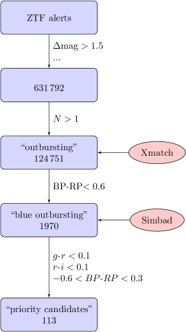
Figure 1: The different steps we used to select candidates. The number in each box shows the unique candidates that passed selection criteria so far. The selection criteria are explained in detail in the text, and a breakdown of the candidates in the last two steps are given in Table 1.

As a first step, we used ZTF to identify outbursting stars. We searched all ZTF alerts (Masci et al., 2019) using a simple set of criteria to identify objects:

• $\mathrm{isdiffpos}=\mathrm{True}$: only positive alerts.

• $\mathrm{distnr}<1.5$; alerts close to a star in the ZTF reference image.

• $\mathrm{psdistnr}<3.0$; alerts close to a star in PS1.

• $(\mathrm{magpsf}-\mathrm{magnr})<-2.5\log_{10}(10^{0.4\times 1.5}-1)$; select stars that become brighter by 1.5 mag or more.

• $\mathrm{braai}>0.9$ or $\mathrm{drb}>0.9$; reject bogus subtractions (Duev et al., 2019).

• NOT $\mathrm{ssdistnr}>12$ & $\mathrm{ssmagnr}<20$; used to remove known, bright asteroids.

• $\mathrm{magnr}>16$; removes bright stars.

With these criteria, we selected 631 792 unique objects.

After inspection of the candidates, we noticed that many objects with only a single alert, possibly bogus subtractions or asteroids that moved within 1” of a star. We, therefore, removed any object for which only one alert passed the previous criteria:

• $N>1$

after this step, 124 751 “outbursting” objects remain.

2.2 Crossmatch with Gaia and Pan-STARRS

For the next step, we queried Vizier for both Gaia and PS1 data using Xmatch. Initially, we used Gaia DR2, but switched to Gaia eDR3 (Brown et al., 2020b) when that became available. We only kept sources with:

• Gaia match within 3″

• $BP-RP<0.6$

These steps reduced the number of candidates to 1970.

2.3 Identification of known sources

We listed all sources with their statistics that passed these criteria. We checked the literature on known AM CVn systems and identified 20 candidates as known AM CVn systems. To better understand where AM CVn systems are located in color space, we added all published AM CVn binaries to the list (Ramsay et al., 2018; Green et al., 2020; van Roestel, 2021; Isogai et al., 2021), including 57 systems that did not appear in our alert query (they are not included in the numbers given in Fig. 1 and Table 1). For the remaining candidates, we used Simbad to determine if a candidate was already identified as a hydrogen-rich CV. We searched for either an identification spectrum, a period from eclipses (Hardy et al., 2017), or a period from superhumps (Kato et al., 2017; Patterson et al., 2005), and marked these systems (199) as ‘not-AM CVn’s and do not consider these any further. An overview of these sources in magnitude and color space is given in Fig. 2.

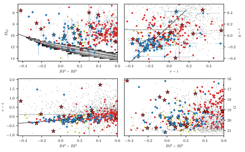
Figure 2: An overview of all blue outbursting sources found using our query. Blue markers show AM CVn and He-CV systems, red show other classified systems, yellow points show unidentified sources that passed all these criteria, the ‘priority candidates’, grey points show other unclassified objects. The grey background in the topleft panel shows the population of nearby white dwarfs. Stars indicate ones for which we obtained an identification spectrum, see Table 2. Dashed lines show the ‘strict’ selection criteria we used to prioritize targets for followup. The black lines show model colors of a DB white dwarf ($\log(g)=8$) (Bergeron et al., 2011).

2.4 Selection of priority candidates

During the course of this work, Gaia eDR3 was released which includes more data and uses improved filter response curves. This changed the $BP$-$RP$ values for some objects, in some cases by as much as 0.6 mag, and changed the color of the false positives for which we already obtained spectra to much redder values.

The updated Gaia colors and an evaluation of the objects observed so far prompted us to use stricter color selection criteria. Inspection of the Pan-STARRS colors showed that many known AM CVn systems have blue colors in $g$-$r$ and $r$-$i$, while false positives are red in one or both of these colors (see Fig. 2). We, therefore, used the empirically chosen (but see Carter et al., 2013b) stricter set of criteria to identify high priority candidates:

• $-0.6<BP$-$RP<0.3$

• $g$-$r<0.1$

• $r$-$i<0.1$

Table 1 summarises the properties of the selected candidates. This shows that the strict selection criteria reduce the number of candidates by an order of magnitude, but also excludes half of the known AM CVn systems. Based on the ratio of known AM CVn systems versus other systems, $\mathord{\sim}$20% of the objects that passed the strict criteria are AM CVn systems. With 59 unidentified systems that pass the strict criteria, we can expect to find $\mathord{\sim}15$ new AM CVn systems by obtaining identification spectra of this sample.

Table 1: The details of the candidates selected using the initial selection criteria and the strict criteria. The ‘AM CVn’ column shows the number of known AM CVn systems, the ‘H-CV’ column shows the number of known hydrogen CV, the ‘unknown’ column lists the number of unclassified objects. The rows indicate if Gaia measured a parallax regardless of uncertainty.

All candidates
	AM CVn	other CV	unknown	total
Gaia plx.	18	185	727	930
no plx.	2	14	1024	1040
total	20	199	1751	1970
Strict selection
	AM CVn	other CV	unknown	total
Gaia plx.	9	39	24	72
no plx.	1	5	35	41
total	10	44	59	113

3 Followup observations

3.1 Spectroscopic followup

We used the 4.2m William Herschel Telescope (La Palma, Sp) in June 2019 to observe 7 candidates with ACAM (Benn et al., 2008). ACAM has a resolution of $R\approx 400$ and wavelength coverage of 4000–9000Å. We used exposure times of 900-1200 seconds. The spectra were reduced using the ACAM quick reduction pipeline.

We obtained 20 identification spectra with the 10m Keck I Telescope (HI, USA) and the Low Resolution Imaging Spectrometer (LRIS; Oke et al. 1995; McCarthy et al. 1998). Either the R600 grism for the blue arm ($R\approx 1100$) and the R600 grating for the red arm ($R\approx 1400$), or the R400 grism for the blue arm ($R\approx 600$) and R600 grating for the red arm ($R\approx 1000$) were used. The wavelength range is approximately 3200–8000/10000Å.

For two objects, we obtained spectra with DEIMOS (Faber et al., 2003) mounted on the 10m Keck II telescope. One spectrum was obtained with the 600ZD grating ($R\approx 1400$), the second with the 1200B grating ($R\approx 4500$). Data were reduced with the standard pipeline.

We obtained spectra of 6 objects with the two-arm Kast spectrograph mounted at the 3-m Shane telescope (Miller & Stone, 1994). In the blue and red arm, we used the 600/4310 and 600/5000 gratings. Combined with the 2″ slit, the resolution is R$\approx$2200 and R$\approx$2500. We used exposure times between 1500 and 3600 seconds, depending on target brightness. We split the exposures in the red arm to mitigate the effects of cosmic rays. The data were reduced using a PipeIt based pipeline (Prochaska et al., 2020).

3.2 CHIMERA fast cadence photometry

We obtained $g$ and $r$ lightcurves of ZTF18acnnabo, ZTF18acujsfl, and ZTF19abdsnjm. We used CHIMERA (Harding et al., 2016), a dual-channel photometer mounted on the Hale 200-inch (5.1 m) Telescope at Palomar Observatory (CA, USA). Each of the images was bias subtracted and divided by twilight flat fields.

The ULTRACAM pipeline was utilized to obtain aperture photometry using a 1.5 FWHM-sized aperture (see Dhillon et al., 2007). A differential lightcurve was created by simply dividing the counts of the target by the counts from the reference star. Images were timestamped using a GPS receiver.

4 Individual systems

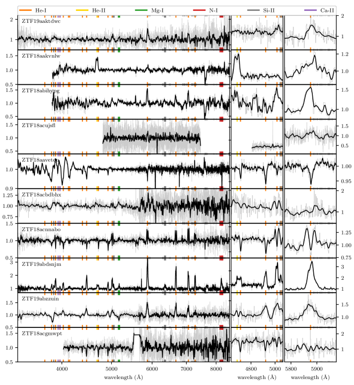
Figure 3: The spectra of the 10 systems which do not show any hydrogen in their spectra. The left panels show the entire spectrum and the two panels on the right zoom in on He spectral lines. The thin gray lines are original spectra and the thick black lines show spectra convolved with a Gaussian kernel for visibility. Vertical colored lines show the rest wavelength of different elements.

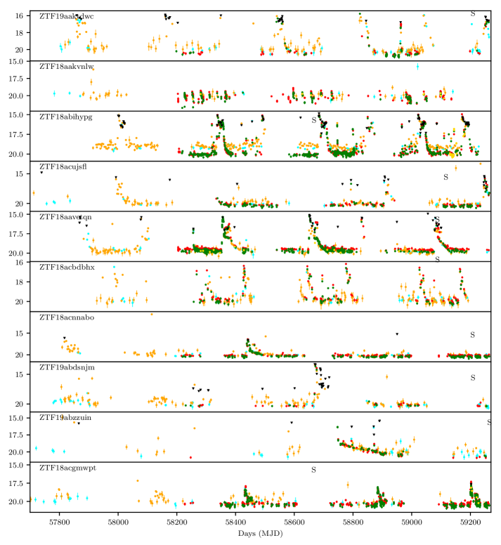
Figure 4: The lightcurves of the 10 systems which do not show any hydrogen in their spectra. We show ZTF forced photometry ($g$, $r$, and $i$ in green, red, and gold), ATLAS data ($c$ and $o$ in cyan and orange), and ASASSN data in black. An ’S’ indicates when the spectrum was obtained.

We obtained spectra of 35 objects of which 25 show hydrogen lines, shown in the Appendix. Most spectra are typical for hydrogen-rich CVs with strong Balmer emission lines. A notable exception is the spectrum of ZTF19aadtlkv which shows a broad emission line, possibly cyclotron emission of a CV with a large magnetic field (e.g Szkody et al., 2003, 2020). The remaining 10 objects, shown in Fig. 3, do not show hydrogen in their spectra. We discuss each of these objects individually in this section.

To characterize these objects, we obtained archival photometry for these sources, shown in Fig. 4. The figure shows ZTF forced photometry (Masci et al., 2019), ATLAS forced photometry (Tonry et al., 2018; Smith et al., 2020), and ASAS-SN (Shappee et al., 2014; Kochanek et al., 2017) data for each object.

Similar to SU UMa-type cataclysmic variables, AM CVn systems show normal outbursts and also super-outbursts (Warner, 1995). Super-outbursts last a few weeks and are 2–5 magnitudes in amplitude, while normal outbursts are much shorter, typically less than one night and are lower in amplitude. Levitan et al. (2015) and Cannizzo & Ramsay (2019) showed that the outburst frequency, amplitude, and superoutburst duration correlate with the orbital period of the AM CVn systems. We do note that the recent discovery of a very long outburst with a rather small amplitude of a long period AM CVn system complicates this simple picture (Rivera Sandoval et al., 2020).

To estimate the orbital period we use the superoutburst recurrence time because the large amount of data available makes this easy and the correlation is the strongest. We visually inspected and marked the superoutburst peak times. We calculated the approximate large common divisor of the time differences. If there were multiple solutions, we inspected the lightcurve to determine which solution was best.

We convert the recurrence time to an orbital period using:

$$P_{\mathrm{orb}}(\mathrm{min})=29.59\left(\frac{\tau_{\mathrm{rec}}\mathrm{(}d)-24.7}{100}\right)^{0.136}$$ (1)

which is the equation from Levitan et al. (2015) rearranged. We assume a 5% uncertainty or propagate the estimated variance of the recurrence time, whichever is larger.

4.1 ZTF19aaktdwc

This source was previously discovered by CRTS (CSS130419 J132918-121622, Drake et al. 2014) as an unclassified outbursting star. A spectrum was obtained by Oliveira et al. (2020), but it was completely featureless. The spectrum we obtained shows three weak, but significant, He-I emission line which confirms that this is an AM CVn binary.

The lightcurve shows at least 6 superoutbursts in the last 5 years that lasted a few weeks. There are also a few shorter and lower amplitude outbursts in between. The recurrence time of the superoutbursts is $\sim 210$d and very regular. This corresponds to an orbital period of $\mathord{\sim}32.2$  minutes.

4.2 ZTF18aakvnlw

This source was identified as an outbursting star by CRTS (CRTS J1647+4338) and also included in Szkody et al. (2020). Based on a spectrum which shows strong He-II emission and possibly H$\alpha$, Breedt et al. (2014) speculate that this system is a He-CV (see also Green et al. 2020). We also obtained a spectrum with ACAM, and also see a strong, double-peaked He-II line. A closer inspection of the spectrum suggests some He-I emission, but no sign of any H$\alpha$ emission. As already indicated by Breedt et al. (2014), strong He-II is typically associated with magnetic CVs.

The lightcurve shows frequent, relatively low amplitude variability. The lightcurve does not show obvious superoutbursts and appears different from all other lightcurves. We cannot confidently classify this system as an AM CVn system or not. Phase-resolved spectroscopy is needed to determine the orbital period to definitively classify this object.

4.3 ZTF18abihypg

Szkody et al. (2020) discovered this source as an outbursting star and a CV candidate. Despite being very blue and not passing the ’strict’ criteria, we chose to get a spectrum of this source because the lightcurve showed many regular outbursts after the super-outbursts.

The spectrum shows clear, broad He-I emission lines. There is also a broad line at 8196Å, likely N-I, sometimes seen in other AM CVn systems. Given the spectral features, we classify this source as a new AM CVn binary.

The lightcurve is similar to ZTF19aaktdwc with 6 (maybe 7) superoutbursts in the last 5 years with a recurrence time of $\mathord{\sim}160$d. This corresponds to a period of $\mathord{\sim}31.2$  minutes. The frequency of regular outbursts is high in this system, with a total of 10 of them, typically lasting only a day.

4.4 ZTF18acujsfl

The spectrum is almost featureless but on closer inspection, three low amplitude, broad, and possibly double-peaked He-I emission lines can be seen. The very long outburst recurrence time ($\mathord{\sim}320$ d) and low amplitude of the emission lines suggest that this is a longer period system, $P_{\mathrm{orb}}\mathord{\sim}34.3$ minutes.

The lightcurve shows just 2 (maybe 3) superoutbursts. There are possibly three regular outbursts, but these are not well sampled. We estimate the recurrence time to be $\mathord{\sim}310$ d based on the interval between the last two observed outbursts. This time corresponds to an orbital period of $\sim 34.1$  minutes. We obtained a 75-minute long lightcurve in $g$ and $r$ at a cadence of 5 seconds with CHIMERA. Both the $g$ and $r$ lightcurve did not show any sign of variability.

4.5 ZTF18aavetqn

This system was discovered by MASTER (Balanutsa et al., 2014), detected by Gaiaas Gaia18cjw, and was reported as a CV-candidate by Szkody et al. (2020). It is located in the Kepler field (KIC 8683556). The spectrum was obtained during the latest superoutburst and shows helium absorption lines, which are especially strong at the blue end of the spectrum. This is consistent with AM CVn systems in outburst.

The lightcurve shows 5 superoutbursts with 1 (maybe 3) normal outbursts. The time between superoutbursts is irregular, ranging from 170 to 290 days, with a best estimate of 230 days. This corresponds to a period of 32.6 (31.7–33.8) minutes. Kato et al. (2017) reports a superhump period of $31.8$ m which corresponds to an orbital period of $31.5$ m (if we assume the same period excess of 0.8% as was found for YZ LMi Copperwheat et al. 2011). This is in good agreement with the estimated orbital period based on the superoutburst recurrence time.

4.6 ZTF18acbdbhx

Drake et al. (2014) reported this as an outbursting star based on the CRTS data. The spectrum shows weak He-I emission lines. There seems to be a double-peaked line at He-I 5015Å, and we, therefore, classify this as an AM CVn system.

The lightcurve shows 5–7 superoutbursts, with about 9 normal outbursts. The superoutburst recurrence time is regular at 130 days, which corresponds to a period of $29.4$ m.

4.7 ZTF18acnnabo

This system was identified as an outbursting source by MASTER (Shumkov et al., 2013). The spectrum shows very clear double-peaked He-I emission lines in the red part of the spectrum. The He-I lines at the blue end of the spectrum appear as absorption lines. In addition, Ca-I H&K lines are clearly visible in absorption. The very pronounced double-peaked structure of the He lines indicates that the inclination is high. This means that the system could potentially show eclipses. We obtained a 75-minute long lightcurve in $g$ and $r$ at a cadence of 5 seconds but there was no evidence of eclipses.

The lightcurve shows only two long outbursts, lasting at least 50 days followed by three normal outbursts. The outburst recurrence time is either 335 or 670 days. We used the MASTER detection and a PTF detection confirming the 670 day recurrence time. This puts the orbital period at $38.2$ m.

4.8 ZTF19abdsnjm

This source is also known as ASASSN-19rg and Gaia19dlb. The spectrum is the most feature-rich of the entire sample. It shows very strong double-peaked He-I emission lines spanning the entire spectral range, as well as He-II-4686Å. The spectrum also shows a Mg-I emission line at 5167/72/83Å, and likely Si-II emission lines at 3856, 5175, 6347/71Å. There is also a broad emission line at 8196Å, likely N-I emission.

The lightcurve shows only one superoutburst, with 5 shorter outbursts in the last 5 years. CRTS reports three detections on the night of MJD=56030, which puts an upper limit to the recurrence time to 7 years, corresponding to a period of 45 m.

Josch H. and B. Monard observed the system while it was in outburst and found a superhump period of $43.8$ m, consistent with our estimate. We obtained a 60-minute long lightcurve in $g$ and $r$ at a cadence of 5 seconds while the system was in quiescence. The system showed no sign of variability in the lightcurve.

4.9 ZTF19abzzuin

The spectrum shows He-I emission lines. The He-I lines at longer wavelengths show double-peaked profiles. The spectrum also shows a Mg-I absorption line at 5167/72/83 Å and Mg-II absorption line at 3832/38 Å.

The lightcurve shows only the tail end of one long superoutburst. The first detections could show the actual outburst, but the decay is fast enough to be a normal outburst similar to one seen later during the decay. The duration of the outburst and long recurrence time suggests a period $\gtrsim 40$–$50$ m.

4.10 ZTF18acgmwpt

This source has been detected by Gaia as Gaia18djd. Because the SNR is low, the spectrum does not show any obvious features. A closer inspection shows He-I absorption lines on the blue side. The SNR is too low in the red to discern any features. We do classify this system as an AM CVn because of the detection of He-I lines.

The lightcurve shows three clear and two likely superoutbursts with a relatively low amplitude of 2 magnitudes. In the tail of each outburst, there are signs of normal outbursts. The outburst recurrence time is either 155 or 332 days, corresponding to orbital periods of $30.7$ or $34.5$ minutes.

5 Results

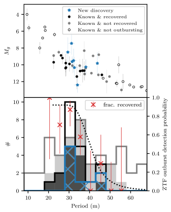
Figure 5: The top panel shows the absolute magnitude versus the orbital period for AM CVn for which both parameters are known. Blue stars indicate the new discoveries, black dots show outbursting systems we recovered, grey dots show outbursting systems we have not recovered, and open circles show non-outbursting systems. The bottom panel shows the period distribution of all AM CVn systems with known periods. New discoveries are indicated with the hashed blue histogram, the grey histogram shows the known outbursting AM CVn systems. The recovered systems are shown in darker grey. The grey line shows all previously known AM CVn systems, including systems that do not show alerts. The thick black line shows all AM CVn systems recovered in our search. Red crosses show the recovery fraction of known systems and the dashed line shows the estimated probability that ZTF could have observed at least one outburst.

5.1 Selection of AM CVn candidates

We identified 1970 blue, outbursting sources using ZTF, Gaia, and Pan-STARRS, of which 1751 are not classified. Based on colors of known AM CVn and other outbursting systems, we defined a simple and strict set of criteria designed to optimize the AM CVn discovery rate. A total of 113 sources pass the strict criteria, of which 59 are unclassified. We obtained 35 identification spectra in total, 18 of which are part of the set of strong AM CVn candidates. Analysis of the spectra shows that 19 systems show some kind of hydrogen emission and are typical cataclysmic variables. Out of the 10 sources which do not show hydrogen, 9 sources are new AM CVn systems, (of which 8 passed the strict criteria), and one source for which the classification is uncertain.

5.2 Characterization of 9 new AM CVn systems

The 9 new AM CVn systems are typical for outbursting AM CVn systems (Duffy et al., 2021).and show both outbursts and super-outbursts. In some cases, there are hints of ‘dips’ a few days after the peak of a super-outburst. In addition, normal outbursts typically last less than one night and tend to be more frequent after a super-outburst. We predict the orbital periods from the outburst recurrence time. The orbital periods are in the range of 29 to 34 minutes, with one system with a period estimated to be between 40–50 minutes. The distribution of periods shown in Fig. 5.

Spectroscopically the 9 new systems are diverse: some systems show strong emission lines, some show very weak emission lines, and other systems show absorption lines. Among the emission lines, some are double-peaked, while others show a single emission line. This diversity is also seen in known AM CVn systems and can be explained by differences in accretion state and inclination. A few systems, most notably ZTF18abdsnjm, also show metal lines including Ca, Mg, Si, and possibly N, also seen in other AM CVn systems (Nelemans et al., 2004).

6 Discussion

The goal of this work is to determine if and how efficiently AM CVn systems can be identified by combining ZTF-alerts and color information. Here, we briefly discuss the completeness, efficiency, biases, and limitations of this method.

6.1 Selection by outbursts

The completeness of our method to find all AM CVn systems is limited by our search to objects which show outbursts of 1.5 magnitudes or more. While this selection method reduces the number of candidates by 4 orders of magnitude (Fig. 1), it does mean that we will only find AM CVn systems that outburst; in the period range of $22\lesssim P_{\mathrm{orb}}\lesssim 50$ m. To find the shorter and longer period AM CVn systems that do not show outbursts, other methods are needed (e.g. Burdge et al., 2020; van Roestel, 2021).

Superoutburst amplitudes of AM CVn systems typically range from $2$–$5$ magnitudes (Levitan et al., 2015), which is larger than the 1.5 magnitude limit we chose. This means that the recovery efficiency of outbursting AM CVn systems is only limited by the ZTF coverage, sampling frequency, and time baseline. To better understand these aspects, we compare our sample with the known sample of AM CVn systems, as shown in Fig. 5. Using the already known systems, we calculate the recovery efficiency. We recovered most of the systems with periods between $22\lesssim P\lesssim 40$ min. The objects we did not recover in this period range were either at low declinations or were too bright (these were excluded from the recovery fraction efficiency). At periods of $P\gtrsim 40$ min, the recovery efficiency decreases sharply. Inspection of the lightcurves shows that these objects did not outburst when ZTF was watching.

6.2 Selection by outbursts and colors

As can be seen in Fig. 2, AM CVn systems are typically bluer compared to the overall population of outbursting CVs. Of the known AM CVn systems, 61 out of 67 (91%) pass the first color cut ($BP$-$RP<0.6$), while reducing the number of candidates by 3 orders of magnitudes. Based on the known systems that pass this cut, we can expect $\mathord{\sim}9\%$ of the objects to be an AM CVn system (based on the known systems, see Table 1). As explained in Section 2, this sample is still too large to followup with long-slit spectroscopy and we use a second more strict color cut to prioritize targets. From the known systems, we estimated a $\mathord{\sim}$20% (10/54) AM CVn-rate of the ‘strict’ candidates (Section 2). As shown in Table 2, 8 out of 18 observed ‘strict’ candidates are AM CVn systems (44%). We did focus on the blue-est systems and systems with a parallax measurement. In addition, we also used the known superhump periods of two targets to prioritise them for followup. If we exclude these two systems, we still reach an efficiency of 38%.

The ‘strict’ criteria were chosen to increase the true positive rate, however, the trade-off is low completeness. The ’strict’ criteria reduce the number of known, outbursting AM CVn systems by half (Table 1). Isolated white dwarfs hotter than 8000 K, (less than the coolest white dwarf in an AM CVn system) should pass the strict criteria (e.g. Bergeron et al., 2011). However, an inspection of AM CVn color versus orbital period shows that there are many redder systems in the $BP$-$RP$, $g$-$r$, and $r$-$i$ colors in the range of 22-30 minutes. If we apply the ‘strict’ criteria, we notice that almost all systems in the 22-30 minutes do not pass these criteria. By focusing the followup spectroscopy on the bluest sources, we have biased ourselves against systems with periods shorter than $\mathord{\sim}30$ minutes.

This can be explained by the more frequent outbursts for short period systems. Outbursts can ‘scramble’ color measurements, especially for non-simultaneous observations like Pan-STARRS. If the object is observed in outburst in one band and in quiescence in the other, the magnitude difference does not represent the color of the system (e.g. the lower-left panel of Fig. 2). This is, again, especially relevant for short-period systems that show frequent outbursts.

6.3 Improvements

Overall, the method we use is straightforward and simple and both the efficiency and completeness can be improved in a number of ways. First, we can expand the selection of outbursting sources by using CRTS (Breedt et al., 2012; Drake et al., 2014), PTF (Law et al., 2009; Rau et al., 2009), and Gaia alerts (e.g. Campbell et al., 2015). The longer time-baseline of these surveys should improve the detection efficiency in the period range of long period systems; $40\lesssim P_{\mathrm{orb}}\lesssim 50$ m. We also note that most of the known AM CVn systems are in the Northern hemisphere which suggests that there are many undiscovered AM CVn systems in the Southern hemisphere. For example, Gaia alerts (Campbell et al., 2015) combined with the Gaia quiescence colors can be used to find them.

Second, as noted in the discussion, using average (Pan-STARRS) colors can be scrambled by outbursts which can cause false-negatives. To resolve this, we can use the ZTF, ATLAS, and Pan-STARRS multi-color lightcurves to measure the color only when the system is in quiescence. This would alleviate the problem that outbursts introduce noise in the color measurements and solve the bias against frequently outbursting, short-period systems.

In addition, we have not used the temporal information from the lightcurves to attempt to identify AM CVn candidates. For example, AM CVn systems tend to show many normal outbursts after a superoutburst, which is only rarely seen in hydrogen-rich CVs. The amplitude, duration, and recurrence time of superoutbursts are also characteristic and could be used to distinguish AM CVn systems from hydrogen-rich CVs. In addition, if the sampling is very high, a measurement of a superhump period could be used to identify AM CVn systems.

Based on the true positive rate and number of candidates, we estimate that there are another 20-30 outbursting AM CVn systems to be found with a Gaia parallax measurement in the ZTF footprint. We speculate that a similar number can be found in the Southern hemisphere which is relatively unexplored, which means that there is the potential to double the known number of AM CVn systems.

7 Conclusions

We have described a spectroscopic survey aimed at finding new AM CVn systems by focusing on blue, outbursting sources identified by ZTF. We specified a set of strict criteria based on Pan-STARRS and Gaia colors. 103 candidates pass these criteria and based on the number of known sources, we estimated that $25\%$ of them are AM CVn systems. A detailed analysis showed that focusing on the bluest sources increased the purity of the sample, but also produced a bias against discovering short-period AM CVn systems.

We obtained spectra of 35 candidates (18 from the strict selection) and identified 9 new AM CVn systems. All spectra show helium lines, either in emission or absorption. A few systems also show metal absorption lines. From the recurrence frequency of super-outbursts, we estimate that their orbital periods range from 28 to 40 minutes. We encourage observers to obtain high cadence photometry when these systems outburst to confirm the orbital periods.

For future work, we will obtain identification for all unidentified objects that pass the strict criteria. We will aim to improve completeness and efficiency by including data from other surveys, e.g. CRTS (Drake et al., 2014), Gaia-alerts (Wyrzykowski et al., 2012), ATLAS (Tonry et al., 2018), Skymapper (Wolf et al., 2018), BlackGEM (Groot, 2019). Finally, we will explore methods that use the multi-color lightcurves directly to improve the identification of candidates. The goal is to find all AM CVn systems with Gaia parallax measurements with the goal to study the population properties (space density, Galactic distribution, period distribution etc.) but also to find rare AM CVn systems; eclipsing systems, systems with large magnetic fields, or systems with unusual chemical abundances.

In addition, developing efficient selection methods will also be important for VRO which will obtain 5-band lightcurves and find many faint candidates for which followup spectroscopy will be expensive.

Table 2: An overview of all objects for which we obtained a spectrum. The column ’strict’ indicates if the sources passed the strict color selection, see section 2. Distances are taken from Bailer-Jones et al. (2021).

ZTF ID	RA	Dec	$G$	$BP$-$RP$	dist. (pc)	spectrum	date	Strict	AM CVn	Notes
ZTF17aacmiwg	10 53 33.8	28 50 35.5	19.18	0.42	$1890^{+700}_{-650}$	ACAM	2019-06-25	✗	✗	$H\alpha$ emission, Balmer and He-I absorption
ZTF18aabxxwr	13 15 14.4	42 47 46.9	19.92	0.69	$1590^{+410}_{-290}$	ACAM	2019-06-25	✗	✗	strong Balmer and He-I emission
ZTF19aaktdwc	13 29 18.5	-12 16 22.3	20.37	0.14	$1960^{+1250}_{-1320}$	ACAM	2019-06-25	✓	✓	no Balmer lines, He-I emission, maybe He-II emission
ZTF19aadtlkv	13 48 01.9	-09 17 41.7	20.73	-0.11		ACAM	2019-06-25	✗	✗	strong Balmer emission, broad synchrotron beaming at 5543Å
ZTF18aakvnlw	16 47 48.0	43 38 45.0	20.01	-0.25	$2480^{+860}_{-850}$	ACAM	2019-06-25	✗	?	strong He-II emission, He-CV (Green et al., 2020)
ZTF18abcxayn	19 19 15.7	35 08 50.3	18.96	0.33	$1960^{+980}_{-410}$	ACAM	2019-06-25	✗	✗	$H\alpha$ emission, Balmer and He-I absorption
ZTF18abihypg	21 28 22.1	63 25 57.3	19.99	0.31	$780^{+190}_{-100}$	ACAM	2019-06-25	✗	✓	HeI emission
ZTF18abwjzpq	02 24 36.4	37 20 21.4	20.63	0.21	$860^{+440}_{-300}$	DEIMOS	2020-09-21	✓	✗	strong double peaked $H\alpha$, weak double peaked Balmer and He-I
ZTF18acujsfl	04 49 30.1	02 51 53.7	20.30	0.08	$1170^{+490}_{-450}$	DEIMOS	2020-09-21	✓	✓	double peaked He-I
ZTF18aavetqn	19 18 42.0	44 49 12.3	19.54	-0.07	$1020^{+320}_{-160}$	LRIS	2020-08-19	✓	✓	Mg-II
ZTF18abobpds	20 15 35.3	-14 16 44.4	20.49	0.32		LRIS	2020-08-19	✗	✗	strong Balmer, weak He-I emission
ZTF19aavhqxe	20 42 58.8	-00 33 54.0	17.29	0.00		LRIS	2020-08-19	✗	✗	moderate Balmer emission, weak He-I
ZTF18acbdbhx	21 08 20.6	-13 49 09.3	19.71	0.12	$1560^{+850}_{-430}$	LRIS	2020-08-19	✓	✓	almost featureless, shows very weak weak He-I
ZTF18abhqcfi	00 13 01.1	51 13 58.8	20.12	0.69		LRIS	2020-12-17	✗	✗	strong Balmer, weak He-I emission
ZTF18abtnfzy	06 26 09.6	67 45 31.3	20.18	0.64	$1690^{+710}_{-490}$	LRIS	2020-12-17	✗	✗	strong Balmer, weak He-I emission
ZTF18acnnabo	08 20 47.6	68 04 24.0	20.19	0.03	$2450^{+1460}_{-830}$	LRIS	2020-12-17	✓	✓	double peaked He-I
ZTF19aazgilw	10 44 50.1	23 24 30.9	19.83	0.20	$420^{+150}_{-70}$	LRIS	2020-12-17	✓	✗	Balmer emission and broad absorption, weak He-I emission
ZTF18aabxycb	13 15 14.4	42 47 44.6	19.92	0.69	$1590^{+410}_{-290}$	LRIS	2020-12-17	✗	✗	strong Balmer emission, weak He-I
ZTF19abdsnjm	13 25 58.1	-14 52 26.0	20.38	0.04	$1160^{+520}_{-370}$	LRIS	2020-12-17	✓	✓	He-I/II, MgII, SiII, and NI emission
ZTF19aamfvdm	05 53 15.7	-26 48 46.9	20.32	0.21	$1000^{+780}_{-310}$	LRIS	2021-02-12	✓	✗	strong Balmer emission, He-I emission
ZTF19aadqrmz	07 07 08.0	-00 56 41.1	20.42	0.18	$2160^{+2090}_{-1040}$	LRIS	2021-02-12	✓	✗	strong Balmer, weak He-I emission
ZTF19abzzuin	08 44 19.7	06 39 50.2	21.16	-0.02		LRIS	2021-02-12	✓	✓	He-I emission, MgII absorption
ZTF18aczeouv	11 38 35.6	04 44 54.8	19.13	0.58	$520^{+150}_{-90}$	LRIS	2021-02-12	✗	✗	double peaked Balmer and strong, narrow absorption in H and He-I
ZTF18acgmwpt	07 01 15.8	50 23 21.5	20.50	0.14	$1640^{+1290}_{-670}$	LRIS	2021-02-15	✓	✓	Mg-II
ZTF18aaacggd	07 44 00.5	41 55 03.5	20.64	0.09	$610^{+300}_{-230}$	LRIS	2021-02-15	✓	✗	double peaked $H\alpha$, weak $H\beta$
ZTF18achzexf	08 29 25.3	-00 13 47.5	16.20	-0.42	$1370^{+170}_{-150}$	LRIS	2021-02-15	✗	✗	strong Balmer and Paschen emission, weak He-I emission
ZTF18aawqkva	15 44 28.1	33 57 24.3	18.06	-0.03		LRIS	2021-02-15	✓	✗	outburst spectrum. Weak $H\alpha$ emission, Balmer and He-I absorption
ZTF18abtugvf	18 26 34.7	22 56 10.5	20.74	-0.21		LRIS	2021-02-15	✗	✗	Balmer emission
ZTF18aavoyoq	18 14 39.7	50 18 34.9	17.76	-0.08		LRIS	2021-02-15	✓	✗	broad Balmer emission
ZTF18abcxayn	19 19 15.7	35 08 50.1	18.96	0.33	$1960^{+990}_{-400}$	Kast	2021-04-13	✗	?	low SNR, no obvious lines
ZTF18abmouep	16 36 18.3	-01 15 06.2	19.20	0.40	$5060^{+3120}_{-1660}$	Kast	2021-04-18	✗	✗	H$\alpha$ emission
ZTF18acecect	07 28 42.8	53 37 39.3	17.44	0.30	$2470^{+870}_{-400}$	Kast	2021-04-29	✓	✗	Balmer emission lines
ZTF19aahvgyg	09 08 52.2	07 16 39.3	19.77	0.03	$1920^{+1030}_{-740}$	Kast	2021-04-29	✓	✗?	low SNR, maybe Balmer emission
ZTF19acecitx	06 21 50.3	-24 43 47.2	19.47	-0.25	$3460^{+3000}_{-1460}$	Kast	2021-04-29	✓	?	low SNR
ZTF21aapvkyy	19 17 08.3	30 00 24.56	20.92	0.64	$3040^{+1170}_{-1300}$	Kast	2021-04-29	✗	✗	strong H$\alpha$ emission, He-I emission

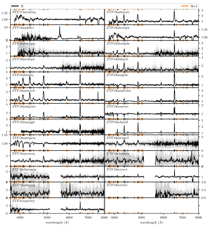
Figure 6: The spectra of that show hydrogen lines. The grey spectra show the original spectra and the black line show the spectra convolved with a Gaussian kernel for visibility. Vertical colored lines show the wavelengths of H and He lines.

References

- Astropy Collaboration et al. (2013) Astropy Collaboration, Robitaille, T. P., Tollerud, E. J., et al. 2013, Astronomy and Astrophysics, 558, A33, doi: 10.1051/0004-6361/201322068
- Astropy Collaboration et al. (2018) Astropy Collaboration, Price-Whelan, A. M., Sipőcz, B. M., et al. 2018, The Astronomical Journal, 156, 123, doi: 10.3847/1538-3881/aabc4f
- Bailer-Jones et al. (2021) Bailer-Jones, C. A. L., Rybizki, J., Fouesneau, M., Demleitner, M., & Andrae, R. 2021, The Astronomical Journal, 161, 147, doi: 10.3847/1538-3881/abd806
- Balanutsa et al. (2014) Balanutsa, P., Denisenko, D., Lipunov, V., et al. 2014, The Astronomer’s Telegram, 6071. http://adsabs.harvard.edu/abs/2014ATel.6071....1B
- Bellm et al. (2019) Bellm, E., Kulkarni, S., & Graham, M. 2019, 233, 363.08. http://adsabs.harvard.edu/abs/2019AAS...23336308B
- Benn et al. (2008) Benn, C., Dee, K., & Agócs, T. 2008, in Ground-based and airborne instrumentation for astronomy II, ed. I. S. McLean & M. M. Casali, Vol. 7014 (SPIE), 2384 – 2395, doi: 10.1117/12.788694
- Bergeron et al. (2011) Bergeron, P., Wesemael, F., Dufour, P., et al. 2011, The Astrophysical Journal, 737, 28, doi: 10.1088/0004-637X/737/1/28
- Bildsten et al. (2007) Bildsten, L., Shen, K. J., Weinberg, N. N., & Nelemans, G. 2007, The Astrophysical Journal Letters, 662, L95, doi: 10.1086/519489
- Bildsten et al. (2006) Bildsten, L., Townsley, D. M., Deloye, C. J., & Nelemans, G. 2006, The Astrophysical Journal, 640, 466, doi: 10.1086/500080
- Breedt et al. (2012) Breedt, E., Gänsicke, B. T., Marsh, T. R., et al. 2012, Monthly Notices of the Royal Astronomical Society, 425, 2548, doi: 10.1111/j.1365-2966.2012.21724.x
- Breedt et al. (2014) Breedt, E., Gänsicke, B. T., Drake, A. J., et al. 2014, Monthly Notices of the Royal Astronomical Society, 443, 3174, doi: 10.1093/mnras/stu1377
- Breivik et al. (2018) Breivik, K., Kremer, K., Bueno, M., et al. 2018, The Astrophysical Journal Letters, 854, L1, doi: 10.3847/2041-8213/aaaa23
- Brown et al. (2020a) Brown, A. G. A., Vallenari, A., Prusti, T., & Bruijne, J. H. J. d. 2020a, Astronomy & Astrophysics, doi: 10.1051/0004-6361/202039657
- Brown et al. (2020b) —. 2020b, Astronomy & Astrophysics, doi: 10.1051/0004-6361/202039657
- Burdge et al. (2020) Burdge, K. B., Prince, T. A., Fuller, J., et al. 2020, The Astrophysical Journal, 905, 32, doi: 10.3847/1538-4357/abc261
- Campbell et al. (2015) Campbell, H. C., Marsh, T. R., Fraser, M., et al. 2015, Monthly Notices of the Royal Astronomical Society, 452, 1060, doi: 10.1093/mnras/stv1224
- Cannizzo & Nelemans (2015) Cannizzo, J. K., & Nelemans, G. 2015, The Astrophysical Journal, 803, 19, doi: 10.1088/0004-637X/803/1/19
- Cannizzo & Ramsay (2019) Cannizzo, J. K., & Ramsay, G. 2019, The Astronomical Journal, 157, 130, doi: 10.3847/1538-3881/ab04ac
- Carter et al. (2014a) Carter, P. J., Steeghs, D., Marsh, T. R., et al. 2014a, MNRAS, 437, 2894, doi: 10.1093/mnras/stt2103
- Carter et al. (2013a) Carter, P. J., Steeghs, D., de Miguel, E., et al. 2013a, Monthly Notices of the Royal Astronomical Society, 431, 372, doi: 10.1093/mnras/stt169
- Carter et al. (2013b) Carter, P. J., Marsh, T. R., Steeghs, D., et al. 2013b, Monthly Notices of the Royal Astronomical Society, 429, 2143, doi: 10.1093/mnras/sts485
- Carter et al. (2014b) Carter, P. J., Gänsicke, B. T., Steeghs, D., et al. 2014b, MNRAS, 439, 2848, doi: 10.1093/mnras/stu142
- Carter et al. (2014) Carter, P. J., Gänsicke, B. T., Steeghs, D., et al. 2014, Monthly Notices of the Royal Astronomical Society, 439, 2848, doi: 10.1093/mnras/stu142
- Chambers et al. (2016) Chambers, K. C., Magnier, E. A., Metcalfe, N., et al. 2016, arXiv e-prints, arXiv:1612.05560
- Coleman et al. (2018) Coleman, M. S. B., Blaes, O., Hirose, S., & Hauschildt, P. H. 2018, The Astrophysical Journal, 857, 52, doi: 10.3847/1538-4357/aab6a7
- Copperwheat et al. (2011) Copperwheat, C. M., Marsh, T. R., Littlefair, S. P., et al. 2011, Monthly Notices of the Royal Astronomical Society, 410, 1113, doi: 10.1111/j.1365-2966.2010.17508.x
- Dhillon et al. (2007) Dhillon, V. S., Marsh, T. R., Stevenson, M. J., et al. 2007, Monthly Notices of the Royal Astronomical Society, 378, 825, doi: 10.1111/j.1365-2966.2007.11881.x
- Drake et al. (2014) Drake, A. J., Graham, M. J., Djorgovski, S. G., et al. 2014, The Astrophysical Journal Supplement Series, 213, 9, doi: 10.1088/0067-0049/213/1/9
- Duev et al. (2019) Duev, D. A., Mahabal, A., Masci, F. J., et al. 2019, Monthly Notices of the Royal Astronomical Society, stz2357, doi: 10.1093/mnras/stz2357
- Duffy et al. (2021) Duffy, C., Ramsay, G., Steeghs, D., et al. 2021, arXiv e-prints, 2102, arXiv:2102.04428. http://adsabs.harvard.edu/abs/2021arXiv210204428D
- Faber et al. (2003) Faber, S. M., Phillips, A. C., Kibrick, R. I., et al. 2003, 4841, 1657, doi: 10.1117/12.460346
- Ginsburg et al. (2019) Ginsburg, A., Sipőcz, B. M., Brasseur, C. E., et al. 2019, The Astronomical Journal, 157, 98, doi: 10.3847/1538-3881/aafc33
- Graham et al. (2019) Graham, M. J., Kulkarni, S. R., Bellm, E. C., et al. 2019, 131, 078001, doi: 10.1088/1538-3873/ab006c
- Green et al. (2018a) Green, M. J., Marsh, T. R., Steeghs, D. T. H., et al. 2018a, Monthly Notices of the Royal Astronomical Society, 476, 1663, doi: 10.1093/mnras/sty299
- Green et al. (2018b) Green, M. J., Hermes, J. J., Marsh, T. R., et al. 2018b, Monthly Notices of the Royal Astronomical Society, 477, 5646, doi: 10.1093/mnras/sty1032
- Green et al. (2020) Green, M. J., Marsh, T. R., Carter, P. J., et al. 2020, Monthly Notices of the Royal Astronomical Society, 496, 1243, doi: 10.1093/mnras/staa1509
- Groot (2019) Groot, P. J. 2019, Nature Astronomy, 3, 1160, doi: 10.1038/s41550-019-0964-z
- Haberl & Motch (1995) Haberl, F., & Motch, C. 1995, A&A, 297, L37
- Harding et al. (2016) Harding, L. K., Hallinan, G., Milburn, J., et al. 2016, Monthly Notices of the Royal Astronomical Society, 457, 3036, doi: 10.1093/mnras/stw094
- Hardy et al. (2017) Hardy, L. K., McAllister, M. J., Dhillon, V. S., et al. 2017, Monthly Notices of the Royal Astronomical Society, 465, 4968, doi: 10.1093/mnras/stw3051
- Isogai et al. (2019) Isogai, K., Kawabata, M., & Maeda, K. 2019, The Astronomer’s Telegram, 3277. http://adsabs.harvard.edu/abs/2019ATel13277....1I
- Isogai et al. (2021) Isogai, K., Tampo, Y., Kojiguchi, N., et al. 2021, The Astronomer’s Telegram, 4390. http://adsabs.harvard.edu/abs/2021ATel14390....1I
- Kato et al. (2017) Kato, T., Isogai, K., Hambsch, F.-J., et al. 2017, Publications of the Astronomical Society of Japan, 69, 75, doi: 10.1093/pasj/psx058
- Kochanek et al. (2017) Kochanek, C. S., Shappee, B. J., Stanek, K. Z., et al. 2017, Publications of the Astronomical Society of the Pacific, 129, 104502, doi: 10.1088/1538-3873/aa80d9
- Kotko et al. (2012) Kotko, I., Lasota, J.-P., Dubus, G., & Hameury, J.-M. 2012, Astronomy and Astrophysics, 544, A13, doi: 10.1051/0004-6361/201219156
- Kremer et al. (2017) Kremer, K., Breivik, K., Larson, S. L., & Kalogera, V. 2017, The Astrophysical Journal, 846, 95, doi: 10.3847/1538-4357/aa8557
- Kupfer et al. (2013) Kupfer, T., Groot, P. J., Levitan, D., et al. 2013, MNRAS, 432, 2048, doi: 10.1093/mnras/stt524
- Kupfer et al. (2016) Kupfer, T., Steeghs, D., Groot, P. J., et al. 2016, MNRAS, 457, 1828, doi: 10.1093/mnras/stw126
- Kupfer et al. (2015) Kupfer, T., Groot, P. J., Bloemen, S., et al. 2015, Monthly Notices of the Royal Astronomical Society, 453, 483, doi: 10.1093/mnras/stv1609
- Kupfer et al. (2018) Kupfer, T., Korol, V., Shah, S., et al. 2018, Monthly Notices of the Royal Astronomical Society, 480, 302, doi: 10.1093/mnras/sty1545
- Law et al. (2009) Law, N. M., Kulkarni, S. R., Dekany, R. G., et al. 2009, Publications of the Astronomical Society of the Pacific, 121, 1395, doi: 10.1086/648598
- Levitan et al. (2015) Levitan, D., Groot, P. J., Prince, T. A., et al. 2015, Monthly Notices of the Royal Astronomical Society, 446, 391, doi: 10.1093/mnras/stu2105
- Marsh et al. (2004) Marsh, T. R., Nelemans, G., & Steeghs, D. 2004, Monthly Notices of the Royal Astronomical Society, 350, 113, doi: 10.1111/j.1365-2966.2004.07564.x
- Masci et al. (2019) Masci, F. J., Laher, R. R., Rusholme, B., et al. 2019, 131, 018003, doi: 10.1088/1538-3873/aae8ac
- McCarthy et al. (1998) McCarthy, J. K., Cohen, J. G., Butcher, B., et al. 1998, in Optical astronomical instrumentation, ed. S. D’Odorico, Vol. 3355 (SPIE), 81 – 92, doi: 10.1117/12.316831
- Miller & Stone (1994) Miller, J., & Stone, R. 1994, No. 66. https://mthamilton.ucolick.org/techdocs/instruments/kast/Tech%20Report%2066%20KAST%20Miller%20Stone.pdf
- Morales-Rueda et al. (2003) Morales-Rueda, L., Marsh, T. R., Steeghs, D., et al. 2003, A&A, 405, 249, doi: 10.1051/0004-6361:20030552
- Nelemans et al. (2004) Nelemans, G., Yungelson, L. R., & Portegies Zwart, S. F. 2004, Monthly Notices of the Royal Astronomical Society, 349, 181, doi: 10.1111/j.1365-2966.2004.07479.x
- Nelemans et al. (2010) Nelemans, G., Yungelson, L. R., van der Sluys, M. V., & Tout, C. A. 2010, Monthly Notices of the Royal Astronomical Society, 401, 1347, doi: 10.1111/j.1365-2966.2009.15731.x
- Nissanke et al. (2012) Nissanke, S., Vallisneri, M., Nelemans, G., & Prince, T. A. 2012, The Astrophysical Journal, 758, 131, doi: 10.1088/0004-637X/758/2/131
- Oke et al. (1995) Oke, J. B., Cohen, J. G., Carr, M., et al. 1995, 107, 375, doi: 10.1086/133562
- Oliveira et al. (2020) Oliveira, A. S., Rodrigues, C. V., Martins, M., et al. 2020, The Astronomical Journal, 159, 114, doi: 10.3847/1538-3881/ab6ded
- Paczyński (1967) Paczyński, B. 1967, Acta Astronomica, 17, 287. http://adsabs.harvard.edu/abs/1967AcA....17..287P
- Patterson et al. (2005) Patterson, J., Kemp, J., Harvey, D. A., et al. 2005, Publications of the Astronomical Society of the Pacific, 117, 1204, doi: 10.1086/447771
- Perley (2019) Perley, D. A. 2019, 131, 084503, doi: 10.1088/1538-3873/ab215d
- Podsiadlowski et al. (2003) Podsiadlowski, P., Han, Z., & Rappaport, S. 2003, Monthly Notices of the Royal Astronomical Society, 340, 1214, doi: 10.1046/j.1365-8711.2003.06380.x
- Prochaska et al. (2020) Prochaska, J. X., Hennawi, J., Cooke, R., et al. 2020, pypeit/PypeIt: Release 1.0.0, Zenodo, doi: 10.5281/ZENODO.3743493
- Ramsay et al. (2002) Ramsay, G., Hakala, P., & Cropper, M. 2002, MNRAS, 332, L7, doi: 10.1046/j.1365-8711.2002.05471.x
- Ramsay et al. (2018) Ramsay, G., Green, M. J., Marsh, T. R., et al. 2018, 620, A141, doi: 10.1051/0004-6361/201834261
- Rau et al. (2009) Rau, A., Kulkarni, S. R., Law, N. M., et al. 2009, Publications of the Astronomical Society of the Pacific, 121, 1334, doi: 10.1086/605911
- Rivera Sandoval et al. (2020) Rivera Sandoval, L. E., Maccarone, T. J., Cavecchi, Y., Britt, C., & Zurek, D. 2020, arXiv e-prints, 2012, arXiv:2012.10356. http://adsabs.harvard.edu/abs/2020arXiv201210356R
- Roelofs et al. (2006a) Roelofs, G. H. A., Groot, P. J., Marsh, T. R., Steeghs, D., & Nelemans, G. 2006a, MNRAS, 365, 1109, doi: 10.1111/j.1365-2966.2005.09727.x
- Roelofs et al. (2006b) Roelofs, G. H. A., Groot, P. J., Nelemans, G., Marsh, T. R., & Steeghs, D. 2006b, MNRAS, 371, 1231, doi: 10.1111/j.1365-2966.2006.10718.x
- Roelofs et al. (2007) —. 2007, MNRAS, 379, 176, doi: 10.1111/j.1365-2966.2007.11931.x
- Roelofs et al. (2010) Roelofs, G. H. A., Rau, A., Marsh, T. R., et al. 2010, ApJL, 711, L138, doi: 10.1088/2041-8205/711/2/L138
- Roelofs et al. (2009) Roelofs, G. H. A., Groot, P. J., Steeghs, D., et al. 2009, MNRAS, 394, 367, doi: 10.1111/j.1365-2966.2008.14288.x
- Ruiz et al. (2001) Ruiz, M. T., Rojo, P. M., Garay, G., & Maza, J. 2001, ApJ, 552, 679, doi: 10.1086/320578
- Savonije et al. (1986) Savonije, G. J., de Kool, M., & van den Heuvel, E. P. J. 1986, Astronomy and Astrophysics, 155, 51. http://adsabs.harvard.edu/abs/1986A%26A...155...51S
- Shappee et al. (2014) Shappee, B. J., Prieto, J. L., Grupe, D., et al. 2014, The Astrophysical Journal, 788, 48, doi: 10.1088/0004-637X/788/1/48
- Shumkov et al. (2013) Shumkov, V., Yecheistov, V., Denisenko, D., et al. 2013, The Astronomer’s Telegram, 4814. http://adsabs.harvard.edu/abs/2013ATel.4814....1S
- Smith et al. (2020) Smith, K. W., Smartt, S. J., Young, D. R., et al. 2020, Publications of the Astronomical Society of the Pacific, 132, 085002, doi: 10.1088/1538-3873/ab936e
- Solheim (2010) Solheim, J.-E. 2010, 122, 1133, doi: 10.1086/656680
- Szkody (2021) Szkody, P. 2021, The Astronomical Journal, submitted
- Szkody et al. (2003) Szkody, P., Anderson, S. F., Schmidt, G., et al. 2003, The Astrophysical Journal, 583, 902, doi: 10.1086/345418
- Szkody et al. (2020) Szkody, P., Dicenzo, B., Ho, A. Y. Q., et al. 2020, The Astronomical Journal, 159, 198, doi: 10.3847/1538-3881/ab7cce
- Thorstensen et al. (2002) Thorstensen, J. R., Fenton, W. H., Patterson, J. O., et al. 2002, The Astrophysical Journal Letters, 567, L49, doi: 10.1086/339905
- Toloza et al. (2019) Toloza, O., Breedt, E., De Martino, D., et al. 2019, 51, 168. http://adsabs.harvard.edu/abs/2019BAAS...51c.168T
- Tonry et al. (2018) Tonry, J. L., Denneau, L., Heinze, A. N., et al. 2018, Publications of the Astronomical Society of the Pacific, 130, 064505, doi: 10.1088/1538-3873/aabadf
- Tutukov & Fedorova (1989) Tutukov, A. V., & Fedorova, A. V. 1989, Astronomicheskii Zhurnal, 66, 1172. http://adsabs.harvard.edu/abs/1989AZh....66.1172T
- Tutukov & Yungelson (1979) Tutukov, A. V., & Yungelson, L. R. 1979, Acta Astronomica, 29, 665. http://adsabs.harvard.edu/abs/1979AcA....29..665T
- van Roestel (2021) van Roestel, J. 2021
- Warner (1995) Warner, B. 1995, Cambridge Astrophysics Series, 28. http://adsabs.harvard.edu/abs/1995CAS....28.....W
- Wevers et al. (2016) Wevers, T., Torres, M., Jonker, P., et al. 2016, Monthly Notices of the Royal Astronomical Society: Letters, 462, L106, doi: 10.1093/mnrasl/slw141
- Wolf et al. (2018) Wolf, C., Onken, C. A., Luvaul, L. C., et al. 2018, Publications of the Astronomical Society of Australia, 35, e010, doi: 10.1017/pasa.2018.5
- Wyrzykowski et al. (2012) Wyrzykowski, L., Hodgkin, S., Blogorodnova, N., Koposov, S., & Burgon, R. 2012, 21. http://adsabs.harvard.edu/abs/2012gfss.conf...21W
- Yungelson (2008) Yungelson, L. R. 2008, Astronomy Letters, 34, 620, doi: 10.1134/S1063773708090053