Butterfly velocity and chaos suppression in de Sitter space
Abstract
In this note we study the holographic CFT in the de Sitter static patch at finite temperature and chemical potential. We find that butterfly velocity in such field theory degenerates for all values of the Hubble parameter and . We interpret this as a chaos disruption caused by the interplay between the expansion of chaotic correlations constrained by and effects caused by de Sitter curvature. The chemical potential restores healthy butterfly velocity for some range of temperatures. Also, we provide some analogy of this chaos suppression with the Schwinger effect in de Sitter and black hole formation from shock wave collision.
1 Introduction
Chaos, and especially quantum chaos, has always been an intriguing topic in theoretical physics, which attracted attention since the early ages of quantum mechanics Einstein ; gutz . Recently, a criterion to characterize the chaotic properties of the quantum system has been proposed larkin ; Shenker:2013pqa ; Roberts:2014isa ; Shenker:2013yza ; Maldacena:2015waa ; Shenker:2014cwa . It is based on the notion of so-called out-of-time ordered correlator (OTOC) and related to the exponential growth of squared commutators of operators inserted at different spacetime points
| (1) |
where is the scrambling time, is the Lyapunov exponent and is the butterfly velocity constraining spatial chaos spreading inside the effective lightcone. Also, in Shenker:2013pqa ; Roberts:2014isa ; Shenker:2013yza ; Maldacena:2015waa ; Shenker:2014cwa , it was argued that quantum chaos has an intimate relation to quantum gravity and the triple is calculable from the shock wave gravity solutions in dual theory. In many cases, the butterfly velocity dependence on temperature has a simple polynomial form. For example, for quite general hyperscaling geometry, it has the form , where is Lifshitz exponent Blake:2016wvh ; Roberts:2016wdl . For a review of different aspects of recent developments in the quantum chaos and holography see Jahnke:2018off .
In Ahn:2019rnq , it was shown that the dependence of butterfly velocity of holographic CFT on hyperbolic space at finite temperature is more involved, indicating that the curved space is an interesting testing ground for holographic quantum chaos calculational methods111See Ahn:2020bks for the scalar and vector field pole-skipping analysis.. While the hyperbolic spaces have been naturally associated with chaotic behavior for a long time before holography anosov , their “anti-chaotic” positively curved counterparts are relatively unexplored gutz . As a prototypical example of a positively curved background, one can consider the de Sitter space, which is especially important in the investigations of quantum gravity and cosmology Hartle:1983ai ; Witten:2001kn ; Strominger:2001pn . Since the de Sitter space is positively curved, one might naively expect that the chaos will disappear for some particular temperature of CFT or the Hubble parameter. The example of transition away from the chaotic behavior has been observed in Ageev:2018msv ; Ageev:2018tpd for the suppression of charged operator spreading in the case of a system at finite chemical potential.
In this note, we study the behavior of the butterfly velocity in a CFT at finite temperature in the de Sitter space with the Hubble parameter using holographic correspondence. As a dual background, we take the “elliptic” black hole - the black hole defined by de Sitter metric placed on the asymptotic boundary (see Emparan:1998he ; Birmingham:1998nr ; Cai:1998vy ; Chamblin:1999tk as an example and references therein). Previous works on holography with the de Sitter metric on asymptotic boundary Marolf:2010tg addressed different aspects of duality including holographic Schwinger effect Fischler:2014ama , entanglement entropy Fischler:2013fba , Brownian motion Fischler:2014tka etc. In Ahn:2019rnq the chaotic properties for a theory dual to hyperbolic black hole have been considered. By analogy with the asymptotic hyperbolic boundary considered in Ahn:2019rnq , the butterfly velocity calculation for our case effectively reduces to the study of massive scalar field solutions in de Sitter space with the mass defined by the black hole horizon location. As it is known, the massive scalar field in de Sitter has the transition from oscillating to decaying behavior for some certain field mass and the Hubble parameter. The same mechanism effectively drives the transition to the imaginary butterfly velocity here and which we interpret as the disruption of chaotic properties. Also we provide the derivation of the butterfly velocity based on the pole-skipping analysis. It turns out that positive curvature leads to the imaginary butterfly velocity for all values of temperature. However, the inclusion of the chemical potential restores the chaotic properties (i.e. real-valued butterfly velocity) for some restricted range of parameters.
This note is organized as follows. In Sec.2 we introduce the gravitational setup and describe the effect of chaos disappearance for strongly coupled CFT at finite temperature in de Sitter space. In Sec.3 we discuss this result and demonstrate some parallels with other effects that take place in de Sitter.
2 Quantum chaos suppression in de Sitter space
Topological black hole and de Sitter on the boundary
We consider dimensional Einstein-Hilbert action
| (2) |
and the solutions of this theory of the form
| (3) |
where is the AdS length scale and is some fixed curved spacetime. Our main focus will be on the case when is –dimensional (Euclidean) de Sitter static patch with the metric
| (4) |
and the temperature and the Hubble parameter
| (5) |
Notice, that de Sitter is non-dynamical in our setting and is fixed as asymptotic boundary of topological black hole (3). This is different from dS/CFT correspondence where de Sitter is dynamical and the hypotetical CFT lives on the future boundary of de Sitter Strominger:2001pn . For this choice of the function which solves (2) has the form
| (6) |
where is the horizon location (see, for example, Birmingham:1998nr and references therein for a discussion of this type of solutions).
From the viewpoint of holographic correspondence, the metric (3) is dual to a strongly coupled CFT at finite temperature defined on , where is given by metric (4). The temperature of black hole (3) is related to the horizon location as
| (7) |
and the temperature dependence on is non-monotonous with the minimum at
| (8) |
where is the corresponding minimal temperature. In what follows we denote the inverse temperature of boundary and the inverse temperature of de Sitter.
The butterfly effect on the gravity side of the holographic correspondence is related to the fact that the energy of an infalling particle has exponential behavior at late times Shenker:2013pqa ; Roberts:2014isa ; Shenker:2013yza , and the backreaction of this particle creates a shock wave leading to the growth of certain operator commutators. The Lyapunov exponent and butterfly velocity calculation can be performed by consideration of the appropriate shock wave background. In Grozdanov:2017ajz ; Blake:2018leo it was noticed that the decoupling of the equation on shock wave profile (function below) and the decoupling of certain infalling gravitational perturbation in the near-horizon region has a similar origin, thus providing us access to the Lyapunov exponent and butterfly velocity. Their values are encoded in the special points of energy density correlators and can be found by the near-horizon analysis of gravitational perturbations. This method is often called a pole-skipping analysis. We present calculations by both of these methods for dual of (3) in the rest of this section.
Shock wave calculation
To perform the shock wave calculation we rewrite the metric (3) in the Kruskal coordinates
Following Shenker:2013pqa ; Roberts:2014isa and Ahn:2019rnq one can show that the effect of the perturbation in the form of a localized shock wave can be taken into account by the shift in coordinate
where and the explicit form of is to be defined below222We refer reader to Ahn:2019rnq for all details concerning the shock wave solution analysis and derivation of butterfly velocity for hyperbolic black holes. Also, it is worth to notice that in Ahn:2019rnq authors considered fixed scale .. It is important to stress that is the function of geodesic distance on the manifold (in our case given by (4)). The case when is the AdS space has been described in Ahn:2019rnq , and it was shown that is defined by the solution of the wave equation on
| (9) |
where the shock wave profile behaves as
| (10) |
for large values of . The AdS space on the asymptotic boundary results in with . Here following Blake:2018leo we call a screening length. From this result it is straightforward to obtain the butterfly velocity for CFT living in de Sitter on asymptotic boundary
| (11) |
where is expressed in terms of , and as a “conformal dimension” of the operator with “mass”
| (12) |
The critical horizon value which is defined as
| (13) |
separates the real-valued and imaginary butterfly velocities. The solution of this equation is given by
| (14) |
which shows that (13) has no real roots for . This means that at finite temperature the buttefly velocity in de Sitter space value is complex-valued.
Pole-skipping calculation
Now derive the butterfly velocity by pole-skipping analysis. The holographic pole-skipping analysis is a powerful method to calculate the special points in momentum space defined as follows. For a general retarded Green function of the form
| (15) |
where zeroes of corresponds to the dispersion relation .
Points are defined as
| (16) | ||||
The “pole-skipping” means, that dispersion relation defines a line of poles, which are “skipped” at special point , because they are zeroes of and simultaneously. In holography, the pole-skipping points of two-point functions leave an imprint on the gravity side as the infalling plane waves with the special frequency and momentum Blake:2018leo . Using pole-skipping points related to stress-energy correlators one can extract the Lyapunov exponent and butterfly velocity Grozdanov:2017ajz ; Blake:2018leo . They are expressed in terms of and as
| (17) |
In the case of asymptotically flat space boundary, the spatial part of the perturbation is a plane wave. The key difference with the asymptotically flat boundary is that instead of plane waves one has to consider another ansatz for perturbations. This was noticed for negatively curved boundary in Ahn:2019rnq and our case closely follow their derivation.
We consider the infalling gravitational perturbations
| (18) |
in the near-horizon region of metric (3) rewritten in ingoing Eddington-Finkelstein coordinates
| (19) |
One can check that for a special frequency the equation of motion for component corresponding to the near-horizon region
| (20) | |||
| (21) |
decouples from the other components and leads us to a single equation of motion
| (22) |
As was noticed before we fix the special form of perturbation which is different from the usual plane wave
| (23) |
where we denote the generalized spherical function Sfetsos:1994xa . Notice, that here we use the metric defined in the form (4), so for example for we have explicit form of , where is an associated Legendre function.
Using the property that it is the eigenfunction with respect to with eigenvalues defined by
| (24) | |||
| (25) |
we obtain the condition on when (22) vanishes identically
| (26) |
leading to sought pole-skipping point .
Using identity one can see that the explicit solution of (26) of the form
| (27) |
coincides with defined by up to a sign. By analogy with Ahn:2019rnq again, we see that butterfly velocity is defined by
| (28) |
Turning on chemical potential
Now turn on the chemical potential in dual theory which corresponds to the charged topological black hole Cai:1998vy ; Chamblin:1999tk in the bulk. Einstein-Maxwell action has the form
| (29) |
where is the Maxwell field strength. The charged topological black holes solution has the metric (3) with another emblackening function
| (30) |
and with the pure electric gauge potential given by
| (31) |
The temperature now is given by
| (32) |
and condition defines the critical charge
| (33) |
In contrast with now temperature has no minimal value and extends to zero for some . For the spacetime describes charged black holes, while corresponds to a naked singularity. The formulae for butterfly velocity (11) and (12) work as well for defined by (30) with the corresponding screening length .
The charge value defined by condition separates imaginary and real-valued butterfly velocities and is given by equation
| (34) |
which is real-valued giving rise to a real-valued buttefly velocity for some charge values. In Fig.1 we present curves and and one can see that there is a narrow region of parameters and which defines real-valued butterfly velocity and satisfies the constraint .
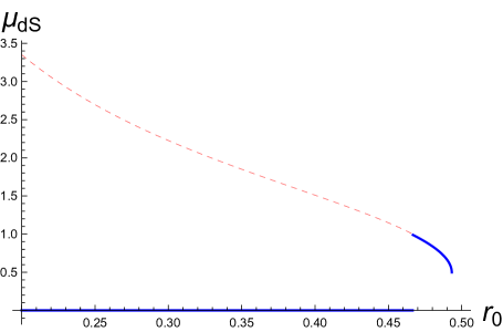
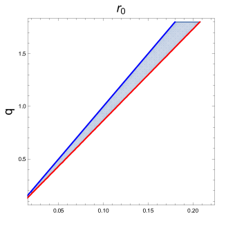
This region is situated closely to the critical charge, which means that large chemical potential restores chaotic behavior for cold enough CFT in de Sitter.
It is interesting to compare these results with the black hole with hyperbolic asymptotic boundary which can be obtained by analytical continuation . In contrast with the space of positive curvature where the chemical potential restores real-valued butterfly velocity one can observe from Fig.2 the opposite effect (i.e. for some values of becomes complex-valued).
3 Comparison with other models, related phenomena, and discussion
In the previous section, we have shown the degeneration of the butterfly velocity for the CFT at fixed local temperature propagating in the de Sitter universe with temperature . This butterfly velocity is inversely proportional to some parameter , where is the function of and . We find that for all values of and the butterfly velocity is complex-valued. On the other hand, we find that the chemical potential restores healthy positive butterfly velocity for a small enough temperature. In contrast to this for hyperbolic boundary, chemical potential creates some region of where butterfly velocity is complex-valued and vanishing for some finite . Also, it is worth noticing, that the Euclidean can be rewritten as an ordinary dimensional sphere in appropriate coordinate system. Thus the results obtained in this note can be considered as facts about CFT on the sphere.
To understand the quantitative picture of this chaotic spreading disappearance, one has to make calculations in higher-dimensional CFT at a finite temperature in the de Sitter background. Instead of doing this, let us try to understand this result from the viewpoint of different phenomena taking place in the de Sitter space and construct the qualitative picture of its chaotic properties
-
•
As the non-equilibrium processes like the thermalization in holographic CFT (which are chaotic) should be accompanied somehow with the chaotic spreading, it is worth noticing the following result closely related to shock wave solutions. In de Sitter space, the black hole formation from the shock wave collisions is also sensitive to the values of Hubble parameter as it was shown in Arefeva:2009oun ; Arefeva:2009pxq ; Arefeva:2011bcf ; for some range of and shock waves energies the black hole formation is prohibited. From the viewpoint of the dual theory, this can be interpreted as the impossibility of thermalization and consequently partial disappearance of the chaotic properties333 The butterfly velocity and OTOC in the dual of dynamical has been discussed in the context of correspondence Aalsma:2020aib ; Geng:2020kxh ; Anninos:2018svg and cosmology Choudhury:2020yaa ; Haque:2020pmp ; Bhargava:2020fhl . .
-
•
The butterfly velocity defines the effective lightcone constraining the spread of chaotic correlations after the scrambling time . In general, the effect of chaos decrease or disappearance is expected because positively curved manifolds like are “antichaotic” cousins of ( for example, in the sense of the geodesic behavior). However, the sharp transition to the degenerate complex-valued butterfly velocity indicates the presence of strong quantum effects. The process inside the effective lightcone defined by can be thought of as the operator spreading effect resembling the branching diffusion Roberts:2018mnp , which is influenced by the effect of dilution/concentration by curved spacetime.
-
•
In some sense, a very similar effect that resembles the situation with the butterfly velocity is the Schwinger effect when the particles in de Sitter are created from the external electric field. In this process, particles and antiparticles exhibit the competing influence of electric field and the geometric properties of dS. The presence of different scales (de Sitter scale, particle mass, and electric field) sets different regimes of electric current.
-
•
The analogy with the Schwinger effect and setting down different regimes of “conductivity” and current is supported by the proportionality of charge and thermal diffusion constant to a butterfly velocity established in Blake:2016wvh ; Blake:2017qgd for holographic field theories.
-
•
The example of how the chemical potential enhances particle production in cosmological setup is given in Bodas:2020yho ; Sou:2021juh . In general, the chemical potential allows the production of large mass particles, which should carry some chaotic imprint if being observed in the experimental setup.
It would be interesting to extend these results on the case when the boundary manifold is de Sitter and not the product of and as in our setting. Also, it is interesting to understand what happens when de Sitter is dynamical, i.e. to embed pole-skipping setup in correspondence (we address this issue in forthcoming paper).
Acknowledgements
This work is supported by the Russian Science Foundation under grant 20-12-00200. I would like to thank Viktor Jahnke, Juan Pedraza, and Saso Grozdanov for their comments on this paper and correspondence.
References
- (1) A. Einstein, Zum quantensatz von Sommerfeld und Epstein. Verh. Deutsch. Phys. Ges., 19, 82-92, (1917).
- (2) Martin C., Gutzwiller ”The geometry of quantum chaos.” Physica Scripta 1985.T9 (1985): 184.
- (3) A. I., Larkin, Y. N. Ovchinnikov, Y. N. (1969). Quasiclassical method in the theory of superconductivity. Sov Phys JETP, 28(6), 1200-1205.
- (4) S. H. Shenker and D. Stanford, JHEP 03, 067 (2014) doi:10.1007/JHEP03(2014)067 [arXiv:1306.0622 [hep-th]].
- (5) D. A. Roberts, D. Stanford and L. Susskind, JHEP 03, 051 (2015) doi:10.1007/JHEP03(2015)051 [arXiv:1409.8180 [hep-th]].
- (6) S. H. Shenker and D. Stanford, JHEP 12, 046 (2014) doi:10.1007/JHEP12(2014)046 [arXiv:1312.3296 [hep-th]].
- (7) J. Maldacena, S. H. Shenker and D. Stanford, “A bound on chaos,” JHEP 1608, 106 (2016) [arXiv:1503.01409 [hep-th]].
- (8) S. H. Shenker and D. Stanford, JHEP 05, 132 (2015) [arXiv:1412.6087 [hep-th]].
- (9) M. Blake, “Universal Charge Diffusion and the Butterfly Effect in Holographic Theories,” Phys. Rev. Lett. 117, no.9, 091601 (2016) [arXiv:1603.08510 [hep-th]].
- (10) M. Blake, R. A. Davison and S. Sachdev, “Thermal diffusivity and chaos in metals without quasiparticles,” Phys. Rev. D 96, no.10, 106008 (2017) [arXiv:1705.07896 [hep-th]].
- (11) D. A. Roberts and B. Swingle, “Lieb-Robinson Bound and the Butterfly Effect in Quantum Field Theories,” Phys. Rev. Lett. 117, no.9, 091602 (2016) [arXiv:1603.09298 [hep-th]].
- (12) V. Jahnke, “Recent developments in the holographic description of quantum chaos,” Adv. High Energy Phys. 2019, 9632708 (2019) [arXiv:1811.06949 [hep-th]].
- (13) Y. Ahn, V. Jahnke, H. S. Jeong and K. Y. Kim, “Scrambling in Hyperbolic Black Holes: shock waves and pole-skipping,” JHEP 10, 257 (2019) doi:10.1007/JHEP10(2019)257 [arXiv:1907.08030 [hep-th]].
- (14) Anosov, D. V. (1967). Geodesic flows on closed Riemannian manifolds of negative curvature. Trudy Matematicheskogo Instituta Imeni VA Steklova, 90, 3-210.
- (15) Y. Ahn, V. Jahnke, H. S. Jeong, K. Y. Kim, K. S. Lee and M. Nishida, “Pole-skipping of scalar and vector fields in hyperbolic space: conformal blocks and holography,” JHEP 09, 111 (2020) doi:10.1007/JHEP09(2020)111 [arXiv:2006.00974 [hep-th]].
- (16) J. B. Hartle and S. W. Hawking, “Wave Function of the Universe,” Phys. Rev. D 28, 2960-2975 (1983)
- (17) E. Witten, “Quantum gravity in de Sitter space,” [arXiv:hep-th/0106109 [hep-th]].
- (18) A. Strominger, “The dS / CFT correspondence,” JHEP 10, 034 (2001) [arXiv:hep-th/0106113 [hep-th]].
- (19) D. S. Ageev and I. Y. Aref’eva, “When things stop falling, chaos is suppressed,” JHEP 01, 100 (2019) [arXiv:1806.05574 [hep-th]].
- (20) D. S. Ageev, “Holography, quantum complexity and quantum chaos in different models,” EPJ Web Conf. 191, 06006 (2018) [arXiv:1902.02245 [hep-th]].
- (21) R. Emparan, “AdS membranes wrapped on surfaces of arbitrary genus,” Phys. Lett. B 432, 74-82 (1998) [arXiv:hep-th/9804031 [hep-th]].
- (22) D. Birmingham, “Topological black holes in Anti-de Sitter space,” Class. Quant. Grav. 16, 1197-1205 (1999) doi:10.1088/0264-9381/16/4/009 [arXiv:hep-th/9808032 [hep-th]].
- (23) R. G. Cai and K. S. Soh, “Topological black holes in the dimensionally continued gravity,” Phys. Rev. D 59, 044013 (1999) [arXiv:gr-qc/9808067 [gr-qc]].
- (24) A. Chamblin, R. Emparan, C. V. Johnson and R. C. Myers, “Charged AdS black holes and catastrophic holography,” Phys. Rev. D 60, 064018 (1999) [arXiv:hep-th/9902170 [hep-th]].
- (25) D. Marolf, M. Rangamani and M. Van Raamsdonk, “Holographic models of de Sitter QFTs,” Class. Quant. Grav. 28, 105015 (2011) [arXiv:1007.3996 [hep-th]].
- (26) W. Fischler, P. H. Nguyen, J. F. Pedraza and W. Tangarife, “Holographic Schwinger effect in de Sitter space,” Phys. Rev. D 91, no.8, 086015 (2015) [arXiv:1411.1787 [hep-th]].
- (27) W. Fischler, S. Kundu and J. F. Pedraza, “Entanglement and out-of-equilibrium dynamics in holographic models of de Sitter QFTs,” JHEP 07, 021 (2014) [arXiv:1311.5519 [hep-th]].
- (28) W. Fischler, P. H. Nguyen, J. F. Pedraza and W. Tangarife, “Fluctuation and dissipation in de Sitter space,” JHEP 08, 028 (2014) [arXiv:1404.0347 [hep-th]].
- (29) K. Sfetsos, “On gravitational shock waves in curved space-times,” Nucl. Phys. B 436, 721-745 (1995) doi:10.1016/0550-3213(94)00573-W [arXiv:hep-th/9408169 [hep-th]].
- (30) A. Bodas, S. Kumar and R. Sundrum, “The Scalar Chemical Potential in Cosmological Collider Physics,” JHEP 02, 079 (2021) doi:10.1007/JHEP02(2021)079 [arXiv:2010.04727 [hep-ph]].
- (31) C. M. Sou, X. Tong and Y. Wang, “Chemical-Potential-Assisted Particle Production in FRW Spacetimes,” [arXiv:2104.08772 [hep-th]].
- (32) I. Y. Aref’eva, A. A. Bagrov and E. A. Guseva, “Critical Formation of Trapped Surfaces in the Collision of Non-expanding Gravitational Shock Waves in de Sitter Space-Time,” JHEP 12, 009 (2009) [arXiv:0905.1087 [hep-th]].
- (33) I. Y. Aref’eva, A. A. Bagrov and L. V. Joukovskaya, “Critical Trapped Surfaces Formation in the Collision of Ultrarelativistic Charges in (A)dS,” JHEP 03, 002 (2010) doi:10.1007/JHEP03(2010)002 [arXiv:0909.1294 [hep-th]].
- (34) I. Y. Aref’eva, A. A. Bagrov and L. V. Joukovskaya, “Several aspects of applying distributions to analysis of gravitational shock waves in general relativity,” St. Petersburg Math. J. 22, no.3, 337-337 (2011) doi:10.1090/S1061-0022-2011-01144-6
- (35) D. A. Roberts, D. Stanford and A. Streicher, “Operator growth in the SYK model,” JHEP 06, 122 (2018) doi:10.1007/JHEP06(2018)122 [arXiv:1802.02633 [hep-th]].
- (36) L. Aalsma and G. Shiu, “Chaos and complementarity in de Sitter space,” JHEP 05, 152 (2020), [arXiv:2002.01326 [hep-th]].
- (37) H. Geng, “Non-local entanglement and fast scrambling in de-Sitter holography,” Annals Phys. 426, 168402 (2021), [arXiv:2005.00021 [hep-th]].
- (38) D. Anninos, D. A. Galante and D. M. Hofman, “De Sitter horizons & holographic liquids,” JHEP 07, 038 (2019) [arXiv:1811.08153 [hep-th]].
- (39) S. Choudhury, “The Cosmological OTOC: Formulating new cosmological micro-canonical correlation functions for random chaotic fluctuations in Out-of-Equilibrium Quantum Statistical Field Theory,” Symmetry 12, no.9, 1527 (2020) [arXiv:2005.11750 [hep-th]].
- (40) P. Bhargava, S. Choudhury, S. Chowdhury, A. Mishara, S. P. Selvam, S. Panda and G. D. Pasquino, “Quantum aspects of chaos and complexity from bouncing cosmology: A study with two-mode single field squeezed state formalism,” [arXiv:2009.03893 [hep-th]].
- (41) S. S. Haque and B. Underwood, “Squeezed out-of-time-order correlator and cosmology,” Phys. Rev. D 103, no.2, 023533 (2021) [arXiv:2010.08629 [hep-th]].
- (42) S. Grozdanov, K. Schalm and V. Scopelliti, “Black hole scrambling from hydrodynamics,” Phys. Rev. Lett. 120, no.23, 231601 (2018) [arXiv:1710.00921 [hep-th]].
- (43) M. Blake, R. A. Davison, S. Grozdanov and H. Liu, “Many-body chaos and energy dynamics in holography,” JHEP 10, 035 (2018) doi:10.1007/JHEP10(2018)035 [arXiv:1809.01169 [hep-th]].