Spectroscopic Confirmation of two Extremely Massive Protoclusters BOSS1244 and BOSS1542 at $z=2.24$

Abstract

We present spectroscopic confirmation of two new massive galaxy protoclusters at $z=2.24\pm 0.02$, BOSS1244 and BOSS1542, traced by groups of Coherently Strong Ly$\alpha$ Absorption (CoSLA) systems imprinted in the absorption spectra of a number of quasars from the Sloan Digital Sky Survey III (SDSS III) and identified as overdensities of narrowband-selected H$\alpha$ emitters (HAEs). Using MMT/MMIRS and LBT/LUCI near-infrared (NIR) spectroscopy, we confirm 46 and 36 HAEs in the BOSS1244 ($\sim 55\,$arcmin²) and BOSS1542 ($\sim 61\,$arcmin²) fields, respectively. BOSS1244 displays a South-West (SW) component at $z=2.230\pm 0.002$ and another North-East (NE) component at $z=2.246\pm 0.001$ with the line-of-sight velocity dispersions of $405\pm 202$ km s^-1 and $377\pm 99$ km s^-1, respectively. Interestingly, we find that the SW region of BOSS1244 contains two substructures in redshift space, likely merging to form a larger system. In contrast, BOSS1542 exhibits an extended filamentary structure with a low velocity dispersion of $247\pm 32$ km s^-1 at $z=2.241\pm 0.001$, providing a direct confirmation of a large-scale cosmic web in the early Universe. The galaxy overdensities $\delta_{\rm g}$ on the scale of 15 cMpc are $22.9\pm 4.9$, $10.9\pm 2.5$, and $20.5\pm 3.9$ for the BOSS1244 SW, BOSS1244 NE, and BOSS1542 filament, respectively. They are the most overdense galaxy protoclusters ($\delta_{\rm g}>20$) discovered to date at $z>2$. These systems are expected to become virialized at $z\sim 0$ with a total mass of $M_{\rm SW}=(1.59\pm 0.20)\times 10^{15}$ $M_{\sun}$, $M_{\rm NE}=(0.83\pm 0.11)\times 10^{15}$ $M_{\sun}$ and $M_{\rm filament}=(1.42\pm 0.18)\times 10^{15}$ $M_{\sun}$, respectively. Our results suggest that the dense substructures of BOSS1244 and BOSS1542 will eventually evolve into the Coma-type galaxy clusters or even larger. Together with BOSS1441 described in Cai et al. (2017a), these extremely massive overdensities at $z=2-3$ exhibit different morphologies, indicating that they are in different assembly stages in the formation of early galaxy clusters. Furthermore, there are two quasar pairs in BOSS1441, one quasar pair in BOSS1244 and BOSS1542, CoSLAs detected in these quasar pairs can be used to trace the extremely massive large-scale structures of the Universe.

1 Introduction

In a cold dark matter universe dominated by a cosmological constant ($\Lambda$CDM), theories of structure formation predict that galaxy formation preferentially occurs along large-scale filamentary or sheet-like overdense structures in the early universe. The intersections of such filaments host “protoclusters” (van Albada, 1961; Peebles, 1970; Sunyaev & Zeldovich, 1972), which evolve into viralized massive galaxy clusters at the present epoch (e.g., Bond et al., 1996; Cen & Ostriker, 2000; Muldrew et al., 2015; Overzier, 2016). Protoclusters provide ideal laboratories to study galaxy properties in dense environments and the environment dependence of galaxy formation and evolution in the early universe. Galaxies in dense environments appear to be more massive, with lower specific Star Formation Rates (SFRs), and their growth in the early universe is accelerated in the sense that protocluster galaxies formed most of their stars earlier than field galaxies (Hatch et al., 2011).

Present-day massive galaxy clusters are dominated by spheroidal galaxies with low star formation activities while those in the general fields are mostly still actively forming stars (Skibba et al., 2009; Collins et al., 2009; Santos et al., 2014, 2015). These galaxy clusters are key to tracing the formation of the most massive dark matter halos, galaxies and supermassive black holes (SMBHs) (Springel et al., 2005). Cluster galaxies show a tight “red sequence” and obey the “morphology-density” relation, indicating the impact of dense environments on the star formation activities of the inhabitants (Visvanathan & Sandage, 1977; Dressler, 1980; Bower et al., 1992; Goto et al., 2003). To understand the physical processes that drive both the mass build-up in galaxies and the quenching of star formation, we need to investigate galaxies and their surrounding gas within and around the precursors of present-day massive galaxy clusters$-$protoclusters at $z>2$. The transition period before protocluster member galaxies began to quench and evolved to the massive clusters currently observed is a crucial phase to study their physical properties and the mechanisms driving their evolution (Kartaltepe et al., 2019).

In the last decades, protoclusters at $z>2$ have been successfully discovered and several techniques for tracing the overdense regions have been developed. These include performing “blind” deep surveys (of H$\alpha$ emitters (HAEs), Ly$\alpha$ emitters (LAEs), Lyman break galaxies (LBGs) and photo-z selected galaxies) (Steidel et al., 1998, 2000, 2003; Shimasaku et al., 2003; Steidel et al., 2005; Ouchi et al., 2005; Toshikawa et al., 2012; Chiang et al., 2014; Le Fèvre et al., 2015; Planck Collaboration et al., 2015; Toshikawa et al., 2016; Jiang et al., 2018; Lemaux et al., 2018; Shi et al., 2020) and targeting rare massive halo tracers, e.g., quasars, radio galaxies, Ly$\alpha$ blobs (LABs) and submilimeter galaxies (SMGs; Pascarelle et al., 1996; Pentericci et al., 2000; Kurk et al., 2000, 2004a; Venemans et al., 2002, 2004, 2005, 2007; Daddi et al., 2009; Kuiper et al., 2011; Hatch et al., 2011, 2014; Hayashi et al., 2012; Cooke et al., 2014, 2016; Husband et al., 2016; Casasola et al., 2018). The former is limited by their relatively small survey volumes, while the latter may suffer from the strong selection biases and small duty cycles (Cai et al., 2016, 2017a). A promising selection technique for protoclusters is through the group of gas absorption systems along multiple sightlights to background quasars or galaxies (Lee et al., 2014a; Stark et al., 2015; Cai et al., 2016; Miller et al., 2019).

Cai et al. (2016) demonstrated that the extremely massive overdensities at $z=2-3$ traced by groups of Coherently Strong intergalactic Ly$\alpha$ absorption (CoSLA). This approach utilizes the largest library of quasar spectra, such as those from the SDSS-III Baryon Oscillations Spectroscopic Survey (BOSS), to locate extremely rare, strong H I absorption from the IGM and select candidates for the most massive protoclusters (e.g., Liang et al., 2021). Cai et al. (2016) used cosmological simulations to show that the correlation between IGM Ly$\alpha$ optical depth and matter overdensities peaks on the scale of $10-30$ $h^{-1}$ comoving Mpc (cMpc), finding that the strongest IGM Ly$\alpha$ absorption systems trace 4$\sigma$ extreme tail of mass overdensities on 15 $h^{-1}$ cMpc (Lee et al., 2018; Mukae et al., 2020). This technique is referred as MApping the Most Massive Overdensity Through Hydrogen (MAMMOTH). Using MAMMOTH technique, the massive BOSS1441 overdensity at $z=2.32\pm 0.02$ is selected from the early data release of SDSS-III BOSS. The LAE overdensity in BOSS1441 is $10.8\pm 2.6$ on a 15 cMpc scale, which could collapse to a massive cluster with $\geq 10^{15}$ $M_{\sun}$ at the present day (Cai et al., 2017a). Furthermore, an ultra-luminous Enormous Ly$\alpha$ nebulae (also known as MAMMOTH-1) with a size of $\sim 442$ kpc at $z=2.32$ is discovered at the density peak of BOSS1441 (Cai et al., 2017b), which is used to trace the densest and most active regions of galaxy and cluster formation (e.g., Cantalupo et al., 2014; Arrigoni Battaia et al., 2015; Borisova et al., 2016; Cai et al., 2018, 2019).

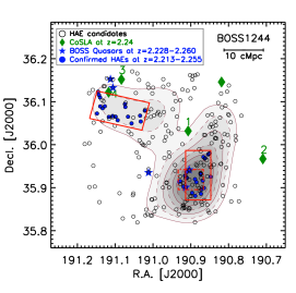
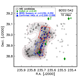
Figure 1: Slitmask regions of MMT/MMIRS (red boxes: $4\arcmin\times 6\farcm 9$) and LBT/LUCI (red dot-dashed boxes: $4\farcm 0\times 2\farcm 8$) in BOSS1244 (left) and BOSS1542 (right). BOSS1244-mask1 and BOSS1244-mask2 are located in the SW and NE regions, respectively. The dashed blue box in the right panel refers to BOSS1542-mask1, which was not observed due to the bad weather conditions. These structures are traced by groups of Ly$\alpha$ absorption systems (green diamonds) and BOSS quasars (blue stars) at the redshift of $z=2.24\pm 0.02$. The black circles are the selected HAE candidates and the filled circles show the spectroscopically confirmed HAEs through MMT/MMIRS and LBT/LUCI NIR spectroscopy. The solid and dashed lines represent contours of the density map of HAEs. A galaxy number density of 0.2 per arcmin² is adopted as the contour interval and the inner density peak reaches $\sim 2\,$ arcmin^-2.

Two more CoSLA candidates selected using the MAMMOTH technique, BOSS1244 and BOSS1542, have been confirmed to be extremely massive overdensities within 20 $h^{-1}$ cMpc at $z=2.24\pm 0.02$ using the H$\alpha$ Emitter (HAE) candidates identified from near-infrared (NIR) narrow-band imaging (Zheng et al., 2021). Currently, only a few protoclusters at $z\geq 2$ are identified by NIR spectroscopy of HAEs. For example, the well-studied PKS 1138 at $z=2.16$ and USS 1558 at $z=2.53$ protoclusters associated with radio galaxy environments will evolve into the massive galaxy clusters with masses of $\sim 10^{15}\,M_{\sun}$ at $z\sim 0$ (Kurk et al., 2004a; Hayashi et al., 2012; Shimakawa et al., 2014, 2018a, 2018b). Tanaka et al. (2011) reported a protocluster associated with the radio galaxy 4C 23.56 at $z=2.48$ had $\sim 5-6$ times excess of HAEs from the general field, which might evolve into a galaxy cluster with the present-day mass of $>10^{14}\,M_{\sun}$. Darvish et al. (2020) confirmed a protocluster CC2.2 at $z=2.23$ with a present-day mass of $9.2\times 10^{14}\,M_{\sun}$ through the NIR spectroscopy of HAEs. Recently, Koyama et al. (2021) presented a $Planck$-selected protocluster at $z=2.16$ associated with an overdensity of HAEs, six HAEs at $z=2.150-2.164$ were identified through spectroscopy. Although they do not calculate the present-day mass, we estimate that the fate of the protocluster may be a Virgo-type galaxy cluster ($\sim 10^{14}\,M_{\sun}$) at present day based on the volume they gave.

In this paper, we present NIR spectroscopic followup observations of these HAE candidates, quantitatively showing that BOSS1244 and BOSS1542 are indeed extremely overdense, and will collapse to two extremely massive clusters (like Coma cluster or even larger) at $z\sim 0$. We also use these identified HAEs to analyze dynamical properties (e.g., velocity dispersion, dynamical mass) and evolutionary stages of two overdensities. Furthermore, we estimate the total mass of the two overdensities to the present-day based on the galaxy overdensities. The physical properties of HAEs in BOSS1244 and BOSS1542 will be presented in future work (Shi, D.D. et al. in preparation). The spectroscopic observations and data reduction are descried in Section 2. In Section 3, we present the main analyses and results, and discuss the implications for the extremely overdense regions in Section 4. Our conclusions are summarized in Section 5. Throughout this paper, we adopt the cosmological parameters of $\Omega_{\rm M}=0.3$, $\Omega_{\rm\Lambda}=0.7$ and $H\rm_{0}=70$ km s^-1 Mpc^-1 and magnitudes are presented in the AB system unless otherwise specified. At $z=2.24$, 1$\arcmin$ corresponds to 0.495 physical Mpc (pMpc) and 1.602 comoving Mpc (cMpc), respectively.

2 Observations and Data Reductions

Zheng et al. (2021) carried out deep NIR imaging observations with Canada$-$France$-$Hawaii Telescope (CFHT) through the narrowband (NB) $H_{\rm 2}S1$ and broadband (BB) $K_{\rm s}$ filters to identify emission-line objects. The NB technique selects objects with an excess of emission at $\lambda=2.13\,\mu$m. The emission-line may be [O III] from emitters at $z\simeq 3.25$, [O II] at $z\simeq 4.71$ or Pa$\alpha$/Pa$\beta$ at $z\simeq 0.14$/0.66 and [S III] at $z\simeq 1.23$/1.35 (e.g., Geach et al., 2008; Sobral et al., 2012). In total, 244/223 line emitters are selected with rest-frame $EW\textgreater 45$ Å  and $H_{2}S1\textless 22.5$ mag over the effective area of 417/399 arcmin² in BOSS1244/BOSS1542. As shown in Zheng et al. (2021), about 80% of these emitters are HAEs at $z=2.24\pm 0.02$, and the H$\alpha$ luminosity functions (LF) can be derived in a statistical manner. Their results show that the shape of the H$\alpha$ LF of BOSS1244 agrees well with that of the general fields, while in BOSS1542, the LF exhibits a prominent excess at the high end, likely caused by the enhanced star formation or AGN activity. We perform NIR spectroscopic observations to confirm the extremely overdense nature of two regions and better quantify their overdensities.

Table 1: MMT/MMIRS and LBT/LUCI NIR spectroscopic observations for the BOSS1244 and BOSS1542 fields.

Field/SlitMask	Nobj	R.A.	Decl.	P.A.	Grism+Filter	Exp.time	ObsDate	Seeing
		(J2000.0)	(J2000.0)	(deg)		(second)		Average ($\arcsec$)
BOSS1244/mask1	19/28	$12^{h}43^{m}31.28^{s}$	$+35\arcdeg 55\arcmin 44\farcs 38$	$180$	$K3000+K\rm spec$	12,024	2017/06/14,18	1.16
BOSS1244/mask2	18/18	$12^{h}44^{m}21.26^{s}$	$+36\arcdeg 04\arcmin 44\farcs 62$	$-104$	$K3000+K\rm spec$	12,024	2017/06/11,12,17	1.05
BOSS1542/mask1	0/26	$15^{h}42^{m}53.20^{s}$	$+38\arcdeg 52\arcmin 06\farcs 50$	$-11$	$K3000+K\rm spec$	…	…	…
BOSS1542/mask2	14/23	$15^{h}42^{m}41.78^{s}$	$+39\arcdeg 01\arcmin 07\farcs 62$	$-13$	$K3000+K\rm spec$	7,236	2017/05/14	0.83
BOSS1244/mask	8/18	$12^{h}43^{m}34.76^{s}$	$+35\arcdeg 55\arcmin 07\farcs 33$	$90$	$HK\rm spec$$+HK\rm spec$	5,256	2017/04/13	$\leq 1.2$
BOSS1542/mask1	8/14	$15^{h}42^{m}51.80^{s}$	$+38\arcdeg 49\arcmin 49\farcs 37$	$30$	$HK\rm spec$$+HK\rm spec$	7,668	2017/04/12	$\leq 1.2$
BOSS1542/mask2	7/9	$15^{h}42^{m}48.18^{s}$	$+38\arcdeg 53\arcmin 35\farcs 39$	$0$	$HK\rm spec$$+HK\rm spec$	6,480	2017/04/13	$\leq 1.2$
BOSS1542/mask3	7/13	$15^{h}42^{m}37.66^{s}$	$+38\arcdeg 57\arcmin 59\farcs 07$	$-25$	$HK\rm spec$$+HK\rm spec$	5,508	2017/04/13	$\leq 1.2$

Note. — Above double lines are the MMT/MMIRS observations, below the double lines are the observations in LBT/LUCI. The number to the left of slash in column (2) is the number of successfully confirmed galaxies, and the number to the right of slash in column (2) is total number of HAE candidates in the slitmask. No observations in MMT/MMIRS BOSS1542/mask1 due to bad weather.

2.1 MMT/MMIRS Spectroscopy

Spectroscopic observations of the HAE candidates in the density peak regions of BOSS1244 and BOSS1542 are carried out using the Multiple Mirror Telescope (MMT) and Magellan Infrared Spectrograph (MMIRS; McLeod et al., 2012), mounted on the MMT telescope (PI: Zheng, X.Z.) in 2017. MMIRS is a near infrared (NIR) imager with an imaging Field of View (FOV) $6\farcm 9\times 6\farcm 9$ and multi-object spectrograph (MOS) over $4\arcmin\times 6\farcm 9$. We use the “xfitmask” program to design our slit masks. There are two masks designed in each field. The red rectangles in Figure 1 are the observed slit mask regions of two fields and the dashed blue rectangle in BOSS1542 is the unobserved slit mask region due to the bad weather. A slit width of 1$\farcs$0 and a slit length of 7$\farcs$0 are adopted for observing our science targets, and the low noise gain (0.95) is used. The targets are prioritized based on their $K_{\rm s}$ magnitudes with 0$\farcs$7 aperture: we rank the highest, medium and lowest priorities to objects with $K_{\rm s}$ magnitudes in the range of 18.9$-$22.8, 22.8$-$24.3, 24.3$-$25.0 mag, respectively. The $K3000$ grism and $K\rm spec$ filter are used to take spectra over the wavelength coverage of 1.90$-$2.45 $\micron$ (Chilingarian et al., 2015). With these configurations, the resolution of $1\farcs 0$ slit width in the $K3000$ grism and $K\rm spec$ filter corresponds to $R=1200$. We dither along the slit between individual 300 s exposures. Three out of four masks were successfully observed under the average seeing conditions of $0\farcs 83-1\farcs 16$ with the total integration time of 8.69 hrs in Semester 2017A. Four to five alignment stars with $13.5<H<16\,$mag (Vega) were chosen in our masks. In addition, we observed A0V stars in each mask at a similar airmass in order to derive the spectral response function and remove atmospheric absorption pattern from spectra. Details of MMIRS slit masks are summarized in Table 1.

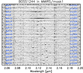
Figure 2: 2D spectra of 19 HAEs in BOSS1244 observed via MMT/MMIRS slit mask1. Skyline residuals are marked as vertical lines with a higher noise level. The slit and spectrum number are labeled. Almost all spectra (excluding slit-23 and slit-30) have only one emission line, and their continua are barely detected. The spectrum of slit-13 is consistent with a quasar with a broad H$\alpha$ emission line.

We use the standard MMIRS data reduction pipeline to process our MMIRS data (Chilingarian et al., 2015). Four point dither pattern ($ABA^{\prime}B^{\prime}:+1\farcs 8-1\farcs 4,+1\farcs 4-1\farcs 8$) mode was adopted in our MOS mask observations. The major steps of data reduction include nonlinearity correction, dark subtraction, spectral tracing, flat-fielding, wavelength calibration, sky subtraction and telluric correction. Two-dimensional (2D) spectra were extracted from the original frames without resampling after tracing and distortion mapping, and we set per-slit normalization for flat-fielding due to the imperfect illumination of the detector plane. We use airglow $OH$ lines for wavelength calibration given our faint targets and long exposure time ($300\,$s), but internal arc frames will be used if the $OH$ based computation fails. The sky subtraction is done using a technique modified from the original one given in Kelson (2003). For telluric correction, the pipeline computes the empirical atmosphere transmission function by the ratio of the observed telluric standard star spectrum and a synthetic stellar atmosphere of star. The empirical transmission function is corrected for the airmass difference between the observations of telluric standard and the science target. The 1D spectra are extracted from the reduced 2D spectra at every slit. The 2D/1D spectra with sky subtracted and telluric corrected are obtained.

The NB excess fluxes are used to perform the absolute flux calibration for our spectral lines considering no slit stars are included in each slit mask. The object fluxes are calculated using the photometric magnitude at $H_{2}S1$- and $K_{\rm s}$-band with the equation (2) described in Zheng et al. (2021). We then convolve NB filter with the 1D spectra of Gaussian fitting to calculate total electrons, and correct the scaling factors ($\sim 2-5\times 10^{-22}$) of 1D spectra at every target. We also use alignment stars (marked with “BOX”) to check the absolute flux calibration, and the scaling factors are $\sim 5\times 10^{-22}$ in the $H_{2}S1$ and $K_{\rm s}$ bands, which is $1-3$ times larger than the aforementioned method. This may be mainly due to the large slit width ($4\arcsec$) of alignment stars so that more light is collected. Therefore, we use NB excess flux to take the absolute flux calibration for our final calibrated spectra.

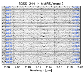
Figure 3: 2D spectra of 18 HAEs in BOSS1244 observed via MMT/MMIRS slit mask2. Skyline residuals are marked as vertical lines with a higher noise level. The slit and spectrum number are labeled. The spectra of slit 9, 20 and 21 show multiple lines. The rest exhibit only a single emission line. Continuum is barely visible in all spectra.

In total 46 HAE targets in BOSS1244 (two masks) and 23 HAE targets in BOSS1542 (one mask) are covered in the MMT/MMIRS observations. We use a single Gaussian function to fit the emission line and measure the observed wavelength through H$\alpha$ line (the rest frame H$\alpha$ emission line is 6564.61Å in vacuum) to derive the redshift of HAEs. If multiple components are detected, we will use multiple Gaussians in multiple regions to fit them. The equation $z=\lambda_{\rm obs}/\lambda_{\rm rest}-1$ is used to compute the redshift, where $\lambda_{\rm rest}$ is the rest-frame wavelength and $\lambda_{\rm obs}$ is the observe-frame wavelength.

Figure 4: 2D spectra of 14 HAEs in BOSS1542 observed via MMT/MMIRS slit mask2. Skyline residuals are visible as vertical lines with a higher noise level. The slit and spectrum ID are indicated. We note that the spectrum of slit-27 from an [O III] emitter at $z=3.302$.

2.2 LBT/LUCI Spectroscopy

To increase the sample size of spectroscopically-confirmed HAEs, three masks (36 targets) in BOSS1542 and one mask (18 targets) in BOSS1244 were observed using the LBT Utility Camera in the Infrared (LUCI) mounted on the Large Binocular Telescope (LBT) in semester 2017A (PI: Fan, X.). The relatively small dot-dashed red boxes in Figure 1 are the observed slit mask regions of two fields. LUCI is able to provide imaging, longslit spectroscopy, and MOS spectroscopy over a FOV of four square arcminutes. We choose MOS spectroscopy and the slit masks are designed through the LMS software. Six alignment stars are used to correct telescope pointing and instrument rotation angle. The N1.8 camera with $4\farcm 0\times 2\farcm 8$ FOV, $HK\rm spec$ grating with low resolution ($R=1900$) and $HK\rm spec$ filter are selected. Slits of 1$\farcs$0$\times$8$\farcs$0, 0$\farcs$5 $\times$0$\farcs$5 and 4$\farcs$0$\times$4$\farcs$0 are used for our targets, alignment stars, guide stars, respectively. These observations were observed under the good seeing ($<1\farcs 2$) conditions and each exposure takes 240 seconds. The total integration time in every mask is listed in Table 1.

Our LBT data were reduced using $Flame$ (Belli et al., 2018), a flexible data reduction pipeline written in Interactive Data Language (IDL) for NIR and optical spectroscopic data. We carried out data reduction following the reduction procedure given in the manual of $Flame$. We briefly describe the key steps below. Firstly, we set the inputs, initialize and create data structure. The reduction includes diagnostics of the observing conditions, calibrations on each of the science frames (including cosmic rays, bad pixels, dark frames and flat-fields), slit identification and cutout extraction, wavelength calibration, illumination correction, sky subtraction, and the extraction of 1D spectra from reduced and combined frames. More details about the pipeline can be found in the Belli et al. (2018). We also used NB excess flux to derive the absolute flux calibration. The method of calculating the redshifts of HAE candidates is the same as MMT/MMIRS, which is described in Section 2.1.

3 Results and Analysis

3.1 Spectroscopic Confirmation of HAE Candidates

We detect emission lines in 37 of 46 HAE candidates in BOSS1244 with spectra obtained from MMT/MMIRS. All of them are confirmed to be HAEs in redshift range of $2.213<z<2.255$. Note that most spectra show only one emission line and weak or no continuum. We further check these objects using the $BzK$ diagram from Daddi et al. (2004), finding that they all fall into the region occupied by galaxies at $z>1.4$. We thus confirm that the detected lines are H$\alpha$ and these objects are HAEs.

Our MMT/MMIRS observations in BOSS1244 gave an overall success rate of 80% (37 in 46) in identifying HAEs. The detection rate is $\sim$68% (19 in 28) and 100% (all 18) in mask1 and mask2 of BOSS1244, respectively. The difference in detection rate is largely caused by observational conditions: mask2 was taken under a better condition than mask1 (see Table 1), although their integration times are the same and targets’ line fluxes are similar. There may be some main reasons for the undetected targets in mask1: (a) some are too faint (NB$>$22.0 mag) to be detected; (b) large seeing ($\sim$ 1$\farcs$2) conditions smear the signals of faint lines below the detection limit; (c) some bright targets may not be real emission line galaxies.

Figure 5: MMT/MMIRS 1D spectra of 12 HAEs obtained from the BOSS1244 slitmasks, including one BOSS quasar. The blue line in every plot is the sky line and the vertical blue dashed line is the H$\alpha$ emission. The vertical cyan dashed line is the [NII] emission.

Figure 6: MMT/MMIRS 1D spectra of eight HAEs in BOSS1542. The bottom-right panel shows the spectrum of an [O III] emitter at z=3.302. The blue curves represent the sky emission. The vertical dashed lines mark the emission lines H$\alpha$ or [O III]$\lambda\lambda 4960,5008\rm\AA$ emission.

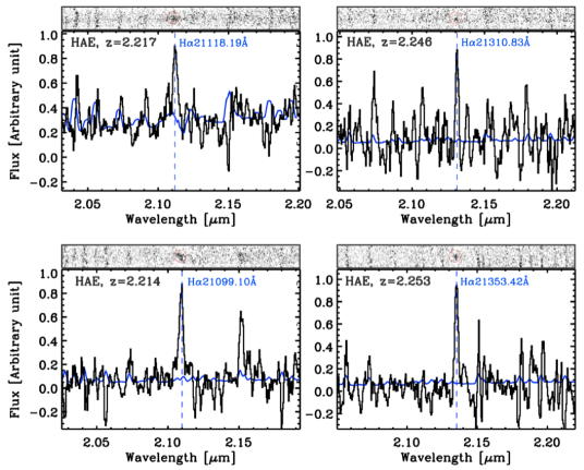
Figure 7: LBT/LUCI 1D and 2D spectra of four HAEs in BOSS1244. The blue line in each panel is the sky line and the vertical blue dashed line is the H$\alpha$ emission.

The reduced 2D spectra of HAEs in BOSS1244 are shown in Figure 2 and Figure 3. In slit mask1, slit-13 is the spectrum of a quasar with a broad emission line of full width at half maximum (FWHM)$=$4031 km s^-1. This quasar is also included in SDSS Data Release 14 Quasar catalog (DR14Q). From these spectra, only five targets (two in mask1 and three in mask2) show H$\alpha$ resolved from [N II] line. We used multiple Gaussian functions to fit them simultaneously if more than two emission lines are resolved. Figure 5 shows the H$\alpha$ lines of some HAEs from our observations.

Moreover, we obtained one mask in BOSS1244 with LBT/LUCI. Eight out of 18 (44%) HAE candidates have H$\alpha$ emission line detected. Of them, three HAEs are overlapped with MMT/MMIRS mask1, and have consistent redshifts. Figure 7 presents the extracted 1D and 2D LUCI spectra for four objects. Altogether, 46 galaxies (including 41 HAEs and 5 quasars) at $2.213<z<2.255$ in BOSS1244 are identified from our NIR observations. These spectroscopically confirmed HAEs are listed in Table A1.

For BOSS1542, we obtained one mask (23 targets in total) spectroscopic observation with MMT/MMIRS and three masks (36 targets in total) with LBT/LUCI. Using the method described before, 14 HAEs at $2.206<z<2.253$ are confirmed through MMT/MMIRS spectroscopic observations. The detection rate is 14/23 (61%), lower than that of the previous two masks in BOSS1244. We note that the mask in BOSS1542 has a shorter integration time although it was observed under a better condition. In addition, we identify slit-27 as an [O III] emitter at $z=3.302$, because [O III]$\lambda\lambda 4960,5008\rm\AA$  lines are resolved. Excluding the slit-27 target, the detection rate of HAEs is 13/23 (57%). This low detection rate in BOSS1542 is mainly due to the shorter exposure time (shown in Table 1). Similarly, we identify 22 of 36 targets at $2.215<z<2.269$ as HAEs using spectra obtained with LBT/LUCI, giving a success rate of 61%. Three HAEs observed with LBT/LUCI in BOSS1542 are quasars included in SDSS DR14Q. In total, 36 galaxies (including 33 HAEs and 3 quasars) at $2.206<z<2.269$ and one [O III] emitter at $z=3.302$ in BOSS1542 are confirmed by our NIR spectroscopic observations. These spectroscopically confirmed HAEs are listed in Table A2.

For HAEs, we calculate their redshifts based on the best-fit Gaussian profiles to the H$\alpha$ emission line and other emission lines (e.g., [O III] and [N II]). Figure 9 shows the histogram of spectroscopic redshifts in BOSS1244 and in BOSS1542, respectively. As discussed below, our spectroscopic observations confirm BOSS1244 and BOSS1542 as extreme galaxy overdensities, indicating that HAEs are an effective tracer of the overdense region of large-scale structures. We will present the physical properties of HAEs in the extremely overdense environments in a subsequent paper (Shi, D.D. et al. in preparation).

Figure 8: LBT/LUCI 1D and 2D spectra of six HAEs in BOSS1542. The blue line in each panel is the sky line and the vertical blue dashed line is the H$\alpha$ emission.

3.2 Redshift distributions of HAEs

Figure 9 shows the redshift distributions of HAEs of BOSS1244 and BOSS1542. The two overdense systems exhibit different velocity (redshift) structures. BOSS1244 presents two separated peaks in redshift distribution, indicating that there are two substructures in redshift space. We use two Gaussian profiles to fit the redshift histogram, giving two redshift peaks at $z=2.230\pm 0.002$ and $z=2.246\pm 0.001$. From the projected sky space shown in the left panel of Figure 10, there are two distinct components in sky space as well, i.e. South-West (SW) and North-East (NE) regions. The SW region seems to be connected with the NE region (shown in the left panel of Figure 1), the projected separation between them is 13$\farcm$5 ($\sim 21.6\,$cMpc at $z=2.24$). The two components are covered by our MMT/MMIRS observations. Further, we find that the SW region also shows the double peak in redshift distribution. One is at $z=2.230\pm 0.002$ and another is at $z=2.245\pm 0.001$, which is the consistent with the redshift of NE region. Moreover, from the projected sky space, the two substructures of SW region may be merging and forming a larger structure. Altogether, BOSS1244 has two distinct components both in sky and redshift space. In contrast, BOSS1542 shows a very extended filamentary structure over the scale of $\sim 14\farcm 6$, or 23.4 cMpc from South to North region and may be forming a cosmic filament, and the redshift spike is $z=2.241\pm 0.001$.

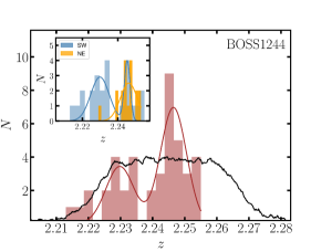
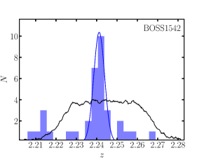
Figure 9: The redshift distributions of the confirmed HAEs in BOSS1244 (left) and BOSS1542 (right). The inner panel of left figure is the redshift distribution of HAEs in the BOSS1244 SW and NE regions. The black solid line is the transmission curve of the NB filter.

3.3 Overdensity and Present-day Masses Estimate

Galaxy overdensity $\delta_{\rm g}$ is estimated from the galaxy surface density, where $\delta_{\rm g}$ is defined as $\delta_{\rm g}=\frac{\Sigma_{\rm group}}{\Sigma_{\rm field}}-1$, $\Sigma_{\rm group}$ is the HAE number per arcmin² within the overdensity, and $\Sigma_{\rm field}$ is the surface density of HAEs in the random fields. Our NIR spectroscopically-confirmed HAEs indicate that BOSS1244 and BOSS1542 are indeed extremely overdense. The surface densities of HAE candidates at $z=2.24$ in the BOSS1244 and BOSS1542 fields are 0.585$\pm$0.037 and $0.559\pm 0.037$ HAE arcmin^-2, respectively. The surface density $\Sigma_{\rm field}$ of HAEs is calculated through some popular general fields with large HAE surveys. An et al. (2014) detected 28$\pm$5 HAE candidates at $z=2.24$ with the same narrowband, detection depth and selection criteria over 383 arcmin² area in ECDFS and the surface density $(7.31\pm 1.38)\times 10^{-2}$ HAE arcmin^-2. Sobral et al. (2013) performed a large H$\alpha$ survey at $z=2.23,1.47,0.84$ and 0.4 in the Cosmological Evolution Survey (COSMOS) and Ultra Deep Survey (UDS) fields. Using the same criteria of HAE candidates, the average surface densities in COSMOS and UDS are estimated to be $(8.25\pm 0.36)\times 10^{-2}$ and $(7.01\pm 0.53)\times 10^{-2}$ HAE arcmin^-2, respectively. Note that there is an overdense region in COSMOS so that the surface density is higher than that in ECDFS and UDS, which is reported in Geach et al. (2012). If the overdense region is masked, the surface density in COSMOS is $(7.42\pm 0.35)\times 10^{-2}$ HAE arcmin^-2. In addition, 11 HAE candidates at $z=2.19\pm 0.02$ over $\sim 70\,$arcmin² are reported in the Great Observatories Origins Deep Survey North (GOODS-N) field (Tadaki et al., 2011), the surface density is $0.157\pm 0.047$ HAE arcmin^-2, which is about twice as high as other general fields (like ECDFS, COSMOS and UDS). This is mainly due to the limited NB survey area (Tadaki et al., 2011). For a comparison, we expect $31\pm 6$ HAEs in our areas, based on integrating the H$\alpha$ luminosity function (Sobral et al., 2013) and the completeness function of HAEs. The surface density in random fields is $(7.43\pm 1.44)\times 10^{-2}$ HAE arcmin^-2. The method is described in Lee et al. (2014b). Here we adopt as the average surface density ($7.25\pm 0.51)\times 10^{-2}$ HAE arcmin^-2 of HAE candidates in the ECDFS, COSMOS and UDS fields for estimating HAE overdensities of the BOSS1244 and BOSS1542 fields.

We do not map out all the HAE candidates in our NIR spectroscopic observations. However, considering the fore- and back-ground emitter contaminations, we assume that 80% of our sample are true HAEs at $z=2.24\pm 0.02$ based on the detect rate from our NIR spectroscopic analyses, and the galaxy overdensities $\delta_{\rm g}$ in BOSS1244 and BOSS1542 are computed to be 5.5$\pm$0.7 and 5.2$\pm$0.6, respectively. The results are consistent with Zheng et al. (2021). These two overdensities are the most overdense fields currently known over the volumes of $\sim(40)^{3}$ cMpc³, and thus provide ideal laboratories to study galaxy properties in dense environments and the environmental dependence of galaxy mass assembly at the cosmic noon.

The characteristic size of a protocluster is $\sim 15$ cMpc (10.5 $h^{-1}$ cMpc), and the protocluster mass is typically calculated in a volume of (15 cMpc)³ (Steidel et al., 1998, 2005; Chiang et al., 2013; Stark et al., 2015; Muldrew et al., 2015). To compare with our two overdensities (protoclusters), we measure $\delta_{\rm g}$ in BOSS1244 and BOSS1542 over the typical protocluster scale (volume). Since the line-of-sight depth of our survey is 56.9 cMpc, we measure the overdensity in a circular area 8.7 cMpc in diameter, which corresponds to the volume of (15 cMpc)³. In BOSS1244, two density peaks regions (NE and SW area) are separated in space and redshift obviously. The number of HAEs within a diameter of 8.7 cMpc (5.4 arcmin) centered on the position $[\alpha,\delta]=[190.892,35.909]$ in the SW dense region is $40\pm 6$, corresponding to a surface density of 1.73$\pm$0.26, and $\delta_{\rm g}=22.9\pm 4.0$. The number of HAEs within a diameter of 8.7 cMpc centered on the position $[\alpha,\delta]=[191.074,36.079]$ in the NE dense region is $20\pm 4$, corresponding to surface density of 0.87$\pm$0.17, and $\delta_{\rm g}$ is 10.9$\pm$2.5, which is lower than that in the SW region. In BOSS1542, it shows a giant filament structure with $\sim 14\farcm 6$ ($\sim 23.4$ cMpc) along the South to North region. We further calculate that the $\delta_{\rm g}$ through an elliptical area with an axial ratio of $1/3$ centered on the position $[\alpha,\delta]=[235.682,38.954]$. The estimated $\delta_{\rm g}$ in the (15 cMpc)³ volume is 20.5$\pm$3.9. The uncertainties are estimated in the galaxy number counts within an overdense region by including poisson shot noise and cosmic variance (clustering effect) (Lee et al., 2014b; Cai et al., 2017a).

Table 2: Galaxy overdensities and present-day masses in BOSS1244 and BOSS1542.

Cluster	Redshift	Scale	$\delta_{\rm g}$	Present-day Mass
name	$<z>$	[cMpc]		[$10^{15}$ $M_{\sun}$]
BOSS1244a	2.24	39.4	7.1$\pm$0.8	10.70$\pm$0.80
BOSS1244b	2.24	39.4	5.5$\pm$0.7	8.90$\pm$0.70
BOSS1244 NE	2.246$\pm$0.001	15	10.9$\pm$2.5	0.83$\pm$0.11
BOSS1244 SW	2.230$\pm$0.002	15	22.9$\pm$4.9	1.59$\pm$0.20
BOSS1542c	2.24	38.8	6.7$\pm$0.7	9.80$\pm$0.70
BOSS1542d	2.24	38.8	5.2$\pm$0.6	8.20$\pm$0.60
BOSS1542 Filament	2.241$\pm$0.001	15	20.5$\pm$3.9	1.42$\pm$0.18

^aThe emission line galaxy overdensity in BOSS1244. ^bThe HAE overdensity in BOSS1244 assuming 80% sample are true HAEs. ^cThe emission line galaxy overdensity in BOSS1542. ^dThe HAE overdensity in BOSS1542 assuming 80% sample are true HAEs.

Galaxy formation models predict that galaxies inside large-scale overdensities should be older than those outside, because matter fluctuations inside overdensities are sitting on a large-scale pedestal and easier to collapse by crossing the threshold of $\delta_{\rm c}=1.69$. We estimate the total masses at $z\sim 0$ in our two overdensities using the galaxy overdensity factor and the appropriate volume based on the approach outlined by Steidel et al. (1998, 2005), although there are some uncertainties such as systematic and random errors from the assumption of spherical collapse model (Chiang et al., 2013; Overzier, 2016). The equation is given by:

$$\centering M_{z\rm=0}=\bar{\rho}V_{\rm true}(1+\delta_{\rm m})\@add@centering$$ (1)

where $\bar{\rho}$ is the the mean comoving matter density of the universe, which is equal to $\frac{3H_{\rm 0}^{2}}{8\pi G}\Omega_{\rm m}=4.1\times 10^{10}$ $M_{\sun}$ cMpc^-3, and $V_{\rm true}$ is the volume in real space that encloses the observed galaxy overdensity after correcting the effects of redshift-space distortions. So Equation 1 is equivalent to $M_{z=0}=[4.1\times 10^{10}\,M_{\sun}](1+\delta_{\rm m})[V_{\rm true}/$ cMpc³], and $V_{\rm true}=V_{\rm apparent}/C$. $V_{\rm apparent}$ is the observed comoving volume. The observed volume $V_{\rm apparent}$ is 60,964 cMpc³ and 58,332 cMpc³ in BOSS1244 and BOSS1542, respectively. Namely, $\sim 20\farcm 4\times 20\farcm 4$ region in BOSS1244 and $20\farcm 0\times 20\farcm 0$ region in BOSS1542 are covered on the plane of sky between $z=2.223-2.267$ (the sight of comoving distance is about 56.9 cMpc). The matter overdensity $\delta_{\rm m}$ is related to the galaxy overdensity by $1+b\delta_{\rm m}=C(1+\delta_{\rm g})$, where $b$ is the HAE bias factor. We take $b_{\rm HAE}=2.4_{-0.2}^{+0.1}$ from Geach et al. (2012) to be the HAE bias at $z=2.24$. $C$ is the correction factor which is an estimation of the effects of redshift-space distortions caused by peculiar velocities (Steidel et al., 1998), which is a function of matter overdensity $\delta_{\rm m}$ and redshift $z$. In the case of spherical collapse, the correction factor $C$ can be estimated using the expression of $C=1+f-f(1-\delta_{\rm m})^{\frac{1}{3}}$, where $f=\Omega_{\rm m}(z)^{4/7}$, which we take to be $f=0.96$ at $z=2.24$.

We obtain the correction factor $C=0.62\pm 0.03$ and matter overdensity $\delta_{\rm m}=1.69\pm 0.15$ in BOSS1244, while $C=0.64\pm 0.03$ and matter overdensity $\delta_{\rm m}=1.62\pm 0.14$ in BOSS1542. According to the theory of density perturbation, we use the approximation for spherical collapse from the equation 18 in Mo & White (1996) to the linear matter density $\delta_{\rm L}$. The linear overdensity $\delta_{\rm L}$ in BOSS1244 and BOSS1542 is 0.74 and 0.73. If it evolves to the redshift of $z=0$, the linear overdensities $\delta_{\rm L}$ in BOSS1244 and BOSS1542 are 2.17 and 2.14, respectively, which is exceeding the collapse threshold of $\delta_{\rm c}=1.69$. We thus expect the entire BOSS1244 and BOSS1542 overdensities to be virialized by $z=0$. Using the Equation 1, the total masses at $z=0$ in the overall BOSS1244 and BOSS1542 fields are $(0.89\pm 0.07)\times 10^{16}$ $M_{\sun}$ and $(0.82\pm 0.06)\times 10^{16}$ $M_{\sun}$, respectively. We find that the same volume without an overdensity $\delta_{\rm m}$ results in a mass of $(3.70\pm 0.18)\times 10^{15}$ $M_{\sun}$ in BOSS1244 and $(3.48\pm 0.16)\times 10^{15}$ $M_{\sun}$ in BOSS1542. Kurk et al. (2004b) explained that the masses may be mostly intergalactic gas which will disappear out of the cluster with the Hubble flow, and eventually evolve into the mass of the bound system, although they gave an error in computing the value of $\bar{\rho}V_{\rm true}$, being pointed out in Steidel et al. (2005).

Table 3: Dynamical properties in this work and other protoclusters at $z=2-3$.

Cluster	Redshift	$\sigma_{\rm los}$	$r_{200}$	$M_{200}$	Reference
name	$z$	[km s-1]	[Mpc]	[$10^{13}$ $M_{\sun}$]
SSA 22 Blue	3.069	350$\pm$53	$0.19\pm 0.03$	$1.6\pm 0.7$	Topping et al. (2016)
SSA 22 Red	3.095	540$\pm$40	$0.29\pm 0.02$	$5.9\pm 1.3$	Topping et al. (2016)
MRC 0943–242	2.92	715$\pm$105	$0.41\pm 0.06$	$15\pm 6$	Venemans et al. (2007)
MRC 0052–241	2.86	980 $\pm$120	$0.57\pm 0.07$	$38\pm 14$	Venemans et al. (2007)
USS 1558-003 C1	2.53	284	0.19	1.00	Shimakawa et al. (2014)
USS 1558-003 C2	2.53	574	0.38	8.70	Shimakawa et al. (2014)
CL J1001	2.506	530$\pm$120	0.36$\pm$0.08	7.94$\pm$3.80	Wang et al. (2016)
PCL1002	2.47	426	$0.29$	$3.7$	Casey et al. (2015)
PKS 1138-262	2.16	683	0.53	17.10	Shimakawa et al. (2014)
BOSS1441	2.32	943$\pm$500	0.7$\pm$0.4	40.0${}_{-39}^{+70}$	Cai et al. (2017a)
CC2.2	2.23	645$\pm$69	0.49$\pm$0.05	14.0$\pm$5.0	Darvish et al. (2020)
BOSS1244 NE	2.246	377$\pm$99	0.28$\pm$0.07	2.80$\pm$2.20	This work
BOSS1244 SW	2.230	405$\pm$202	0.30$\pm$0.15	3.00$\pm$5.00	This work
BOSS1542 Filament	2.241	247$\pm$32	0.19$\pm$0.02	0.79$\pm$0.31	This work

The progenitors of galaxy clusters at $z\sim 0$ have a characteristic size of 15 cMpc, we thus estimate the total present-day masses of the density peak structures in the volume of (15 cMpc)³. The density peak regions in BOSS1244 and BOSS1542 are expected to be virialized at $z\sim 0$. As described in Section 3.2, BOSS1244 has two different components: the NE region with $\delta_{\rm g}=10.9\pm 2.5$ and SW region with $\delta_{\rm g}=22.9\pm 4.0$ over the 15 cMpc scale. Using the Equation 1, the total masses at $z=0$ in NE and SW are expected to be $(0.83\pm 0.11)\times 10^{15}$ $M_{\sun}$ and $(1.59\pm 0.20)\times 10^{15}$ $M_{\sun}$, respectively. The mass in SW is about twice the mass in NE, which is related to the HAE overdensity. In contrast, BOSS1542 displays a huge filamentary structure and $\delta_{\rm g}$ is $20.5\pm 3.9$ over the 15 cMpc scale at $z=2.241$, and the present-day mass is $(1.42\pm 0.18)\times 10^{15}$ $M_{\sun}$. We summarize $\delta_{\rm g}$ and present-day masses of the BOSS1244 and BOSS1542 fields in Table 2.

Furthermore, we estimate the total enclosed mass from the scaling relation based on cosmological simulation. Chiang et al. (2013) presented the correlation between mass overdensity $\delta_{\rm m}$ at different redshifts and the descendant cluster mass $M_{z=0}$ in the (13.1 cMpc)³ and (24.1 cMpc)³ tophat box windows. We thus estimate $M_{z=0}$ based on our calculated matter overdensity in the same volume. Using $b=2.4$ as above, in the volume of (13.1 cMpc)³, the matter overdensity $\delta_{\rm m}$ in BOSS1244 SW and NE regions is $12.6\pm 2.5$ and $5.6\pm 1.6$, respectively, and $\delta_{\rm m}$ in BOSS1542 is $9.3\pm 2.1$. According to the correlation between overdensity and present-day total mass, we estimate the descendant cluster masses $M_{z=0}$ are $>2\times 10^{15}$ $M_{\sun}$ in BOSS1244 SW region and in $(1.24\pm 0.24)\times 10^{15}$ $M_{\sun}$ NE region, and $M_{z=0}$ in BOSS1542 is $>2\times 10^{15}$ $M_{\sun}$. By comparison of the method of Steidel et al. (1998), we find that mass estimation presented by Chiang et al. (2013) is about twice as high as the method in Steidel et al. (1998), but both mass estimates suggest that BOSS1244 and BOSS1542 protoclusters over the 15 cMpc scale will evolve into Coma-type ($\geq 10^{15}$ $M_{\sun}$) clusters in the present epoch.

3.4 Velocity Dispersions of Two Overdensities

As described in 3.2, BOSS1244 shows two distinct spikes at $z=2.230$ in the SW region and $z=2.246$ in the NE region, and the SW region appears to be much denser than that the NE region. The line-of-sight depth between $z=2.230$ and $z=2.246$ is 21 cMpc. In both regions, we estimate the line-of-sight velocity dispersion from our measured spectroscopic redshifts using two Gaussian functions. The velocity dispersion in the SW region is $405\pm 202$ km s^-1, similar to the velocity dispersion in the NE region ($377\pm 99$ km s^-1). SW region in BOSS1244 also presents two substructures in redshift distribution (the left inner panel of Figure 9) and the velocity dispersions of these two substructures are $484\pm 181$ km s^-1 at $z=2.230$ and $152\pm 58$ km s^-1 at $z=2.245$. The lower velocity dispersion infers that the structure might perpendicular to the line-of-sight (Venemans et al., 2007), or might be due to the smaller number HAEs that we estimate the velocity dispersion. For BOSS1542, our NIR spectroscopic observations present an extended and narrow filamentary structure on the scale of 23.4 cMpc (the right panel of Figure 9). The estimated velocity dispersion is $247\pm 32$ km s^-1 at $z=2.241$, which is much lower than that in BOSS1244. The lower velocity dispersion may indicate that BOSS1542 is a dynamically young protocluster (Dey et al., 2016).

We also use the bi-weight method to check the line-of-sight velocity dispersion from the measured spectroscopic redshifts considering that this method is shown to be robust against a few outliers and for non-Gaussian underlying distributions (Beers et al., 1990). The velocity dispersions of NE and SW regions are $320\pm 60$ km s^-1 at $z=2.247$ and $431\pm 99$ km s^-1 at $z=2.231$, respectively. The velocity dispersions of two components in the SW region are $304\pm 99$ km s^-1 at $z=2.246$ and $430\pm 119$ km s^-1 at $z=2.230$. The velocity dispersion in the BOSS1542 filament within 2$\sigma$ is $255\pm 48$ km s^-1 at $z=2.241$. All these estimates are consistent with the results obtained with the Gaussian methods. We adopt the measured results using the Gaussian method hereafter.

3.5 Dynamical Mass

Protocluster systems are not virialized, and the velocity dispersion of member galaxies traces the dynamical state of system rather than the halo mass (Wang et al., 2016; Darvish et al., 2020). Still, dynamical mass estimates provide upper limits for the actual masses, given that the galaxies most likely populate multiple halos within the protocluster system rather than one virialized system (Lemaux et al., 2014; Dey et al., 2016; Overzier, 2016). We apply the method for virialized systems to our protoclusters to draw an upper limit of dynamical mass and examine their dynamical state.

We first assume that BOSS1244 and BOSS1542 protoclusters at $z=2.24$ are virialized and the halos of the two protoclusters are spherical region within which the average density is $200\,\rho_{\rm c}(z)$. The virial mass $M_{200}=\frac{4\pi}{3}r_{200}^{3}200\rho_{\rm c}(z)$, where $r_{\rm 200}$ is the virial radius and $\rho_{\rm c}(z)=3H^{2}(z)/(8\pi G)$ is the critical density of the universe at redshift of $z$. Using a spherical symmetry combined with the virial theorem and the line-of-sight velocity dispersion $\sigma_{\rm los}$, the virial radius is $r_{200}=GM_{200}/(3\sigma_{\rm los}^{2})$, where $G$ is the gravitational constant. Using above three formulae, we can derive $r_{200}$ and $M_{200}$ as a function of $\sigma_{\rm los}$ and $H(z)$: $M_{200}=(\sqrt{3}\sigma_{\rm los})^{3}/(10GH(z))$ and $r_{200}=\sqrt{3}\sigma_{\rm los}/(10H(z))$. For BOSS1542 protocluster, we estimate virial radius $r_{200}=0.19\pm 0.02$ Mpc and virial mass $M_{200}=(0.79\pm 0.31)\times 10^{13}$ $M_{\sun}$. For BOSS1244 protocluster, we estimate $r_{200}=0.28\pm 0.07$ Mpc and $M_{200}=(2.80\pm 2.20)\times 10^{13}$ $M_{\sun}$ in the NE region, and $r_{200}=0.30\pm 0.15$ Mpc and $M_{200}=(3.00\pm 5.00)\times 10^{13}$ $M_{\sun}$ are computed in the SW region. The large errors in mass are due to the relatively large velocity dispersion errors.

We also use the scaling relation between velocity dispersion and total mass presented in Evrard et al. (2008) to estimate the dynamical total masses.

$$\centering\sigma_{\rm DM}(M,z)=\sigma_{\rm DM,15}\left[\frac{h(z)M_{200}}{10^{15}M_{\odot}}\right]^{\alpha}\@add@centering$$ (2)

where $\sigma_{\rm DM,15}$ is normalization at mass $10^{15}\,M_{\odot}$ and $\alpha$ is the logarithmic slope. Using $\sigma_{\rm DM,15}=1082.9\pm 4.0$ km s^-1 and $\alpha=0.3361\pm 0.0026$, we can derive the halo masses in our protoclusters (see also Munari et al., 2013). The virial masses $M_{200}$ in the BOSS1244 NE region, BOSS1244 SW region and BOSS1542 filament are $(1.90\pm 1.50)\times 10^{13}$ $M_{\sun}$, $(2.30\pm 3.50)\times 10^{13}$ $M_{\sun}$ and $(5.30\pm 2.10)\times 10^{12}$ $M_{\sun}$, respectively. The derived $M_{200}$ using the scaling relation is consistent with our estimate based on the virial theorem.

We find that the dynamical masses of two substructures in BOSS1244 are $\sim 2-3$ times that of BOSS1542, indicating that they may be in different dynamic evolution states. Wang et al. (2016) discovered an X-ray detected galaxy cluster with a halo of $M_{200}\sim 10^{13.7\pm 0.2}$ $M_{\sun}$ based on the velocity dispersion of $530\pm 120\,$km s^-1 at $z=2.506$. Shimakawa et al. (2014) presented two protoclusters PKS 1138-262 at $z=2.16$ and USS 1558-003 at $z=2.53$, and the dynamical mass of the core is estimated to be $M_{200}=1.71\times 10^{14}$ $M_{\sun}$with the velocity dispersion of $683\,$km s^-1 and $M_{200}=0.87\times 10^{14}$ $M_{\sun}$ with the velocity dispersion of $574\,$km s^-1, respectively. Recently, Darvish et al. (2020) showed a new protocluster CC2.2 in COSMOS at $z=2.23$. The redshift and selection technique of HAEs are the same as ours used for BOSS1244 and BOSS1542. The dynamical mass of CC2.2 is $M_{200}=(1.40\pm 0.5)\times 10^{14}$ $M_{\sun}$ and the velocity dispersion is $645\pm 69\,$km s^-1. They are summarized in Table 3. These protocluster systems will evolve into fully collapsed and virialized Coma-type structures with a total mass of $M_{200}\sim 10^{15}$ $M_{\sun}$ at $z=0$, so they are likely to be in transition phase between protoclusters and mature clusters. However, the dynamical masses in the BOSS1244 and BOSS1542 protoclusters are $\sim 1-2$ order-of-magnitude lower than that in above mentioned protoclusters, suggesting that BOSS1244 and BOSS1542 protoclusters are pre-virialized, younger systems. This provides evidence on earlier phase during which the clusters and their members are actually forming.

4 Discussions

4.1 CoSLAs and Quasar Pairs in the Two Overdensities

Protoclusters are not only traced by overdensities of galaxies, but also by intergalactic hydrogen gas that can produce Ly$\alpha$ absorption in the spectra of background quasars. Four out of five background quasars at $2.3<z<3.2$ in BOSS1244/BOSS1542 are used to measure the Ly$\alpha$ absorption. These background quasars $2-30$ cMpc away from the center of two fields in sky projection, with the effective optical depths of IGM absorption of $3-5\times$ the average optical depth ($\sim$0.25) at $z=2.24$. We find that no CoSLAs are in the dense region in BOSS1244, and all of them are distributed in the periphery of the BOSS1244 field. In contrast, two CoSLAs are located in the BOSS1542 filamentary structure and others are in the outskirts of the BOSS1542 field.

In BOSS1244, we note that the background quasar marked “1” is located between SW and NE regions and is $\sim 6.85\,$cMpc away from the field center. The line-of-sight distance between SW and NE region and the CoSLAs at $z=2.24$ detected by background quasar is $7.8\,$cMpc and $13.0\,$cMpc, respectively. From the upper left of the figure 1 of Zheng et al. (2021), we find that this CoSLA shows a double peak in the line-of-sight distance with $>3\times$ the average optical depth, corresponding to the comoving distance of $0-10\,$cMpc and $10-20\,$cMpc. It confirms that BOSS1244 should consists of two separated components along the line-of-sight direction, which is consistent with our spectroscopic observations. The background quasar marked “2” is around the SW region with the line-of-sight distance of $10-20\,$cMpc, the background quasars marked “3” and “4” are around the NE region with the line-of-sight distance of $0-10\,$cMpc. Similarly, BOSS1542 also shows the consistent results from the effective optical depth profile described in the figure 2 of Zheng et al. (2021). In short, these reflect the importance of NIR spectroscopic observations and indicate that the redshift we measured is reliable.

Furthermore, there are five BOSS quasars at $z=2.23-2.26$ in BOSS1244 and three BOSS quasars at $z=2.23-2.25$ in BOSS1542, as shown in Table 4. We find that the measured redshifts of the HAEs are consistent with the redshifts of these quasars around them, and most of these BOSS quasars are in the overdense regions of BOSS1244 and BOSS1542, indicating that these quasars are likely to be associated with the two overdensities. In BOSS1244, we find that QSO2/QSO5 with projected separation $\sim 1.2$ pMpc and velocity offset $\sim 1570$ km s^-1 meets the definition of quasar pairs with a projected separation $<2(=1.4h^{-1}$) pMpc and velocity offset $<2300$ km s^-1 (Onoue et al., 2018). In BOSS1542, QSO2/QSO3 with projected separation $\sim 1.9$ pMpc and velocity offset $\sim 740$ km s^-1 is a quasar pair. Interestingly, the quasar pairs QSO2/QSO5 in BOSS1244 and QSO2/QSO3 in BOSS1542 are located in the overdense region, suggesting that the overdensities of galaxy are associated with quasar pairs. Some works show that quasar pair environment has a systematic larger overdensity of galaxies around quasars in pairs with respect to that of isolated quasars at $z<1.0$ (Farina et al., 2011; Hennawi et al., 2015; Sandrinelli et al., 2018; Onoue et al., 2018). However, some works suggest no enhancement in the galaxy density around the quasar pair at low-$z$ or high-$z$ (Green et al., 2011; Sandrinelli et al., 2014; Fukugita et al., 2004). Onoue et al. (2018) pointed out that pairs of luminous quasars at $z>3$ and $z\sim 1.0$ are better tracers of protoclusters than single quasars, but are not tracing the most overdense protoclusters. In Cai et al. (2017a), we find that the first MAMMOTH overdensity BOSS1441 has two quasar pairs with the projected separations are $\sim 1.8$ pMpc/$2.0$ pMpc and the velocity offsets are $\sim 900$ km s^-1/$100$ km s^-1, which also reside in the density peak of the overdensity. Therefore, these observations provide further evidence that overdensity of galaxy at $z=2-3$ could also be traced by the quasar pairs.

Table 4: BOSS QSOs (including background QSOs) in the BOSS1244 and BOSS1542 fields.

Field	ID	R.A.	Decl.	Redshift
		(J2000.0)	(J2000.0)	$z$
	BG QSO1	191.11745	36.122048	3.212
	BG QSO2	190.70921	35.966921	3.143
	BG QSO3	190.81858	36.145731	2.888
	BG QSO4	191.08365	36.151788	2.863
BOSS1244	BG QSO5	190.90702	36.031874	2.437
	QSO1 (HAE)	191.10603	36.132581	2.260
	QSO2 (HAE)	190.91308	35.901003	2.245
	QSO3 (HAE)	191.01176	35.935079	2.235
	QSO4 (HAE)	191.11257	36.152239	2.233
	QSO5 (HAE)	190.90429	35.941498	2.228
	BG QSO1	235.47301	38.774797	2.781
	BG QSO2	235.43314	39.149935	2.717
	BG QSO3	235.72489	38.834426	2.477
	BG QSO4	235.63317	39.148571	2.356
BOSS1542	BG QSO5	235.66231	38.913783	2.267
	QSO1 (HAE)	235.62312	39.021790	2.250
	QSO2 (HAE)	235.70368	38.960585	2.242
	QSO3 (HAE)	235.69590	38.895094	2.234

4.2 Internal Structures

Kinematical structures of distant protoclusters provide essential information on the mass assembly history of galaxy clusters. Figure 10 and Figure 11 show the three-dimensional spatial distribution of HAEs in BOSS1244 and BOSS1542, the color-coded filled points are the confirmed HAEs with NIR spectroscopy. In terms of the large-scale geometry, the BOSS1244 and BOSS1542 protoclusters are very different, suggesting that they are in different stages of evolution.

4.2.1 BOSS1244 with multiple components

BOSS1244 shows two distinct components (NE and SW) both in space and in redshift distribution, and two substructures in the SW region. The redshift difference between SW and NE regions is $\Delta z=0.016$ (the line-of-sight depth is 20.8 cMpc), and the projected separation between them is 13$\farcm$5 ($\sim 21.6$ cMpc). The right panel in Figure 10 is the spectroscopic confirmed HAEs, we find that serveral substructures are in the SW and NE regions. In the SW region, there are about five subgroups with $\geq 3-5$ galaxies at $2.213<z<2.221$, $2.224<z<2.229$, $2.234<z<2.236$, $2.242<z<2.247$ and $2.248<z<2.257$. There are two subgroups with $\geq 5$ galaxies in the NE region at $2.238<z<2.245$ and $2.246<z<2.255$. These subgroups are clustered together along the line-of-sight direction. The hierarchical structure formation model predicts that the larger structures are formed from smaller substructures through the continuous merging (e.g., Kauffmann & White, 1993; Kauffmann et al., 1999). The subgroups in SW and NE regions might continue to grow into larger structures.

We want to know whether the SW and NE protoclusters can collapse to a single rich cluster, or evolve into two independent massive halos as parts of a supercluster. A typical size of the effective radius is $\sim$3.2 cMpc at $z\sim 2.2$ for the progenitors of $(1-3)\times 10^{14}$ $M_{\sun}$ halos at $z=0$ and the size is about 6.5 cMpc for those of $>10^{15}$ $M_{\sun}$(Chiang et al., 2013). According to theoretical simulations, Muldrew et al. (2015) predicted that the average radius of protoclusters is $\sim 9-13\,$cMpc at $z\sim 2$ for the descendants of $(4-10)\times 10^{14}$ $M_{\sun}$ halos. The main protoclusters and their surrounding groups/clusters could merge into a single galaxy cluster by $z=0$ only if a descendant halo mass at $z=0$ is $>10^{15}$ $M_{\sun}$ (Muldrew et al., 2015). The present-day total mass in SW component is $(1.59\pm 0.20)\times 10^{15}$ $M_{\sun}$, which is twice that of the NE component. It is possible that the NE component falls to the larger SW component through the gravitational potential well, and merge to a larger structure eventually.

For what concerns merger events, Lee et al. (2016) reconstructed a 3D tomographic map of the foreground Ly$\alpha$ forest absorption at $z=2-3$ using the background LBGs and quasars in COSMOS. Using mock tomographic maps, they found that very few of protoclusters with an elongated shape will collapse to one single cluster at $z\sim 0$. The proto-supercluster was identified with seven density peaks subsequently (Cucciati et al., 2018). Topping et al. (2018) presented the Small MultiDark Planck Simulation on searching for the $z\sim 3$ protoclusters with a double peak in redshift distribution and the two peaks separated by 2000 km s^-1, like SSA22 protocluster (Topping et al., 2016). They found that such double-peaked overdensities are not going to merge into a single cluster at $z=0$. The redshift separation between SW and NE protoclusters in BOSS1244 is 0.016, and the velocity offset is $\sim 1486\,$km s^-1. Their projected separation is $\sim$21.6 cMpc, which is much larger than the typical size of protoclusters. The BOSS1244 structure is similar to the SSA22 protocluster, so it may evolve into two separated clusters at $z\sim 0$.

In the local universe ($z<0.5$), superclusters are typically a few cMpc to $\sim$100 cMpc in size (Rosati et al., 1999; Kim et al., 2016), with wide ranges of mass from a few $10^{14}$ $M_{\sun}$ to $10^{16}$ $M_{\sun}$ (Swinbank et al., 2007; Bagchi et al., 2017), and most of superclusters are composed of two or three galaxy clusters, and a few of them include nearly 10 clusters (Lubin et al., 2000; Lemaux et al., 2012). Figure 10 displays the three-dimensional distribution (sky and redshift positions) of our spectroscopically-identified protocluster galaxies in BOSS1244. We find that there are many smaller components and they may be forming large-scale structures, and the present-day total mass in the whole system is $\sim 10^{16}$ $M_{\sun}$. It suggests that BOSS1244 may also be evolved into a supercluster with two massive galaxy clusters at $z\sim 0$.

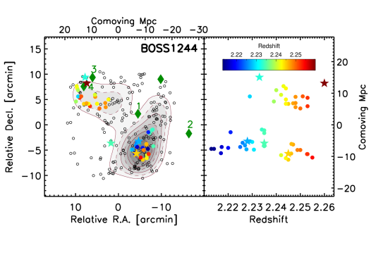
Figure 10: Three-dimensional distribution of the protocluster galaxies in the BOSS1244 field. Sky coordinates are listed relative to the centre of the BOSS1244 field. The color-coded points and stars are the confirmed HAEs and quasars at $z=2.213-2.260$. Left: HAEs plotted as Decl. vs. R.A. The black circles are the HAE candidates in BOSS1244. Right: Confirmed HAEs plotted Decl. vs. $z$. There is a separation in the distributions of galaxies both in Decl. and $z$.

4.2.2 BOSS1542 with an extended filamentary structure

Filaments are ubiquitous in the universe and and account for $\sim 40-60\%$ of the matter in the universe, but only $\sim 6-16\%$ of the volume (Tempel et al., 2014; Martizzi et al., 2019). Cosmic filaments are elongated relatively high density structures of matter, tens of Mpc in length, and intersect at the location of galaxy clusters. They form through a gravitational collapse of matter driven by gravity (Codis et al., 2012; Laigle et al., 2015; Kraljic et al., 2018; Kuchner et al., 2020). BOSS1542 shows an enormous H$\alpha$ filamentary structure with a projected length of 23.4 cMpc running in the North-South direction, shown in Figure 11. The galaxy overdensities $\delta_{\rm g}$ in the filament region over a typical protocluster scale (15 cMpc) is $20.5\pm 3.9$, corresponding to the present-day halo mass of $(1.42\pm 0.18)\times 10^{15}$ $M_{\sun}$. It indicates that the H$\alpha$ filament structure in BOSS1542 will evolve into a Coma-type galaxy cluster at $z\sim 0$.

Recently, Umehata et al. (2019) presented a cold-gas filament of the cosmic web in Ly$\alpha$ emission in the core of the SSA22 protocluster at $z=3.09$. The network of filaments in SSA22 is found to connect individual galaxies across a large volume, allowing it to power star formation and black hole growth in active galaxy populations at $z\sim 3$. It is suggested that similar structures may be a general feature of protoclusters in the early universe (Martin et al., 2014; Kikuta et al., 2019). In BOSS1542, we find that star-forming galaxies (HAEs), quasars and CoSLAs detected by background quasars reside in this filamentary, the velocity dispersion of this structure is $247\pm 32\,$km s^-1, suggesting that it is a dynamically young structure. Cosmological simulations of structure formation predict that the majority of gas in the intergalactic medium (IGM) is distributed in a cosmic web of sheets and filaments by gravitational collapse (Bond et al., 1996). The cold gas is falling along the filaments driven by gravity and the filaments are able to provide most of the gas required for the growth of galaxies and SMBHs. Using absorption spectroscopy of background sources to trace neutral hydrogen in the IGM, which will provide insights into the nature of the cosmic web. The filament in BOSS1542 is providing a direct detection of the cosmic web in the early universe. In the future, we will search for LAEs, LABs, X-ray luminous AGNs and SMGs in the BOSS1542 filamentary structure to understand how the universe evolved through time, how galaxies grow and mature, and how the changing environments affect galaxy properties at $z=2-3$.

From the right panel of Figure 11, our NIR spectroscopic observations show that BOSS1542 is dominated by one component with an extended filament at $2.235<z<2.245$. However, at the intersection of this filamentary structure, several substructures without NIR spectroscopy confirmation are gathering together. For these regions, we need much more NIR spectroscopy to reveal their dynamical nature. Similarly, given the total mass of $\sim 10^{16}$ $M_{\sun}$ at $z\sim 0$, BOSS1542 may also evolve into a supercluster in the late time.

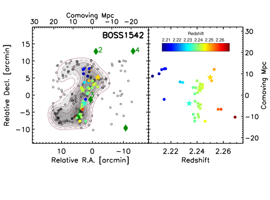
Figure 11: Three-dimensional distribution of the protocluster galaxies in the BOSS1542 field. Sky coordinates are listed relative to the centre of the BOSS1542 field. The color-coded points and stars are the confirmed HAEs and quasars at $z=2.206-2.269$. Left: HAEs plotted as Decl. vs. R.A. The black circles are the HAE candidates in BOSS1244. Right: Confirmed HAEs plotted Decl. vs. $z$. There is no significant difference in the distributions of galaxies in Decl.

4.2.3 Comparison with other protoclusters at $z>2$

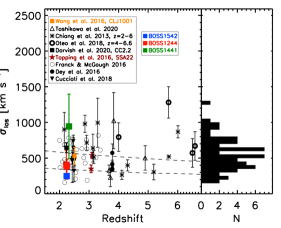
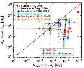
Figure 12: Left panel: velocity dispersion of protoclusters as a function of redshift and the histogram of the velocity dispersion of protoclusters. The red squares are the SW and NE protoclusters in BOSS1244, the blue square is the protocluster in BOSS1542, and other black symbols are the other protoclusters from the literature (Chiang et al., 2013; Lemaux et al., 2014; Dey et al., 2016; Wang et al., 2016; Franck & McGaugh, 2016; Topping et al., 2016; Cai et al., 2017a; Cucciati et al., 2014, 2018; Oteo et al., 2018; Toshikawa et al., 2020; Darvish et al., 2020; Hill et al., 2020). The dashed lines show the redshift evolution of dark matter velocity dispersion of $1\times 10^{14}$ $M_{\sun}$ and $5\times 10^{14}$ $M_{\sun}$ halos at $z=0$, which is from Toshikawa et al. (2020). Right panel: virial mass $M_{\rm vir}$ derived from velocity dispersion, vs. the present-day total mass $M_{\rm tot}$ estimated from galaxy overdensity. The red squares are the SW and NE protoclusters in BOSS1244 and the blue square is the protocluster in BOSS1542. The rightmost red square is our estimated velocity dispersion of the entire BOSS1244 system. Other symbols are the other protoclusters from the literature (Cucciati et al., 2014; Lemaux et al., 2014; Franck & McGaugh, 2016; Cai et al., 2017a; Topping et al., 2016, 2018; Cucciati et al., 2018; Darvish et al., 2020). The dot-dashed line shows the 1:1 relation between $M_{\rm vir}$ and $M_{\rm tot}$.

We compare other protoclusters at $z=2-3$ from literature with our protoclusters. The protoclusters reported in the literature has a median present-day halo masses of log$(M/M_{\sun})_{z=0}=14.6$ (Overzier, 2016). Not only will our entire overdensities ($\sim 10^{16}$ $M_{\sun}$) be among the most massive clusters known today, but the density peaks ($\delta_{\rm g}>20$) will be evolved into massive galaxy clusters of $>10^{15}$ $M_{\sun}$ at $z=0$.

Lemaux et al. (2014) discovered a massive protocluster (Cl J0227-0421) at $z=3.29$ with a galaxy overdensity of $10.5\pm 2.8$. They estimated the dynamical mass of $\sim 3\times 10^{14}$ $M_{\sun}$, and expected a halo mass of $\sim(3.67-8.69)\times 10^{15}$ $M_{\sun}$ for the $z=0$ cluster. Cucciati et al. (2018) presented a proto-supercluster at $z=2.45$ by identifying seven galaxy groups within a volume of $\sim 60\times 60\times 150\,$cMpc³. The total mass in each galaxy group at $z=0$ is about $9.2\times 10^{12}-2.6\times 10^{14}$ $M_{\sun}$, and the estimated present-day mass in the effective volume of $9.5\times 10^{4}\,$cMpc³ is $\sim 4.8\times 10^{15}$ $M_{\sun}$. The effective volume of the proto-supercluster is slightly larger than that in our protoclusters ($6.2\times 10^{4}\,$cMpc³), but estimated present-day mass is $2-3$ times less than ours. The main reason is that the estimation of mass depends not only on volume, but also on the galaxy overdensity. Topping et al. (2018) investigated the nature of large-scale structure in the SSA22 protocluster region at $z=3.09$ with a galaxy overdensity of $7.6\pm 1.4$. The expected total halo mass at $z=0$ is $(3.19\pm 0.40)\times 10^{15}$ $M_{\sun}$ over a volume of $\sim 12\times 14\times 43\,$cMpc³. They revealed two separated overdensities at $z=3.065$ and $z=3.095$, corresponding to the present-day masses are $(0.76\pm 0.17)\times 10^{15}$ $M_{\sun}$ and $(2.15\pm 0.32)\times 10^{15}$ $M_{\sun}$, respectively. Our findings of the large-scale structures in BOSS1244 seem to exhibit a consistent size and number of components with similar present-day masses. Recently, Darvish et al. (2020) reported a protocluster (CC2.2) in the COSMOS field at $z=2.23$ traced by the spectroscopic confirmation of HAEs. The galaxy overdensity is $\sim 6.6$ over the volume of $\sim 5500$ cMpc³, corresponding to the halo mass of $\sim 9.20\times 10^{14}$ $M_{\sun}$ at $z=0$. The dynamical mass is $\sim(1-2)\times 10^{14}$ $M_{\sun}$, suggesting the CC2.2 protocluster is not fully virialized at $z=2.23$. Similarly, our protoclusters are also identified by the NIR spectroscopy of HAEs at the same redshift, suggesting that our protocluster system are dynamically younger and in the process of galaxy accretion and merging, which are far from virialization, especially for the BOSS1542 protocluster. The NE protocluster in BOSS1244 is similar to the CC2.2 protocluster given their consistent galaxy overdensities and expected halo masses at $z=0$.

Cai et al. (2017a) reported the first MAMMOTH protocluster BOSS1441 at $z=2.32$. This protocluster contains a dominant dark matter halo that would likely collapse into a virialized cluster with mass $M_{z=0}=10^{15}$ $M_{\sun}$. For BOSS1441, BOSS1244 and BOSS1542, the three overdensities selected from the same technique display dramatically different in morphology, representing different stages of galaxy cluster assembly. We suspect BOSS1441 is a nearly-virialized protocluster, BOSS1244 is forming one or two protoclusters, and BOSS1542 is forming a filamentary structure. These processes are also expected in the cosmological simulations (Shandarin & Zeldovich, 1989; van de Weygaert & Bond, 2008; Shandarin & Sunyaev, 2009; Libeskind et al., 2018). Namely, considering a non-spherical collapse of an ellipsoildal overdensity for the real perturbations, the expansion turns into collapse along shortest axis first to form a “pancake” sheet structure, then along the intermediate axis to form filaments, and only at the end to fully collapse along the longest axis to form clusters (e.g., Libeskind et al., 2018).

For the rarity of these two structures, Cai et al. (2017a) found 11 fields at $z=2-3$ that contain groups of strong IGM Ly$\alpha$ absorption over the volume of $10^{8}\,$cMpc³, but 30% of the 11 absorptions have $>10^{15}$ $M_{\sun}$, where BOSS1441, BOSS1244 and BOSS1542 are included and identified. Namely, the volume density of high-mass of $>10^{15}$ $M_{\sun}$ is $\sim 3\times 10^{-8}\,$cMpc^-3. However, BOSS1244 and BOSS1542 have currently the highest galaxy overdensities over the volume of $\sim(39\,\rm cMpc)^{3}$, corresponding to the present-day total masses of $\sim 10^{16}$ $M_{\sun}$, so the occurrence rate of such structures is expected to be $2\times 10^{-8}\,$cMpc^-3 at $z=2.2$. Darvish et al. (2020) detected one protocluster (CC2.2) at $z=2.23$ in the COSMOS field over the volume of $\sim 5.48\times 10^{5}\,$cMpc^-3 and the corresponding volume density is $1.8\times 10^{-6}\,$cMpc^-3, which is higher than our result. This reason is due to their limited effective volume. According to simulations, Topping et al. (2018) found that the presence of two massive halos separated by 2000 km s^-1 around the SSA22 protocluster is 7.4 Gpc^-3 at $z\sim 3$. The BOSS1244 with two massive protoclusters separated by 1500 km s^-1 is similar to the SSA22 protocluster, and their occurrence rate of such a structure is consistent.

4.3 Velocity Structure

BOSS1244 and BOSS1542 are the most massive structures consisting of multiple components. BOSS1244 has two distinct protoclusters in the SW and NE regions, the velocity dispersions are $405\pm 202\,$km s^-1 and $377\pm 99\,$km s^-1, respectively. Furthermore, the SW protocluster in BOSS1244 appears to be two components with the velocity dispersions of $484\pm 181$ km s^-1 and $152\pm 58$ km s^-1. In contrast, the estimated velocity dispersion in BOSS1542 filament is $247\pm 32$ km s^-1. Note that we do not map all the HAEs in BOSS1244 and BOSS1542 due to the limited NIR spectroscopic observations.

The line-of-sight velocity dispersions of density peaks in BOSS1244 and BOSS1542 are relatively small compared with those of studied protoclusters in the literature. For example, The velocity dispersions of the proto-supercluster with seven density peaks at $z=2.45$ are $320-737\,$km s^-1 (Cucciati et al., 2018). Venemans et al. (2007) discovered six protoclusters around eight radio galaxies at $z=2.0-5.2$, the velocity dispersions for these clusters were measured to be ranging from $\sim 250$ km s^-1 to 1000 km s^-1. In that sample, MRC 1138-262 (PKS 1138-262) at $z=2.16$ and MRC 0052-241 at $z=2.86$ protoclusters showed bimodal redshift distributions: MRC 1138-262 had double peaks with velocity dispersions of 280 km s^-1 and 520 km s^-1, and MRC 0052-241 had double peaks with velocity dispersions of 185 km s^-1 and 230 km s^-1. The best-studied system SSA22 protocluster (similar to the BOSS1244 protocluster) at $z=3.09$ showed two substructures with velocity dispersions of 350 km s^-1 and 540 km s^-1 (Topping et al., 2016). Using NIR spectroscopy of HAE sample, Darvish et al. (2020) estimated that the velocity dispersion of protocluster CC2.2 at $z=2.23$ is 645 km s^-1, which is higher than the velocity dispersions of our protoclusters. We calculate the velocity dispersion of BOSS1441 protocluster at $z=2.32$ from 18 Ly$\alpha$ spectroscopy is 943 km s^-1 (Cai et al., 2017a). It indicates that all these protoclusters may be in different dynamical state. The velocity dispersions of other known protocluster candidates at $z>2$ have been compiled (Kuiper et al., 2011; Cucciati et al., 2014; Toshikawa et al., 2014; Wang et al., 2016; Lemaux et al., 2014, 2018; Miller et al., 2018; Chanchaiworawit et al., 2019) in Figure 12. The left panel of Figure 12 presents a relationship between velocity dispersion and redshift of protoclusters. No significant correlation is seen between velocity dispersion and redshift, although the velocity dispersion is expected to increase with protocluster growth. Most protoclusters have velocity dispersions of $<600$ km s^-1, but some protoclusters show higher velocity dispersions, even $>1000$ km s^-1. We estimate the velocity dispersion for the whole BOSS1244 field is $1670\pm 963$ km s^-1 using the Gaussian fitting. We also apply the biweight method and estimate the velocity dispersion to be $1058\pm 142$ km s^-1, consistent with previous mentioned. Previous works explain that the protoclusters with higher velocity dispersions are in merging processes and forming more massive structures, and their dynamical state may be far from virialization (e.g., Dey et al., 2016; Toshikawa et al., 2020).

The right panel of Figure 12 presents dynamical masses based on the estimation of velocity dispersion as a function of present-day masses based on the Equation 1. The dot-dashed line lies on the 1:1 relation. Cucciati et al. (2018) presented a “Hyperion” proto-supercluster with seven density peaks, the estimated two sets of masses are surprisingly consistent with the agreement of $<2\sigma$. Moreover, one of the seven peaks (orange square in Figure 12) has already been identified as a virialized structure (Wang et al., 2016), but they suggested $M_{\rm total}$ may be underestimated given the most distant in reconstruction from the 1:1 relation between $M_{\rm total}$ and $M_{\rm vir}$. The evolution of a density fluctuation from the beginning of collapse to virialization can take a few gigayears. Furthermore, galaxies outside the peaks’ volumes may be included in the velocity distribution along the line-of-sight. Thus, the estimated dynamical masses based on the velocity dispersion of protoclusters have relatively small changes, while $M_{\rm total}$ varies by changing the overdensity threshold to define the density peaks (Cucciati et al., 2018).

We may infer the level of virialization of a density peak based on the comparison between $M_{\rm total}$ and $M_{\rm vir}$, although there are some uncertainties. We have compiled some known protoclusters in the literature, as shown in the right panel of Figure 12. We find that some protoclusters locate on the relation between $M_{\rm total}$ and $M_{\rm vir}$, while some protoclusters show that $M_{\rm vir}$ is $2-3$ orders of magnitude lower than $M_{\rm total}$. We argue that some protoclusters are near-virialized (e.g., Wang et al., 2016; Cai et al., 2017a; Cucciati et al., 2018; Darvish et al., 2020), representing an important transition phase between protoclusters and mature clusters, and some protocluster systems are far from virialization (e.g., Cucciati et al., 2014; Lemaux et al., 2014; Topping et al., 2016), providing direct evidence on the earlier formation phase. BOSS1441 protocluster might be a near-virialized structure, while the protoclusters in BOSS1244 and BOSS1542 show much smaller $M_{\rm total}$/$M_{\rm vir}$ ratios, indicating that these structures are far from virialization, they may be collapsing and forming much more massive large-scale structures. Therefore, we conclude that the protoclusters in BOSS1441, BOSS1244 and BOSS1542 are likely to be at different stages of their evolution, and will become virialized structures later.

Recently, Shimakawa et al. (2018a) proposed a speculation of formation and evolution histories of galaxy clusters. They divided the formation of galaxy clusters into three stages: growing phase at $z\geq 3$, maturing phase at $z=2-3$ and declining phase at $z\leq 2$. In the growing stage, cold gas stream in the hot gas is able to support the active star formation in massive galaxies (e.g., Kereš et al., 2005; Dekel & Birnboim, 2006; Ocvirk et al., 2008; Kereš et al., 2009; van de Voort et al., 2011). The protocluster USS 1558 at $z=2.5$ is suggested to be a growing protocluster (Shimakawa et al., 2018a, b). In the maturing stage, the members of protoclusters may be undergoing a rapid transition from dusty starbursts to quenching populations, red sequence and high AGN fraction can be seen (Williams et al., 2009; Whitaker et al., 2011). The protocluster PKS 1138 at $z=2.2$ is considering to be a maturing protocluster (Shimakawa et al., 2018a). Due to the insufficient gas accretion, cluster members in the hot inter-cluster medium enriched by superheated plasma would no longer maintain their star formation in the declining phase (e.g., Kereš et al., 2005; Hughes et al., 2013; Hayashi et al., 2017), including environmental quenching (e.g., Bamford et al., 2009; Peng et al., 2010; Gobat et al., 2015; Ji et al., 2018). Based on the cold flows and shock-heated medium as a function of total mass and redshift described in Dekel & Birnboim (2006) and the aforementioned scenario, we predict that BOSS1542 is in the cold in the evolutionary stage of cool gas filament, may still be in the growing phase like USS 1558, BOSS1441 may be similar to PKS 1138, it is probably a maturing protocluster, and BOSS1244 could be the transitional stage between BOSS1542 and BOSS1441. The discovery of these three MAMMOTH protoclusters provides us with new insights into the formation and evolution of galaxy cluster at the present epoch.

5 Summary

BOSS1244 and BOSS1542 are two extreme overdensities traced by Ly$\alpha$ absorbers within $\sim 20$ cMpc at $z=2.24\pm 0.02$. They have been confirmed with HAEs identified using the NIR NB imaging technique. Using the NIR MMT/MMIRS and LBT/LUCI instruments, 46 and 36 HAEs are spectroscopically identified in BOSS1244 and BOSS1542, respectively. We analyze the properties of the two overdensities taking advantage of NIR spectroscopy. The results are summarized as follows.

• We identify 46/36 HAEs at $z\sim 2.24$ in the BOSS1244/BOSS1542 field through NIR spectroscopic observations. The detection rate in BOSS1244 is $80\%$, while the success rate is $57\%$ in BOSS1542. This is due to the shorter exposure time in the slit-masks in BOSS1542, and $\sim 4\%$ contaminations in HAE sample given an [O III] emitter galaxy at $z=3.302$ is detected. These confirmed HAEs suggest that the BOSS1244 and BOSS1542 fields are indeed extremely overdense.

• In BOSS1244, there are two distinct peaks in the SW and NE regions at $z=2.230$ and $z=2.246$ segregated on the sky and redshift distribution, the projected separation is about $13\farcm 5$ (21.6 cMpc). The estimated line-of-sight velocity dispersions are $405\pm 202$ km s^-1 and $377\pm 99$ km s^-1, respectively. Moreover, two substructures in the SW region of the BOSS1244 are found. Comparatively, BOSS1542 presents an enormous filamentary structure at $z=2.241$ with a very small velocity dispersion of $247\pm 32$ km s^-1, suggesting that it might be a dynamically younger system and providing a direct detection of cosmic web in the early universe.

• We recompute the HAE overdensities $\delta_{\rm g}$ in BOSS1244 and BOSS1542. Assuming 80% HAE candidates are true HAEs at $z=2.24$, $\delta_{g}$ in the BOSS1244 and BOSS1542 fields are $5.5\pm 0.7$ and $5.2\pm 0.6$, respectively. For the protocluster scale of 15 cMpc, $\delta_{\rm g}$ in the BOSS1244 SW, NE regions and BOSS1542 filament are $22.9\pm 4.9$ and $10.9\pm 2.5$,$20.5\pm 3.9$, respectively. Therefore, BOSS1244 and BOSS1542 are the most overdense galaxy protoclusters ($\delta_{\rm g}>20.0$) discovered to date at $z>2$.

• The BOSS1244 and BOSS1542 overdensities are expected to be virialized at $z\sim 0$, so we can calculate their present-day total masses $M_{\rm total}$ based on the galaxy overdensity $\delta_{\rm g}$. BOSS1244 and BOSS1542 are expected to evolve into a cluster with halo masses of $(0.89\pm 0.07)\times 10^{16}$ $M_{\sun}$ and $(0.82\pm 0.06)\times 10^{16}$ $M_{\sun}$. On the scale of 15 cMpc, the present-day masses in BOSS1244 SW and NE density peaks are $(1.59\pm 0.20)\times 10^{15}$ $M_{\sun}$ and $(0.83\pm 0.11)\times 10^{15}$ $M_{\sun}$, and the expected total mass in the BOSS1542 filament is $(1.42\pm 0.18)\times 10^{15}$ $M_{\sun}$. The masses without galaxy overdensities in BOSS1244 and BOSS1542 are $(3.70\pm 0.18)\times 10^{15}$ $M_{\sun}$ and $(3.48\pm 0.16)\times 10^{15}$ $M_{\sun}$ in BOSS1542. For the density peaks in BOSS1244 and BOSS1542, they will evolve into Coma-type galaxy clusters at $z=0$.

• The dynamical masses $M_{\rm vir}$ in BOSS1244 and BOSS1542 are estimated using the line-of-sight velocity dispersion assuming that these systems are virialized. The dynamical masses for the BOSS1244 SW, NE region, and BOSS1542 filament are ($2.30\pm 3.50)\times 10^{13}$ $M_{\sun}$ , $(1.90\pm 1.50)\times 10^{13}$ $M_{\sun}$, and $M_{\rm vir}=(5.30\pm 2.10)\times 10^{12}$ $M_{\sun}$ , respectively. The log($M_{\rm total}$/$M_{\rm vir}$) ratios are $1.64-2.43$, indicating that our protoclusters are far from virialization, especially for the BOSS1542 structures. We caveat that it may be not very accurate to use log($M_{\rm total}$/$M_{\rm vir}$) to judge whether a system is virialized beacuse the estimated velocity dispersions include the galaxies outside peaks’ volume and $M_{\rm total}$ varies by changing the overdensity threshold to define the density peaks, but it is very helpful to understand the protocluster systems quantitatively.

• We stress that BOSS1441, BOSS1244 and BOSS1542 protoclusters display dramatically different morphologies, representing different stages of galaxy cluster assembly. Namely, BOSS1441 may be a near-virialized protocluster, BOSS1244 is forming one or two protoclusters, and BOSS1542 is forming a filament. Besides, two quasar pairs in BOSS1441, one quasar pair in BOSS1244 and BOSS1542, these quasar pairs may work with CoSLAs to trace the most massive large-scale structures of universe.

Taken together, our results imply that BOSS1244 and BOSS1542 are dynamically young and pre-virialization. Using the obtained high-quality data, we will investigate the properties of galaxies in the overdense environemnts at $z=2-3$, including SFR, gas-phase metallicity, morphology and AGN fraction relative to galaxies in the general fields in forthcoming works. Moreover, much more follow-up spectroscopy are needed to further explore BOSS1244 and BOSS1542.

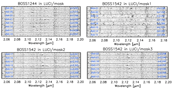
Figure 13: 2D spectra of HAEs in BOSS1244 and BOSS1542 observed via LBT/LUCI slit masks. Skyline residuals are visible as vertical lines with a higher noise level. The slit and spectrum ID in each mask are indicated. The upper left panel is the mask in the BOSS1244 field. The rest are the three masks in the BOSS1542 field.

Table A1 and Table A2 list the catalog of spectroscopically-confirmed HAEs and an [O III] emitter in BOSS1244 and BOSS1542.

Table A1: The sky positions, redshifts and total magnitudes at $K_{\rm s}$-band for the spectroscopically-confirmed HAEs in BOSS1244.

SlitMask	ID	R.A.	Decl.	Redshift	$K_{\rm s}$
		(J2000.0)	(J2000.0)	$z$	(mag)
	slit-2	12:43:24.01	$+$35:58:47.98	2.234	23.30$\pm$0.14
	slit-3	12:43:24.95	$+$35:58:38.59	2.235	22.79$\pm$0.08
	slit-4	12:43:27.98	$+$35:58:16.75	2.221	20.56$\pm$0.01
	slit-5	12:43:26.88	$+$35:58:06.74	2.235	22.45$\pm$0.08
	slit-13a	12:43:37.03	$+$35:56:29.58	2.229	20.39$\pm$0.01
	slit-14	12:43:36.69	$+$35:56:21.21	2.230	21.71$\pm$0.04
	slit-15	12:43:38.80	$+$35:56:11.17	2.226	21.80$\pm$0.05
	slit-17	12:43:29.71	$+$35:55:50.79	2.247	23.09$\pm$0.11
	slit-18	12:43:39.68	$+$35:55:40.21	2.227	22.08$\pm$0.04
MMIRS-mask1	slit-19	12:43:23.35	$+$35:55:31.22	2.235	20.56$\pm$0.01
	slit-20	12:43:38.43	$+$35:55:21.58	2.225	21.69$\pm$0.04
	slit-21	12:43:33.30	$+$35:55:10.79	2.220	22.52$\pm$0.07
	slit-22b	12:43:28.42	$+$35:54:59.30	2.213	21.54$\pm$0.04
	slit-23b	12:43:32.44	$+$35:54:46.00	2.250	21.77$\pm$0.03
	slit-26b	12:43:27.69	$+$35:53:57.44	2.253	22.08$\pm$0.06
	slit-27	12:43:29.22	$+$35:53:44.75	2.242	22.55$\pm$0.07
	slit-29	12:43:35.15	$+$35:53:16.44	2.255	21.74$\pm$0.04
	slit-30	12:43:29.54	$+$35:53:08.90	2.244	22.21$\pm$0.04
	slit-31	12:43:33.17	$+$35:52:50.99	2.245	22.18$\pm$0.05
	slit-1	12:44:13.61	$+$36:02:58.60	2.243	22.72$\pm$0.08
	slit-2	12:44:34.29	$+$36:06:55.98	2.244	22.42$\pm$0.09
	slit-3	12:44:33.60	$+$36:06:35.31	2.240	22.96$\pm$0.13
	slit-4	12:44:35.55	$+$36:04:20.98	2.239	22.41$\pm$0.07
	slit-5	12:44:33.48	$+$36:05:20.73	2.229	22.66$\pm$0.06
	slit-6	12:44:32.00	$+$36:05:04.60	2.253	21.95$\pm$0.05
	slit-7	12:44:30.59	$+$36:05:21.79	2.251	21.71$\pm$0.03
	slit-8	12:44:28.04	$+$36:03:52.50	2.245	21.54$\pm$0.03
MMIRS-mask2	slit-9	12:44:25.62	$+$36:03:59.77	2.247	21.87$\pm$0.04
	slit-10	12:44:23.73	$+$36:03:54.10	2.244	23.27$\pm$0.09
	slit-11	12:44:22.41	$+$36:03:24.96	2.253	22.58$\pm$0.09
	slit-12	12:44:17.83	$+$36:05:39.97	2.242	23.06$\pm$0.10
	slit-13	12:44:17.54	$+$36:05:15.89	2.248	22.67$\pm$0.10
	slit-16	12:44:15.86	$+$36:03:54.11	2.244	22.91$\pm$0.07
	slit-17	12:44:13.61	$+$36:02:58.60	2.250	22.44$\pm$0.08
	slit-20	12:44:08.17	$+$36:04:02.92	2.248	22.27$\pm$0.09
	slit-21	12:44:07.75	$+$36:03:13.92	2.248	21.14$\pm$0.04
	slit-22	12:44:05.18	$+$36:04:44.78	2.244	23.26$\pm$0.10
	slit-10	12:43:43.41	$+$35:54:49.69	2.231	22.06$\pm$0.06
	slit-11	12:43:42.66	$+$35:54:53.55	2.228	23.12$\pm$0.09
	slit-12	12:43:40.61	$+$35:54:08.32	2.217	20.50$\pm$0.02
LUCI-mask	slit-14	12:43:39.09	$+$35:54:03.71	2.246	20.54$\pm$0.01
	slit-21c	12:43:32.43	$+$35:54:46.07	2.249	21.77$\pm$0.03
	slit-23	12:43:29.86	$+$35:55:57.53	2.246	22.27$\pm$0.04
	slit-25c	12:43:28.44	$+$35:54:59.41	2.214	21.54$\pm$0.04
	slit-26c	12:43:27.68	$+$35:53:57.40	2.253	22.08$\pm$0.06

Note. — ^aslit-13 in MMIRS-mask1 is the QSO5 listed in Table 4. ^bslit-22, slit-23 and slit-26 in MMIRS-mask1 are the same with ^cslit-25, slit-21 and slit-26 in LUCI-mask. Their measured redshifts are consistent.

Table A2: The sky positions, redshifts and total magnitudes at $K_{\rm s}$-band for the spectroscopically-confirmed HAEs in BOSS1542.

SlitMask	ID	R.A.	Decl.	Redshift	$K_{\rm s}$
		(J2000.0)	(J2000.0)	$z$	(mag)
	slit-1	15:42:50.52	$+$38:58:18.48	2.244	22.59$\pm$0.10
	slit-4	15:42:36.90	$+$38:58:17.55	2.239	22.54$\pm$0.06
	slit-6a	15:42:34.96	$+$38:59:09.63	2.243	22.37$\pm$0.09
	slit-7	15:42:46.90	$+$38:59:49.53	2.229	22.33$\pm$0.07
	slit-8	15:42:41.55	$+$38:59:59.62	2.227	23.31$\pm$0.14
	slit-10	15:42:41.04	$+$39:00:19.09	2.251	22.09$\pm$0.05
	slit-11	15:42:36.31	$+$39:00:18.43	2.240	22.69$\pm$0.10
MMIRS-mask2	slit-15	15:42:42.66	$+$39:01:40.51	2.206	22.17$\pm$0.06
	slit-17	15:42:47.98	$+$39:02:22.66	2.211	22.05$\pm$0.06
	slit-21	15:42:48.39	$+$39:03:35.89	2.213	23.48$\pm$0.17
	slit-23	15:42:47.58	$+$39:03:49.58	2.215	22.82$\pm$0.11
	slit-24	15:42:39.88	$+$39:03:39.26	2.253	23.71 $\pm$0.22
	slit-25	15:42:40.60	$+$39:03:51.47	2.216	22.78$\pm$0.10
	slit-27b	15:42:29.55	$+$39:03:47.10	3.302	22.72$\pm$0.07
	slit-11	15:42:49.44	$+$38:51:58.53	2.256	22.10$\pm$0.06
	slit-14	15:42:52.83	$+$38:50:31.18	2.237	22.44$\pm$0.07
	slit-15	15:42:51.55	$+$38:50:29.29	2.241	21.63$\pm$0.06
LUCI-mask1	slit-16	15:42:57.86	$+$38:49:40.00	2.269	18.94 $\pm$0.02
	slit-17	15:42:56.87	$+$38:49:28.27	2.238	22.62$\pm$0.11
	slit-19	15:42:50.72	$+$38:49:41.08	2.241	22.27$\pm$0.08
	slit-20	15:42:52.78	$+$38:48:28.48	2.246	22.77$\pm$0.11
	slit-21	15:42:45.24	$+$38:48:30.69	2.238	22.06$\pm$0.05
	slit-10	15:42:45.35	$+$38:54:52.78	2.215	23.06$\pm$0.15
	slit-11	15:42:48.24	$+$38:54:18.03	2.238	22.12$\pm$0.08
	slit-12c	15:42:47.01	$+$38:53:42.34	2.241	19.42$\pm$0.01
LUCI-mask2	slit-13	15:42:49.56	$+$38:53:20.48	2.243	20.77$\pm$0.07
	slit-14	15:42:50.51	$+$38:52:14.80	2.242	22.78$\pm$0.07
	slit-15	15:42:49.44	$+$38:51:58.44	2.258	22.10$\pm$0.06
	slit-17	15:42:49.77	$+$38:52:50.46	2.241	22.94$\pm$0.11
	slit-12	15:42:32.86	$+$38:59:27.41	2.242	22.12$\pm$0.05
	slit-13d	15:42:34.97	$+$38:59:09.56	2.244	22.37$\pm$0.09
	slit-14	15:42:29.92	$+$38:58:33.08	2.242	22.88$\pm$0.12
LUCI-mask3	slit-17	15:42:42.12	$+$38:58:20.20	2.237	21.64$\pm$0.06
	slit-18	15:42:40.69	$+$38:58:03.00	2.242	20.24 $\pm$0.05
	slit-21	15:42:41.55	$+$38:56:50.88	2.240	21.75$\pm$0.05
	slit-22	15:42:43.27	$+$38:56:31.21	2.238	21.64$\pm$0.05

Note. — ^aslit-6 in MMIRS-mask2 is the same with ^dslit-13 in LUCI-mask3, and the measured redshift is consistent. ^bslit-27 in MMIRS-mask2 is an [O III] emitter. ^cslit-12 in LUCI-mask2 is the QSO3 listed in Table 4.

References

- An et al. (2014) An, F. X., Zheng, X. Z., Wang, W.-H., et al. 2014, ApJ, 784, 152, doi: 10.1088/0004-637X/784/2/152
- Arrigoni Battaia et al. (2015) Arrigoni Battaia, F., Hennawi, J. F., Prochaska, J. X., & Cantalupo, S. 2015, ApJ, 809, 163, doi: 10.1088/0004-637X/809/2/163
- Bagchi et al. (2017) Bagchi, J., Sankhyayan, S., Sarkar, P., et al. 2017, ApJ, 844, 25, doi: 10.3847/1538-4357/aa7949
- Bamford et al. (2009) Bamford, S. P., Nichol, R. C., Baldry, I. K., et al. 2009, MNRAS, 393, 1324, doi: 10.1111/j.1365-2966.2008.14252.x
- Beers et al. (1990) Beers, T. C., Flynn, K., & Gebhardt, K. 1990, AJ, 100, 32, doi: 10.1086/115487
- Belli et al. (2018) Belli, S., Contursi, A., & Davies, R. I. 2018, MNRAS, 478, 2097, doi: 10.1093/mnras/sty1236
- Bond et al. (1996) Bond, J. R., Kofman, L., & Pogosyan, D. 1996, Nature, 380, 603, doi: 10.1038/380603a0
- Borisova et al. (2016) Borisova, E., Cantalupo, S., Lilly, S. J., et al. 2016, ApJ, 831, 39, doi: 10.3847/0004-637X/831/1/39
- Bower et al. (1992) Bower, R. G., Lucey, J. R., & Ellis, R. S. 1992, MNRAS, 254, 601, doi: 10.1093/mnras/254.4.601
- Cai et al. (2016) Cai, Z., Fan, X., Peirani, S., et al. 2016, ApJ, 833, 135, doi: 10.3847/1538-4357/833/2/135
- Cai et al. (2017a) Cai, Z., Fan, X., Bian, F., et al. 2017a, ApJ, 839, 131, doi: 10.3847/1538-4357/aa6a1a
- Cai et al. (2017b) Cai, Z., Fan, X., Yang, Y., et al. 2017b, ApJ, 837, 71, doi: 10.3847/1538-4357/aa5d14
- Cai et al. (2018) Cai, Z., Hamden, E., Matuszewski, M., et al. 2018, ApJ, 861, L3, doi: 10.3847/2041-8213/aacce6
- Cai et al. (2019) Cai, Z., Cantalupo, S., Prochaska, J. X., et al. 2019, ApJS, 245, 23, doi: 10.3847/1538-4365/ab4796
- Cantalupo et al. (2014) Cantalupo, S., Arrigoni-Battaia, F., Prochaska, J. X., Hennawi, J. F., & Madau, P. 2014, Nature, 506, 63, doi: 10.1038/nature12898
- Casasola et al. (2018) Casasola, V., Magrini, L., Combes, F., et al. 2018, A&A, 618, A128, doi: 10.1051/0004-6361/201833052
- Casey et al. (2015) Casey, C. M., Cooray, A., Capak, P., et al. 2015, ApJ, 808, L33, doi: 10.1088/2041-8205/808/2/L33
- Cen & Ostriker (2000) Cen, R., & Ostriker, J. P. 2000, ApJ, 538, 83, doi: 10.1086/309090
- Chanchaiworawit et al. (2019) Chanchaiworawit, K., Guzmán, R., Salvador-Solé, E., et al. 2019, ApJ, 877, 51, doi: 10.3847/1538-4357/ab1a34
- Chiang et al. (2013) Chiang, Y.-K., Overzier, R., & Gebhardt, K. 2013, ApJ, 779, 127, doi: 10.1088/0004-637X/779/2/127
- Chiang et al. (2014) —. 2014, ApJ, 782, L3, doi: 10.1088/2041-8205/782/1/L3
- Chilingarian et al. (2015) Chilingarian, I., Beletsky, Y., Moran, S., et al. 2015, PASP, 127, 406, doi: 10.1086/680598
- Codis et al. (2012) Codis, S., Pichon, C., Devriendt, J., et al. 2012, MNRAS, 427, 3320, doi: 10.1111/j.1365-2966.2012.21636.x
- Collins et al. (2009) Collins, C. A., Stott, J. P., Hilton, M., et al. 2009, Nature, 458, 603, doi: 10.1038/nature07865
- Cooke et al. (2014) Cooke, E. A., Hatch, N. A., Muldrew, S. I., Rigby, E. E., & Kurk, J. D. 2014, MNRAS, 440, 3262, doi: 10.1093/mnras/stu522
- Cooke et al. (2016) Cooke, E. A., Hatch, N. A., Stern, D., et al. 2016, ApJ, 816, 83, doi: 10.3847/0004-637X/816/2/83
- Cucciati et al. (2014) Cucciati, O., Zamorani, G., Lemaux, B. C., et al. 2014, A&A, 570, A16, doi: 10.1051/0004-6361/201423811
- Cucciati et al. (2018) Cucciati, O., Lemaux, B. C., Zamorani, G., et al. 2018, A&A, 619, A49, doi: 10.1051/0004-6361/201833655
- Daddi et al. (2004) Daddi, E., Cimatti, A., Renzini, A., et al. 2004, ApJ, 617, 746, doi: 10.1086/425569
- Daddi et al. (2009) Daddi, E., Dannerbauer, H., Stern, D., et al. 2009, ApJ, 694, 1517, doi: 10.1088/0004-637X/694/2/1517
- Darvish et al. (2020) Darvish, B., Scoville, N. Z., Martin, C., et al. 2020, ApJ, 892, 8, doi: 10.3847/1538-4357/ab75c3
- Dekel & Birnboim (2006) Dekel, A., & Birnboim, Y. 2006, MNRAS, 368, 2, doi: 10.1111/j.1365-2966.2006.10145.x
- Dey et al. (2016) Dey, A., Lee, K.-S., Reddy, N., et al. 2016, ApJ, 823, 11, doi: 10.3847/0004-637X/823/1/11
- Dressler (1980) Dressler, A. 1980, ApJ, 236, 351, doi: 10.1086/157753
- Evrard et al. (2008) Evrard, A. E., Bialek, J., Busha, M., et al. 2008, ApJ, 672, 122, doi: 10.1086/521616
- Farina et al. (2011) Farina, E. P., Falomo, R., & Treves, A. 2011, MNRAS, 415, 3163, doi: 10.1111/j.1365-2966.2011.18931.x
- Franck & McGaugh (2016) Franck, J. R., & McGaugh, S. S. 2016, ApJ, 833, 15, doi: 10.3847/0004-637X/833/1/15
- Fukugita et al. (2004) Fukugita, M., Nakamura, O., Schneider, D. P., Doi, M., & Kashikawa, N. 2004, ApJ, 603, L65, doi: 10.1086/383222
- Geach et al. (2012) Geach, J. E., , D., Hickox, R. C., et al. 2012, MNRAS, 426, 679, doi: 10.1111/j.1365-2966.2012.21725.x
- Geach et al. (2008) Geach, J. E., Smail, I., Best, P. N., et al. 2008, MNRAS, 388, 1473, doi: 10.1111/j.1365-2966.2008.13481.x
- Gobat et al. (2015) Gobat, R., Daddi, E., Béthermin, M., et al. 2015, A&A, 581, A56, doi: 10.1051/0004-6361/201526274
- Goto et al. (2003) Goto, T., Yamauchi, C., Fujita, Y., et al. 2003, MNRAS, 346, 601, doi: 10.1046/j.1365-2966.2003.07114.x
- Green et al. (2011) Green, P. J., Myers, A. D., Barkhouse, W. A., et al. 2011, ApJ, 743, 81, doi: 10.1088/0004-637X/743/1/81
- Hatch et al. (2011) Hatch, N. A., De Breuck, C., Galametz, A., et al. 2011, MNRAS, 410, 1537, doi: 10.1111/j.1365-2966.2010.17538.x
- Hatch et al. (2014) Hatch, N. A., Wylezalek, D., Kurk, J. D., et al. 2014, MNRAS, 445, 280, doi: 10.1093/mnras/stu1725
- Hayashi et al. (2012) Hayashi, M., Kodama, T., Tadaki, K.-i., Koyama, Y., & Tanaka, I. 2012, ApJ, 757, 15, doi: 10.1088/0004-637X/757/1/15
- Hayashi et al. (2017) Hayashi, M., Kodama, T., Kohno, K., et al. 2017, ApJ, 841, L21, doi: 10.3847/2041-8213/aa71ad
- Hennawi et al. (2015) Hennawi, J. F., Prochaska, J. X., Cantalupo, S., & Arrigoni-Battaia, F. 2015, Science, 348, 779, doi: 10.1126/science.aaa5397
- Hill et al. (2020) Hill, R., Chapman, S., Scott, D., et al. 2020, MNRAS, doi: 10.1093/mnras/staa1275
- Hughes et al. (2013) Hughes, T. M., Cortese, L., Boselli, A., Gavazzi, G., & Davies, J. I. 2013, A&A, 550, A115, doi: 10.1051/0004-6361/201218822
- Husband et al. (2016) Husband, K., Bremer, M. N., Stott, J. P., & Murphy, D. N. A. 2016, MNRAS, 462, 421, doi: 10.1093/mnras/stw1520
- Ji et al. (2018) Ji, Z., Giavalisco, M., Williams, C. C., et al. 2018, ApJ, 862, 135, doi: 10.3847/1538-4357/aacc2c
- Jiang et al. (2018) Jiang, L., Wu, J., Bian, F., et al. 2018, Nature Astronomy, 2, 962, doi: 10.1038/s41550-018-0587-9
- Kartaltepe et al. (2019) Kartaltepe, J., Casey, C., Dickinson, M., et al. 2019, BAAS, 51, 395. https://arxiv.org/abs/1903.05026
- Kauffmann et al. (1999) Kauffmann, G., Colberg, J. M., Diaferio, A., & White, S. D. M. 1999, MNRAS, 303, 188, doi: 10.1046/j.1365-8711.1999.02202.x
- Kauffmann & White (1993) Kauffmann, G., & White, S. D. M. 1993, MNRAS, 261, 921, doi: 10.1093/mnras/261.4.921
- Kelson (2003) Kelson, D. D. 2003, PASP, 115, 688, doi: 10.1086/375502
- Kereš et al. (2009) Kereš, D., Katz, N., Fardal, M., Davé, R., & Weinberg, D. H. 2009, MNRAS, 395, 160, doi: 10.1111/j.1365-2966.2009.14541.x
- Kereš et al. (2005) Kereš, D., Katz, N., Weinberg, D. H., & Davé, R. 2005, MNRAS, 363, 2, doi: 10.1111/j.1365-2966.2005.09451.x
- Kikuta et al. (2019) Kikuta, S., Matsuda, Y., Cen, R., et al. 2019, PASJ, 71, L2, doi: 10.1093/pasj/psz055
- Kim et al. (2016) Kim, J.-W., Im, M., Lee, S.-K., et al. 2016, ApJ, 821, L10, doi: 10.3847/2041-8205/821/1/L10
- Koyama et al. (2021) Koyama, Y., Polletta, M. d. C., Tanaka, I., et al. 2021, MNRAS, 503, L1, doi: 10.1093/mnrasl/slab013
- Kraljic et al. (2018) Kraljic, K., Arnouts, S., Pichon, C., et al. 2018, MNRAS, 474, 547, doi: 10.1093/mnras/stx2638
- Kuchner et al. (2020) Kuchner, U., Aragón-Salamanca, A., Pearce, F. R., et al. 2020, MNRAS, doi: 10.1093/mnras/staa1083
- Kuiper et al. (2011) Kuiper, E., Hatch, N. A., Venemans, B. P., et al. 2011, MNRAS, 417, 1088, doi: 10.1111/j.1365-2966.2011.19324.x
- Kurk et al. (2004a) Kurk, J. D., Pentericci, L., Overzier, R. A., Röttgering, H. J. A., & Miley, G. K. 2004a, A&A, 428, 817, doi: 10.1051/0004-6361:20041819
- Kurk et al. (2004b) Kurk, J. D., Pentericci, L., Röttgering, H. J. A., & Miley, G. K. 2004b, A&A, 428, 793, doi: 10.1051/0004-6361:20040075
- Kurk et al. (2000) Kurk, J. D., Röttgering, H. J. A., Pentericci, L., et al. 2000, A&A, 358, L1. https://arxiv.org/abs/astro-ph/0005058
- Laigle et al. (2015) Laigle, C., Pichon, C., Codis, S., et al. 2015, MNRAS, 446, 2744, doi: 10.1093/mnras/stu2289
- Le Fèvre et al. (2015) Le Fèvre, O., Tasca, L. A. M., Cassata, P., et al. 2015, A&A, 576, A79, doi: 10.1051/0004-6361/201423829
- Lee et al. (2014a) Lee, K.-G., Hennawi, J. F., White, M., Croft, R. A. C., & Ozbek, M. 2014a, ApJ, 788, 49, doi: 10.1088/0004-637X/788/1/49
- Lee et al. (2016) Lee, K.-G., Hennawi, J. F., White, M., et al. 2016, ApJ, 817, 160, doi: 10.3847/0004-637X/817/2/160
- Lee et al. (2018) Lee, K.-G., Krolewski, A., White, M., et al. 2018, ApJS, 237, 31, doi: 10.3847/1538-4365/aace58
- Lee et al. (2014b) Lee, K.-S., Dey, A., Hong, S., et al. 2014b, ApJ, 796, 126, doi: 10.1088/0004-637X/796/2/126
- Lemaux et al. (2012) Lemaux, B. C., Gal, R. R., Lubin, L. M., et al. 2012, ApJ, 745, 106, doi: 10.1088/0004-637X/745/2/106
- Lemaux et al. (2014) Lemaux, B. C., Cucciati, O., Tasca, L. A. M., et al. 2014, A&A, 572, A41, doi: 10.1051/0004-6361/201423828
- Lemaux et al. (2018) Lemaux, B. C., Le Fèvre, O., Cucciati, O., et al. 2018, A&A, 615, A77, doi: 10.1051/0004-6361/201730870
- Liang et al. (2021) Liang, Y., Kashikawa, N., Cai, Z., et al. 2021, ApJ, 907, 3, doi: 10.3847/1538-4357/abcd93
- Libeskind et al. (2018) Libeskind, N. I., van de Weygaert, R., Cautun, M., et al. 2018, MNRAS, 473, 1195, doi: 10.1093/mnras/stx1976
- Lubin et al. (2000) Lubin, L. M., Brunner, R., Metzger, M. R., Postman, M., & Oke, J. B. 2000, ApJ, 531, L5, doi: 10.1086/312518
- Martin et al. (2014) Martin, D. C., Chang, D., Matuszewski, M., et al. 2014, ApJ, 786, 107, doi: 10.1088/0004-637X/786/2/107
- Martizzi et al. (2019) Martizzi, D., Vogelsberger, M., Artale, M. C., et al. 2019, MNRAS, 486, 3766, doi: 10.1093/mnras/stz1106
- McLeod et al. (2012) McLeod, B., Fabricant, D., Nystrom, G., et al. 2012, PASP, 124, 1318, doi: 10.1086/669044
- Miller et al. (2019) Miller, J. S. A., Bolton, J. S., & Hatch, N. 2019, MNRAS, 489, 5381, doi: 10.1093/mnras/stz2504
- Miller et al. (2018) Miller, T. B., Chapman, S. C., Aravena, M., et al. 2018, Nature, 556, 469, doi: 10.1038/s41586-018-0025-2
- Mo & White (1996) Mo, H. J., & White, S. D. M. 1996, MNRAS, 282, 347, doi: 10.1093/mnras/282.2.347
- Mukae et al. (2020) Mukae, S., Ouchi, M., Hill, G. J., et al. 2020, ApJ, 903, 24, doi: 10.3847/1538-4357/abb81b
- Muldrew et al. (2015) Muldrew, S. I., Hatch, N. A., & Cooke, E. A. 2015, MNRAS, 452, 2528, doi: 10.1093/mnras/stv1449
- Munari et al. (2013) Munari, E., Biviano, A., Borgani, S., Murante, G., & Fabjan, D. 2013, MNRAS, 430, 2638, doi: 10.1093/mnras/stt049
- Ocvirk et al. (2008) Ocvirk, P., Pichon, C., & Teyssier, R. 2008, MNRAS, 390, 1326, doi: 10.1111/j.1365-2966.2008.13763.x
- Onoue et al. (2018) Onoue, M., Kashikawa, N., Uchiyama, H., et al. 2018, PASJ, 70, S31, doi: 10.1093/pasj/psx092
- Oteo et al. (2018) Oteo, I., Ivison, R. J., Dunne, L., et al. 2018, ApJ, 856, 72, doi: 10.3847/1538-4357/aaa1f1
- Ouchi et al. (2005) Ouchi, M., Shimasaku, K., Akiyama, M., et al. 2005, ApJ, 620, L1, doi: 10.1086/428499
- Overzier (2016) Overzier, R. A. 2016, A&A Rev., 24, 14, doi: 10.1007/s00159-016-0100-3
- Pascarelle et al. (1996) Pascarelle, S. M., Windhorst, R. A., Keel, W. C., & Odewahn, S. C. 1996, Nature, 383, 45, doi: 10.1038/383045a0
- Peebles (1970) Peebles, P. J. E. 1970, AJ, 75, 13, doi: 10.1086/110933
- Peng et al. (2010) Peng, Y.-j., Lilly, S. J., Kovač, K., et al. 2010, ApJ, 721, 193, doi: 10.1088/0004-637X/721/1/193
- Pentericci et al. (2000) Pentericci, L., Kurk, J. D., Röttgering, H. J. A., et al. 2000, A&A, 361, L25. https://arxiv.org/abs/astro-ph/0008143
- Planck Collaboration et al. (2015) Planck Collaboration, Aghanim, N., Altieri, B., et al. 2015, A&A, 582, A30, doi: 10.1051/0004-6361/201424790
- Rosati et al. (1999) Rosati, P., Stanford, S. A., Eisenhardt, P. R., et al. 1999, AJ, 118, 76, doi: 10.1086/300934
- Sandrinelli et al. (2014) Sandrinelli, A., Falomo, R., Treves, A., Farina, E. P., & Uslenghi, M. 2014, MNRAS, 444, 1835, doi: 10.1093/mnras/stu1526
- Sandrinelli et al. (2018) Sandrinelli, A., Falomo, R., Treves, A., Scarpa, R., & Uslenghi, M. 2018, MNRAS, 474, 4925, doi: 10.1093/mnras/stx2822
- Santos et al. (2014) Santos, J. S., Altieri, B., Tanaka, M., et al. 2014, MNRAS, 438, 2565, doi: 10.1093/mnras/stt2376
- Santos et al. (2015) Santos, J. S., Altieri, B., Valtchanov, I., et al. 2015, MNRAS, 447, L65, doi: 10.1093/mnrasl/slu180
- Shandarin & Sunyaev (2009) Shandarin, S. F., & Sunyaev, R. A. 2009, A&A, 500, 19, doi: 10.1051/0004-6361/200912144
- Shandarin & Zeldovich (1989) Shandarin, S. F., & Zeldovich, Y. B. 1989, Reviews of Modern Physics, 61, 185, doi: 10.1103/RevModPhys.61.185
- Shi et al. (2020) Shi, K., Toshikawa, J., Cai, Z., Lee, K.-S., & Fang, T. 2020, ApJ, 899, 79, doi: 10.3847/1538-4357/aba626
- Shimakawa et al. (2014) Shimakawa, R., Kodama, T., Tadaki, K. I., et al. 2014, MNRAS, 441, L1, doi: 10.1093/mnrasl/slu029
- Shimakawa et al. (2018a) Shimakawa, R., Koyama, Y., Röttgering, H. J. A., et al. 2018a, MNRAS, 481, 5630, doi: 10.1093/mnras/sty2618
- Shimakawa et al. (2018b) Shimakawa, R., Kodama, T., Hayashi, M., et al. 2018b, MNRAS, 473, 1977, doi: 10.1093/mnras/stx2494
- Shimasaku et al. (2003) Shimasaku, K., Ouchi, M., Okamura, S., et al. 2003, ApJ, 586, L111, doi: 10.1086/374880
- Skibba et al. (2009) Skibba, R. A., Bamford, S. P., Nichol, R. C., et al. 2009, MNRAS, 399, 966, doi: 10.1111/j.1365-2966.2009.15334.x
- Sobral et al. (2012) Sobral, D., Best, P. N., Matsuda, Y., et al. 2012, MNRAS, 420, 1926, doi: 10.1111/j.1365-2966.2011.19977.x
- Sobral et al. (2013) Sobral, D., Smail, I., Best, P. N., et al. 2013, MNRAS, 428, 1128, doi: 10.1093/mnras/sts096
- Springel et al. (2005) Springel, V., White, S. D. M., Jenkins, A., et al. 2005, Nature, 435, 629, doi: 10.1038/nature03597
- Stark et al. (2015) Stark, C. W., White, M., Lee, K.-G., & Hennawi, J. F. 2015, MNRAS, 453, 311, doi: 10.1093/mnras/stv1620
- Steidel et al. (1998) Steidel, C. C., Adelberger, K. L., Dickinson, M., et al. 1998, ApJ, 492, 428, doi: 10.1086/305073
- Steidel et al. (2005) Steidel, C. C., Adelberger, K. L., Shapley, A. E., et al. 2005, ApJ, 626, 44, doi: 10.1086/429989
- Steidel et al. (2000) —. 2000, ApJ, 532, 170, doi: 10.1086/308568
- Steidel et al. (2003) —. 2003, ApJ, 592, 728, doi: 10.1086/375772
- Sunyaev & Zeldovich (1972) Sunyaev, R. A., & Zeldovich, Y. B. 1972, A&A, 20, 189
- Swinbank et al. (2007) Swinbank, A. M., Edge, A. C., Smail, I., et al. 2007, MNRAS, 379, 1343, doi: 10.1111/j.1365-2966.2007.12037.x
- Tadaki et al. (2011) Tadaki, K.-I., Kodama, T., Koyama, Y., et al. 2011, PASJ, 63, 437, doi: 10.1093/pasj/63.sp2.S437
- Tanaka et al. (2011) Tanaka, I., De Breuck, C., Kurk, J. D., et al. 2011, PASJ, 63, 415, doi: 10.1093/pasj/63.sp2.S415
- Tempel et al. (2014) Tempel, E., Stoica, R. S., Martínez, V. J., et al. 2014, MNRAS, 438, 3465, doi: 10.1093/mnras/stt2454
- Topping et al. (2016) Topping, M. W., Shapley, A. E., & Steidel, C. C. 2016, ApJ, 824, L11, doi: 10.3847/2041-8205/824/1/L11
- Topping et al. (2018) Topping, M. W., Shapley, A. E., Steidel, C. C., Naoz, S., & Primack, J. R. 2018, ApJ, 852, 134, doi: 10.3847/1538-4357/aa9f0f
- Toshikawa et al. (2020) Toshikawa, J., Malkan, M. A., Kashikawa, N., et al. 2020, ApJ, 888, 89, doi: 10.3847/1538-4357/ab5e85
- Toshikawa et al. (2012) Toshikawa, J., Kashikawa, N., Ota, K., et al. 2012, ApJ, 750, 137, doi: 10.1088/0004-637X/750/2/137
- Toshikawa et al. (2014) Toshikawa, J., Kashikawa, N., Overzier, R., et al. 2014, ApJ, 792, 15, doi: 10.1088/0004-637X/792/1/15
- Toshikawa et al. (2016) —. 2016, ApJ, 826, 114, doi: 10.3847/0004-637X/826/2/114
- Umehata et al. (2019) Umehata, H., Fumagalli, M., Smail, I., et al. 2019, Science, 366, 97, doi: 10.1126/science.aaw5949
- van Albada (1961) van Albada, G. B. 1961, AJ, 66, 590, doi: 10.1086/108469
- van de Voort et al. (2011) van de Voort, F., Schaye, J., Booth, C. M., Haas, M. R., & Dalla Vecchia, C. 2011, MNRAS, 414, 2458, doi: 10.1111/j.1365-2966.2011.18565.x
- van de Weygaert & Bond (2008) van de Weygaert, R., & Bond, J. R. 2008, Clusters and the Theory of the Cosmic Web, ed. M. Plionis, O. López-Cruz, & D. Hughes, Vol. 740, 335, doi: 10.1007/978-1-4020-6941-3_10
- Venemans et al. (2002) Venemans, B. P., Kurk, J. D., Miley, G. K., et al. 2002, ApJ, 569, L11, doi: 10.1086/340563
- Venemans et al. (2004) Venemans, B. P., Röttgering, H. J. A., Overzier, R. A., et al. 2004, A&A, 424, L17, doi: 10.1051/0004-6361:200400041
- Venemans et al. (2005) Venemans, B. P., Röttgering, H. J. A., Miley, G. K., et al. 2005, A&A, 431, 793, doi: 10.1051/0004-6361:20042038
- Venemans et al. (2007) —. 2007, A&A, 461, 823, doi: 10.1051/0004-6361:20053941
- Visvanathan & Sandage (1977) Visvanathan, N., & Sandage, A. 1977, ApJ, 216, 214, doi: 10.1086/155464
- Wang et al. (2016) Wang, T., Elbaz, D., Daddi, E., et al. 2016, ApJ, 828, 56, doi: 10.3847/0004-637X/828/1/56
- Whitaker et al. (2011) Whitaker, K. E., Labbé, I., van Dokkum, P. G., et al. 2011, ApJ, 735, 86, doi: 10.1088/0004-637X/735/2/86
- Williams et al. (2009) Williams, R. J., Quadri, R. F., Franx, M., van Dokkum, P., & Labbé, I. 2009, ApJ, 691, 1879, doi: 10.1088/0004-637X/691/2/1879
- Zheng et al. (2021) Zheng, X. Z., Cai, Z., An, F. X., Fan, X., & Shi, D. D. 2021, MNRAS, 500, 4354, doi: 10.1093/mnras/staa2882