How Fine-Tuning Allows for Effective Meta-Learning

Abstract

Representation learning has been widely studied in the context of meta-learning, enabling rapid learning of new tasks through shared representations. Recent works such as MAML have explored using fine-tuning-based metrics, which measure the ease by which fine-tuning can achieve good performance, as proxies for obtaining representations. We present a theoretical framework for analyzing representations derived from a MAML-like algorithm, assuming the available tasks use approximately the same underlying representation. We then provide risk bounds on the best predictor found by fine-tuning via gradient descent, demonstrating that the algorithm can provably leverage the shared structure. The upper bound applies to general function classes, which we demonstrate by instantiating the guarantees of our framework in the logistic regression and neural network settings. In contrast, we establish the existence of settings where any algorithm, using a representation trained with no consideration for task-specific fine-tuning, performs as well as a learner with no access to source tasks in the worst case. This separation result underscores the benefit of fine-tuning-based methods, such as MAML, over methods with “frozen representation” objectives in few-shot learning.

1 Introduction

Meta-learning (Thrun & Pratt, 2012) has emerged as an essential tool for quickly adapting prior knowledge to a new task with limited data and computational power. In this context, a meta-learner has access to some different but related source tasks from a shared environment. The learner aims to uncover some inductive bias from the source tasks to reduce sample and computational complexity for learning a new task from the same environment. One of the most promising methods is representation learning (Bengio et al., 2013), i.e., learning a feature extractor (or a common representation) from the source tasks. At test time, a learner quickly adapts to the new task by fine-tuning the representation and retraining the final layer(s) (see, e.g., prototype networks (Snell et al., 2017)). Substantial improvement over directly learning from a single task is expected in few-shot learning (Antoniou et al., 2018), a setting that naturally arises in many applications including reinforcement learning (Mendonca et al., 2019; Finn et al., 2017), computer vision (Nichol et al., 2018), federated learning (McMahan et al., 2017) and robotics (Al-Shedivat et al., 2017).

The empirical success of representation learning has led to an increased interest in theoretical analyses of underlying phenomena. Recent work assumes an explicitly shared representation across tasks (Du et al., 2020; Tripuraneni et al., 2020b, a; Saunshi et al., 2020; Balcan et al., 2015). For instance, Du et al. (2020) shows a generalization risk bound consisting of an irreducible representation error and estimation error. Without fine-tuning the whole network, the representation error accumulates to the target task and is irreducible even with infinite target labeled samples. Due to the lack of (representation) fine-tuning during training, we refer to these methods as making use of “frozen representation” objectives. This result is consistent with empirical findings, which suggest substantial performance gains associated with fine-tuning the whole network, compared to just learning the final linear layer (Chen et al., 2020; Salman et al., 2020).

Requiring tasks to be linearly separable on the same features is also unrealistic for transferring knowledge to other domains (e.g., from ImageNet to medical images (Raghu et al., 2019)). Therefore, we consider a more realistic setting, where the available tasks only approximately share the same representation. We propose a theoretical framework for analyzing the sample complexity of fine-tuning using a representation derived from a MAML-like algorithm. We show that fine-tuning quickly adapts to new tasks, requiring fewer samples in certain cases compared to methods using “frozen representation” objectives (as studied in Du et al. (2020), and will be formalized in Section 2.2). To the best of our knowledge, no prior studies exist beyond fine-tuning a linear model (Denevi et al., 2018; Konobeev et al., 2020; Collins et al., 2020a; Lee et al., 2020) or only the task-specific layers (Du et al., 2020; Tripuraneni et al., 2020b, a; Mu et al., 2020). In particular, our work can be viewed as a continuation of the work presented in Tripuraneni et al. (2020b), where the authors have acknowledged that the framework does not incorporate representation fine-tuning, and thus is a promising line of future work.

The following outlines this paper and its contributions:

• In Section 2, we outline the general setting and overall assumptions.

• In Section 3, we provide an in-depth analysis of the ($d$-dimensional) linear representation setting. First, we show that our MAML-like algorithm achieves a rate of $r_{source}=O(\frac{kd}{n_{\mathrm{S}}T}+\frac{k}{n_{\mathrm{S}}}+\delta_{0}\sqrt{\frac{\operatorname{tr}{\Sigma}}{n_{\mathrm{S}}}})$ on the source tasks and $O(\frac{k}{n_{\mathrm{T}}}+\delta_{0}\sqrt{\frac{\operatorname{tr}{\Sigma}}{n_{\mathrm{T}}}}+r_{source})$ on the target when the norm of the representation change is bounded by $\delta_{0}$, showing that fine-tuning can handle the approximately-shared representation setting. In contrast, “frozen representation” methods have a minimax rate of $\Omega(d/n_{\mathrm{T}})$ on the target task under certain task distributions, demonstrating that prior methods can fail.

• In Section 4, we extend the analysis to general function classes. Our result provides bounds of the form

  $$\varepsilon_{\mathrm{OPT}}+\varepsilon_{\mathrm{EST}}+\varepsilon_{\mathrm{REPR}},$$

  where $\varepsilon_{\mathrm{OPT}}$ is the optimization error, $\varepsilon_{\mathrm{EST}}$ is the estimation error, and $\varepsilon_{\mathrm{REPR}}$ stands for representation error.

  The optimization error naturally arises when the output of optimization procedure reaches an $\varepsilon_{\mathrm{OPT}}$-approximate minimum. To control $\varepsilon_{\mathrm{OPT}}$, our analysis accounts for nonconvexity introduced by representation fine-tuning, which is presented as a self-contained result in Section LABEL:sec:pgd-performance-bound.

  The estimation error $\varepsilon_{\mathrm{EST}}$ stems from fine-tuning the target parameters with finite $n_{\mathrm{T}}$ samples. It therefore scales with $1/\sqrt{n_{\mathrm{T}}}$ and is controlled by the (Rademacher) complexity of the target fine-tuning set.

  Finally, the representation error $\varepsilon_{\mathrm{REPR}}$ is the error associated with learning the centered representation while adapting to the task-specific deviations. Therefore it naturally consists of two terms: one term scales with $1/\sqrt{n_{\mathrm{S}}T}$ on learning the centered representation jointly with all $T$ source tasks; and the other term scales with $1/\sqrt{n_{\mathrm{S}}}$ on the small adaptation to each source task.

• In Section 5, we instantiate our guarantees in the logistic regression and two-layer neural network settings.

• In Section 6, we extend the separation result presented in Section 3 to a non-linear setting.

• In Section 7, we experimentally verify the separation result in the linear setting from Section 3.

1.1 Related Work

The empirical success of MAML (Finn et al., 2017) or, more generally, meta-learning, invokes further theoretical analysis from both statistical and optimization perspectives. A flurry of work engages in developing more efficient and theoretically-sound optimization algorithms (Antoniou et al., 2018; Nichol et al., 2018; Li et al., 2017) or showing convergence analysis (Fallah et al., 2020; Zhou et al., 2019; Rajeswaran et al., 2019; Collins et al., 2020b). Inspired by MAML, a line of gradient-based meta-learning algorithms have been widely used in practice Nichol et al. (2018); Al-Shedivat et al. (2017); Jerfel et al. (2018). Much follow-up work focused on online-setting with regret bounds (Denevi et al., 2018; Finn et al., 2019; Khodak et al., 2019; Balcan et al., 2015; Alquier et al., 2017; Bullins et al., 2019; Pentina & Lampert, 2014).

The statistical analysis of meta-learning can be traced back to Baxter (2000); Maurer & Jaakkola (2005), with a principle of inductive bias learning. Following the same setting, Amit & Meir (2018); Konobeev et al. (2020); Maurer et al. (2016); Pentina & Lampert (2014) assume a shared meta distribution for sampling the source tasks and measure generalization error/gap averaged over the meta distribution. Another line of work connects the target performance to source data with some distance measure between distributions (Ben-David & Borbely, 2008; Ben-David et al., 2010; Mohri & Medina, 2012). Finally, another series of works studied the benefits of using additional “side information” provided with a task for specializing the parameters of an inner algorithm (Denevi et al., 2020, 2021).

The hardness of meta-learning also attracts some investigation under various settings. Some recent work studies the meta-learning performance in worst-case setting (Collins et al., 2020b; Hanneke & Kpotufe, 2020a, b; Kpotufe & Martinet, 2018; Lucas et al., 2020). Hanneke & Kpotufe (2020a) provides a no-free-lunch result with problem-independent minimax lower bound, and Konobeev et al. (2020) also provide problem-dependent lower bound on a simple linear setting.

2 General Setting

2.1 Notation

Let $[n]\coloneqq\left\{1,\dots,n\right\}$. We denote the vector $L_{2}$-norm as $\left\lVert\cdot\right\rVert_{2}$, and the matrix Frobenius norm as $\left\lVert\cdot\right\rVert_{F}$. Additionally, $\left\langle\cdot,\cdot\right\rangle$ can denote either the Euclidean inner product or the Frobenius inner product between matrices.

For a matrix $A$, we let $\sigma_{i}(A)$ denote its $i^{\text{th}}$ largest singular value. Additionally, for positive semidefinite $A$, we write $\lambda_{\max}(A)$ and $\lambda_{\min}(A)$ for its largest and smallest eigenvalues, and $A^{1/2}$ for its principal square root. We write $P_{A}$ for the projection onto the column span of $A$, denoted $\operatorname{Col}{A}$, and $P_{A}^{\perp}\coloneqq I-P_{A}$ for the projection onto its complement.

We use standard $O,\Theta$, and $\Omega$ notation to denote orders of growth. We also use $a\lesssim b$ or $a\ll b$ to indicate that $a=O(b)$. Finally, we write $a\asymp b$ for $a=\Theta(b)$.

2.2 Problem Setting

We assume that the learner has access to $T$ source tasks. Every task $t\in[T]$ is associated with a distribution $\mu_{t}$ over the set $\mathcal{X}\times\mathcal{Y}$ of input-label pairs. We consider $\mathcal{X}\subseteq\mathbb{R}^{d}$ and $\mathcal{Y}\subseteq\mathbb{R}$ throughout. For every task, the learner observes $n_{\mathrm{S}}$ i.i.d. samples $\left\{(x_{i,t},y_{i,t})\right\}_{i\in[n_{\mathrm{S}}]}$ from $\mu_{t}$. We collect these inputs into matrices $X_{t}\in\mathbb{R}^{n_{\mathrm{S}}\times d}$ and labels into vectors $y_{t}\in\mathbb{R}^{n_{\mathrm{S}}}$ for convenience. Finally, we measure learner performance using the loss function $\ell:\mathbb{R}\times\mathcal{Y}\to\mathbb{R}$.

We aim to find a common structure across the source tasks that could be leveraged for learning future tasks. As done by Du et al. (2020), we study the case where the common structure is given by a representation, a mapping $\phi:\mathcal{X}\to\mathcal{Z}$ from the input space to a latent space $\mathcal{Z}\subseteq\mathbb{R}^{k}$. We assume that these representations lie in a function class $\mathcal{F}$ parameterized by some normed space. In contrast to prior work however, we do not assume the existence of a common representation – instead, each source task has an associated representation $\phi_{\theta_{t}}$ close to a fixed representation $\phi_{\theta_{0}}$, i.e. $\left\lVert\theta_{t}-\theta_{0}\right\rVert$ is small. As before, we apply a task-specific linear transformation to the representation to obtain the final prediction. Formally, the predictor for task $t\in[T]$ is given by $x\mapsto\left\langle w_{t},\phi_{t}(x)\right\rangle$. We then consider the following optimization problem for some $\delta_{0}>0$:

$$\min_{\theta_{0}}\min_{\begin{subarray}{c}\theta_{t},w_{t}\\ \left\lVert\theta_{t}-\theta_{0}\right\rVert\leq\delta_{0}\end{subarray}}\frac{1}{n_{\mathrm{S}}T}\sum_{t=1}^{T}\sum_{i=1}^{n_{\mathrm{S}}}\ell(\left\langle w_{t},\phi_{\theta_{t}}(x_{i,t})\right\rangle,y_{i,t}).$$ (1)

We will refer to the procedure above as AdaptRep, as it can be intuitively described as finding an initialization $\phi$ in representation space such that there exists a good representation nearby for every task (and thus a learner simply needs a small adaptation/fine-tuning step to achieve good performance). We note that the objective can be viewed as a constrained form of algorithms found in the literature such as iMAML (Rajeswaran et al., 2019) and Meta-MinibatchProx (Zhou et al., 2019). However, we do not have a train-validation split, as is widespread in practice. This setup is motivated by results in Bai et al. (2020), which show that data splitting may not be preferable performance-wise, assuming realizability. Furthermore, empirical evaluations have demonstrated successes despite the lack of such a split (Zhou et al., 2019).

Let $\theta_{0}$ be the initialization obtained from (1), which we will now use to learn future tasks. More concretely, let $\mu_{T+1}$ be a distribution over $\mathcal{X}\times\mathcal{Y}$ from which we have $n_{\mathrm{T}}$ i.i.d. samples $\left\{(x_{i},y_{i})\right\}_{i\in[n_{\mathrm{T}}]}$. As before, we collect these samples into a matrix $X\in\mathbb{R}^{n_{\mathrm{T}}\times d}$ and a vector $y\in\mathbb{R}^{n_{\mathrm{T}}}$. We then adapt to the target task by solving

$$\min_{\begin{subarray}{c}\theta,w\\ \left\lVert\theta-\theta_{0}\right\rVert\leq\delta_{0}\end{subarray}}\frac{1}{2n_{\mathrm{T}}}\sum_{i=1}^{n_{\mathrm{T}}}\ell(\left\langle w,\phi_{\theta}(x_{i})\right\rangle,y_{i}).$$ (2)

In the following sections, we will analyze the performance of the learned predictor for the population loss:

$$\mathcal{L}_{\mu_{T+1}}(\theta,w)\coloneqq\frac{1}{2}\mathbb{E}_{(x,y)\sim\mu_{T+1}}\left[\ell(\left\langle w,\phi_{\theta}(x)\right\rangle,y)\right].$$

We focus on the few-shot learning setting for the target task, where we assume limited access to target data, and a learner needs to effectively use the source tasks to learn the target task quickly.

For AdaptRep to be sensible, we need to ensure the existence of a desirable initialization. We do so by assuming that there exists an initialization $\theta_{0}^{\ast}$ such that for any $t\in[T]$, there exists a representation $\theta_{t}^{\ast}$ with $\left\lVert\theta_{t}^{\ast}-\theta_{0}^{\ast}\right\rVert\leq\delta_{0}$ and a predictor $w_{t}^{\ast}$ so that $\mu_{t}$ is given by

$$x\sim p_{t},\quad y\ |\ x\sim q(\cdot|\left\langle w_{t}^{\ast},\phi_{\theta_{t}}^{\ast}(x)\right\rangle)$$

with distribution $q$ to model some addictive noise. Specifically, in regression, we set $\mathbb{E}\left[y_{t}\ \middle|\ x\right]=\left\langle w_{t}^{\ast},\phi_{\theta_{t}}^{\ast}(x)\right\rangle$. With an appropriate choice of loss function $\ell$, we can guarantee that the optimal predictor under the population loss is $x\mapsto\left\langle w_{t}^{\ast},\phi_{t}^{\ast}(x)\right\rangle$.

Throughout the paper, we assume the existence of an oracle during source training time for solving (1), as in Du et al. (2020); Tripuraneni et al. (2020b). For detailed analyses of source training optimization, we refer the reader to Ji et al. (2020); Wang et al. (2020). Nevertheless, representation fine-tuning introduces nonconvexity during target time not present in prior work, where one only needed to solve the convex problem of optimizing a final linear layer. Thus, our bounds explicitly take into account optimization performance on (2). To this end, we analyze the use of projected gradient descent (PGD), which applies to a wide variety of settings, under certain loss landscape assumptions. These standalone results are also provided in Section LABEL:sec:pgd-performance-bound.

As a point of comparison with AdaptRep, we will also be analyzing the “frozen representation” objective used in Du et al. (2020); Tripuraneni et al. (2020b). In particular, using the notation introduced above, such objectives consider the following optimization problem:

$$\min_{\theta_{0}}\min_{w_{t}}\frac{1}{n_{\mathrm{S}}T}\sum_{t=1}^{T}\sum_{i=1}^{n_{\mathrm{S}}}\ell(\left\langle w_{t},\phi_{\theta_{0}}(x_{i,t})\right\rangle,y_{i,t}).$$ (3)

Due to the fact that the representation, once chosen, is fixed/frozen for all source tasks, we refer to the representation learning method above as FrozenRep throughout the rest of the paper. In Sections 3.4 and 6, we will demonstrate that unlike with AdaptRep, there exists cases where FrozenRep is unable to take advantage of the fact that the tasks approximately share representations.

3 AdaptRep in the Linear Setting

To illustrate the theory, we first examine AdaptRep in the linear setting. That is, we consider the set of linear transformations $\mathbb{R}^{d}\to\mathbb{R}^{k}$ for $d>k$, equipped with the Frobenius norm, so that $\phi_{B}(x)=B^{\top}x$. In this setting, we provide a performance bound for AdaptRep, and then exhibit a specific construction for which the baseline method in Du et al. (2020) fails to find useful representations.

3.1 Statistical Assumptions

We proceed to instantiate the data assumptions outlined in Section 2.2. First, we assume that the inputs for all tasks come from a common zero-mean distribution $p$, with covariance $\mathbb{E}_{x\sim p}\left[xx^{\top}\right]=\Sigma$. Let $\kappa=\lambda_{\max}(\Sigma)/\lambda_{\min}(\Sigma)$ be the condition number of this covariance matrix. As done by Du et al. (2020), we impose the following tail condition:

Assumption 3.1 (Sub-Gaussian input).

There exists $\rho>0$ such that if $x\sim p$, then $\Sigma^{-1/2}x$ is $\rho^{2}$-sub-Gaussian.

This assumption is used in the proofs to guarantee probabilistic tail bounds, and can be replaced with other conditions with appropriate modifications to the analysis. Finally, we define $q\left(\cdot\ \middle|\ \mu\right)\sim\mathcal{N}\left(\mu,\sigma^{2}\right)$ for a fixed $\sigma>0$.

We proceed to parametrize the tasks. Let $B^{\ast}$ be the ground truth initialization point, and $\Delta_{t}^{\ast}$ be the task-specific fine-tuning for task $t$, where $\left\lVert\Delta_{t}^{\ast}\right\rVert_{F}\leq\delta_{0}$. Furthermore, let $w_{t}^{\ast}\in\mathbb{R}^{k}$ be the task-specific predictor weights, which we combine into a matrix $W^{\ast}=[w_{1}^{\ast},\dots,w_{T}^{\ast}]\in\mathbb{R}^{k\times T}$.

Assumption 3.2 (Source task diversity).

For any $t\in[T]$, $\left\lVert w_{t}^{\ast}\right\rVert_{2}=\Theta(1)$, and $\sigma_{k}^{2}(W^{\ast})=\Omega(T/k)$.

Since the predictor weights all have $\Theta(1)$ norm, and thus $\sum_{i\in[k]}\sigma_{i}(W^{\ast})^{2}=\left\lVert W^{\ast}\right\rVert_{F}^{2}=\Theta(T)$, the assumption on $\sigma_{k}(W^{\ast})^{2}$ implies that the weights covers directions in $\mathbb{R}^{k}$ roughly evenly. This condition is satisfied with high probability when the $w^{\ast}_{t}$ are sampled from a sub-Gaussian distribution with well-conditioned covariance.

Finally, we evaluate the performance of the learner on a target task $\theta^{\ast}\coloneqq B^{\ast}w^{\ast}+\delta^{\ast}$ for some $w^{\ast}$ and $\left\lVert\delta^{\ast}\right\rVert_{2}\leq\delta_{0}$.

To gain an intuition for the parameters, note that $(B^{\ast}+\Delta_{t}^{\ast})w_{t}^{\ast}=B^{\ast}w_{t}^{\ast}+\delta_{t}^{\ast}$, where $\left\lVert\delta_{t}^{\ast}\right\rVert_{2}\lesssim\delta_{0}$ by the norm conditions in Assumption 3.2. Thus, we can think of the assumptions on the source predictor weights as ensuring their proximity to a rank-$k$ space.

Finally, as a convention since the parameterization is not unique, we define the optimal parameters so that $(B^{\ast})^{\top}\Sigma\delta_{t}^{\ast}=0$ for any $t\in[T]$. This results in no loss of generality, as we can always redefine $w_{t}^{\ast}$ and $\delta_{t}^{\ast}$ as such.

3.2 Training Procedure

(Source training) We can write the objective (1) in this setting as

$$\min_{B}\min_{\begin{subarray}{c}\Delta_{t},w_{t}\\ \left\lVert\Delta_{t}\right\rVert_{F}\leq\delta_{0}\end{subarray}}\frac{1}{2n_{\mathrm{S}}T}\sum_{t=1}^{T}\left\lVert y_{t}-X_{t}(B+\Delta_{t})w_{t}\right\rVert_{2}^{2}.$$

However, note that the objective does not impose any constraint on the predictor, as we can offload the norm of $\Delta_{t}$ onto $w_{t}$. Therefore, we instead consider the regularized source training objective

$$\min_{B}\min_{\Delta_{t},w_{t}}\frac{1}{2n_{\mathrm{S}}T}\sum_{t=1}^{T}\left\lVert y_{t}-X_{t}(B+\Delta_{t})w_{t}\right\rVert_{2}^{2}+\frac{\lambda}{2}\left\lVert\Delta_{t}\right\rVert_{F}^{2}+\frac{\gamma}{2}\left\lVert w_{t}\right\rVert_{2}^{2}.$$ (4)

As will be shown in Section A, the regularization is equivalent to regularizing $\sqrt{\lambda\gamma}\left\lVert\Delta_{t}w_{t}\right\rVert_{2}$, which is consistent with the intuition that $\delta_{t}^{\ast}$ has small norm.

(Target training) Letting $B_{0}$ be the obtained representation after orthonormalization, we adapt to the target task by optimizing

$$\mathcal{L}_{\beta}(\Delta,w)=\frac{1}{2n}\left\lVert y-\beta X\left(A_{B_{0}}+\Delta\right)(w_{0}+w)\right\rVert_{2}^{2},$$ (5)

where $A_{B_{0}}\coloneqq[B_{0}\ B_{0}]\in\mathbb{R}^{d\times 2k}$ and $w_{0}=[u,-u]$ for some unit-norm vector $u\in\mathbb{R}^{k}$. To optimize the objective, we perform PGD on (5) with

$$\mathcal{C}_{\beta}\coloneqq\left\{(\Delta,w)\ \middle|\ \left\lVert\Delta\right\rVert_{F}\leq c_{1}/\beta,\left\lVert w\right\rVert_{2}\leq c_{2}/\beta\right\}$$

as the feasible set, where we explicitly define $c_{1}$ and $c_{2}$ in Section A.

To understand the choice of training objective above, observe that the predictor can be written as

$$x\mapsto\beta(x^{\top}A_{B_{0}}w+x^{\top}\Delta w_{0}+x^{\top}\Delta w),$$

where the “antisymmetric” initialization scheme ensures that $A_{B_{0}}w_{0}=0$. Due to the choice of $\mathcal{C}_{\beta}$, the first two terms are of norm $O(1)$, while the last term is of norm $O(1/\beta)$. Therefore, for large enough $\beta$, we can treat the cross term $\Delta w$ as a negligible perturbation, and the predictor is approximately linear in the parameters. Indeed, one can show that $\mathcal{L}_{\beta}$ is thus approximately convex, guaranteeing that the best solution found by PGD is nearly optimal.

3.3 Performance Bound

Now, we provide a performance bound on the performance of the algorithm proposed in the previous section, which we prove in Section A. We define the following rates of interest:

$$r_{\mathrm{S}}(n_{\mathrm{S}},T) \coloneqq\frac{\sigma^{2}kd}{n_{\mathrm{S}}T}+\sigma\delta_{0}\left\lVert\Sigma\right\rVert_{2}^{1/2}\sqrt{\frac{kd}{n_{\mathrm{S}}T}}+\frac{\sigma^{2}k}{n_{\mathrm{S}}}+\frac{\sigma\delta_{0}}{\sqrt{n_{\mathrm{S}}}}\sqrt{\operatorname{tr}{\Sigma}}$$

$$r_{\mathrm{T}}^{(1)}(n_{\mathrm{T}}) \coloneqq kr_{\mathrm{S}}(n_{\mathrm{S}},T)+\frac{\sigma^{2}k}{n_{\mathrm{T}}}+\frac{\sigma\delta_{0}}{\sqrt{n_{\mathrm{T}}}}\sqrt{\operatorname{tr}\Sigma}$$

$$r_{\mathrm{T}}^{(2)}(n_{\mathrm{T}}) \coloneqq\frac{\sigma^{2}k}{n_{\mathrm{T}}}+\left[1+\sqrt{\frac{\kappa}{\lambda_{\min}}kr_{\mathrm{S}}(n_{\mathrm{S}},T)}\right]\frac{\sigma\delta_{0}}{\sqrt{n_{\mathrm{T}}}}\sqrt{\operatorname{tr}\Sigma}$$

Theorem 3.1 (Performance guarantee, linear representations).

Fix a failure probability $\delta\in(0,1)$. Assume that Assumptions 3.1 and 3.2 hold, and that $n_{\mathrm{S}}\gg\rho^{4}(d+\log(T/\delta))$ and $n_{\mathrm{T}}\gg\rho^{4}(d+\log(1/\delta))$. Then there are $(\lambda,\gamma,\beta,T_{\mathrm{PGD}},\eta,c_{1},c_{2})$ (specified in Section A) such that with probability at least $1-\delta$ over the random draw of all samples, the training procedure in Section 3.2 can find a parameter $\theta$ such that the excess risk on the target task is bounded by

$$\mathbb{E}\left[(x^{\top}\theta^{\ast}-x^{\top}\theta)^{2}\right]\lesssim\min\left(r_{\mathrm{T}}^{(1)}(n_{\mathrm{T}}),r_{\mathrm{T}}^{(2)}(n_{\mathrm{T}}),\frac{\sigma^{2}d}{n_{\mathrm{T}}}\right).$$

We briefly remark on the three available rates, which corresponds to three different subalgorithms depending on the amount of target data. Firstly, as will be proven in Section A, $r_{\mathrm{S}}$ is a performance bound on the learner during source training. Then:

1. In the most data-starved regime, we restrict the learner so that it can only adapt to learn $\delta^{\ast}$ for the target task to obtain the first rate. Notably, $r_{\mathrm{T}}^{(1)}$ incorporates the resulting irreducible source error in the form of $kr_{\mathrm{S}}(n_{\mathrm{S}},T)$.

2. The second rate $r_{\mathrm{T}}^{(2)}$ results when we allow the learner to adapt more (requiring more target samples) to reduce the irreducible error due to finite $n_{S}$. Observe that this additional complexity in the fine-tuning step is captured by the multiplicative factor that shrinks to $1$ in the limit of infinite source samples.

3. Finally, we can obtain the trivial $\sigma^{2}d/n_{\mathrm{T}}$ rate by ignoring $B_{0}$, which matches the minimax lower bound for standard linear regression (see e.g., Duchi (2016)).

3.4 A Hard Case for FrozenRep

In what follows, we demonstrate the existence of a family of task distributions satisfying the assumptions outlined in Section 3.1 that is difficult for the method in Du et al. (2020), which we will refer to as FrozenRep. More explicitly, we prove an $\Omega(d/n)$ minimax rate on the target task when using an FrozenRep-derived representation, even with access to infinite source tasks and data. Since this rate is achievable via training on the target task directly, this demonstrates that FrozenRep fails to capture the shared information between the tasks. In contrast, by specializing Theorem 3.1 to the proposed family of tasks, we will show that AdaptRep can indeed achieve a strictly faster statistical rate.

We proceed to explicitly define the objects in Section 3.1. Let $p$ be a Gaussian distribution on $\mathbb{R}^{d}$ with covariance

$$\Sigma=\begin{bmatrix}\varepsilon I_{d-k}&0\\ 0&I_{k}\\ \end{bmatrix}$$

for a fixed $\varepsilon\in(0,1)$. We define $E^{\ast},E_{k}\subset\mathbb{R}^{d}$ to be the eigenspaces corresponding to the first and second block of $\Sigma$, respectively, i.e.

$$E^{\ast}=\operatorname{Col}{\begin{bmatrix}\varepsilon I_{d-k}\\ 0\\ \end{bmatrix}}\quad\text{and}\quad E_{k}=\operatorname{Col}{\begin{bmatrix}0\\ I_{k}\\ \end{bmatrix}}.$$

Then, for an orthogonal matrix $B\in\mathbb{R}^{d\times k}$, define a corresponding task distribution given by

$$\theta=\frac{1}{\sqrt{2\varepsilon}}Bw+\delta,$$ (6)

where $w$ and $\delta$ are sampled uniformly at random from the unit spheres in $\mathbb{R}^{k}$ and $E_{k}$, respectively. The family of interest is the set of task distributions induced by any $B^{\ast}$ such that $\operatorname{Col}{B^{\ast}}\subset E^{\ast}$.

In this setting, we can write the FrozenRep objective in (3) as

$$\hat{B}=\operatorname*{argmin}_{B}\min_{w_{t}}\frac{1}{2n_{\mathrm{S}}T}\sum_{t\in[T]}\left\lVert y_{t}-X_{t}Bw_{t}\right\rVert_{2}^{2}.$$ (7)

First, we characterize the span of $\hat{B}$ in the limit of infinite source tasks and data. Intuitively, since both $B^{\ast}w$ and $\delta$ both lie in (distinct) rank-$k$ spaces, but $(1/\sqrt{2\varepsilon})\left\lVert\Sigma^{1/2}B^{\ast}w\right\rVert_{2}\leq\left\lVert\Sigma^{1/2}\delta\right\rVert_{2}$ for any $(w,\delta)$ from the task distribution (and thus the error along $\delta$ is larger), FrozenRep learns $E_{k}$ rather than $B^{\ast}$.

Lemma 3.1 (FrozenRep learns incorrect space).

Fix an orthogonal matrix $B^{\ast}\in\mathbb{R}^{d\times k}$ with $\operatorname{Col}{B^{\ast}}\subseteq E^{\ast}$, and assume that we sample task weights from the distribution in (6). Then, with infinitely many tasks and per-task samples $(n_{\mathrm{S}},T\to\infty)$, $\operatorname{Col}{\hat{B}}=E_{k}$.

The claim is proven in Section LABEL:sec:erm-hard-case-proofs. Although “incorrect”, it is unclear a priori that this choice of $\hat{B}$ is undesirable performance-wise – we now show that this indeed the case. In fact, any algorithm making use of $\hat{B}$, in the worst case, cannot perform any better than a learner that is constrained to only use target data.

Theorem 3.2 (FrozenRep minimax bound).

For an orthogonal matrix $B^{\ast}\in\mathbb{R}^{d\times k}$ whose column space lies in $E^{\ast}$, let $S_{B^{\ast}}$ be the set

$$S_{B^{\ast}}\coloneqq\left\{\frac{1}{\sqrt{2\varepsilon}}B^{\ast}w+\delta\ \middle|\ \left\lVert w\right\rVert_{2}\leq 1,\left\lVert\delta\right\rVert_{2}\leq 1,\delta\in E_{k}\right\}.$$

Then, with high probability over the draw of $n_{T}\gg d$ samples during target training, we have that

$$\min_{\begin{subarray}{c}\bar{B},\hat{w},\hat{\delta}\\ \operatorname{Col}{\bar{B}}=\operatorname{Col}{\hat{B}}\end{subarray}}\max_{\begin{subarray}{c}B^{\ast}\\ \theta^{\ast}\in S_{B^{\ast}}\end{subarray}}\mathbb{E}\left[\frac{1}{n_{T}}\left\lVert X(\theta^{\ast}-\bar{B}\hat{w}-\hat{\delta})\right\rVert_{2}^{2}\right]\gtrsim\frac{\sigma^{2}d}{n_{T}},$$

where $\hat{B}$ is the output of FrozenRep in the setting of Lemma 3.1, with the task distribution determined by $B^{\ast}$. The expectation is over the randomness in the labels $y\sim\mathcal{N}\left(X\theta^{\ast},\sigma^{2}I_{n_{\mathrm{T}}}\right)$. Furthermore, $\bar{B}$, $\hat{w}$, and $\hat{\delta}$ are measurable functions of $(X,y)$ to $\mathbb{R}^{d\times k},\mathbb{R}^{k},$ and $\mathbb{R}^{d}$, respectively.

The previous result, which we prove in Section LABEL:sec:erm-hard-case-proofs, shows that any procedure making use of target samples to learn a predictor of the form $\hat{B}\hat{w}+\hat{\delta}$ has a minimax rate of $\Omega(d/n)$. This includes target-time fine-tuning procedures used by methods in practice such as iMAML, MetaOptNet (Lee et al., 2019), and R2D2 (Bertinetto et al., 2019). Notably, this rate is achievable by performing linear regression solely on the target samples, reflecting that the FrozenRep learner failed to capture the shared task structure. In contrast, by specializing the guarantee of Theorem 3.1 to this setting, we have the following result:

Corollary 3.1.

Fix $k=\Theta(1)$ and $d\gg k$, and set $\varepsilon=k/d$. Furthermore, assume that $n_{\mathrm{S}}T\gtrsim d^{2}$, and $n_{\mathrm{S}}\geq n_{\mathrm{T}}\asymp d$. Then, for a fixed target task in $S_{B^{\ast}}$ as defined in Theorem 3.2, with probability at least $1-\delta$ over the draw of samples, the procedure outlined in Section 3.2 achieves excess risk bounded as

$$\mathbb{E}\left[(x^{\top}\theta^{\ast}-x^{\top}\hat{\theta})^{2}\right]\lesssim\min\left(\frac{\sigma}{\sqrt{n_{\mathrm{T}}}},\frac{\sigma^{2}d}{n_{\mathrm{T}}}\right).$$

In constrast to the rate above, the minimax rate in Theorem 3.2 remains bounded away from $0$ when $n_{\mathrm{T}}\asymp d$. Therefore, in addition to performing at least as well as the minimax rate for FrozenRep for any $n_{\mathrm{T}}\gtrsim d$, there exists a strict separation between the methods that widens as $n_{\mathrm{T}}\to\infty$. Furthermore, the guarantee can be achieved with finite source samples. Thus, we have established a setting where incorporating a notion of representation fine-tuning into meta-training is provably necessary for the meta-learner to succeed.

4 AdaptRep in the Nonlinear Setting

We now describe a general framework for analyzing fine-tuning in general function classes. To simplify the notation, we modify the setting described in Section 2.2 so that both the representation $\phi$ and task-specific weight vector $w$ are captured by one parameter $\theta\in\Theta$, with corresponding predictor $g_{\theta}$.

Throughout this section, we denote the population loss induced by a predictor $g$ as

$$\mathcal{L}^{g}_{\infty}(h):=\mathbb{E}_{(x,y)\sim\mu_{g}}\left[\ell(h(x),y)\right],$$

where $\mu_{g}$ samples $x\sim p$ and $y\ |\ x\sim q(\cdot|g(x))$. Additionally, we let $\mathcal{L}^{g}(h)$ denote the corresponding finite-sample quantity.

Furthermore, for a fixed parameter $\theta$ and a set $\mathcal{C}$, we define the set $\mathcal{A}^{\mathcal{C}}_{\theta}$ to be

$$\mathcal{A}_{\theta}^{\mathcal{C}}\coloneqq\left\{g_{\theta^{\prime}}\ \middle|\ \theta^{\prime}-\theta\in\mathcal{C}\right\}.$$

Intuitively, we can think of $\mathcal{C}$ as the possible ways a learner could adapt, and $\mathcal{A}^{\mathcal{C}}_{\theta}$ is the resulting set of possible predictors given an initialization $\theta$. For convenience, we define $\left(\mathcal{A}_{\theta}^{\mathcal{C}}\right)^{\otimes T}$ to be the set of functions mapping $\mathcal{X}^{T}\to\mathcal{Y}^{T}$ defined as

$$\left(\mathcal{A}_{\theta}^{\mathcal{C}}\right)^{\otimes T}\coloneqq\left\{(x_{i})_{i\in[T]}\mapsto(f_{i}(x_{i}))_{i\in[T]}\ \middle|\ f_{1},\dots,f_{T}\in\mathcal{A}_{\theta}^{\mathcal{C}}\right\}.$$

That is, $\left(\mathcal{A}_{\theta}^{\mathcal{C}}\right)^{\otimes T}$ can be interpreted as the set of possible choices of $T$ predictors for $T$ source tasks that are all close to some initialization $\theta$.

4.1 Training Procedure

The training procedure is defined by a set of possible initializations $\Theta_{0}\subseteq\Theta$, and fine-tuning sets $\mathcal{C}_{\mathrm{S}},\mathcal{C}_{\mathrm{T}}\subseteq\Theta$. We then rewrite the objective defined in (1) in terms of $\theta$ as

$$\theta_{0}=\operatorname*{argmin}_{\theta\in\Theta_{0}}\min_{g_{t}\in\mathcal{A}_{\theta}^{\mathcal{C}_{\mathrm{S}}}}\frac{1}{2n_{\mathrm{S}}T}\sum_{t=1}^{T}\sum_{i=1}^{n_{S}}\ell(g_{t}(x_{i,t}),y_{i,t}).$$ (8)

Note that $\mathcal{C}_{\mathrm{S}}$ is the feasible set of task-specific fine-tuning options for source training. Then, given samples from a target task $g^{\ast}$, we perform $T_{\mathrm{PGD}}$ steps of PGD with step size $\eta$ on the objective $\delta\mapsto\mathcal{L}^{g^{\ast}}(g_{\theta_{0}+\delta})$, with feasible fine-tuning set $\mathcal{C}_{\mathrm{T}}$.

4.2 Assumptions

We now outline the assumptions we make in this setting.

Assumption 4.1.

For any $y\in\mathcal{Y}$, $\ell(\cdot,y)$ is $1$-Lipschitz and convex, and that $\left|\ell(0,y)\right|\leq B$.

To ensure transfer from source to target, we impose the following condition, a specific instance of which was proposed by Du et al. (2020) in the linear setting, and proposed by Tripuraneni et al. (2020b) for general settings:

Assumption 4.2 (Source tasks are $(\nu,\varepsilon)$-diverse).

There exists constants $(\nu,\varepsilon)$ such that if $\rho$ is the distribution of target tasks, then for any $\theta\in\Theta_{0}$,

$$\mathbb{E}_{g^{\ast}\sim\rho}\left[\inf_{g\in\mathcal{A}_{\theta}^{\mathcal{C}_{\mathrm{T}}}}\mathcal{L}_{\infty}^{g^{\ast}}(g)-\mathcal{L}_{\infty}^{g^{\ast}}(g^{\ast})\right]\leq\frac{1}{\nu}\left[\frac{1}{T}\sum_{t=1}^{T}\inf_{g\in\mathcal{A}_{\theta}^{\mathcal{C}_{\mathrm{S}}}}\mathcal{L}_{\infty}^{g_{t}^{\ast}}(g)-\mathcal{L}_{\infty}^{g_{t}^{\ast}}(g_{t}^{\ast})\right]+\varepsilon.$$

That is, the average best-case performance on the set of target tasks is controlled by the task-averaged best-case performance on the source tasks.

The $(\nu,\varepsilon)$-diversity assumption ensures that optimizing $\theta$ for the average source task performance results in controlled average target task performance. Note that we weakened the condition in Tripuraneni et al. (2020b) to bound the average rather than worst-case target performance, as is more suitable for higher-dimensional settings.

Finally, we make several assumptions to ensure that PGD finds a solution close in performance to the optimal fine-tuning parameter in $\mathcal{C}_{\mathrm{T}}$. We remark that these assumptions are specific to the choice of fine-tuning algorithm.

Assumption 4.3 (Approximate linearity in fine-tuning).

Let $x_{1},\dots,x_{n_{\mathrm{T}}}$ be the set of target inputs. Then, there exists $\beta,L$ such that

$$\sup_{\delta\in\mathcal{C}_{T}}\frac{1}{n_{\mathrm{T}}}\sum_{i=1}^{n_{\mathrm{T}}}\left\lVert\nabla_{\theta}^{2}g_{\theta+\delta}(x_{i})\right\rVert_{2}^{2} \leq\beta^{2}\quad\text{and}\quad\sup_{\theta\in\Theta_{0}}\frac{1}{n_{\mathrm{T}}}\sum_{i=1}^{n_{\mathrm{T}}}\left\lVert\nabla_{\theta}g_{\theta}(x)\right\rVert_{2}^{2}\leq L^{2}.$$

Assumption 4.4.

$\sup_{\delta\in\mathcal{C}_{\mathrm{T}}}\left\lVert\delta\right\rVert_{2}\leq R$ for some $R$.

4.3 Performance Bound

Before we present the performance bound, recall that for a set $\mathcal{H}$ of functions $\mathbb{R}^{d}\to\mathbb{R}^{k}$ on $n$ samples, its Rademacher complexity $\mathcal{R}_{n}(\mathcal{H})$ on $n$ samples is given by

$$\mathcal{R}_{n}(\mathcal{H})\coloneqq\mathbb{E}_{\varepsilon,X}\left[\frac{1}{n}\left|\sup_{h\in\mathcal{H}}\sum_{i=1}^{n}\sum_{j=1}^{k}\varepsilon_{ij}h_{j}(x_{i})\right|\right],$$

where $(\varepsilon_{ij})$ are i.i.d. Rademacher random variables and $(x_{i})$ are i.i.d. samples from some (preset) distribution.

Theorem 4.1 (General Performance Bound).

Assume that Assumptions 4.1, 4.2, 4.3 and 4.4 all hold. Consider a learner following the training procedure outlined in Section 4.1, and let $(\theta_{t})$ be the set of iterates generated by PGD with appropriately chosen step size $\eta$ (specified in Section LABEL:sec:gen-perf-proofs). Then, with probability at least $1-\delta$ over the random draw of samples,

$$\mathbb{E}_{g^{\ast}\sim\rho}\left[\min_{t}\mathcal{L}^{g^{\ast}}_{\infty}(\theta_{t})-\mathcal{L}_{\infty}^{g^{\ast}}(\theta^{\ast}+\delta^{\ast})\right] \lesssim\underbrace{\beta R^{2}+R\sqrt{\frac{L^{2}+\beta^{2}R^{2}}{T_{\mathrm{PGD}}}}}_{\varepsilon_{\mathrm{OPT}}}+\underbrace{\frac{1}{\delta}\mathcal{R}_{n_{\mathrm{T}}}\left(\mathcal{A}_{\theta_{0}}^{\mathcal{C}_{\mathrm{T}}}\right)+\frac{B}{\delta\sqrt{n_{\mathrm{T}}}}}_{\varepsilon_{\mathrm{EST}}}$$

$$\qquad+\underbrace{\frac{1}{\nu}\left\{\frac{1}{\delta T}\mathcal{R}_{n_{\mathrm{S}}}\left[\bigcup_{\theta\in\Theta_{0}}\left(\mathcal{A}_{\theta}^{\mathcal{C}_{\mathrm{S}}}\right)^{\otimes T}\right]+\frac{B}{\delta\sqrt{n_{\mathrm{S}}T}}\right\}+\varepsilon}_{\varepsilon_{\mathrm{REPR}}}.$$

Note that the $\mathcal{R}_{n_{\mathrm{T}}}$ complexity term samples from $p$, while the $\mathcal{R}_{n_{\mathrm{S}}}$ complexity term samples from $p^{\otimes T}$, i.e. each draw is $T$ i.i.d. draws from $p$, concatenated.

Note that the Rademacher complexity terms above decays in most settings as

$$\mathcal{R}_{n_{\mathrm{T}}}(\mathcal{A}_{\theta_{0}}^{\mathcal{C}_{\mathrm{T}}}) \asymp O\left(\frac{\operatorname{diam}{\mathcal{C}_{\mathrm{T}}}}{\sqrt{n_{\mathrm{T}}}}\right)$$

$$\frac{1}{T}\mathcal{R}_{n_{\mathrm{S}}}\left[\bigcup_{\theta\in\Theta_{0}}\left(\mathcal{A}_{\theta}^{\mathcal{C}_{\mathrm{S}}}\right)^{\otimes T}\right] \asymp O\left(\frac{C(\Theta_{0})}{\sqrt{n_{\mathrm{S}}\mathrm{T}}}+\frac{\operatorname{diam}{\mathcal{C}_{\mathrm{S}}}}{\sqrt{n_{\mathrm{S}}}}\right),$$

where $C(\Theta_{0})$ represents some complexity measure of $\Theta_{0}$, and $\operatorname{diam}{\mathcal{C}_{\mathrm{S}}}$ and $\operatorname{diam}{\mathcal{C}_{\mathrm{T}}}$ represents a measure of the size of the fine-tuning sets $\mathcal{C}_{\mathrm{S}}$ and $\mathcal{C}_{\mathrm{T}}$. A full proof is provided in Section LABEL:sec:gen-perf-proofs. Nevertheless, we provide a brief intuition on the result, as well as how the assumptions contribute to the final bound. Let $\theta_{\mathrm{opt}}$ denote the best-performing solution found by PGD, $\theta_{\mathrm{ERM}}$ and $\bar{\theta}$ the ERM and population-level optimal solution in $\mathcal{A}_{\theta_{0}}^{\mathcal{C}_{\mathrm{T}}}$ respectively, and $\theta^{\ast}$ the ground truth predictor.

Optimization error ($\varepsilon_{\mathrm{OPT}}$). The difference in performance between $\theta_{\mathrm{opt}}$ and $\theta_{\mathrm{ERM}}$, i.e. the error due to the optimization procedure, is bounded by approximate linearity.

Estimation error ($\varepsilon_{\mathrm{EST}}$). By uniform convergence, $\theta_{\mathrm{ERM}}$ (and thus $\theta_{\mathrm{opt}}$) performs similarly to $\bar{\theta}$.

Representation/approximation error ($\varepsilon_{\mathrm{REPR}}$). Via the $(\nu,\varepsilon)$-diversity condition, $\bar{\theta}$ is connected to $\theta^{\ast}$ explicitly (that is, the performance on the target task is controlled by the performance on the source tasks). Furthermore, the performance over source tasks can be bounded via uniform convergence.

5 Case Studies

5.1 Multitask Logistic Regression

To illustrate our framework, we analyze the performance of AdaptRep on logistic regression, as done by Tripuraneni et al. (2020b). In this setting, we let $\theta=(B,w)$ for $B\in\mathbb{R}^{d\times k}$ and $w\in\mathbb{R}^{k}$, and define the predictor corresponding to $\theta$ to be $g_{\theta}(x)=x^{\top}Bw$.

5.1.1 Statistical Assumptions

As in the linear setting, we consider an input distribution $p$ with covariance $\Sigma$. We restrict the set of labels $\mathcal{Y}$ to $\left\{0,1\right\}$, and consider the conditional distribution

$$q(y\ |\ g_{\theta}(x))=\text{Ber}\left(\sigma(g_{\theta}(x))\right),$$

where $\sigma(y)=1/(1+e^{-y})$ is the sigmoid function.

We define the optimal parameters for tasks $t\in[T]$ to be $(B^{\ast}+\Delta_{t}^{\ast},w_{t}^{\ast})$, where $B^{\ast}$ is orthogonal and $\left\lVert\Delta_{t}^{\ast}\right\rVert_{F}\leq\delta_{0}$. As before, we define $\delta_{t}^{\ast}\coloneqq\Delta_{t}^{\ast}w_{t}^{\ast}$ for any $t\in[T]$ and $W^{\ast}=[w_{1},\dots,w_{T}]\in\mathbb{R}^{k\times T}$. Having defined the prior quantities, we make use of the statistical assumptions presented in Section 3.1, reproduced below for convenience:

Assumption 5.1 (Sub-Gaussian input).

There exists $\rho>0$ such that if $x\sim p_{t}$, then $\Sigma^{-1/2}x$ is $\rho^{2}$-sub-Gaussian.

Assumption 5.2 (Source task diversity).

For any $t\in[T]$, $\left\lVert w_{t}^{\ast}\right\rVert_{2}=\Theta(1)\leq r$, and $\sigma_{k}^{2}(W^{\ast})=\Omega(r^{2}T/k)$.

Finally, we define the target task distribution $\rho$ by sampling $w^{\ast},\delta^{\ast}$ uniformly from the $r$– and $\delta_{0}$–balls of $\mathbb{R}^{k}$ respectively, and letting $\theta^{\ast}=B^{\ast}w^{\ast}+\delta^{\ast}$.

5.1.2 Training Procedure

We train on the standard logistic loss:

$$\ell(\hat{y},y)=-y\log[\sigma(\hat{y})]-(1-y)\log[1-\sigma(\hat{y})].$$

During source training, we optimize the representation over the set of orthogonal matrices while fixing $w_{0}=0$, i.e. $\Theta_{0}\coloneqq\left\{(B,0)\ \middle|\ \text{$B$ is orthogonal}\right\}$. Let $B_{0}\in\mathbb{R}^{d\times k}$ be the obtained representation. To adapt to the target task, we initialize the learner at $\theta_{0}=([B_{0},B_{0}],[w_{0},-w_{0}])$ for some unit-norm vector $w_{0}$, and scale the predictor by a fixed parameter $\beta$ to be chosen later. Finally, we set the feasible sets for optimization to be

$$\mathcal{C}_{\mathrm{S}} \coloneqq\left\{(\Delta,w)\ \middle|\ \left\lVert\Delta\right\rVert_{F}\leq\delta_{0},\left\lVert w\right\rVert_{2}\leq r\right\}$$

$$\mathcal{C}_{\mathrm{T}}^{\beta} \coloneqq\left\{(\Delta,w)\ \middle|\ \left\lVert\Delta\right\rVert_{F}\leq\delta_{0}/\beta,\left\lVert w\right\rVert_{2}\leq r\kappa^{1/2}/\beta\right\},$$

where $\kappa\coloneqq\lambda_{\max}(\Sigma)/\lambda_{\min}(\Sigma)$. Note that this training procedure is quite similar to that of the linear setting. In particular, since the nonconvexity disappears in the limit $\beta\to\infty$, we can set $\beta$ appropriately as a function $n_{\mathrm{T}}$ so that the irreducible term arising from nonconvexity is negligible.

5.1.3 Performance Guarantee

Having described the statistical assumptions and the training procedure, we now specialize the guarantee of Theorem 4.1 to this setting. Details are provided in Section LABEL:sec:case-study-proofs.

Theorem 5.1 (Performance Guarantee for Logistic Regression).

Assume that Assumption 5.1 and Assumption 5.2 both hold, and that $n_{\mathrm{S}}\geq n_{\mathrm{T}}\gtrsim\rho^{4}d$. Then, there exists a setting of the training parameters (see Section LABEL:sec:case-study-proofs) so that with probability at least $1-\delta$ over the random draw of samples, the iterates $(\theta_{t})$ generated by PGD satisfy

$$\mathbb{E}_{g^{\ast}\sim\rho}\left[\min_{t}\mathcal{L}^{g^{\ast}}_{\infty}(g_{\theta_{t}})-\mathcal{L}_{\infty}^{g^{\ast}}(g^{\ast})\right]\lesssim\frac{1}{\delta}\left[r\sqrt{\frac{k}{n_{\mathrm{T}}}}+\frac{\delta_{0}}{\sqrt{n_{\mathrm{T}}}}\sqrt{\operatorname{tr}\Sigma}+r\sqrt{\frac{kd}{n_{\mathrm{S}}T}}\right].$$

5.2 Two-Layer Neural Networks

To further illustrate the framework, we instantiate the result in the two-layer neural network setting. Throughout this section, we fix an activation function $\sigma:\mathbb{R}\to\mathbb{R}$.

Assumption 5.3.

For any $t\in[-2,2]$, $\left|\sigma^{\prime}(t)\right|\leq L$ and $\left|\sigma^{\prime\prime}(t)\right|\leq\mu$. Furthermore, $\sigma(0)=0$.

Then, for a constant $\beta$ and $\theta=(B,w)$, where $B\in\mathbb{R}^{d\times 2k}$ and $w\in\mathbb{R}^{k}$, we define the neural network $f^{\beta}_{\theta}(x)=\beta w^{\top}\sigma(B^{\top}x)$, where $\sigma$ is applied elementwise.

Before we outline the statistical assumptions we make for this setting, we first illustrate a property of the function class. Consider any matrix $B_{0}\in\mathbb{R}^{d\times 2k}$ that can be expressed as $[A,A]$ for some $A\in\mathbb{R}^{d\times k}$. Furthermore, fix $w_{0}\in\left\{-1,1\right\}^{2k}$ such that the last $k$ coordinates are a negation of the first $k$ coordinates. We will refer to parameters satisfying the previous conditions as being antisymmetric. Note that for any antisymmetric parameter $\theta$, $f^{\beta}_{\theta}\equiv 0$. We can then define the following feature vectors:

Definition 5.1 (Feature vectors $\phi,\psi,\rho$).

Let $\theta_{0}=(B_{0},w_{0})$ be an antisymmetric parameter. Then, for every $x$, there exists feature vectors $\phi_{B_{0}}(x)$ and $\psi_{B_{0},w_{0}}(x)$ such that

$$f_{\theta_{0}+(\Delta,w)}^{\beta}(x)=\beta w^{\top}\phi_{B_{0}}(x)+\beta\Delta^{\top}\psi_{B_{0},w_{0}}(x)+\beta\zeta_{B_{0},w_{0}}^{\Delta,w}(x).$$

We interpret the features $\phi_{B_{0}}(x)$ and $\psi_{B_{0},w_{0}}(x)$ to be the gradients of $(B,w)\mapsto f^{\beta}_{(B,w)}(x)$ evaluated at $\theta_{0}$. Additionally, $\zeta_{B_{0},w_{0}}^{\Delta,w}(x)$ is the Taylor error. Finally, we define $\rho_{B_{0},w_{0}}(x)$ to be the concatenation of $\phi_{B_{0}}(x)$ and $\psi_{B_{0},w_{0}}(x)$. ∎

We will show that if $\left\lVert\Delta\right\rVert_{F}$ and $\left\lVert w\right\rVert_{F}$ are both $O(1/\beta)$, then the remainder term $\zeta_{B_{0},w_{0}}^{\Delta,w}(x)$ is $O(1/\beta)$, and thus the function class is approximately linear in $(\Delta,w)$ with feature functions $\phi_{B_{0}}(\cdot)$ and $\psi_{B_{0},w_{0}}(\cdot)$. Note that these features correspond to the “activation” and “gradient” features, respectively, that are empirically evaluated by Mu et al. (2020).

5.2.1 Statistical Assumptions

We now outline the statistical assumptions for this setting. For all tasks, the inputs are assumed to be sampled from a $1$-norm-bounded distribution $p$. Furthermore, we let $q(\cdot\ |\ \mu)$ be generated as $\mu+\eta$ for some $O(1)$-bounded additive noise $\eta$, similar to Tripuraneni et al. (2020b).

To define the source tasks, we fix a representation matrix $B^{\ast}$ and a linear predictor $w_{0}^{\ast}$ so that $\theta_{0}^{\ast}=(B^{\ast},w_{0}^{\ast})$ is antisymmetric, as motivated by the previous discussion.

Assumption 5.4 (Initialization Assumptions).

The columns of $B^{\ast}$ are norm-bounded by $1$. Furthermore, $c_{1}I\preceq\mathbb{E}\left[\rho_{\theta_{0}^{\ast}}(x)\rho_{\theta_{0}^{\ast}}(x)^{\top}\right]\preceq c_{2}I$ for $c_{1}>0$.

The assumption on the representation covariance ensures that that representation is well-conditioned; we define the condition number $\kappa=c_{2}/c_{1}$. We then define task-specific fine-tuning options by fixing unit-norm vectors $w_{1}^{\ast},\dots,w_{t}^{\ast}\in\mathbb{R}^{2k}$ and $\delta_{1}^{\ast},\dots,\delta_{t}^{\ast}\in\mathbb{R}^{k}$, as well as an orthonormal set of matrices $\Delta_{1}^{\ast},\dots^{\ast},\Delta_{k}^{\ast}\in\mathbb{R}^{d\times 2k}$. Then, the optimal parameter for task $t$ is given by

$$\theta_{t}^{\ast}=\left(B^{\ast}+\frac{1}{\beta}\sum_{i\in[k]}\delta_{t,i}^{\ast}\Delta_{i}^{\ast},w_{0}^{\ast}+\frac{1}{\beta}w_{t}^{\ast}\right).$$

We note that the fine-tuning step for $t\in[T]$ can be parametrized by $\omega_{t}^{\ast}=[w_{t}^{\ast},\delta_{t}^{\ast}]/\beta\in\mathbb{R}^{3k}$ via a linear transformation. We assume that this parametrization has a matrix representation $\Gamma$, so that $\theta_{t}^{\ast}=\theta_{0}^{\ast}+\Gamma\omega_{t}^{\ast}$.

Assumption 5.5.

Let $\Omega\in\mathbb{R}^{2k\times T}$ be the matrix $[\omega_{1}^{\ast},\dots,\omega_{T}^{\ast}]$. Then, $\sigma_{2k}(\Omega)\gtrsim T/k$.

The assumption above is analogous to the diversity conditions assumed in the previous sections.

Finally, to define the target task distribution, let $u,v\in\mathbb{R}^{k}$ be i.i.d. samples from a uniform distribution over the unit sphere, and define $\theta^{\ast}=\theta_{0}^{\ast}+\Gamma[u,v]/\beta$.

5.2.2 Training Procedure

Finally, we describe the training procedure. Using squared-error loss, we train on the objective $\delta\mapsto\mathcal{L}(f_{\theta_{0}+\delta}^{\gamma})$, where we set $\gamma=\beta$ during source training, while $\gamma$ is set as a function of $n_{\mathrm{T}}$ during target training time. Furthermore, we let $\Theta_{0}$ be the set of antisymmetric initializations satisfying Assumption 5.4. Finally, we set the constraint sets

$$\mathcal{C}_{\mathrm{S}}=\left\{(\Delta,w)\ \middle|\ \left\lVert\Delta\right\rVert_{F},\left\lVert w\right\rVert_{2}\leq 1/\beta\right\}\quad\text{and}\quad\mathcal{C}_{\mathrm{T}}^{\gamma}=\left\{(\Delta,w)\ \middle|\ \left\lVert\Delta\right\rVert_{F}^{2}+\left\lVert w\right\rVert_{2}^{2}\leq\kappa/\gamma^{2}\right\}.$$

5.2.3 Performance Guarantee

Having described the statistical assumptions and the training procedure, we proceed with the performance guarantee.

Theorem 5.2 (Neural net performance bound).

Assume that Assumptions 5.3, 5.4 and 5.5 hold. Then, if $n_{\mathrm{S}}\geq n_{\mathrm{T}}$, there exists a training parameter setting (see Section LABEL:sec:case-study-proofs) such that with probability at least $1-\delta$, the iterates $(\theta_{t})$ satisfy

$$\mathbb{E}_{f^{\ast}\sim\rho}\left[\min_{t}\mathcal{L}_{\infty}^{f^{\ast}}(f_{\theta_{t}})-\mathcal{L}_{\infty}^{f^{\ast}}(f_{\theta^{\ast}})\right]\lesssim\kappa L^{2}\frac{k}{\sqrt{n_{\mathrm{T}}}}+L(L+\mu)\frac{k^{3/2}}{\sqrt{n_{\mathrm{S}}T}}+\left(\frac{\mu+L}{\beta}\right)L\sqrt{k}.$$

6 A FrozenRep Hard Case for the Nonlinear Setting

In what follows, we establish the existence of a nonlinear setting where there exists a sample complexity separation between AdaptRep and FrozenRep, as in Section 3.4. As before, fix $k,d\in\mathbb{N}$ with $2k<d$. The construction relies on the observation that linear predictors lying in a rank-$k$ space are representable as linear functions of $2k$ appropriately chosen ReLU neurons.

Following the discussion in Section 5.2, note that when we take $\beta\to\infty$, the resulting function class can be expressed as

$$f_{(B+\Delta,w)}=w^{\top}\sigma(B^{\top}x)+\left\langle x\sigma^{\prime}(x^{\top}B),\Delta\right\rangle,$$

where $B,\Delta\in\mathbb{R}^{d\times 2k}$, and $w\in\mathbb{R}^{2k}$. We further constrain $B$ so that the first $k$ columns are equal to the negation of the last $k$ columns. Finally, we choose $\sigma(x)=\max(x,0)$, which we will also write as $x_{+}$ for convenience. For convenience, we follow the convention in Section 5.2 of writing $\phi_{B},\psi_{B}$ and $\rho_{B}$ for the activation, gradient, and concatenated features corresponding to $B$, respectively, as defined in Definition 5.1.

We briefly review the construction in Section 3.4. Let the input distribution $p$ be a Gaussian distribution on $\mathbb{R}^{d}$ with covariance

$$\Sigma=\begin{bmatrix}\varepsilon I_{d-k}&0\\ 0&I_{k}\\ \end{bmatrix}$$

for a fixed $\varepsilon\in(0,1)$. Define $E^{\ast},E_{k}\subset\mathbb{R}^{d}$ to be the eigenspaces corresponding to the first and second block of $\Sigma$, respectivcely. For an orthogonal matrix $A\in\mathbb{R}^{d\times k}$, define a distribution over $\theta$ given by

$$\theta=\frac{1}{\sqrt{2\varepsilon}}Av+\delta,$$ (9)

where $v$ and $\delta$ are sampled uniformly at random from the unit spheres in $\mathbb{R}^{k}$ and $E_{k}$, respectively. As before, the family of interest is the set of distributions induced by any $A^{\ast}$ with $\operatorname{Col}{A^{\ast}}\subseteq E^{\ast}$.

Now, we lift the linear task distribution setting into the ReLU setting. In particular, we sample the source tasks by fixing orthogonal $A\in\mathbb{R}^{d\times k}$, sampling $v$ and $\delta$ as before, and letting the optimal predictor be $f_{(B+\Delta,w)}$, where

$$B\coloneqq[A,-A],\ w\coloneqq\frac{1}{\sqrt{2\varepsilon}}[v,-v],\ \Delta\coloneqq\frac{1}{k}\mathbbm{1}\delta^{\top}.$$ (10)

One can easily verify algebraically that

$$f_{(B+\Delta,w)}(x)=x^{\top}\left(\frac{1}{\sqrt{2\varepsilon}}Av+\delta\right),$$

as desired. As before, we consider the family of task distributions induced by any $A^{\ast}$ with $\operatorname{Col}{A^{\ast}}\subseteq E^{\ast}$.

With the above task distribution, we can then prove the following hardness result on FrozenRep:

Theorem 6.1 (FrozenRep Minimax Bound, ReLU).

For an orthogonal matrix $A^{\ast}\in\mathbb{R}^{d\times k}$ such that $\operatorname{Col}{A^{\ast}}\subset E^{\ast}$, let $B^{\ast}=[A^{\ast},-A^{\ast}]$, and define $S_{A^{\ast}}$ to be the set

$$S_{A^{\ast}}=\left\{\frac{1}{\sqrt{2\varepsilon}}A^{\ast}v+\delta\ \middle|\ \left\lVert v\right\rVert_{2}\leq 1,\left\lVert\delta\right\rVert_{2}\leq 1,\delta\in E_{k}\right\}.$$

Furthermore, let $\hat{B}$ be the output of FrozenRep with access to infinite per-task samples and tasks, with the task distribution deterined by $B^{\ast}$. Then, with high probability over the draw of $n_{T}\gg d$ samples during target training, we have that

$$\min_{\bar{B},\hat{w},\hat{\Delta}}\max_{\begin{subarray}{c}A^{\ast}\\ \theta^{\ast}\in S_{A^{\ast}}\end{subarray}}\mathbb{E}\left[\frac{1}{n_{\mathrm{T}}}\left\lVert X\theta^{\ast}-f_{(\bar{B}+\hat{\Delta},\hat{w})}(X)\right\rVert_{2}^{2}\right]\gtrsim\frac{\sigma^{2}d}{n_{\mathrm{T}}},$$

where $\bar{B}$, $\hat{w}$, and $\hat{\Delta}$ are all measurable functions of $(X,y)$ to $\mathbb{R}^{d\times 2k}$, $\mathbb{R}^{2k}$, and $\mathbb{R}^{d\times 2k}$, respectively, and $\operatorname{Col}{\bar{B}}=\operatorname{Col}{\hat{B}}$. Furthermore, the expectation is over the randomness in the labels $y\sim\mathcal{N}\left(X\theta^{\ast},\sigma^{2}I_{n_{\mathrm{T}}}\right)$.

In contrast, we have the following upper bound on the performance of AdaptRep:

Lemma 6.1 (Adaptation target performance, ReLU).

Let $B_{0}=[A_{0},-A_{0}]$, and fix a $\theta^{\ast}\in S_{A^{\ast}}$. Consider a learner which solves

$$\min_{B}\min_{\begin{subarray}{c}(w_{t},\Delta_{t})\\ \left\lVert\Delta_{t}\right\rVert_{F}\leq 1\end{subarray}}\frac{1}{n_{\mathrm{S}}}\sum_{t\in[T]}\left\lVert\rho_{B}(X)[w,\Delta]-y\right\rVert_{2}^{2}.$$

during source training, and

$$\min_{\begin{subarray}{c}w,\Delta\\ \left\lVert\Delta\right\rVert_{F}\leq 1\end{subarray}}\frac{1}{n_{\mathrm{T}}}\left\lVert\rho_{B_{0}}(X)[w,\Delta]-y\right\rVert_{2}^{2}$$

during target training, where $B_{0}$ is the representation obtained from source training. Finally, we set $k=\Theta(1)$ and $\varepsilon=k/d$. Then, with access to infinite per-task samples and tasks during source training, the learner achieves target loss bounded as

$$\frac{1}{n_{\mathrm{T}}}\left\lVert\rho_{B_{0}}(X)[w,\Delta]-X\theta^{\ast}\right\rVert_{2}^{2}$$

$$\lesssim\frac{\sigma^{2}}{n_{\mathrm{T}}}\left(1+\log\frac{1}{\delta}\right)+\frac{\sigma}{\sqrt{n_{\mathrm{T}}}}\sqrt{1+\log\frac{1}{\delta}}$$

with probability at least $1-\delta$ over the draw of target samples.

Proofs of the above results are provided in Section LABEL:sec:relu-hard-case-proofs. As before, we compare the two methods when $n_{\mathrm{T}}=\Theta(d)$. Then, from the results above, the lower bound on the loss of FrozenRep is $\Omega(1)$, while the upper bound on the loss of AdaptRep is $O(1/\sqrt{n_{\mathrm{T}}})$. Therefore, we also see a strict separation between the two methods within this setting as well, which grows with $n_{\mathrm{T}}\to\infty$.

7 Simulations

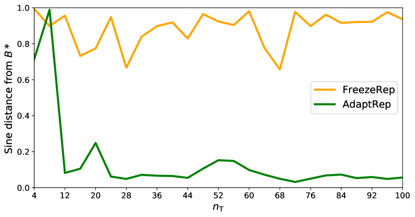
Figure 1: Sine distances of the representations learned by each method from the correct space $B^{\ast}$.

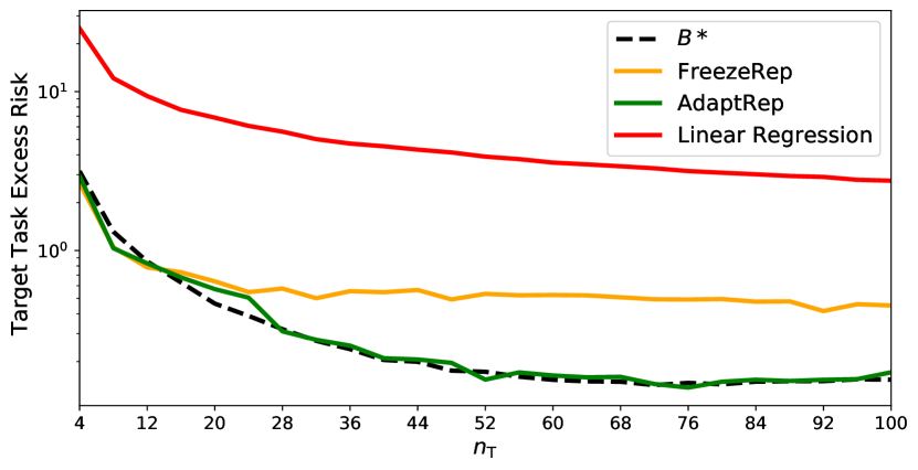
Figure 2: The average worst-case excess risk for several settings of $n_{\mathrm{T}}$, plotted on a logarithmic $y$-axis.

In this section, we experimentally verify the hard case for the linear setting presented in Section 3.4. Since the empirical success of MAML or its variants in general has already been demonstrated extensively in practice and in existing work, it is not the focus of this section.

Recall that in the hard case, we vary the amount of data $n_{\mathrm{T}}$ available to the learner during target time, and we set $d\asymp n_{\mathrm{T}}$. We fix $k=2$ throughout the experiment. The matrix $B^{\ast}$ spans the first $k$ coordinates, while the residuals $\delta_{t}^{\ast}$ lie in the span of the last $k$ coordinates. Finally, we set the $\sigma=2$ for the Gaussian noise.

During source training, both FrozenRep and AdaptRep are provided with $1000$ tasks and $10d$ samples per task from the task distribution in Section 3.4. During target time, we evaluate the learned representation on the worst-case regression task from the same family.

Before we detail our results, we briefly comment on the nonconvexity in the source training procedure. Rather than optimizing (4) or (7) during source training, we use an additional Frobenius-norm regularizer on $B^{\top}B-WW^{\top}$ to ensure that the two terms are balanced. In the case of FrozenRep, this regularized objective was shown to have a favorable optimization landscape in Tripuraneni et al. (2020a). We then used L-BFGS to optimize these regularized objectives. To further mitigate any possible optimization issues, we evaluated both methods with $10$ random restarts, and report the best of the $10$ restarts (as measured by the worst-case performance on the target task) for both methods.

(Subspace Alignment). First, we plot the alignment of the learned representation (using the best of the $10$ restarts described above) with the correct space $B^{\ast}$. We measure this via the sine of the largest principal angle between the two spaces, i.e.

$$\sin\Theta_{1}(\hat{B},B^{\ast})=\sqrt{1-\lambda_{1}^{2}\left(\hat{B}^{\top}B^{\ast}\right)}.$$

We plot the results in Figure 2. As predicted by Lemma 3.1, FrozenRep does not learn $B^{\ast}$, in contrast to AdaptRep.

(Target Task Performance). We proceeded to evaluate how the methods fare on their corresponding worst-case target tasks. We do so by training with the representation over $1000$ i.i.d. draws of the target dataset, and averaging the excess risk over all obtained representations. We provide the results in Figure 2, and include a comparison with standard linear regression as a baseline. As predicted, AdaptRep performs much better than FrozenRep, with a gap that grows with $n_{\mathrm{T}}$.

8 Conclusion

We have presented, to the best of our knowledge, the first statistical analysis of fine-tuning-based meta-learning. We demonstrate the success of such algorithms under the assumption of approximately shared representation between available tasks. In contrast, we show that methods analyzed by prior work that do not incorporate task-specific fine-tuning fail under this weaker assumption.

An interesting line of future work is to determine ways to formulate useful shared structure among MDPs, i.e. formulate settings for which meta-reinforcement learning succeeds and results in improved regret bounds for downstream tasks.

Appendix A Proof of Theorem 3.1

In this section, we will prove the performance guarantee in the linear representation setting presented in Theorem 3.1. We first compute a bound on the difference in the spans of the true underlying representation $B^{\ast}$ and the representation $B_{0}$ obtained from training on the source tasks. Having done so, we then analyze the performance of the best predictor found by projected gradient descent.

For clarity of presentation, we will write $\theta_{t}^{\ast}=B_{t}^{\ast}w_{t}^{\ast}+\delta_{t}^{\ast}$ and $\hat{\theta}_{t}=(B+\Delta_{t})w_{t}$ throughout this section. Furthermore, let $\hat{\delta}_{t}=\Delta_{t}w_{t}$. Finally, we will be making use of the following covariance concentration results throughout this section, allowing us to connect empirical averages to population averages and vice versa:

Lemma A.1 (Source covariance concentration, Du et al. (2020), Claim A.1).

If $n_{\mathrm{S}}\gg\rho^{4}[d+\log(T/\delta)]$, then with probability at least $1-\delta/9$ over the random draw of $n_{\mathrm{S}}T$ source inputs,

$$0.9\Sigma\preceq\frac{1}{n_{\mathrm{S}}}X_{t}^{\top}X_{t}\preceq 1.1\Sigma$$

for any $t\in[T]$.

Lemma A.2 (Target covariance concentration).

If $n_{\mathrm{T}}\gg\rho^{4}[d+\log(T/\delta)]$, then with probability at least $1-\delta/9$ over the random draw of $n_{\mathrm{T}}$ target inputs,

$$0.9\Sigma\preceq\frac{1}{n_{\mathrm{T}}}X^{\top}X\preceq 1.1\Sigma$$

for any $t\in[T]$.

Proof.

The proof is similar to that of Lemma A.1, and is omitted for brevity. ∎

A.1 Source Guarantees for the Linear Setting

We proceed to analyze the representation $B_{0}$ obtained from the source training procedure outlined in (4). Key to the analysis is a bound on the average population loss over the source tasks that the global minimizer of (4) can achieve as a function of $n_{\mathrm{S}}$:

Lemma A.3 (Source training bound).

Let $B_{0}$ be a minimizer of (4), and $\left\{(\Delta_{t},w_{t})\right\}_{t\in[T]}$ be minimizers for the inner optimization problem given $B_{0}$. If the regularizer coefficients are chosen such that

$$\lambda\asymp\frac{1}{T\delta_{0}}\left[\frac{\sigma\left\lVert\Sigma\right\rVert_{2}^{1/2}}{\sqrt{n_{\mathrm{S}}T}}\sqrt{kT+kd\log\kappa n_{\mathrm{S}}+\log\frac{1}{\delta}}+\frac{\sigma}{\sqrt{n_{\mathrm{S}}}}\sqrt{\operatorname{tr}{\Sigma}\left(1+\log\frac{T}{\delta}\right)}\right],$$

and $\gamma=\delta_{0}^{2}\lambda$, then with probability at least $1-\delta/3$,

$$\frac{1}{T}\sum_{t\in[T]}\left\lVert\Sigma^{1/2}(\theta_{t}^{\ast}-\hat{\theta}_{t})\right\rVert_{2}^{2}$$

$$\quad\lesssim\frac{\sigma^{2}}{n_{\mathrm{S}}T}\left(kT+kd\log\kappa n_{\mathrm{S}}+\log\frac{1}{\delta}\right)+\frac{\sigma\delta_{0}\left\lVert\Sigma\right\rVert_{2}^{1/2}}{\sqrt{n_{\mathrm{S}}T}}\sqrt{kT+kd\log\kappa n_{\mathrm{S}}+\log\frac{1}{\delta}}$$

$$\quad+\frac{\sigma\delta_{0}}{\sqrt{n_{\mathrm{S}}}}\sqrt{\operatorname{tr}{\Sigma}\left(1+\log\frac{T}{\delta}\right)}.$$

Proof.

Throughout this proof, we instantiate the high-probability event in Lemma A.1, which occurs with probability at least $1-\delta/9$.

Note that we can express $\delta_{t}^{\ast}$ as $[\delta_{t}^{\ast}(w_{t}^{\ast})^{\top}/\left\lVert w_{t}^{\ast}\right\rVert_{2}^{2}]w_{t}^{\ast}=\Delta_{t}^{\ast}w_{t}^{\ast}$. Thus, via the optimality of $B_{0}$ and $\left\{(\Delta_{t},w_{t})\right\}_{t\in[T]}$, we can form the basic inequality

$$\sum_{t\in[T]}\frac{1}{2n_{\mathrm{S}}T}\left\lVert y_{t}-X_{t}\hat{\theta}_{t}\right\rVert_{2}^{2}+\frac{\lambda}{2}\left\lVert\Delta_{t}\right\rVert_{F}^{2}+\frac{\gamma}{2}\left\lVert w_{t}\right\rVert_{2}^{2}$$

$$\qquad\leq\sum_{t\in[T]}\frac{1}{2n_{\mathrm{S}}T}\left\lVert z_{t}\right\rVert_{2}^{2}+\frac{\lambda}{2}\left\lVert\Delta_{t}^{\ast}\right\rVert_{F}^{2}+\frac{\gamma}{2}\left\lVert w_{t}^{\ast}\right\rVert_{2}^{2}$$

$$\qquad\leq\sum_{t\in[T]}\frac{1}{2n_{\mathrm{S}}T}\left\lVert z_{t}\right\rVert_{2}^{2}+\frac{\lambda}{2}\sum_{t\in[T]}\frac{\left\lVert\delta_{t}^{\ast}\right\rVert_{2}^{2}}{\left\lVert w_{t}^{\ast}\right\rVert_{2}^{2}}+\frac{\gamma}{2}\sum_{t\in[T]}\left\lVert w_{t}^{\ast}\right\rVert_{2}^{2}$$

$$\qquad\leq\sum_{t\in[T]}\frac{1}{2n_{\mathrm{S}}T}\left\lVert z_{t}\right\rVert_{2}^{2}+\left(\frac{\lambda\delta_{0}^{2}+\gamma}{2}\right)T$$

$$\qquad\leq\underbrace{\frac{\sigma\delta_{0}\left\lVert\Sigma\right\rVert_{2}^{1/2}}{\sqrt{nT}}\sqrt{kT+kd\log\kappa n_{\mathrm{S}}+\log\frac{1}{\delta}}+\frac{\sigma\delta_{0}}{\sqrt{n}}\sqrt{\operatorname{tr}\Sigma\left(1+\log\frac{T}{\delta}\right)}}_{\eqqcolon C_{n_{\mathrm{S}},T}}$$

$$\qquad\qquad+\sum_{t\in[T]}\frac{1}{2n_{\mathrm{S}}T}\left\lVert z_{t}\right\rVert_{2}^{2}.$$

Note that the simplification of the regularizer on the optimum holds since $\left\lVert w_{t}^{\ast}\right\rVert_{2}=\Theta(1)$ by Assumption 3.2. Equivalently, by rearranging,

$$\sum_{t\in[T]}\frac{1}{2n_{\mathrm{S}}T}\left\lVert X_{t}(\theta_{t}^{\ast}-\hat{\theta}_{t})\right\rVert_{2}^{2}+\frac{\lambda}{2}\left\lVert\Delta_{t}\right\rVert_{F}^{2}+\frac{\gamma}{2}\left\lVert w_{t}\right\rVert_{2}^{2}$$

$$\quad\leq\sum_{t\in[T]}\frac{1}{2n_{\mathrm{S}}T}\left\langle z_{t},X_{t}(\theta_{t}^{\ast}-\hat{\theta}_{t})\right\rangle+C_{n_{\mathrm{S}},T}.$$

Finally, by Proposition LABEL:prop:sum-regularizers-equivalence, the regularizer on $\Delta_{t}$ and $w_{t}$ can be rewritten as a regularizer on $\hat{\delta}_{t}$, i.e.

$$\sum_{t\in[T]}\frac{1}{2n_{\mathrm{S}}T}\left\lVert X_{t}(\theta_{t}^{\ast}-\hat{\theta}_{t})\right\rVert_{2}^{2}+\sqrt{\lambda\gamma}\left\lVert\hat{\delta}_{t}\right\rVert_{2}\leq\sum_{t\in[T]}\frac{1}{2n_{\mathrm{S}}T}\left\langle z_{t},X_{t}(\theta_{t}^{\ast}-\hat{\theta}_{t})\right\rangle+C_{n_{\mathrm{S}},T}.$$ (11)

To proceed, define the set $S$ as

$$\left\{[\alpha_{t}+\beta_{t}]_{t\in[T]}\ \middle|\ \operatorname{rank}{[\alpha_{t}]}\leq 2k,\left\lVert\beta_{t}\right\rVert_{2}\leq\delta_{0}+\left\lVert\hat{\delta}_{t}\right\rVert_{2},\left\lVert X_{t}(\alpha_{t}+\beta_{t})\right\rVert_{2}\leq\left\lVert X_{t}(\theta_{t}^{\ast}-\hat{\theta}_{t})\right\rVert_{2}\right\},$$

and observe that $[\theta_{t}^{\ast}-\hat{\theta}_{t}]_{t\in[T]}\in S$, by letting $\alpha_{t}=B^{\ast}w_{t}^{\ast}-B_{0}w_{t}$ and $\beta_{t}=\delta_{t}^{\ast}-\hat{\delta}_{t}$. We bound the right-hand side of (11) via bounding the supremum of the inner product over $S$, i.e.

$$\sum_{t\in[T]}\left\langle z_{t},X_{t}(\theta_{t}^{\ast}-\hat{\theta}_{t})\right\rangle\leq\sup_{[\alpha_{t}+\beta_{t}]\in S}\sum_{t\in[T]}\left\langle z_{t},X_{t}(\alpha_{t}+\beta_{t})\right\rangle.$$

Now, we decompose the Gaussian width as

$$\sup_{[\alpha_{t}+\beta_{t}]\in S}\sum_{t\in[T]}\left\langle z_{t},X_{t}(\alpha_{t}+\beta_{t})\right\rangle\leq\underbrace{\sup_{[\alpha_{t}]\in S}\sum_{t\in[T]}\left\langle z_{t},X_{t}\alpha_{t}\right\rangle}_{\text{(I)}}+\underbrace{\sup_{[\beta_{t}]\in S_{2}}\sum_{t\in[T]}\left\langle z_{t},X_{t}\beta_{t}\right\rangle}_{\text{(II)}},$$

where $S_{2}=\left\{[\beta_{t}]_{t\in[T]}\ \middle|\ \left\lVert\beta_{t}\right\rVert_{2}\leq\delta_{0}+\left\lVert\hat{\delta}_{t}\right\rVert_{2}\right\}$. Note the abuse of notation in (I), where we say $[\alpha_{t}]_{t\in[T]}\in S$ if there exists $[\beta_{t}]_{t\in[T]}$ so that $[\alpha_{t}+\beta_{t}]_{t\in[T]}\in S$. This decomposes the Gaussian width into the sum of the Gaussian widths of a low-rank set (I) and a small norm set (II). We proceed to bound both terms accordingly to these two properties.

Bounding the Gaussian width of the low-rank set (I).

To bound the Gaussian width, we first enlarge $S$ to remove $\beta_{t}$ from the definition of the feasible set. Fix any $(\alpha_{t},\beta_{t})$ pair satisfying the conditions in $S$, and note that

$$\left\lVert X_{t}\beta_{t}\right\rVert_{2}\lesssim\sqrt{n_{\mathrm{S}}}\left\lVert\Sigma\right\rVert_{2}^{1/2}\left(\delta_{0}+\left\lVert\hat{\delta}_{t}\right\rVert_{2}\right).$$

Therefore, by the reverse triangle inequality,

$$\left|\left\lVert X_{t}\alpha_{t}\right\rVert_{2}-\left\lVert X_{t}\beta_{t}\right\rVert_{2}\right|\leq\left\lVert X_{t}(\alpha_{t}+\beta_{t})\right\rVert_{2}$$

$$\qquad\implies\left\lVert X_{t}\alpha_{t}\right\rVert_{2}\leq\underbrace{\left\lVert X_{t}(\theta_{t}^{\ast}-\hat{\theta}_{t})\right\rVert_{2}+\sqrt{n_{\mathrm{S}}}\left\lVert\Sigma\right\rVert_{2}^{1/2}\left(\delta_{0}+\left\lVert\hat{\delta}_{t}\right\rVert_{2}\right)}_{\eqqcolon\rho_{t}}.$$

Consequently, we can enlarge the feasible set to

$$S_{1}\coloneqq\left\{[\alpha_{t}]\ \middle|\ \operatorname{rank}{[\alpha_{t}]}\leq 2k,\left\lVert X_{t}\alpha_{t}\right\rVert_{2}\leq\rho_{t}\right\}.$$

Having relaxed the constraints, we now proceed to the main argument.

Since $\operatorname{rank}{[\alpha_{t}]}\leq 2k$, there exists an orthogonal matrix $V\in\mathbb{R}^{d\times 2k}$ (dependent on $\alpha_{t}$) and vectors $r_{t}\in\mathbb{R}^{2k}$ such that $\alpha_{t}=Vr_{t}$. Therefore, the inner product in the Gaussian width would be unchanged if we project $z_{t}$ onto $X_{t}V$, i.e.

$$\sup_{[\alpha_{t}]\in S_{1}}\sum_{t\in[T]}\left\langle z_{t},X_{t}\alpha_{t}\right\rangle=\sup_{[\alpha_{t}]\in S_{1}}\sum_{t\in[T]}\left\langle P_{X_{t}V}z_{t},X_{t}Vr_{t}\right\rangle.$$

The key idea we will leverage is that if $V$ were chosen independently of $z_{t}$, then $P_{X_{t}V}z_{t}$ is Gaussian in a $2k$-dimensional space, and thus norm bounded by $\tilde{O}(\sqrt{2k})$ with high probability. However, due to the supremum over $\alpha_{t}$, this independence assumption is not satisfied. Nevertheless, we can obtain a fixed finite covering of the set of all rank-$2k$ matrices, and ensure that the aforementioned norm bound on $P_{X_{t}V}z_{t}$ holds for every $V$ in the covering via a union-bound. By choosing the discretization level of the covering appropriately, we can control the error resulting from approximating the supremum by some element of the covering.

Formally, let $\mathcal{O}^{d\times 2k}$ be the set of orthogonal matrices in $\mathbb{R}^{d\times 2k}$. By Proposition LABEL:prop:orth-mat-covering, there exists an $\varepsilon$-covering of $\mathcal{O}^{d\times 2k}$ in the Frobenius norm with at most $(6\sqrt{2k}/\varepsilon)^{2kd}$ elements. Let $\bar{V}$ be an element of the covering such that $\left\lVert V-\bar{V}\right\rVert_{F}\leq\varepsilon$. Then,

$$\left\langle z_{t},X_{t}\alpha_{t}\right\rangle =\left\langle z_{t},X_{t}\bar{V}r_{t}\right\rangle+\left\langle z_{t},X_{t}(V-\bar{V})r_{t}\right\rangle$$

$$\leq\left\lVert P_{X_{t}\bar{V}}z_{t}\right\rVert_{2}\left\lVert X_{t}\bar{V}r_{t}\right\rVert_{2}+\left\lVert z_{t}\right\rVert_{2}\left\lVert X_{t}(V-\bar{V})r_{t}\right\rVert_{2}$$

$$\leq\left\lVert P_{X_{t}\bar{V}}z_{t}\right\rVert_{2}\left\lVert X_{t}Vr_{t}\right\rVert_{2}+(\left\lVert P_{X_{t}\bar{V}}z_{t}\right\rVert_{2}+\left\lVert z_{t}\right\rVert_{2})\left\lVert X_{t}(V-\bar{V})r_{t}\right\rVert_{2}$$

$$\leq\left\lVert P_{X_{t}\bar{V}}z_{t}\right\rVert_{2}\left\lVert X_{t}Vr_{t}\right\rVert_{2}+(\left\lVert P_{X_{t}\bar{V}}z_{t}\right\rVert_{2}+\left\lVert z_{t}\right\rVert_{2})\left\lVert X_{t}(V-\bar{V})r_{t}\right\rVert_{2}$$

$$\lesssim\left\lVert P_{X_{t}\bar{V}}z_{t}\right\rVert_{2}\left\lVert X_{t}\alpha_{t}\right\rVert_{2}+\left\lVert z_{t}\right\rVert_{2}\left\lVert X_{t}(V-\bar{V})r_{t}\right\rVert_{2},$$

and thus

$$\sum_{t\in[T]}\left\langle z_{t},X_{t}Vr_{t}\right\rangle \leq\sqrt{\smash[b]{\underbrace{\left(\sum_{t\in[T]}\left\lVert P_{X_{t}\bar{V}}z_{t}\right\rVert_{2}^{2}\right)}_{(\text{A})}}\left(\sum_{t\in[T]}\left\lVert X_{t}\alpha_{t}\right\rVert_{2}^{2}\right)}\vphantom{\underbrace{\left(\sum_{t\in[T]}\right)}_{(A)}}$$

$$\quad+\sqrt{\smash[b]{\underbrace{\left(\sum_{t\in[T]}\left\lVert z_{t}\right\rVert_{2}^{2}\right)}_{(\text{B})}}\smash[b]{\underbrace{\left(\sum_{t\in[T]}\left\lVert X_{t}(V-\bar{V})r_{t}\right\rVert_{2}\right)}_{(\text{C})}}\vphantom{\left(\sum_{t\in[T]}\right)}}.\vphantom{\underbrace{\left(\sum_{t\in[T]}\right)}_{(A)}}$$

We will bound (A), (B), and (C) individually.

1. For a fixed $\bar{V}$, (A) is a chi-squared random variable with $kT$ degrees of freedom scaled by $\sigma^{2}$. However, since $\bar{V}$ depends on $V$, we need to have a high probability bound for any element of the covering. By using known concentration bounds for chi-squared random variables together with the union-bound, we find that uniformly over the covering,

   $$(\mathrm{A})\leq\sigma^{2}\left(kT+\log\frac{1}{\delta^{\prime}}\right)\qquad\text{w.p. $\geq 1-\delta^{\prime}\left(\frac{6\sqrt{2k}}{\varepsilon}\right)^{2kd}$}.$$

2. Note that (B) is a chi-squared random variable with $n_{\mathrm{S}}T$ degrees of freedom scaled by $\sigma^{2}$, and thus

   $$(\mathrm{B})\lesssim\sigma^{2}\left(n_{\mathrm{S}}T+\log\frac{1}{\delta}\right)\qquad\text{w.p. $\geq 1-\frac{\delta}{18}$}.$$

3. Since $(1/n_{\mathrm{S}})X^{\top}X$ is concentrated about $\Sigma$ via Lemma A.1,

   $$\left\lVert X_{t}(V-\bar{V})r_{t}\right\rVert_{2}^{2} \lesssim n_{\mathrm{S}}\left\lVert\Sigma\right\rVert_{2}\varepsilon^{2}\left\lVert r_{t}\right\rVert_{2}^{2}=n_{\mathrm{S}}\left\lVert\Sigma\right\rVert_{2}\varepsilon^{2}\left\lVert Vr_{t}\right\rVert_{2}^{2}\lesssim\kappa\varepsilon^{2}\left\lVert X_{t}Vr_{t}\right\rVert_{2}^{2}.$$

Putting these bounds together, and setting $\varepsilon=\sqrt{k/\kappa n_{\mathrm{S}}}$ and $\delta^{\prime}=\delta/[18(6\sqrt{2k}/\varepsilon)^{2kd}]$, we obtain

$$\sum_{t\in[T]}\left\langle z_{t},X_{t}\alpha_{t}\right\rangle \lesssim\left(\sigma\sqrt{kT+\log\frac{1}{\delta^{\prime}}}+\varepsilon\sigma\sqrt{\kappa n_{\mathrm{S}}T+\log\frac{1}{\delta}}\right)\sqrt{\left(\sum_{t\in[T]}\left\lVert X_{t}Vr_{t}\right\rVert_{2}^{2}\right)}$$

$$\lesssim\left(\sigma\sqrt{kT+\log\frac{1}{\delta^{\prime}}}\right)\sqrt{\left(\sum_{t\in[T]}\left\lVert X_{t}Vr_{t}\right\rVert_{2}^{2}\right)}\qquad\qquad(k<n_{\mathrm{S}},\delta^{\prime}<\delta)$$

$$\lesssim\sigma\sqrt{kT+kd\log\kappa n_{\mathrm{S}}+\log\frac{1}{\delta}}\sqrt{\left(\sum_{t\in[T]}\left\lVert X_{t}\alpha_{t}\right\rVert_{2}^{2}\right)}.$$

Taking the supremum over $S_{1}$, we thus obtain the following bound on the Gaussian width:

$$\sup_{[\alpha_{t}]\in S_{1}}\sum_{t\in[T]}\left\langle z_{t},X_{t}\alpha_{t}\right\rangle$$

$$\quad\lesssim\sigma\sqrt{kT+kd\log\kappa n_{\mathrm{S}}+\log\frac{1}{\delta}}\left[\sqrt{\sum_{t\in[T]}\left\lVert X_{t}(\theta_{t}^{\ast}-\hat{\theta}_{t})\right\rVert_{2}^{2}\vphantom{\sum^{T}}}+\sqrt{\left\lVert\Sigma\right\rVert_{2}n_{\mathrm{S}}T}\left(\delta_{0}+\left\lVert\hat{\delta}_{t}\right\rVert_{2}\right)\right].$$

Note that the events for this sub-argument occur with probability at least $1-\delta/9$.

Bounding the Gaussian width of the low-norm set (II).

Recall that we want to bound

$$\sup_{[\beta_{t}]\in S_{2}}\sum_{t\in[T]}\left\langle z_{t},X_{t}\beta_{t}\right\rangle,\quad S_{2}\coloneqq\left\{[\beta_{t}]\ \middle|\ \left\lVert\beta_{t}\right\rVert_{2}\leq\delta_{0}+\left\lVert\hat{\delta}_{t}\right\rVert_{2}\right\}.$$

For any $t\in[T]$,

$$\left\langle z_{t},X_{t}\beta_{t}\right\rangle=\left\langle X_{t}^{\top}z_{t},\beta_{t}\right\rangle\leq\left(\delta_{0}+\left\lVert\hat{\delta}_{t}\right\rVert_{2}\right)\left\lVert X_{t}^{\top}z_{t}\right\rVert_{2}.$$

Furthermore, by the Hanson-Wright inequality, we have that with probability at least $1-\delta/9T$,

$$\left\lVert X_{t}^{\top}z_{t}\right\rVert_{2}\lesssim\sigma\sqrt{n_{\mathrm{S}}\operatorname{tr}\Sigma\left(1+\log\frac{T}{\delta}\right)}.$$

Putting everything together, we thus find that with probability at least $1-\delta/9$,

$$\sup_{[\beta_{t}]\in S_{2}}\sum_{t\in[T]}\left\langle z_{t},X_{t}\beta_{t}\right\rangle\leq\sigma\left(T\delta_{0}+\sum_{t\in[T]}\left\lVert\hat{\delta}_{t}\right\rVert_{2}\right)\sqrt{n_{\mathrm{S}}\operatorname{tr}\Sigma\left(1+\log\frac{T}{\delta}\right)}.$$

Combining the bounds and concluding.

Having bounded both Gaussian widths, we can thus bound the right-hand side of (11) as

$$\sum_{t\in[T]}\frac{1}{2n_{\mathrm{S}}T}\left\lVert X_{t}(\theta_{t}^{\ast}-\hat{\theta}_{t})\right\rVert_{2}^{2}+\left(\sqrt{\lambda\gamma}-\frac{1}{\delta_{0}T}C_{n_{\mathrm{S}},T}\right)\left\lVert\hat{\delta}_{t}\right\rVert_{2}$$

$$\quad\lesssim\frac{\sigma}{\sqrt{nT}}\sqrt{kT+kd\log\kappa n_{\mathrm{S}}+\log\frac{1}{\delta}}\left(\sum_{t\in[T]}\frac{1}{2n_{\mathrm{S}}T}\left\lVert X_{t}(\theta_{t}^{\ast}-\hat{\theta}_{t})\right\rVert_{2}^{2}\right)^{1/2}+C_{n_{\mathrm{S}},T}.$$

Therefore, as long as $\sqrt{\lambda\gamma}\geq(1/\delta_{0}T)C_{n_{\mathrm{S}},T}$,

$$\sum_{t\in[T]}\frac{1}{2n_{\mathrm{S}}T}\left\lVert X_{t}(\theta_{t}^{\ast}-\hat{\theta}_{t})\right\rVert_{2}^{2}$$

$$\quad\lesssim\frac{\sigma}{\sqrt{n_{\mathrm{S}}T}}\sqrt{kT+kd\log\kappa n_{\mathrm{S}}+\log\frac{1}{\delta}}\left(\sum_{t\in[T]}\frac{1}{2n_{\mathrm{S}}T}\left\lVert X_{t}(\theta_{t}^{\ast}-\hat{\theta}_{t})\right\rVert_{2}^{2}\right)^{1/2}+C_{n_{\mathrm{S}},T}.$$

Finally, by solving the quadratic inequality using Proposition LABEL:prop:solve-quad-ineqs, we find that

$$\sum_{t\in[T]}\frac{1}{2n_{\mathrm{S}}T}\left\lVert X_{t}(\theta_{t}^{\ast}-\hat{\theta}_{t})\right\rVert_{2}^{2}$$

$$\quad\lesssim\frac{\sigma^{2}}{n_{\mathrm{S}}T}\left(kT+kd\log\kappa n_{\mathrm{S}}+\log\frac{1}{\delta}\right)+\frac{\sigma\delta_{0}\left\lVert\Sigma\right\rVert_{2}^{1/2}}{\sqrt{n_{\mathrm{S}}T}}\sqrt{kT+kd\log\kappa n_{\mathrm{S}}+\log\frac{1}{\delta}}$$

$$\qquad\qquad+\frac{\sigma\delta_{0}}{\sqrt{n_{\mathrm{S}}}}\sqrt{\operatorname{tr}{\Sigma}\left(1+\log\frac{T}{\delta}\right)},$$

from which the desired performance bound follows due to the concentration of the empirical covariance from Lemma A.1. Since the concentration of the source covariance matrices and each of the sub-arguments all hold with probability at least $1-\delta/9$, it follows that the main claim holds with probability at least $1-\delta/3$. ∎

The prior bound is central to the analysis, as the performance of the learner can be tied to how well $B_{0}$ spans the correct space. To see why this is the case, note that for large $n_{\mathrm{S}}$, the effect of the noise on the optimization in (4) is negligible. In this regime, no matter which representation $B_{0}$ the learner has chosen, the optimal predictor would satisfy $P_{X_{t}B_{0}}X_{t}\hat{\theta}_{t}\approx P_{X_{t}B_{0}}X_{t}\theta_{t}^{\ast}$ and $P_{X_{t}B_{0}}^{\perp}X_{t}\hat{\theta}_{t}\approx P_{X_{t}B_{0}}^{\perp}X_{t}\theta_{t}^{\ast}$. Consequently, the performance of the predictors chosen by the learner can be tied to the chosen representation $B_{0}$. We formalize this intuition in the following result:

Lemma A.4 (Transfer Lemma).

Under Assumption 3.2, we have that

$$\left\lVert P_{\Sigma^{1/2}B_{0}}\Sigma^{1/2}B^{\ast}\right\rVert_{F}^{2}\lesssim k\left[\frac{1}{T}\sum_{t\in[T]}\left\lVert\Sigma^{1/2}(\theta_{t}^{\ast}-\hat{\theta}_{t})\right\rVert_{2}^{2}\right].$$

Proof.

Throughout this proof, we will write $P\coloneqq P_{\Sigma^{1/2}B_{0}}$ and $P^{\perp}\coloneqq P_{\Sigma^{1/2}B_{0}}^{\perp}$ for readability. To proceed, note that we intuitively expect that for a learner that has learned the correct spaces, $P\Sigma^{1/2}\hat{\theta}_{t}\approx\Sigma^{1/2}B^{\ast}w_{t}^{\ast}$ as it is the low-rank component of the estimator, and consequently, $P^{\perp}\Sigma^{1/2}\hat{\theta}_{t}\approx\Sigma^{1/2}\delta_{t}^{\ast}$. Then, decomposing into the corresponding errors, we have that for any $t\in[T]$,

$$\left\lVert\Sigma^{1/2}(\theta_{t}^{\ast}-\hat{\theta}_{t})\right\rVert_{2}^{2} \gtrsim\left\lVert\Sigma^{1/2}B^{\ast}w_{t}^{\ast}-P\Sigma^{1/2}\hat{\theta}_{t}\right\rVert_{2}^{2}+\left\lVert\Sigma^{1/2}\delta_{t}^{\ast}-P^{\perp}\Sigma^{1/2}\hat{\theta}_{t}\right\rVert_{2}^{2}$$

$$\qquad+2\left\langle\Sigma^{1/2}B^{\ast}w_{t}^{\ast}-P\Sigma^{1/2}\hat{\theta}_{t},\Sigma^{1/2}\delta_{t}^{\ast}-P^{\perp}\Sigma^{1/2}\hat{\theta}_{t}\right\rangle$$

$$\geq\left\lVert P^{\perp}\Sigma^{1/2}B^{\ast}w_{t}^{\ast}\right\rVert_{2}^{2}+\left\lVert\Sigma^{1/2}\delta_{t}^{\ast}-P^{\perp}\Sigma^{1/2}\hat{\theta}_{t}\right\rVert_{2}^{2}$$

$$\qquad-2\left|\left\langle\Sigma^{1/2}B^{\ast}w_{t}^{\ast}-P\Sigma^{1/2}\hat{\theta}_{t},\Sigma^{1/2}\delta_{t}^{\ast}-P^{\perp}\Sigma^{1/2}\hat{\theta}_{t}\right\rangle\right|.$$

We proceed to bound the inner product above. We do so by observing that if we were to replace $\hat{\theta}_{t}$ by $\theta_{t}^{\ast}$, then

$$\left\langle\Sigma^{1/2}B^{\ast}w_{t}^{\ast}-P\Sigma^{1/2}\theta_{t}^{\ast},\Sigma^{1/2}\delta_{t}^{\ast}-P^{\perp}\Sigma^{1/2}\delta_{t}^{\ast}\right\rangle$$

$$\qquad=\left\langle P^{\perp}\Sigma^{1/2}B^{\ast}w_{t}^{\ast}-P\Sigma^{1/2}\delta_{t}^{\ast},P^{\perp}\Sigma^{1/2}\delta_{t}^{\ast}-P\Sigma^{1/2}B^{\ast}w_{t}^{\ast}\right\rangle$$

$$\qquad=(w_{t}^{\ast})^{\top}(B^{\ast})^{\top}\Sigma\delta_{t}^{\ast}$$

$$\qquad=0.$$

To translate this result into a bound on the original inner product, we note that as $n_{\mathrm{S}}\to\infty$, and the impact of the noise and the regularizer on the optimization is diminished, we expect $\hat{\theta}_{t}$ to learn the projections of $X_{t}\theta_{t}^{\ast}$ onto $X_{t}B_{0}$ and its complement. With these two insights in mind, we decompose the inner product as

$$\left|\left\langle\Sigma^{1/2}B^{\ast}w_{t}^{\ast}-P\Sigma^{1/2}\hat{\theta}_{t},\Sigma^{1/2}\delta_{t}^{\ast}-P^{\perp}\Sigma^{1/2}\hat{\theta}_{t}\right\rangle\right|$$

$$\quad\leq\left|\left\langle\Sigma^{1/2}B^{\ast}w_{t}^{\ast}-P\Sigma^{1/2}\theta_{t}^{\ast},P^{\perp}\Sigma^{1/2}(\theta_{t}^{\ast}-\hat{\theta}_{t})\right\rangle\right|$$

$$\qquad\quad+\left|\left\langle P\Sigma^{1/2}(\theta_{t}^{\ast}-\hat{\theta}_{t}),\Sigma^{1/2}\delta_{t}^{\ast}-P^{\perp}\Sigma^{1/2}\hat{\theta}_{t}\right\rangle\right|$$

$$\qquad\quad+\underbrace{\left|\left\langle\Sigma^{1/2}B^{\ast}w_{t}^{\ast}-P\Sigma^{1/2}\theta_{t}^{\ast},\Sigma^{1/2}\delta_{t}^{\ast}-P^{\perp}\Sigma^{1/2}\theta_{t}^{\ast}\right\rangle\right|}_{=0}$$

$$\quad=\left|\left\langle P^{\perp}\Sigma^{1/2}B^{\ast}w_{t}^{\ast},P^{\perp}\Sigma^{1/2}(\theta_{t}^{\ast}-\hat{\theta}_{t})\right\rangle\right|+\left|\left\langle P\Sigma^{1/2}(\theta_{t}^{\ast}-\hat{\theta}_{t}),\Sigma^{1/2}\delta_{t}^{\ast}-P^{\perp}\Sigma^{1/2}\hat{\theta}_{t}\right\rangle\right|.$$

Putting everything together, we find that

$$\frac{1}{T}\sum_{t\in[T]}\left\lVert P^{\perp}\Sigma^{1/2}B^{\ast}w_{t}^{\ast}\right\rVert_{2}^{2}+\frac{1}{T}\sum_{t\in[T]}\left\lVert\Sigma^{1/2}\delta_{t}^{\ast}-P^{\perp}\Sigma^{1/2}\hat{\theta}_{t}\right\rVert_{2}^{2}$$

$$\qquad\lesssim\frac{1}{T}\sum_{t\in[T]}\left\lVert\Sigma^{1/2}(\theta_{t}^{\ast}-\hat{\theta}_{t})\right\rVert_{2}^{2}+\frac{1}{T}\sum_{t\in[T]}\left|\left\langle\Sigma^{1/2}B^{\ast}w_{t}^{\ast}-P\Sigma^{1/2}\hat{\theta}_{t},\Sigma^{1/2}\delta_{t}^{\ast}-P^{\perp}\Sigma^{1/2}\hat{\theta}_{t}\right\rangle\right|$$

$$\qquad\leq\frac{1}{T}\sum_{t\in[T]}\left\lVert\Sigma^{1/2}(\theta_{t}^{\ast}-\hat{\theta}_{t})\right\rVert_{2}^{2}+\frac{1}{T}\sum_{t\in[T]}\left|\left\langle P^{\perp}\Sigma^{1/2}B^{\ast}w_{t}^{\ast},P^{\perp}\Sigma^{1/2}(\theta_{t}^{\ast}-\hat{\theta}_{t})\right\rangle\right|$$

$$\qquad\qquad+\frac{1}{T}\sum_{t\in[T]}\left|\left\langle P\Sigma^{1/2}(\theta_{t}^{\ast}-\hat{\theta}_{t}),\Sigma^{1/2}\delta_{t}^{\ast}-P^{\perp}\Sigma^{1/2}\hat{\theta}_{t}\right\rangle\right|$$

$$\qquad\leq\frac{1}{T}\sum_{t\in[T]}\left\lVert\Sigma^{1/2}(\theta_{t}^{\ast}-\hat{\theta}_{t})\right\rVert_{2}^{2}+\sqrt{\frac{1}{T}\sum_{t\in[T]}\left\lVert P^{\perp}\Sigma^{1/2}(\theta_{t}^{\ast}-\hat{\theta}_{t})\right\rVert_{2}^{2}\vphantom{\sum^{T}}}\sqrt{\frac{1}{T}\sum_{t\in[T]}\left\lVert P^{\perp}\Sigma^{1/2}B^{\ast}w_{t}^{\ast}\right\rVert_{2}^{2}\vphantom{\sum^{T}}}$$

$$\qquad\qquad+\sqrt{\frac{1}{T}\sum_{t\in[T]}\left\lVert P\Sigma^{1/2}(\theta_{t}^{\ast}-\hat{\theta}_{t})\right\rVert_{2}^{2}\vphantom{\sum^{T}}}\sqrt{\frac{1}{T}\sum_{t\in[T]}\left\lVert\Sigma^{1/2}\delta_{t}^{\ast}-P^{\perp}\Sigma^{1/2}\hat{\theta}_{t}\right\rVert_{2}^{2}\vphantom{\sum^{T}}}.$$

This is a quadratic inequality in the two terms on the left-hand side, and so by applying Proposition LABEL:prop:solve-quad-ineqs,

$$\frac{1}{T}\sum_{t\in[T]}\left\lVert P^{\perp}\Sigma^{1/2}B^{\ast}w_{t}^{\ast}\right\rVert_{2}^{2} \lesssim\frac{1}{T}\sum_{t\in[T]}\left\lVert P^{\perp}\Sigma^{1/2}(\theta_{t}^{\ast}-\hat{\theta}_{t})\right\rVert_{2}^{2}+\frac{1}{T}\sum_{t\in[T]}\left\lVert P\Sigma^{1/2}(\theta_{t}^{\ast}-\hat{\theta}_{t})\right\rVert_{2}^{2}$$

$$\qquad+\frac{1}{T}\sum_{t\in[T]}\left\lVert\Sigma^{1/2}(\theta_{t}^{\ast}-\hat{\theta}_{t})\right\rVert_{2}^{2}$$

$$\lesssim\frac{1}{T}\sum_{t\in[T]}\left\lVert\Sigma^{1/2}(\theta_{t}^{\ast}-\hat{\theta}_{t})\right\rVert_{2}^{2},$$

where the last line follows by orthogonality. Finally, by Proposition LABEL:prop:mat-to-proj,

$$\frac{1}{T}\sum_{t\in[T]}\left\lVert P^{\perp}\Sigma^{1/2}B^{\ast}w_{t}^{\ast}\right\rVert_{2}^{2}=\frac{1}{T}\left\lVert P^{\perp}\Sigma^{1/2}B^{\ast}W^{\ast}\right\rVert_{F}^{2}\geq\frac{\sigma_{k}(W^{\ast})^{2}}{T}\left\lVert P_{\Sigma^{1/2}B_{0}}^{\perp}\Sigma^{1/2}B^{\ast}\right\rVert_{F}^{2},$$

which together with the diversity assumption in Assumption 3.2 yields the final bound

$$\left\lVert P_{\Sigma^{1/2}B_{0}}^{\perp}\Sigma^{1/2}B^{\ast}\right\rVert_{F}^{2}\lesssim k\left[\frac{1}{T}\sum_{t\in[T]}\left\lVert\Sigma^{1/2}(\theta_{t}^{\ast}-\hat{\theta}_{t})\right\rVert_{2}^{2}\right].\qed$$

A.2 Target Guarantees for the Linear Setting

Having established a connection between the performance on the source tasks and the difference in the spans of $B^{\ast}$ and $B_{0}$, we can now analyze the performance of the target training procedure. First, we bound the performance of nearly optimal points in $\mathcal{C}_{\beta}$ for several possible choices of $c_{1},c_{2}$.

Lemma A.5 (Statistical Rates for $\mathcal{L}_{\beta}$).

Assume that $(\Delta,w)$ is $\zeta$-suboptimal for $\mathcal{L}_{\beta}$ with the constraint set $\mathcal{C}_{\beta}=\left\{(\Delta,w)\ \middle|\ \left\lVert\Delta\right\rVert_{F}\leq c_{1}/\beta,\left\lVert w\right\rVert_{2}\leq c_{2}/\beta\right\}$, i.e.

$$\mathcal{L}_{\beta}(\Delta,w)\leq\min_{(\Delta^{\prime},w^{\prime})\in\mathcal{C}_{\beta}}\mathcal{L}_{\beta}(\Delta^{\prime},w^{\prime})+\zeta.$$

We write $\hat{\theta}$ for the predictor corresponding to $(\Delta,w)$, i.e. $\hat{\theta}=\beta(A_{B_{0}}+\Delta)(w_{0}+w)$. Now, let

$$\bar{w} =(B_{0}X^{\top}XB_{0})^{\dagger}B_{0}^{\top}X^{\top}X\theta^{\ast}$$

$$\bar{\delta} =\theta^{\ast}-B_{0}\bar{w}$$

$$\tilde{w} =(B_{0}^{\top}X^{\top}XB_{0})^{\dagger}B_{0}^{\top}X^{\top}XB^{\ast}w^{\ast}.$$

Note that $XB_{0}\bar{w}=P_{XB_{0}}X\theta^{\ast}$, $X\bar{\delta}=P_{XB_{0}}^{\perp}X\theta^{\ast}$, and $XB\tilde{w}=P_{XB_{0}}XB^{\ast}w^{\ast}$. Then, assuming $\beta>\max(\left\lVert\bar{w}\right\rVert_{2},\left\lVert\tilde{w}\right\rVert_{2})$,

$$\frac{1}{2n_{\mathrm{T}}}\left\lVert X(\theta^{\ast}-\hat{\theta})\right\rVert_{2}^{2}\lesssim\zeta+\begin{cases}\!\begin{aligned} &\left\lVert P_{\Sigma^{1/2}B_{0}}^{\perp}\Sigma^{1/2}B^{\ast}w^{\ast}\right\rVert_{2}^{2}\\ &\qquad+\frac{\sigma^{2}}{n_{\mathrm{T}}}\left(k+\log\frac{1}{\delta}\right)\\ &\qquad+\frac{\sigma\delta_{0}}{\sqrt{n_{\mathrm{T}}}}\sqrt{\operatorname{tr}\Sigma\left(1+\log\frac{1}{\delta}\right)}\end{aligned}&c_{1}=\delta_{0},c_{2}=\left\lVert\tilde{w}\right\rVert_{2}\\[38.74988pt] \!\begin{aligned} &\frac{\sigma^{2}}{n_{\mathrm{T}}}\left(k+\log\frac{1}{\delta}\right)\\ &\qquad+\frac{\sigma\left\lVert\bar{\delta}\right\rVert_{2}}{\sqrt{n_{\mathrm{T}}}}\sqrt{\operatorname{tr}\Sigma\left(1+\log\frac{1}{\delta}\right)}\end{aligned}&c_{1}=\left\lVert\bar{\delta}\right\rVert_{2},c_{2}=\left\lVert\bar{w}\right\rVert_{2}\\[30.1388pt] \displaystyle\frac{\sigma^{2}}{n_{\mathrm{T}}}\left(d+\log\frac{1}{\delta}\right)&c_{1}=\left\lVert\theta^{\ast}\right\rVert_{2},c_{2}=0\end{cases}$$

with probability at least $1-\delta/3$.

Proof.

We proceed by proving the three cases separately. Throughout the proof, we instantiate the high-probability event in Lemma A.2, which guarantees that

$$0.9\Sigma\preceq\frac{1}{n_{\mathrm{T}}}X^{\top}X\preceq 1.1\Sigma.$$

Recall that this event occurs with probability at least $1-\delta/9$.

$c_{1}=\delta_{0},c_{2}=\left\lVert\tilde{w}\right\rVert_{2}$

Due to the choice of $c_{1}$ and $c_{2}$, there exists a parameter in $\mathcal{C}_{\beta}$ corresponding to the prediction vector $P_{XB_{0}}X\theta^{\ast}+X\delta^{\ast}$. Writing the corresponding basic inequality, we thus have that

$$\frac{1}{2n_{\mathrm{T}}}\left\lVert y-X\hat{\theta}\right\rVert_{2}^{2}-\zeta\leq\frac{1}{2n_{\mathrm{T}}}\left\lVert P_{XB_{0}}^{\perp}XB^{\ast}w^{\ast}\right\rVert_{2}^{2}+\frac{1}{n_{\mathrm{T}}}\left\langle z,P_{XB_{0}}^{\perp}XB^{\ast}w^{\ast}\right\rangle+\frac{1}{2n_{\mathrm{T}}}\left\lVert z\right\rVert_{2}^{2}$$

$$\qquad\implies\frac{1}{2n_{\mathrm{T}}}\left\lVert X(\theta^{\ast}-\hat{\theta})\right\rVert_{2}^{2}\leq\zeta+\frac{1}{2n_{\mathrm{T}}}\left\lVert P_{XB_{0}}^{\perp}XB^{\ast}w^{\ast}\right\rVert_{2}^{2}+\frac{1}{n_{\mathrm{T}}}\left\langle z,P_{XB_{0}}^{\perp}XB^{\ast}w^{\ast}\right\rangle$$

$$\qquad\qquad\qquad\qquad\qquad\qquad\qquad-\frac{1}{n_{\mathrm{T}}}\left\langle z,X(\theta^{\ast}-\hat{\theta})\right\rangle.$$

Simplifying further,

$$\frac{1}{n_{\mathrm{T}}}\left\langle z,P_{XB_{0}}^{\perp}XB^{\ast}w^{\ast}\right\rangle-\frac{1}{n_{\mathrm{T}}}\left\langle z,X(\theta^{\ast}-\hat{\theta})\right\rangle$$

$$\qquad=\frac{1}{n_{\mathrm{T}}}\left\langle z,P_{XB_{0}}X(\hat{\theta}-\theta^{\ast})\right\rangle-\frac{1}{n_{\mathrm{T}}}\left\langle z,P_{XB_{0}}^{\perp}X(\delta^{\ast}-\beta\Delta(w_{0}+w))\right\rangle.$$

Now, by the Hanson-Wright inequality, we can bound the last term as

$$-\frac{1}{n_{\mathrm{T}}}\left\langle X^{\top}P_{XB_{0}}^{\perp}z,\delta^{\ast}-\beta\Delta(w_{0}+w)\right\rangle \leq\frac{1}{n_{\mathrm{T}}}\left\lVert X^{\top}P_{XB_{0}}^{\perp}z\right\rVert_{2}\left\lVert\delta^{\ast}+\beta\Delta(w_{0}+w)\right\rVert_{2}$$

$$\lesssim\frac{\sigma\delta_{0}}{\sqrt{n_{\mathrm{T}}}}\sqrt{\operatorname{tr}\Sigma\left(1+\log\frac{1}{\delta}\right)}$$

with probability at least $1-\delta/9$. Therefore, we can rewrite the prior basic inequality as

$$\frac{1}{2n_{\mathrm{T}}}\left\lVert X(\theta^{\ast}-\hat{\theta})\right\rVert_{2}^{2} \lesssim\underbrace{\frac{1}{2n_{\mathrm{T}}}\left\lVert P_{XB_{0}}^{\perp}XB^{\ast}w^{\ast}\right\rVert_{2}^{2}+\frac{\sigma\delta_{0}}{\sqrt{n_{\mathrm{T}}}}\sqrt{\operatorname{tr}\Sigma\left(1+\log\frac{1}{\delta}\right)}+\zeta}_{\eqqcolon C}$$

$$\qquad+\frac{1}{n_{\mathrm{T}}}\left\langle z,P_{XB_{0}}X(\theta^{\ast}-\hat{\theta})\right\rangle.$$

Now, note that we can form the quadratic inequality

$$\frac{1}{n_{\mathrm{T}}}\left\lVert P_{XB_{0}}X(\theta^{\ast}-\hat{\theta})\right\rVert_{2}^{2}\leq\frac{1}{n_{\mathrm{T}}}\left\lVert P_{XB_{0}}z\right\rVert_{2}\left\lVert P_{XB_{0}}X(\theta^{\ast}-\hat{\theta})\right\rVert_{2}+C,$$

and thus by applying Proposition LABEL:prop:solve-quad-ineqs to solve the inequality and noting that $P_{XB_{0}}z/\sigma$ is distributed as a chi-squared random variable with $k$ degrees of freedom,

$$\frac{1}{n_{\mathrm{T}}}\left\lVert X(\theta^{\ast}-\hat{\theta})\right\rVert_{2}^{2} \lesssim\zeta+\left\lVert P_{\Sigma^{1/2}B_{0}}^{\perp}\Sigma^{1/2}B^{\ast}w^{\ast}\right\rVert_{2}^{2}$$

$$\qquad+\frac{\sigma^{2}}{n_{\mathrm{T}}}\left(k+\log\frac{1}{\delta}\right)+\frac{\sigma\delta_{0}}{\sqrt{n_{\mathrm{T}}}}\sqrt{\operatorname{tr}\Sigma\left(1+\log\frac{1}{\delta}\right)}$$

with probability at least $1-\delta/9$, which is the bound that we wanted to show.

$c_{1}=\left\lVert\bar{\delta}\right\rVert_{2},c_{2}=\left\lVert\bar{w}\right\rVert_{2}$

Due to the choice of $c_{1}$ and $c_{2}$, there exists a parameter in $\mathcal{C}_{\beta}$ corresponding to a predictor that agrees with $\theta^{\ast}$ on the target samples. Therefore,

$$\frac{1}{2n_{\mathrm{T}}}\left\lVert X(\theta^{\ast}-\hat{\theta})\right\rVert_{2}^{2}\leq\zeta+\frac{1}{2n_{\mathrm{T}}}\left\lVert z\right\rVert_{2}^{2}$$

$$\qquad\implies\frac{1}{2n_{\mathrm{T}}}\left\lVert X(\theta^{\ast}-\hat{\theta})\right\rVert_{2}^{2}\leq\zeta+\frac{1}{n_{\mathrm{T}}}\left\langle z,P_{XB_{0}}X(\theta^{\ast}-\hat{\theta})\right\rangle+\frac{1}{n_{\mathrm{T}}}\left\langle z,P_{XB_{0}}^{\perp}X(\theta^{\ast}-\hat{\theta})\right\rangle.$$ (12)

We proceed with an argument similar to that used in the source guarantee, albeit simpler since the representation $B_{0}$ is fixed (and thus no covering argument is required). Along these lines, we bound the first term using the low-rank of $B_{0}$. Via projections,

$$\frac{1}{n_{\mathrm{T}}}\left\lVert P_{XB_{0}}X(\theta^{\ast}-\hat{\theta})\right\rVert_{2}^{2}$$

$$\qquad\lesssim\zeta+\frac{1}{n_{\mathrm{T}}}\left\lVert P_{XB_{0}}z\right\rVert_{2}\left\lVert P_{XB_{0}}X(\theta^{\ast}-\hat{\theta})\right\rVert_{2}+\frac{1}{n_{\mathrm{T}}}\left\langle z,P_{XB_{0}}^{\perp}X(\theta^{\ast}-\hat{\theta})\right\rangle.$$

Therefore, by applying Proposition LABEL:prop:solve-quad-ineqs to solve the quadratic inequality, we have that with probability at least $1-\delta/9$,

$$\frac{1}{2n_{\mathrm{T}}}\left\lVert X(\theta^{\ast}-\hat{\theta})\right\rVert_{2}^{2}\leq\zeta+\frac{\sigma^{2}}{n_{\mathrm{T}}}\left(k+\log\frac{1}{\delta}\right)+\frac{1}{n_{\mathrm{T}}}\left\langle z,P_{XB_{0}}^{\perp}X(\theta^{\ast}-\hat{\theta})\right\rangle.$$

To bound the second term, we simply make use of the norm constraints defining the feasible set $\mathcal{C}_{\beta}$, which we note is analogous to the low-norm sub-argument of the source guarantee. Formally, the Hanson-Wright inequality implies that with probability at least $1-\delta/9$,

$$\frac{1}{n_{\mathrm{T}}}\left\langle z,P_{XB_{0}}^{\perp}X(\theta^{\ast}-\hat{\theta})\right\rangle =\frac{1}{\sqrt{n_{\mathrm{T}}}}\left\lVert\frac{1}{\sqrt{n_{\mathrm{T}}}}X^{\top}P_{XB_{0}}^{\perp}z\right\rVert_{2}\left\lVert\bar{\delta}+\beta\Delta w_{0}+\beta\Delta w\right\rVert_{2}$$

$$\lesssim\frac{\sigma\left\lVert\bar{\delta}\right\rVert_{2}}{\sqrt{n_{\mathrm{T}}}}\sqrt{\operatorname{tr}\Sigma\left(1+\log\frac{1}{\delta}\right)}.$$

Putting everything together, we thus have that

$$\frac{1}{2n_{\mathrm{T}}}\left\lVert X(\theta^{\ast}-\hat{\theta})\right\rVert_{2}^{2}\lesssim\zeta+\frac{\sigma^{2}}{n_{\mathrm{T}}}\left(k+\log\frac{1}{\delta}\right)+\frac{\sigma\left\lVert\bar{\delta}\right\rVert_{2}}{\sqrt{n_{\mathrm{T}}}}\sqrt{\operatorname{tr}\Sigma\left(1+\log\frac{1}{\delta}\right)}.$$

$c_{1}=\left\lVert\theta^{\ast}\right\rVert_{2},c_{2}=0$

Due to the choice of $c_{1}$ and $c_{2}$, there exists a parameter in $\mathcal{C}_{\beta}$ corresponding to a predictor that agrees with $\theta^{\ast}$ on the target samples. Therefore, we can write the basic inequality

$$\frac{1}{n_{\mathrm{T}}}\left\lVert y-X\hat{\theta}\right\rVert_{2}^{2}\leq\zeta+\frac{1}{n_{\mathrm{T}}}\left\lVert z\right\rVert_{2}^{2}\implies\frac{1}{n_{\mathrm{T}}}\left\lVert X(\theta^{\ast}-\hat{\theta})\right\rVert_{2}^{2}\leq\zeta+\frac{1}{n_{\mathrm{T}}}\left\langle z,X(\theta^{\ast}-\theta)\right\rangle.$$

Now, noting that $P_{X}z/\sigma$ is a chi-squared random variable with $d$ degrees of freedom, we have that with probability at least $1-2\delta/9$,

$$\frac{1}{n_{\mathrm{T}}}\left\langle z,X(\theta^{\ast}-\hat{\theta})\right\rangle\leq\frac{1}{n_{\mathrm{T}}}\left\lVert P_{X}z\right\rVert_{2}\left\lVert X(\theta^{\ast}-\hat{\theta})\right\rVert_{2}\leq\frac{1}{n_{\mathrm{T}}}\sqrt{d+\log\frac{1}{\delta}}\left\lVert X(\theta^{\ast}-\hat{\theta})\right\rVert_{2}.$$

Therefore, by solving the resulting quadratic inequality via Proposition LABEL:prop:solve-quad-ineqs, we obtain the bound

$$\frac{1}{n_{\mathrm{T}}}\left\lVert X(\theta^{\ast}-\hat{\theta})\right\rVert_{2}^{2}\leq\zeta+\frac{\sigma^{2}}{n_{\mathrm{T}}}\left(d+\log\frac{1}{\delta}\right).$$

Observe that all relevant high-probability events for each case occur simultaneously with probability at least $1-\delta/3$, as desired. ∎

A.3 Optimization Landscape during Target Time Training

Having derived statistical rates on nearly-optimal points for several choices of $\mathcal{C}_{\beta}$ in the prior section, all that remains to be shown is that projected gradient descent can indeed find such points. In particular, we will demonstrate that for large enough $\beta$, the optimization landscape induced by $\mathcal{L}_{\beta}$ is approximately convex. We do so by demonstrating that the objective satisfies the assumptions outlined in Section LABEL:sec:pgd-performance-bound, and thus the accompanying guarantees for projected gradient descent hold.

Lemma A.6 (Approximate linearity of function class).

Let $g_{\theta}(x)=\beta x^{\top}(A_{B_{0}}+\Delta)(w_{0}+w)$ for $\theta=(\Delta,w)\in\mathcal{C}_{\beta}$, where $\mathcal{C}_{\beta}$ is considered as a subset of $\mathbb{R}^{dk+k}$. Then, assuming the high-probability event in Lemma A.2 holds, then

$$\sup_{\theta\in\mathcal{C}_{\beta}}\frac{1}{n_{\mathrm{T}}}\sum_{i\in[n_{\mathrm{T}}]}\left\lVert\nabla_{\theta}^{2}g_{\theta}(x_{i})\right\rVert_{2}^{2}\lesssim\beta^{2}\operatorname{tr}\Sigma\quad\text{and}\quad\frac{1}{n_{\mathrm{T}}}\sum_{i\in[n_{\mathrm{T}}]}\left\lVert\nabla_{\theta}g_{0}(x_{i})\right\rVert_{2}^{2}\lesssim\beta^{2}\operatorname{tr}\Sigma.$$

Proof.

To bound the average squared Hessian operator norm, note that $\nabla_{\theta}^{2}g_{\theta}(x_{i})[\Delta,w]=\beta x_{i}^{\top}\Delta w$, which is independent of $\theta$. Then, by the variational characterization of the operator norm,

$$\left\lVert\nabla_{\theta}^{2}g_{\theta}(x_{i})\right\rVert_{2} =\sup_{\left\lVert\Delta\right\rVert_{F}^{2}+\left\lVert w\right\rVert_{2}^{2}\leq 1}\left|\nabla_{\theta}^{2}g_{\theta}(x_{i})[\Delta,w]\right|=\sup_{\left\lVert\Delta\right\rVert_{F}^{2}+\left\lVert w\right\rVert_{2}^{2}\leq 1}\beta\left|x_{i}^{\top}\Delta w\right|$$

$$\leq\sup_{\left\lVert\Delta\right\rVert_{F}^{2}+\left\lVert w\right\rVert_{2}^{2}\leq 1}\beta\left\lVert x_{i}\right\rVert_{2}\left\lVert\Delta\right\rVert_{F}\left\lVert w\right\rVert_{2}$$

$$\leq\beta\left\lVert x_{i}\right\rVert_{2}.$$

and thus $\left\lVert\nabla_{\theta}^{2}g_{\theta}(x_{i})\right\rVert_{2}^{2}\lesssim\beta^{2}\left\lVert x_{i}\right\rVert_{2}^{2}$. Consequently,

$$\sup_{\theta\in\mathcal{C}_{\beta}}\frac{1}{n_{\mathrm{T}}}\sum_{i\in[n_{\mathrm{T}}]}\left\lVert\nabla_{\theta}^{2}g_{\theta}(x_{i})\right\rVert_{2}^{2}\leq\frac{\beta^{2}}{n_{\mathrm{T}}}\operatorname{tr}XX^{\top}\lesssim\beta^{2}\operatorname{tr}\Sigma.$$

We now proceed to bound the squared norm of the gradient. Observe that the gradient is given by $\nabla_{\theta}g_{0}(x_{i})=\beta[A_{B_{0}}^{\top}x_{i},\mathrm{vec}(x_{i}w_{0}^{\top})]$, and therefore,

$$\frac{1}{n_{\mathrm{T}}}\sum_{i\in[n_{\mathrm{T}}]}\left\lVert\nabla_{\theta}g_{0}(x_{i})\right\rVert_{2}^{2} =\frac{\beta^{2}}{n_{\mathrm{T}}}\sum_{i\in[n_{\mathrm{T}}]}\left\lVert A_{B_{0}}^{\top}x_{i}\right\rVert_{2}^{2}+\left\lVert x_{i}w_{0}^{\top}\right\rVert_{F}^{2}\lesssim\frac{\beta^{2}}{n_{\mathrm{T}}}\sum_{i\in[n_{\mathrm{T}}]}\left\lVert x_{i}\right\rVert_{2}^{2}=\frac{\beta^{2}}{n_{\mathrm{T}}}\operatorname{tr}XX^{\top}$$

$$\lesssim\beta^{2}\operatorname{tr}\Sigma,$$

where the first inequality uses the fact that $\left\lVert A^{\top}_{B_{0}}x_{i}\right\rVert_{2}^{2}=2\left\lVert B_{0}^{\top}x_{i}\right\rVert_{2}^{2}=2\left\lVert P_{B_{0}}x_{i}\right\rVert_{2}^{2}\lesssim\left\lVert x_{i}\right\rVert_{2}^{2}$, by the definition of $A_{B_{0}}$ and assumed orthogonality of $B_{0}$. ∎

Lemma A.7 ($\mathcal{L}_{\beta}$ is Lipschitz).

Let $g_{\theta}(x)=\beta x^{\top}(A_{B_{0}}+\Delta)(w_{0}+w)$ for $\theta=(\Delta,w)\in\mathcal{C}_{\beta}$, where $\mathcal{C}_{\beta}$ is considered as a subset of $\mathbb{R}^{dk+k}$. Furthermore, assume that the high-probability event in Lemma A.2 holds. Then, with probability at least $1-\delta/3$ over the draw of $n_{\mathrm{T}}$ labels, we have that for any $c_{1},c_{2}>0$ and $\beta^{2}>c_{1}^{2}+c_{2}^{2}$,

$$\sup_{\theta\in\mathcal{C}_{\beta}}\left\lVert\nabla_{g}\mathcal{L}_{\beta}(g_{\theta}(X))\right\rVert_{2}^{2}\lesssim\frac{1}{n_{\mathrm{T}}}\left[\left\lVert\Sigma\right\rVert_{2}\left(\left\lVert\theta^{\ast}\right\rVert_{2}^{2}+c_{1}^{2}+c_{2}^{2}\right)+\sigma^{2}\left(1+\log\frac{1}{\delta}\right)\right].$$

Proof.

We assume that $\left\lVert z\right\rVert_{2}^{2}/n_{\mathrm{T}}\lesssim\sigma^{2}[1+\log(1/\delta)]$, which occurs with probability at least $1-\delta/3$ via standard tail bounds on chi-squared random variables. Then, the gradient of the loss with respect to the predictions is given by

$$\nabla_{g}\mathcal{L}_{\beta}(g_{\theta}(X))=\frac{1}{n_{\mathrm{T}}}(y-g_{\theta}(X))=\frac{1}{n_{\mathrm{T}}}[X(\theta^{\ast}-\beta A_{B_{0}}w-\beta\Delta w_{0}-\beta\Delta w)+z].$$

Therefore,

$$\sup_{\theta\in\mathcal{C}_{\beta}}\left\lVert\nabla_{g}\mathcal{L}_{\beta}(g_{\theta}(X))\right\rVert_{2}^{2} \lesssim\sup_{\theta\in\mathcal{C}_{\beta}}\frac{1}{n_{\mathrm{T}}^{2}}\left\lVert X(\theta^{\ast}-\beta A_{B_{0}}w_{0}-\beta\Delta w_{0}-\beta\Delta w)\right\rVert_{2}^{2}+\frac{1}{n_{\mathrm{T}}^{2}}\left\lVert z\right\rVert_{2}^{2}$$

$$\lesssim\frac{1}{n_{\mathrm{T}}}\left[\left\lVert\Sigma\right\rVert_{2}\left(\left\lVert\theta^{\ast}\right\rVert_{2}^{2}+c_{1}^{2}+c_{2}^{2}\right)+\sigma^{2}\left(1+\log\frac{1}{\delta}\right)\right].\qed$$

Lemma A.8.

Let $\tilde{w}$, $\bar{w}$, and $\bar{\delta}$ be defined as in Lemma A.5. Then, assuming that the high-probability event in Lemma A.2 holds, the three quantities above are norm-bounded by $\kappa^{1/2}(\left\lVert B^{\ast}w^{\ast}\right\rVert_{2}+\delta_{0})$, up to constant factors. Furthermore, we can also bound $\left\lVert\bar{\delta}\right\rVert_{2}$ as

$$\left\lVert\bar{\delta}\right\rVert_{2}\leq\delta_{0}+\left(\frac{\left\lVert w^{\ast}\right\rVert_{2}+\delta_{0}\kappa^{1/2}}{\lambda_{\min}^{1/2}}\right)\left\lVert P_{\Sigma^{1/2}B_{0}}^{\perp}\Sigma^{1/2}B^{\ast}\right\rVert_{F}.$$

Proof.

Throughout the proof, we will write $\lambda_{\max}$ and $\lambda_{\min}$ as shorthand for $\lambda_{\max}(\Sigma)$ and $\lambda_{\min}(\Sigma)$, respectively. By definition, since $B_{0}$ is assumed to be orthonormal, the concentration of the sample covariance in Lemma A.2 implies that

$$\left\lVert\bar{w}\right\rVert_{2}^{2} \lesssim\frac{1}{n_{\mathrm{T}}\lambda_{\min}}\left\lVert XB_{0}\bar{w}\right\rVert_{2}^{2}=\frac{1}{n_{\mathrm{T}}\lambda_{\min}}\left\lVert P_{XB_{0}}X\theta^{\ast}\right\rVert_{2}^{2}\lesssim\frac{1}{\lambda_{\min}}\left\lVert\Sigma^{1/2}\theta^{\ast}\right\rVert_{2}^{2}\leq\kappa\left\lVert\theta^{\ast}\right\rVert_{2}^{2}$$

$$\leq\kappa(\left\lVert B^{\ast}w^{\ast}\right\rVert_{2}+\delta_{0})^{2}.$$

Following similar arguments for $\tilde{w}$ and $\bar{\delta}$, we obtain the same bounds. Thus, we have demonstated that all three quantities are indeed norm-bounded by $\kappa^{1/2}(\left\lVert B^{\ast}w^{\ast}\right\rVert_{2}+\delta_{0})$, up to constant factors.

Finally, we proceed to derive the final bound on $\bar{\delta}$. Note that $X\bar{\delta}=X\delta^{\ast}-P_{XB_{0}}X\delta^{\ast}+P_{XB_{0}}^{\perp}XB^{\ast}w^{\ast}$. Therefore,

$$\left\lVert\bar{\delta}\right\rVert_{2} \lesssim\delta_{0}+\frac{1}{\sqrt{n_{\mathrm{T}}\lambda_{\min}}}\left[\left\lVert P_{XB_{0}}X\delta^{\ast}\right\rVert_{2}+\left\lVert P_{XB_{0}}^{\perp}XB^{\ast}w^{\ast}\right\rVert_{2}\right]$$

$$\lesssim\delta_{0}+\frac{1}{\lambda_{\min}^{1/2}}\left[\left\lVert P_{\Sigma^{1/2}B_{0}}\Sigma^{1/2}\delta^{\ast}\right\rVert_{2}+\left\lVert P_{\Sigma^{1/2}B_{0}}^{\perp}\Sigma^{1/2}B^{\ast}w^{\ast}\right\rVert_{2}\right]$$

$$\lesssim\delta_{0}+\frac{1}{\lambda_{\min}^{1/2}}\left[\left\lVert\Sigma^{1/2}\delta^{\ast}\right\rVert_{2}\left\lVert P_{\Sigma^{1/2}B_{0}}P_{\Sigma^{1/2}B^{\ast}}^{\perp}\right\rVert_{F}+\left\lVert w^{\ast}\right\rVert_{2}\left\lVert P_{\Sigma^{1/2}B_{0}}^{\perp}\Sigma^{1/2}B^{\ast}\right\rVert_{F}\right]$$

Now, by applying the properties of the trace operator and Proposition LABEL:prop:mat-to-proj,

$$\left\lVert P_{\Sigma^{1/2}B_{0}}P_{\Sigma^{1/2}B^{\ast}}^{\perp}\right\rVert_{F}^{2} =\operatorname{tr}P_{\Sigma^{1/2}B_{0}}P_{\Sigma^{1/2}B^{\ast}}^{\perp}P_{\Sigma^{1/2}B_{0}}=\operatorname{tr}{(I-P_{\Sigma^{1/2}B^{\ast}})P_{\Sigma^{1/2}B_{0}}}$$

$$=\operatorname{tr}{P_{\Sigma^{1/2}B_{0}}-P_{\Sigma^{1/2}B^{\ast}}P_{\Sigma^{1/2}B_{0}}}$$

$$\leq\operatorname{tr}{P_{\Sigma^{1/2}B^{\ast}}-P_{\Sigma^{1/2}B^{\ast}}P_{\Sigma^{1/2}B_{0}}}=\operatorname{tr}{P_{\Sigma^{1/2}B^{\ast}}(I-P_{\Sigma^{1/2}B_{0}})}$$

$$=\operatorname{tr}{P_{\Sigma^{1/2}B^{\ast}}P_{\Sigma^{1/2}B_{0}}^{\perp}}P_{\Sigma^{1/2}B^{\ast}}=\left\lVert P_{\Sigma^{1/2}B_{0}}^{\perp}P_{\Sigma^{1/2}B^{\ast}}\right\rVert_{F}^{2}$$

$$\leq\frac{1}{\lambda_{\min}}\left\lVert P_{\Sigma^{1/2}B_{0}}^{\perp}\Sigma^{1/2}B^{\ast}\right\rVert_{F}^{2},$$

and thus

$$\left\lVert\bar{\delta}\right\rVert_{2} \lesssim\delta_{0}+\frac{1}{\lambda_{\min}^{1/2}}\left[\frac{1}{\lambda_{\min}^{1/2}}\left\lVert\Sigma^{1/2}\delta^{\ast}\right\rVert_{2}+\left\lVert w^{\ast}\right\rVert_{2}\right]\left\lVert P_{\Sigma^{1/2}B_{0}}^{\perp}\Sigma^{1/2}B^{\ast}\right\rVert_{F}$$

$$\leq\delta_{0}+\left(\frac{\left\lVert w^{\ast}\right\rVert_{2}+\delta_{0}\kappa^{1/2}}{\lambda_{\min}^{1/2}}\right)\left\lVert P_{\Sigma^{1/2}B_{0}}^{\perp}\Sigma^{1/2}B^{\ast}\right\rVert_{F}.\qed$$

A.4 Deducing Theorem 3.1

Having proven all the previous results, we can now assemble the main claim in Theorem 3.1. Recall that we have defined the rates

$$r_{\mathrm{S}}(n_{\mathrm{S}},T) \coloneqq\frac{\sigma^{2}}{n_{\mathrm{S}}T}\left(kT+kd\log\kappa n_{\mathrm{S}}+\log\frac{1}{\delta}\right)+\frac{\sigma\delta_{0}\left\lVert\Sigma\right\rVert_{2}^{1/2}}{\sqrt{n_{\mathrm{S}}T}}\sqrt{kT+kd\log\kappa n_{\mathrm{S}}+\log\frac{1}{\delta}}$$

$$\qquad+\frac{\sigma\delta_{0}}{\sqrt{n_{\mathrm{S}}}}\sqrt{\operatorname{tr}{\Sigma}\left(1+\log\frac{T}{\delta}\right)}$$

$$r_{\mathrm{T}}^{(1)}(n_{\mathrm{T}}) \coloneqq kr_{\mathrm{S}}(n_{\mathrm{S}},T)+\frac{\sigma^{2}}{n_{\mathrm{T}}}\left(k+\log\frac{1}{\delta}\right)+\frac{\sigma\delta_{0}}{\sqrt{n_{\mathrm{T}}}}\sqrt{\operatorname{tr}\Sigma\left(1+\log\frac{1}{\delta}\right)}$$

$$r_{\mathrm{T}}^{(2)}(n_{\mathrm{T}}) \coloneqq\frac{\sigma^{2}}{n_{\mathrm{T}}}\left(k+\log\frac{1}{\delta}\right)$$

$$\qquad+\frac{\sigma}{\sqrt{n_{\mathrm{T}}}}\left[\delta_{0}+\left(\frac{\left\lVert w^{\ast}\right\rVert_{2}+\delta_{0}\kappa^{1/2}}{\lambda_{\min}^{1/2}(\Sigma)}\right)\sqrt{kr_{\mathrm{S}}(n_{\mathrm{S}},T)}\right]\sqrt{\operatorname{tr}\Sigma\left(1+\log\frac{1}{\delta}\right)}$$

$$r_{\mathrm{T}}^{(3)}(n_{\mathrm{T}}) \coloneqq\frac{\sigma^{2}}{n_{\mathrm{T}}}\left(d+\log\frac{1}{\delta}\right).$$

See 3.1

References

- Al-Shedivat et al. (2017) Al-Shedivat, M., Bansal, T., Burda, Y., Sutskever, I., Mordatch, I., and Abbeel, P. Continuous adaptation via meta-learning in nonstationary and competitive environments. arXiv preprint arXiv:1710.03641, 2017.
- Alquier et al. (2017) Alquier, P., Pontil, M., et al. Regret bounds for lifelong learning. In Artificial Intelligence and Statistics, pp. 261–269. PMLR, 2017.
- Amit & Meir (2018) Amit, R. and Meir, R. Meta-learning by adjusting priors based on extended pac-bayes theory. In International Conference on Machine Learning, pp. 205–214. PMLR, 2018.
- Antoniou et al. (2018) Antoniou, A., Edwards, H., and Storkey, A. How to train your maml. arXiv preprint arXiv:1810.09502, 2018.
- Bai et al. (2020) Bai, Y., Chen, M., Zhou, P., Zhao, T., Lee, J. D., Kakade, S., Wang, H., and Xiong, C. How important is the train-validation split in meta-learning? arXiv preprint arXiv:2010.05843, 2020.
- Balcan et al. (2015) Balcan, M.-F., Blum, A., and Vempala, S. Efficient representations for lifelong learning and autoencoding. In Conference on Learning Theory, pp. 191–210. PMLR, 2015.
- Baxter (2000) Baxter, J. A model of inductive bias learning. Journal of artificial intelligence research, 12:149–198, 2000.
- Ben-David & Borbely (2008) Ben-David, S. and Borbely, R. S. A notion of task relatedness yielding provable multiple-task learning guarantees. Machine learning, 73(3):273–287, 2008.
- Ben-David et al. (2010) Ben-David, S., Blitzer, J., Crammer, K., Kulesza, A., Pereira, F., and Vaughan, J. W. A theory of learning from different domains. Machine learning, 79(1):151–175, 2010.
- Bengio et al. (2013) Bengio, Y., Courville, A., and Vincent, P. Representation learning: A review and new perspectives. IEEE transactions on pattern analysis and machine intelligence, 35(8):1798–1828, 2013.
- Bertinetto et al. (2019) Bertinetto, L., Henriques, J. F., Torr, P. H. S., and Vedaldi, A. Meta-learning with differentiable closed-form solvers, 2019.
- Bullins et al. (2019) Bullins, B., Hazan, E., Kalai, A., and Livni, R. Generalize across tasks: Efficient algorithms for linear representation learning. In Algorithmic Learning Theory, pp. 235–246. PMLR, 2019.
- Chen et al. (2020) Chen, T., Kornblith, S., Norouzi, M., and Hinton, G. A simple framework for contrastive learning of visual representations. In International conference on machine learning, pp. 1597–1607. PMLR, 2020.
- Collins et al. (2020a) Collins, L., Mokhtari, A., and Shakkottai, S. Why does maml outperform erm? an optimization perspective. arXiv preprint arXiv:2010.14672, 2020a.
- Collins et al. (2020b) Collins, L., Mokhtari, A., and Shakkottai, S. Task-robust model-agnostic meta-learning. Advances in Neural Information Processing Systems, 33, 2020b.
- Denevi et al. (2018) Denevi, G., Ciliberto, C., Stamos, D., and Pontil, M. Incremental learning-to-learn with statistical guarantees. arXiv preprint arXiv:1803.08089, 2018.
- Denevi et al. (2020) Denevi, G., Pontil, M., and Ciliberto, C. The advantage of conditional meta-learning for biased regularization and fine tuning. Advances in Neural Information Processing Systems, 33, 2020.
- Denevi et al. (2021) Denevi, G., Pontil, M., and Ciliberto, C. Conditional meta-learning of linear representations. arXiv preprint arXiv:2103.16277, 2021.
- Du et al. (2020) Du, S. S., Hu, W., Kakade, S. M., Lee, J. D., and Lei, Q. Few-shot learning via learning the representation, provably. arXiv preprint arXiv:2002.09434, 2020.
- Duchi (2016) Duchi, J. Lecture notes for statistics 311/electrical engineering 377. URL: https://stanford. edu/class/stats311/Lectures/full_notes. pdf. Last visited on, 2:23, 2016.
- Fallah et al. (2020) Fallah, A., Mokhtari, A., and Ozdaglar, A. On the convergence theory of gradient-based model-agnostic meta-learning algorithms. In International Conference on Artificial Intelligence and Statistics, pp. 1082–1092. PMLR, 2020.
- Finn et al. (2017) Finn, C., Abbeel, P., and Levine, S. Model-agnostic meta-learning for fast adaptation of deep networks. International Conference on Machine Learning, 2017.
- Finn et al. (2019) Finn, C., Rajeswaran, A., Kakade, S., and Levine, S. Online meta-learning. arXiv preprint arXiv:1902.08438, 2019.
- Hanneke & Kpotufe (2020a) Hanneke, S. and Kpotufe, S. A no-free-lunch theorem for multitask learning. arXiv preprint arXiv:2006.15785, 2020a.
- Hanneke & Kpotufe (2020b) Hanneke, S. and Kpotufe, S. On the value of target data in transfer learning. arXiv preprint arXiv:2002.04747, 2020b.
- Jerfel et al. (2018) Jerfel, G., Grant, E., Griffiths, T. L., and Heller, K. Online gradient-based mixtures for transfer modulation in meta-learning. arXiv preprint arXiv:1812.06080, 2018.
- Ji et al. (2020) Ji, K., Lee, J. D., Liang, Y., and Poor, H. V. Convergence of meta-learning with task-specific adaptation over partial parameters, 2020.
- Khodak et al. (2019) Khodak, M., Balcan, M.-F. F., and Talwalkar, A. S. Adaptive gradient-based meta-learning methods. In Advances in Neural Information Processing Systems, pp. 5917–5928, 2019.
- Konobeev et al. (2020) Konobeev, M., Kuzborskij, I., and Szepesvári, C. On optimality of meta-learning in fixed-design regression with weighted biased regularization. arXiv preprint arXiv:2011.00344, 2020.
- Kpotufe & Martinet (2018) Kpotufe, S. and Martinet, G. Marginal singularity, and the benefits of labels in covariate-shift. In Conference On Learning Theory, pp. 1882–1886. PMLR, 2018.
- Ledoux & Talagrand (1991) Ledoux, M. and Talagrand, M. Probability in banach spaces: isoperimetry and processes. 1991.
- Lee et al. (2020) Lee, J. D., Lei, Q., Saunshi, N., and Zhuo, J. Predicting what you already know helps: Provable self-supervised learning. arXiv preprint arXiv:2008.01064, 2020.
- Lee et al. (2019) Lee, K., Maji, S., Ravichandran, A., and Soatto, S. Meta-learning with differentiable convex optimization, 2019.
- Li et al. (2017) Li, Z., Zhou, F., Chen, F., and Li, H. Meta-sgd: Learning to learn quickly for few-shot learning. arXiv preprint arXiv:1707.09835, 2017.
- Lucas et al. (2020) Lucas, J., Ren, M., Kameni, I., Pitassi, T., and Zemel, R. Theoretical bounds on estimation error for meta-learning. arXiv preprint arXiv:2010.07140, 2020.
- Maurer & Jaakkola (2005) Maurer, A. and Jaakkola, T. Algorithmic stability and meta-learning. Journal of Machine Learning Research, 6(6), 2005.
- Maurer et al. (2016) Maurer, A., Pontil, M., and Romera-Paredes, B. The benefit of multitask representation learning. Journal of Machine Learning Research, 17(81):1–32, 2016.
- McMahan et al. (2017) McMahan, B., Moore, E., Ramage, D., Hampson, S., and y Arcas, B. A. Communication-efficient learning of deep networks from decentralized data. In Artificial Intelligence and Statistics, pp. 1273–1282. PMLR, 2017.
- Mendonca et al. (2019) Mendonca, R., Gupta, A., Kralev, R., Abbeel, P., Levine, S., and Finn, C. Guided meta-policy search. In Advances in Neural Information Processing Systems, pp. 9656–9667, 2019.
- Mohri & Medina (2012) Mohri, M. and Medina, A. M. New analysis and algorithm for learning with drifting distributions. In International Conference on Algorithmic Learning Theory, pp. 124–138. Springer, 2012.
- Mu et al. (2020) Mu, F., Liang, Y., and Li, Y. Gradients as features for deep representation learning. arXiv preprint arXiv:2004.05529, 2020.
- Nichol et al. (2018) Nichol, A., Achiam, J., and Schulman, J. On first-order meta-learning algorithms. arXiv preprint arXiv:1803.02999, 2018.
- Pentina & Lampert (2014) Pentina, A. and Lampert, C. A pac-bayesian bound for lifelong learning. In International Conference on Machine Learning, pp. 991–999. PMLR, 2014.
- Raghu et al. (2019) Raghu, M., Zhang, C., Kleinberg, J., and Bengio, S. Transfusion: Understanding transfer learning for medical imaging. arXiv preprint arXiv:1902.07208, 2019.
- Rajeswaran et al. (2019) Rajeswaran, A., Finn, C., Kakade, S. M., and Levine, S. Meta-learning with implicit gradients. In Advances in Neural Information Processing Systems, pp. 113–124, 2019.
- Salman et al. (2020) Salman, H., Ilyas, A., Engstrom, L., Kapoor, A., and Madry, A. Do adversarially robust imagenet models transfer better? arXiv preprint arXiv:2007.08489, 2020.
- Saunshi et al. (2020) Saunshi, N., Zhang, Y., Khodak, M., and Arora, S. A sample complexity separation between non-convex and convex meta-learning. In International Conference on Machine Learning, pp. 8512–8521. PMLR, 2020.
- Snell et al. (2017) Snell, J., Swersky, K., and Zemel, R. S. Prototypical networks for few-shot learning. arXiv preprint arXiv:1703.05175, 2017.
- Thrun & Pratt (2012) Thrun, S. and Pratt, L. Learning to learn. Springer Science & Business Media, 2012.
- Tripuraneni et al. (2020a) Tripuraneni, N., Jin, C., and Jordan, M. I. Provable meta-learning of linear representations. arXiv preprint arXiv:2002.11684, 2020a.
- Tripuraneni et al. (2020b) Tripuraneni, N., Jordan, M., and Jin, C. On the theory of transfer learning: The importance of task diversity. Advances in Neural Information Processing Systems, 33, 2020b.
- Vershynin (2017) Vershynin, R. Four lectures on probabilistic methods for data science. 2017.
- Wang et al. (2020) Wang, H., Sun, R., and Li, B. Global convergence and generalization bound of gradient-based meta-learning with deep neural nets, 2020.
- Zhou et al. (2019) Zhou, P., Yuan, X., Xu, H., Yan, S., and Feng, J. Efficient meta learning via minibatch proximal update. In Advances in Neural Information Processing Systems, pp. 1534–1544, 2019.