Charged black hole in $4D$ Einstein-Gauss-Bonnet gravity: Particle motion, plasma effect on weak gravitational lensing and centre-of-mass energy

Abstract

We study the motion of charged and spinning particles and photons in the $4D$ charged Einstein-Gauss-Bonnet (EGB) black hole vicinity. We determine the radius of the innermost stable circular orbit (ISCO) for test particles. We show that the combined effect of the Gauss-Bonnet (GB) coupling parameter and black hole charge decreases the ISCO and the radius of the photon sphere. Further, we study the gravitational deflection angle and show that the impact of GB term and black hole charge on it is quite noticeable. We also consider the effect of plasma and find the analytical form of the deflection angle in the case of a uniform and non-uniform plasma. Interestingly we find that the deflection angle becomes larger when uniform plasma is considered in comparison to the case of non-uniform plasma. We also study the center of mass energy ($E_{C.M.}$) obtained by collision process for non-spinning particles and show that the impact of GB parameter and black hole charge leads to high energy collision. In addition, we also study the $E_{C.M.}$ for the case of spinning particles and show that if the two spinning particles collide near the horizon of $4D$ charged EGB BH, the $E_{C.M.}$ becomes infinitely high which is in disparity with the non-spinning particles counterpart where $E_{C.M.}$ never grows infinitely. To achieve this, an important role is played by the spinning particle known as the near-critical particle (i.e. a particle with fine-tuned parameters). In order to achieve the unbounded $E_{C.M}$ from the collision of two spinning particles, the energy per unit mass must be less than unity for a near-critical particle, which means such a particle starts from some intermediate position $r>r_{h}$ and not from infinity.

1 Introduction

In general relativity (GR) black holes (BHs) have been known as a generic result of Einstein gravity as their geometric properties are described by simple mathematical equations. It is worth to note that the recent experiments and astrophysical observations related to the gravitational waves [1, 2] and the first image of the supermassive BH shadows [3, 4] can allow to understand the nature of the geometry and test the different gravity models in the strong field regime. Although, Einstein theory has the limits of applicability where it can lose its predictive power. Thus, for its validity and applicability higher order theories are proposed for possible extensions of GR [5]. In this context, the Lovelock theory can be considered as a generalization of Einstein’s theory [6] as it is a higher order theory which exist in $D$ dimensions. Gauss-Bonnet (GB)/Lovelock gravity with the quadratic order gives contribution to the equation of motion only in $D>4$. However, it was recently proposed that the novel Einstein-Gauss-Bonnet (EGB) theory could exist even in $D=4$ dimensions, thus allowing to avoid the Lovelock’s theorem by rescaling the GB coupling constant [7]. However, the resulting theory seems to have more degrees of freedom than Gauss-Bonnet gravity in $4D$ and is argued to be a scalar-tensor theory [8, 9, 10, 11, 12]. The problem was revisited by Aoki, Gorji and Mukhohyama (AGM) [13] and they obtained a consistent theory of $4D$ Gauss-Bonnet gravity by dimensionally reducing $D=d+1$ theory. The theory breaks temporal diffeomorphism invariance but still preserves spatial diffeomorphism invariance in the limit $d\rightarrow 3$.

Unlike Einstein theory, in $4D$ EGB gravity the causal structure departs from its counterpart that the region around singularity becomes time-like, while it is space-like for Einstein gravity [14]. Notice that there were three main arguments against the $4D$ EGB: (i) regarding the redefinition of the GB term which may be impossible for given system  [15, 16], (ii) the one coming from tree-level graviton scattering amplitudes [9] and,(iii) regarding the action for new theory [17, 18]. These objections may mark the limit of the $4D$ EGB theory’s applicability. Howbeit, the new $4D$ EGB theory as an alternative to Einstein’s theory attracted strong attention. In this framework, there is an extensive body of work devoted to understanding the nature of new $4D$ EGB theory [19, 20, 21, 22, 23, 24, 25, 26, 27, 28, 29, 30, 31, 32, 33, 13, 34, 35, 36, 37]. Very recently much of the analyses involved the impact of GB term on the superradiance [38], the motion of spinning particle [39], the scalar and electromagnetic perturbations in testing the strong cosmic censorship conjecture [40], charged particle and epicyclic motions [34] and Bondi-Hoyle accretion around $4D$ EGB BH [41]. Later, following [7] the charged [42] and rotating [22] analogues were obtained for new $4D$ EGB theory. It is worth noting that some properties of GB BH in higher $D$ dimensions were also investigated in Refs. [43, 44, 45, 46, 47].

In fact, recently, the first image of the supermassive BH at the center of Messier 87 galaxy has been captured by Event horizon telescope (EHT) project by using very long baseline interferometer (VLBI) [3, 4] as a result of observations over the past two decades. It is well known that the BH shadow gives rise to the effect of gravitational lensing. BH shadow has also been widely analyzed in different gravity models  [48, 49, 50, 51, 52, 53, 54, 43, 55, 56, 57, 58, 59]. Gravitational lensing is considered as one of the most important phenomenon in GR, by which one can get information about a compact gravitational object and source of light as well. In this context, strong gravitational lensing was also theoretically studied by Virbhadra and Ellis [60] and large amount of work on these lines has been done in various frameworks in vacuum [see, e.g. 61, 62, 63, 64, 65, 66, 67, 68, 69, 70, 35, 71, 72]. Here, we focus on the effect of gravitational lensing through the deflection angle and bring out the effect of uniform and non-uniform plasma on the deflection angle surrounding the charged $4D$ EGB BH. There have been several investigations [73, 74, 75, 76, 77] exploring gravitational lensing in the weak-field regime as a consequence of the presence of plasma medium. It was later extended to various gravity models [78, 79, 80, 81, 82, 83, 84, 85], thus addressing the plasma effect on the gravitational lensing.

Gravitational lensing in the presence of plasma is fascinating for two reasons: first, photons within cosmos mostly pass via this medium, and second, the presence of plasma results in various angular positions of an equivalent image when examined at different wavelengths. It is argued in [86] that photons in a non-uniform plasma move along a curved path due to the dispersive nature of plasma with a permitivity tensor depending upon its density. In a non-uniform dispersive medium, motion is solely determined by photon frequency and has no relation to gravity. However, the effect of non-uniform plasma on the motion of photons in the curved spacetime (i.e., gravity) can be non-trivial.The important effects which are predicted in this context are: (i) vacuum deflection due to gravitation, and (ii) the deflection due to non-homogeneity of the medium. [87, 88, 89]. The first effect is achromatic in nature means it is independent of the photon frequency (or energy), while the later one is dispersive in nature and depends on photon frequency, but vanishes for the case of uniform medium [90].

In this work we investigate the effect of plasma on the gravitational lensing in the background of the $4D$ charged EGB BH beside the effect of Gauss-Bonnet coupling parameter $\alpha$ and charge parameter $Q$ of BH. In the presence of plasma, the main characteristic of gravitational lensing is that the deflection angles shift, resulting in chromatic deflection. This results in angular differences in picture positions at different wave frequencies. However, such effects may be important only for very long radio waves propagating through cosmic plasma. Beside this limitation, it is still important to investigate these chromatic effects as they can reveal details about the source structure [91, 92].

An extensive analysis has been done to study the particle motion around BHs in the strong gravitational field regime; here we give some representative references [see, e.g. 93, 94, 95, 96, 97, 98, 99, 100, 101, 102, 103, 104, 105, 106, 107, 108, 109, 110, 111]. Note that these productive studies of particle motion as a useful tool were devoted to probe spacetime properties and astrophysical events such as winds and jets from active galactic nuclei (AGN) [112, 113, 114]. These observational phenomenona have been modeled by a number of energetic mechanisms of which well accepted one is the BSW mechanism proposed by Banados, Silk and West [115] and Penrose process [116]. Following [115], there have been several investigations on these lines [see, e.g. 117, 118, 119, 120, 121, 122, 123, 124, 125, 126, 127, 128, 129, 130, 131, 132, 133, 134, 135, 136, 137]. Similarly, the Penrose process has also been widely studied in Refs. [138, 139, 140, 141].

Contrary to non-spinning particles, the work on spinning particles in the curved spacetime is limited and mainly devoted to two topics i.e. the study of inner most stable circular orbits (ISCOs) [142, 143, 144, 145, 146, 147, 148, 149, 150, 151, 152, 153, 154], and collision of spinning particles [155, 156, 157, 158, 159, 160, 161, 162, 163, 164, 165, 166, 167, 168] besides these spinning particles also appear in the studies [169, 170, 171, 172, 173, 174, 175, 176]. As a result, it would be intriguing to learn more about spinning particles in additional BH spacetimes. Here, we investigate the high-energy collision process for non-spinning and spinning particles, and how parameters like $\alpha$, $Q$, and $S$ (where $S"$ is the particle’s spin parameter) affect it. $S=0$ and $S\neq 0$ for non-spinning and spinning particles, respectively. We begin by considering the motion of charged and spinning particles, and photons around the $4D$ charged EGB BH to fulfill the goals outlined above.

The paper is organized as follows: In Sec. 2 we briefly describe $4D$ charged EGB BH metric. We study the particle geodesics around $4D$ charged EGB BH in Sec. 3, which is followed by discussion of analysis of gravitational lensing around BH in Sec. 4. We analyze the BSW effect (i.e, can charged $4D$ EGB BH act a particle accelerator?) in Sec. 5 for the case of both non-spinning and spinning particles and bring out the effect of parameters $\alpha$ (Gauss-Bonnet coupling constant), $Q$ (BH charge) and $\tilde{S}$ (spin of particle). We numerically shows the parameter space region between particle spin $\tilde{S}$ and $r$ for different combinations $Q$, $\alpha$, conserved energy $E$ and conserved total angular momentum $J$ for which the square of spinning particle four velocity lies in subluminal region (i.e. $u_{\mu}u^{\mu}<0$). We end up our concluding remarks in the Sec. 6. In order to make the paper self-sufficient, we show the general equations for the spinning particles in the curved spacetime in appendix A, and calculate the components of four-momentum and four velocity for the charged $4D$ EGB BH in appendix B. Throughout we use a system of units in which $G=c=1$ and choose the sign conventions $(-,+,+,+)$.

2 $4D$ charged Einstein-Gauss-Bonnet BH metric

According to the Lovelock’s theorem, the GB term contributes to the gravitational dynamics in $D>4$ only. It is however shown by Glavan and Lin [7] that the one way to consider this non-trivial contribution in $D=4$ is to rescale the GB coupling constant, i.e. $\alpha\rightarrow\alpha/(D-4)$ with the limit $D\rightarrow 4$ in the GB term. By this way Glavan and Lin [7] were able to avoid the Lovelock’s theorem and obtain $4D$ EGB BH solution.

It has been noticed recently that the limiting procedure of Glavan and Lin is not sufficient to account for the degrees of freedom of Gauss-Boonet gravity and additional scalar degrees of freedom is required in the framework [8, 9, 10, 11, 12]. Thus, a pure gravity theory with Gauss-Bonnet terms seems elusive. However, the problem was overcome by Aoki, Gorji and Mukhohyama (AGM) [13] and a consistent theory of Gauss-Bonnet gravity in $4D$ can be obtained by dimensional reduction of higher dimensional Gauss-Bonnet gravity given by the action,

$$S = \frac{1}{2\kappa^{2}}\int d^{D}x\sqrt{-g}\left[R+\alpha R^{2}_{GB}\right],$$ (2.1)

where, $R^{2}_{GB}=R_{\mu\nu\lambda\delta}R^{\mu\nu\lambda\delta}-4R_{\mu\nu}R^{\mu\nu}+R^{2}$ is the Gauss-Bonnet combination of curvature squared terms, $g_{\mu\nu}$ is $D=d+1$ dimensional metric and $\kappa^{2}$ is related with the Newton’s constant in $D$ dimension. The $d\rightarrow 3$ limit is shown to be smooth by AGM provided some additional constraints are imposed. The gravitational solutions of $D=d+1$ theory which obey these constraints also become the solutions of $4D$ Gauss-Bonnet gravity in the limit $d\rightarrow 3$.

The spherically symmetric $4D$ charged EGB BH solution of $4D$ Gauss-Bonnet gravity was obtained in [42] with the line element of the form,

$$ds^{2}=-F(r)dt^{2}+\frac{dr^{2}}{F(r)}+r^{2}d\Omega^{2},$$ (2.2)

with

$$F(r)=1+\frac{r^{2}}{2\alpha}\left[1\pm\sqrt{1+4\alpha\left(\frac{2M}{r^{3}}-\frac{Q^{2}}{r^{4}}\right)}\right],$$ (2.3)

with mass $M$ and charge $Q$.

It has been argued that the static black hole solutions obtained by Glavan and Lin procedure also happen to be the solutions of the AGM theory [177] and the charged black hole metric (2.2) can be regarded as a consistent solution of $4D$ Gauss-Bonnet gravity coupled to Maxwell’s electrodynamics.

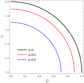
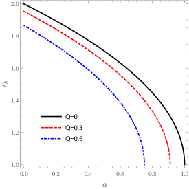
Figure 1: The dependence of the horizon radius $r_{h}$ on the BH charge $Q$ for different values of GB parameter $\alpha$ (left panel) and on the GB coupling constant $\alpha$ for different values of $Q$ (right panel). Note that the horizon behaviour is similar to the one in Einstein gravity in case one of two parameters vanishes.

From Eq. (2.3) there exist two branches of BH solutions. However, we shall restrict ourselves to the minus sign of solution as it exhibits an attractive massive source [178, 179]. We must ensure that this is the right branch, thus we need to expand Eq. (2.3) in small $\alpha$

$$\lim_{\alpha\rightarrow 0}F(r)=1-\frac{2M}{r}+\frac{Q^{2}}{r^{2}}+\frac{(Q^{2}-2Mr)^{2}}{r^{6}}\alpha+...$$ (2.4)

This clearly shows that it exhibits a Reissner-Nordström solution in the case when $\alpha\rightarrow 0$.

Let us then turn to the horizon of $4D$ charged EGB BH. It is given by positive root of $F(r)=0$, and that gives

$$r_{h}=M+\sqrt{M^{2}-Q^{2}-\alpha}\,.$$ (2.5)

As shown from above equation this clearly shows that an extremal BH is given by with horizon $r=M$ in case $\alpha+Q^{2}=M^{2}$ is satisfied. If the term $\alpha+Q^{2}$ dominates over $M^{2}$ the BH then turns into a naked singularity. This issue for $4D$ charged EGB BH was addressed by the authors of [180]. The dependence of BH horizon on $\alpha$ and $Q$ is shown in Fig. 1. As shown in Fig. 1, the GB coupling constant and BH charge exhibit a similar effect that the outer horizon shifts towards to smaller $r$, i.e. to the central singularity. This is in agreement with the fact that the GB coupling constant exhibits a repulsive gravitational effect [14, 34].

3 Particle geodesics around $4D$ charged EGB BH

3.1 massive particle

Here we first study charged particle motion by considering the Hamiltonian of the system [181] around the static and spherically symmetric charged BH spacetime in $4D$ EGB gravity

$$H\equiv\frac{1}{2}g^{\mu\nu}(\pi_{\mu}-qA_{\mu})(\pi_{\nu}-qA_{\nu})\,,$$ (3.1)

where $\pi_{\mu}$ is the canonical four momentum of a charged particle and $A_{\mu}$ is the electromagnetic four-vector potential for $4D$ charged EGB BH and given by

$$A_{\mu}=\left(-\frac{Q}{r},0,0,0\right)\,.$$ (3.2)

Note that we consider the Hamiltonian as a constant, i.e. $H=-m^{2}/2$. For the Hamilton-Jacobi equation, the action $S$ can be then separated in the following form

$$S=\frac{1}{2}m^{2}\lambda-Et+L\varphi+S_{r}(r)+S_{\theta}(\theta)\ ,$$ (3.3)

where $E\equiv-\pi_{t}$ and $L\equiv\pi_{\varphi}$ are the constants of motion and respectively refer to the energy and angular momentum of the charged particle, while $S_{r}$ and $S_{\theta}$ are functions of $r$ and $\theta$. Let us then rewrite the Hamilton-Jacobi equation in the following form

$$-r^{2}\left(F\right)^{-1}\left(-E+\frac{qQ}{r}\right)^{2}+r^{2}F\left(\frac{\partial S_{r}}{\partial r}\right)^{2}+\left(\frac{\partial S_{\theta}}{\partial\theta}\right)^{2}+\frac{1}{\sin^{2}\theta}\left(L-qA_{\varphi}\right)^{2}+m^{2}r^{2}=0\,.$$ (3.4)

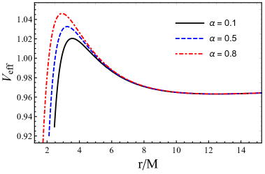
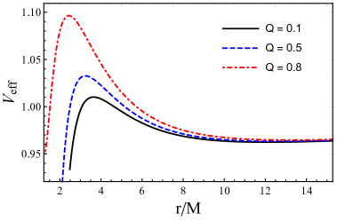
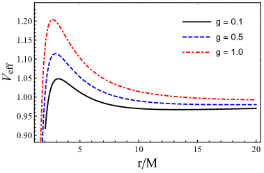
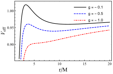
Figure 2: Radial dependence of the effective potential for massive particles orbiting a $4D$ charged EGB BH for $g=0$ on the top and for $g\neq 0$ on the bottom. Top panels: $V_{eff}$ is plotted for different values of $\alpha$ for $Q=0.4$ (left panel) and for different values of $Q$ for $\alpha=0.3$ (right panel). Bottom panels: $V_{eff}$ is plotted for different values of charge parameter $\pm g$ in the case of $\alpha=0.5$ and $Q=0.5$.

	$Q$
$\alpha$	$0.0$	$0.1$	$0.2$	$0.3$	$0.5$	$0.8$
0.0	6.00000	5.98497	5.93957	5.86278	5.60664	4.89077
0.1	5.93782	5.92248	5.87608	5.79755	5.53491	4.79238
0.2	5.87338	5.85768	5.81020	5.72975	5.45987	4.68626
0.3	5.80644	5.79035	5.74167	5.65910	5.38111	4.57055
0.5	5.66395	5.64695	5.59544	5.50782	5.21013	$-$
0.8	5.42276	5.40389	5.34653	5.24829	$-$	$-$

Table 1: The values of $r_{ISCO}$ are tabulated in the case of neutral particle orbiting $4D$ charged EGB BH for various values of GB coupling constant $\alpha$ and BH charge $Q$.

	$g$
$\alpha;Q$	$0.0$	$0.01$	$0.05$	$0.1$	$0.2$	$0.3$
		$-0.01$	$-0.05$	$-0.1$	$-0.2$	$-0.3$
0.1	5.92248	5.92244	5.92230	5.92215	5.92192	3.92179
		5.92251	5.92267	5.92290	5.92341	5.92402
0.2	5.81020	5.81003	5.80936	5.80861	5.80740	5.80659
		5.81038	5.81113	5.81215	5.81443	5.81703
0.3	5.65910	5.65863	5.65684	5.65477	5.65122	5.64853
		5.65958	5.66154	5.66416	5.66987	5.67619
0.5	5.21013	5.20826	5.20091	5.19202	5.17536	5.16044
		5.21201	5.21966	5.22946	5.24983	5.27107

Table 2: The values of $r_{ISCO}$ are tabulated in the case of charged particle orbiting $4D$ charged EGB BH for various values of charge parameter $g$ in the case of fixed $\alpha$ and $Q$. Here we shall for simplicity consider that GB coupling constant and BH charge take the same values, i.e. $\alpha=Q$.

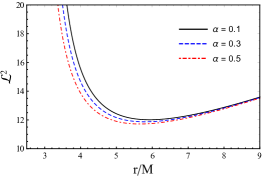
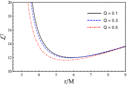
Figure 3: Radial dependence of the angular momentum for charged test particles orbiting around $4D$ charged EGB BH in the case of $g=0.1$. Left panel: $\mathcal{L}^{2}$ is plotted for different values of GB coupling constant $\alpha$ for fixed $Q=0.1$. Right panel: $\mathcal{L}^{2}$ is plotted for different values of BH charge $Q$ for fixed $\alpha=0.1$.

Note that the system can be described by four independent constants of motion of which we have specified three ($E$, $L$, and $m^{2}$). We however restrict ourselves to the equatorial plane ($\theta=\pi/2$) so that we ignore the fourth constant of motion related to the latitudinal motion [181].

From Eq. (3.4), the radial equation of motion for charged particle is written as

$$\dot{r}^{2}=\Big{(}\mathcal{E}-\mathcal{E_{+}}(r)\Big{)}\Big{(}\mathcal{E}-\mathcal{E_{-}}(r)\Big{)}\,,$$ (3.5)

where $\dot{r}^{2}$ must always be positive, and hence we have either $\mathcal{E}>\mathcal{E}_{+}(r)$ or $\mathcal{E}<\mathcal{E}_{-}(r)$. For further analysis, we choose the positive energy $\mathcal{E_{+}}(r)=V_{eff}(r)$ which is physically related to the effective potential. It is then straightforward to define the effective potential for the radial motion of particle in the field of $4D$ charged EGB BH. The effective potential then takes the form

$$V_{eff}(r)=\frac{gQ}{r}+\left(1+\frac{\mathcal{L}^{2}}{r^{2}}\right)^{1/2}\left[1+\frac{r^{2}}{2\alpha}\left(1-\sqrt{1+4\alpha\left(\frac{2M}{r^{3}}-\frac{Q^{2}}{r^{4}}\right)}\right)\right]^{1/2}\,.$$ (3.6)

Here $\mathcal{E}=E/m$ and $\mathcal{L}=L/m$ are the energy and angular momentum per unit mass and $g=q/m$ is the charge parameter per unit mass.

We then analyse the effective potential $V_{eff}(r)$ for the radial motion of both neutral and charged test particles. In Fig. 2, the top panels show the impact of both GB coupling constant $\alpha$ and BH charge $Q$ on the radial profiles of the effective potential for neutral particle, while the bottom panels show the impact of both negative and positive charge parameter $g$ for fixed values of $\alpha$ and $Q$. As seen from radial profile of $V_{eff}(r)$, the height of the effective potential increases with increasing both GB coupling constant $\alpha$ and BH charge $Q$ and the curves shift towards left to smaller $r$. Similarly, we notice that the height of the effective potential also grows for positive charge parameter $g>0$ while with increasing the negative $g<0$ this behaviour turns to opposite in the case of fixed $\alpha$ and $Q$. It is worth noting that the strength of effective potential becomes weaker only for $g<0$ as compered to the one for $g>0$.

Now we turn to the study the circular orbits of charged test particles around $4D$ charged EGB BH characterized by GB coupling term $\alpha$, charge $Q$, and mass $M$. For test particles to be on the circular orbits we need to solve simultaneously

$$V_{eff}(r)=0=V_{eff}^{\prime}(r)\,,$$ (3.7)

where prime refers to a derivative with respect to $r$. The above required conditions give the radii of circular orbits for given values of $\mathcal{L}$. We then determine the angular momentum for charged test particles on the circular orbits

$$\mathcal{L}^{2}=\frac{r^{3}f^{\prime}(r)\Big{(}2f(r)-rf^{\prime}(r)\Big{)}+2Q^{2}g^{2}f(r)}{\Big{(}rf^{\prime}(r)-2f(r)\Big{)}^{2}}+\frac{g\,Q\,f(r)\sqrt{Q^{2}g^{2}+4r^{2}f(r)-2r^{3}f^{\prime}(r)}}{\Big{(}rf^{\prime}(r)-2f(r)\Big{)}^{2}}\,.$$ (3.8)

For neutral test particle, i.e. $g=0$, Eq. (3.8) takes the following form

$$\mathcal{L}^{2}=\frac{r^{3}f^{\prime}(r)}{2f(r)-rf^{\prime}(r)}\,.$$ (3.9)

The radial profiles of the angular momentum of the circular orbits for charged particles are shown in Fig. 3. As shown in Fig. 3 one can easily see that the curves shift towards left to small radii as an increase in the value of both GB coupling constant $\alpha$ and BH charge $Q$ for fixed charge parameter $g$.

Next, let us study the innermost stable circular orbit (ISCO) for both neutral and charged test particles orbiting around $4D$ charged EGB BH. For determining radii of stable circular orbits we should solve the following required condition

$$V_{eff}^{\prime\prime}(r)\geq 0\,.$$ (3.10)

However, for the ISCO radius one needs to solve $V_{eff}^{\prime\prime}(r)=0$. We explore the ISCO radius numerically by solving Eqs. (3.7) and (3.10) simultaneously and provide results in Tables 1 and 2 for both neutral and charged particles. As shown in Table 1 the ISCO radius decreases as both $\alpha$ and $Q$ increase. However, the ISCO radius decreases in the case of negative charge parameter $g<0$ as shown in Table 2.

3.2 massless particle (photon motion)

Here we consider massless particle motion around $4D$ charged EGB BH for which the Hamilton-Jacobi equation is written in the following form

$$H\equiv\frac{1}{2}g^{\mu\nu}\tilde{\pi}_{\mu}\tilde{\pi}_{\nu}=0\,,$$ (3.11)

with $\tilde{\pi}_{\mu}$ and $\tilde{\pi}_{\nu}$ being conserved quantities which are the momentum of massless (photon) particles. It is then sufficient to use Eq. (3.11) to find the effective potential for the photon as follows

$$\tilde{V}_{eff}(r)=\tilde{E}^{2}-F(r)\frac{\tilde{L}^{2}}{r^{2}}\,.$$ (3.12)

where $\tilde{L}$ and $\tilde{E}$ are the conserved quantities, which are the angular momentum and energy of the photon, respectively. To obtain unstable circular orbits for photons we will need to solve following equations

$$\tilde{V}_{eff}(r)=0=\tilde{V^{\prime}}_{eff}(r)\,.$$ (3.13)

In Fig. 4, we show the radius of the photon orbit $r_{ph}$ for various values of $\alpha$ and $Q$ by using Eqs.  (3.12) and (3.13). As expected the photon radius decreases with increasing both GB coupling constant $\alpha$ and BH charge $Q$, see Fig 4.

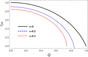
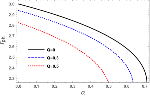
Figure 4: The dependence of the photon radius $r_{ph}$ on the BH charge $Q$ for differnt values of $\alpha$ (left panel) and on the GB coupling constant $\alpha$ for different values of $Q$ (right panel).

4 Weak-field lensing

In this section, we turn to the study optical properties, i.e. weak lensing around $4D$ charged EGB BH. Further we shall for simplicity consider a weak-field case for which Eq. (2.3) can be written as

$$F(r)=1-\frac{R_{g}}{r}+\frac{Q^{2}}{r^{2}}+\frac{\alpha R^{2}_{g}}{r^{4}}\,,$$ (4.1)

with $R_{g}=2M$. For a weak-field approximation we have

$$g_{\alpha\beta}=\eta_{\alpha\beta}+h_{\alpha\beta}\,,$$ (4.2)

where $\eta_{\alpha\beta}$ and $h_{\alpha\beta}$ respectively refer to the expression for Minkowski spacetime and perturbation gravity field describing GR part. Thus, we have [73]

$$\eta_{\alpha\beta} ={\rm diag}(-1,1,1,1)\ ,$$

$$h_{\alpha\beta} \ll 1,\quad h_{\alpha\beta}\rightarrow 0\quad{\rm under}\quad x^{\alpha}\rightarrow\infty\ ,$$

$$g^{\alpha\beta} =\eta^{\alpha\beta}-h^{\alpha\beta},\ \ \ h^{\alpha\beta}=h_{\alpha\beta}\ .$$ (4.3)

Following [73], we consider the weak-field approximation and plasma medium for the light propagation along $z$ axis [73, 76] to get the gravitational deflection equation as

$$\hat{\alpha}_{i} =\frac{1}{2}\int_{-\infty}^{\infty}\bigg{(}h_{33_{,}i}+\frac{\omega^{2}}{\omega^{2}-\omega^{2}_{e}}h_{00_{,}i}-\frac{K_{e}}{\omega^{2}-\omega^{2}_{e}}N{{}_{,}i}\bigg{)}dz.$$ (4.4)

Here, $\hat{\alpha}_{i}$ would be negative and positive respectively for the deflection of the light trajectory, depending on the light moving either towards or away from the central object. In the above equation, $\omega_{e}$ can be set $\omega(\infty)=\omega$ at infinity as limitations. For the weak field approach, the BH spacetime metric can be written in the following form [76]

$$ds^{2}=ds^{2}_{0}+\left(\frac{R_{g}}{r}-\frac{Q^{2}}{r^{2}}-\frac{\alpha R^{2}_{g}}{r^{4}}\right)dt^{2}+\left(\frac{R_{g}}{r}-\frac{Q^{2}}{r^{2}}-\frac{\alpha R^{2}_{g}}{r^{4}}\right)dr^{2}\,,$$ (4.5)

with $ds^{2}_{0}=-dt^{2}+dr^{2}+r^{2}(d\theta^{2}+\sin^{2}\theta d\phi^{2})$ corresponding to Minkowski metric. Further, $h_{\alpha\beta}$ can be written in the Cartesian coordinates system as follows

$$h_{00}= \left(\frac{R_{g}}{r}-\frac{Q^{2}}{r^{2}}-\frac{\alpha R^{2}_{s}}{r^{4}}\right),$$

$$h_{ik}= \left(\frac{R_{g}}{r}-\frac{Q^{2}}{r^{2}}-\frac{\alpha R^{2}_{s}}{r^{4}}\right)n_{i}n_{k}\ ,$$

$$h_{33}= \left(\frac{R_{g}}{r}-\frac{Q^{2}}{r^{2}}-\frac{\alpha R^{2}_{s}}{r^{4}}\right)\cos^{2}x\;,$$ (4.6)

with $\cos x=z/\sqrt{b^{2}+z^{2}}$ and $r=\sqrt{b^{2}+z^{2}}$ [76].

Introducing new notation as $h_{\alpha\beta}$ in Eq. (4.6) one can rewrite the expression of the gravitational deflection angle in terms of the impact parameter $b$ for $4D$ charged EGB BH immersed in plasma medium. Thus, we have

$$\hat{\alpha}_{b}=\int_{-\infty}^{\infty}\frac{b}{2r}\Bigg{(}\partial_{r}\bigg{(}\bigg{(}\frac{R_{g}}{r}-\frac{Q^{2}}{r^{2}}-\frac{\alpha R^{2}_{s}}{r^{4}}\bigg{)}\cos^{2}x\bigg{)}+\partial_{r}\bigg{(}\frac{R_{g}}{r}-\frac{Q^{2}}{r^{2}}-\frac{\alpha R^{2}_{s}}{r^{4}}\bigg{)}\frac{\omega^{2}}{\omega^{2}-\omega^{2}_{e}}-\frac{K_{e}}{\omega^{2}-\omega^{2}_{e}}\partial_{r}N\Bigg{)}dz\,.$$ (4.7)

Next, we will analyze the deflection angle for homogeneous and inhomogeneous cases in detail.

4.1 Uniform plasma

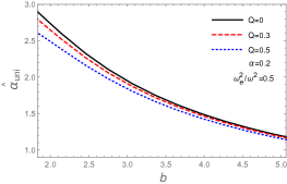
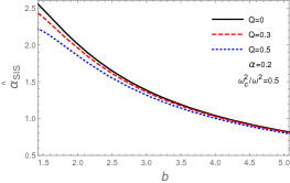
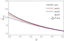
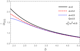
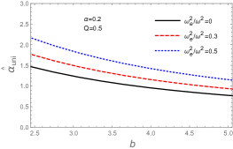
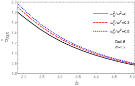
Figure 5: Left column: shows the variation of deflection angle $\hat{\alpha}_{b}$ as a function of the impact parameter $b$ in uniform plasma for different combinations of BH charge $Q$, GB coupling constant $\alpha$ and plasma parameter $\frac{\omega^{2}_{e}}{\omega^{2}}$. Right column: shows the variation of deflection angle $\hat{\alpha}_{b}$ for the case corresponding cases in presence of non-uniform plasma.

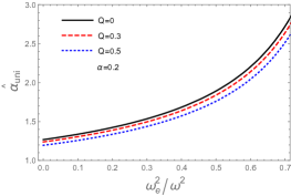
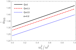
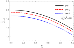
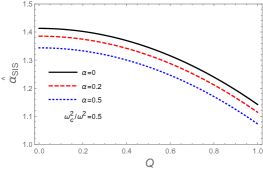
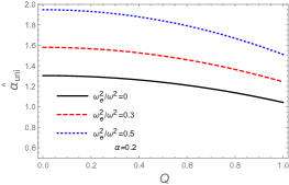
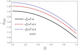
Figure 6: Left column: shows the variation of deflection angle $\hat{\alpha}_{b}$ in the presence of uniform-plasma as a function of plasma parameter (top panel) and charge $Q$ (middle and bottom panels) for different combinations of GB coupling constant $\alpha$. Similarly, right column: shows the variation of deflection angle $\hat{\alpha}_{b}$ for the corresponding cases in the presence of non-uniform plasma. Here, for both the columns $b=3$.

We now analyse the light deflection with a uniform plasma medium. From Eq. (4.7), one can easily obtain the following new expression

$$\hat{\alpha}_{\mathrm{uni}}=-\bigg{(}\frac{\omega^{2}}{\omega^{2}-\omega^{2}_{e}}\bigg{)}\bigg{(}\frac{\pi Q^{2}}{2b^{2}}-\frac{R_{g}}{b}+\frac{3\pi\alpha R^{2}_{s}}{4b^{4}}\bigg{)}-\bigg{(}\frac{\pi Q^{2}}{4b^{2}}-\frac{R_{g}}{b}+\frac{3\pi\alpha R^{2}_{s}}{16b^{4}}\bigg{)}\,.$$ (4.8)

For the uniform plasma $\partial_{r}N=0$ is always satisfied. We now provide plots representing the behaviour of deflection angle for various parameters such as the GB coupling constant $\alpha$, BH charge $Q$, and the plasma medium parameter $\frac{\omega^{2}_{e}}{\omega^{2}}$. Note that here we use Eq. (4.8) to show the above mentioned plots in Figs. 5 and 6. As could be seen from Figs. 5 and 6 the deflection angle decreases with increasing the values of $\alpha$ and $Q$, while this behaviour is opposite with increasing the value of plasma medium parameter $\frac{\omega^{2}_{e}}{\omega^{2}}$. Thus, the circular orbits of light propagation can become close to the central object due to the impact of the GB coupling constant and BH charge, as shown in Figs. 5 and 6. However, the deflection angle increases as that of the plasma medium parameter $\frac{\omega^{2}_{e}}{\omega^{2}}$ regardless of $\alpha$ and $Q$, which are regarded as gravitational repulsive charges. From an observational point of view, far away observer could observe an image larger than the object due to the plasma effect.

4.2 Non-uniform plasma

Here we consider the gravitational deflection angle by the $4D$ charged EGB BH in presence of a singular isothermal sphere (SIS) plasma medium which would play an important role in studying lensing properties of galaxies and clusters [73].

Following [73, 76] the distribution of density and the plasma concentration will respectively read as follows:

$$\rho(r)=\frac{\sigma^{2}_{v}}{2\pi r^{2}},$$ (4.9)

with $\sigma^{2}_{v}$ being a 1D velocity dispersion and

$$N(r)=\frac{\rho(r)}{\kappa m_{p}}\,,$$ (4.10)

with mass of proton $m_{p}$ and a 1D coefficient $\kappa$ related to the dark matter contribution.

From Eq. (4.7) the gravitational deflection angle for the non-uniform plasma medium can be obtained as [73],

$$\hat{\alpha}_{\mathrm{SIS}}=\frac{\omega^{2}_{c}R^{2}_{g}}{\omega^{2}b^{2}}\bigg{(}\frac{1}{2}-\frac{3Q^{2}}{8b^{2}}-\frac{2R{{}_{g}}}{3b\pi}+\frac{5\pi\alpha R^{2}_{s}}{8b^{4}}\bigg{)}-\bigg{(}\frac{3\pi Q^{2}}{4b^{2}}-\frac{2R_{g}}{b}+\frac{15\pi\alpha R^{2}_{s}}{16b^{4}}\bigg{)}\,,$$ (4.11)

where $\omega^{2}_{c}$ represents another plasma constant, and that is introduced as [76, 81]

$$\omega^{2}_{c}=\frac{\sigma^{2}_{v}K_{e}}{2\kappa m_{p}R^{2}_{g}}\,.$$ (4.12)

Using Eq. (4.12), we provide plots which reflect the role of non-uniform plasma, the GB coupling constant and BH charge for the gravitational lensing properties. The dependence of the deflection angle on impact parameter of orbits $b$ is shown in the right column of Fig. 5. For large values of the impact parameter $b$ the deflection angle approaches to the zero in the case when $Q$ and $\alpha$ and $\frac{\omega^{2}_{e}}{\omega^{2}}$ are taken into account, see right column of Fig. 5. The deflection angle as a function of BH charge $Q$ and plasma parameter $\frac{\omega^{2}_{e}}{\omega^{2}}$ is shown in right column of Fig. 6. The top panel in the right column of Fig. 6, reflects the deflection angle as a function of plasma parameter $\frac{\omega^{2}_{e}}{\omega^{2}}$ for different values of $Q$ for fixed $\alpha$, while the middle and bottom panels respectively reflect the deflection angle as a function of BH charge $Q$ for different values of $\alpha$ for fixed $\frac{\omega^{2}_{e}}{\omega^{2}}$ and for vise versa. From right column of Figs. 5 and 6 one can easily notice that the GB coupling constant and BH charge have similar effect that decreases the deflection angle. However, the deflection angle increases linearly in the presence of non-uniform plasma medium surrounding BH in comparison to uniform-plasma where it increases exponentially (see top row of Fig. 6). It is worth noting here that the deflection angle in the presence of non-uniform plasma is smaller than in the presence of uniform plasma medium.

5 Collision and Centre-of-mass energy

5.1 Centre-of-mass energy of two colliding spinless charged particles

We now study the particle acceleration process of two charged particles colliding near the horizon of the $4D$ charged EGB BH. We shall consider two particles that have rest masses $m_{1}$ and $m_{2}$ at a distance far away from BH for simplicity. Let us write the four-momentum and the total momenta for colliding two particles $(i=1,2)$ as

$$p_{i}^{\alpha} = m_{i}u_{i}^{\alpha},$$

$$p_{t}^{\alpha} = p_{1}^{\alpha}+p_{2}^{\alpha}\,.$$ (5.1)

with the four velocity $u_{i}^{\mu}$ of particle $i$ and the four-momentum $\pi^{\alpha}$ which is given by

$$\pi^{\alpha}=g^{\mu\nu}\left(\pi_{\nu}-qA_{\nu}\right)\,.$$ (5.2)

Following to [115] and Eq. (5.1) the extracted energy $E_{C.M.}$ by collision between two particles is defined by

$$\frac{E_{C.M.}^{2}}{2m_{1}m_{2}}=\frac{m_{1}^{2}+m_{2}^{2}}{2m_{1}m_{2}}-g_{\alpha\beta}u^{\alpha}_{1}u^{\beta}_{2}\,.$$ (5.3)

The above the center of mass energy $E_{C.M.}$ allows to understand how the GB coupling constant $\alpha$ and BH charge $Q$ impact on the extracted energy by collision of two particles. In this respect, it would be important to study the extracted energy in the $4D$ charged BH in EGB gravity and compare to Einstein gravity. In other words this collision mechanism could play a crucial role in explaining high energy particle processes in the vicinity of BH candidates. Further for simplicity we assume two free falling particles collide at the near horizon. In doing so, using Eqs. (5.1) and (5.3) we obtain

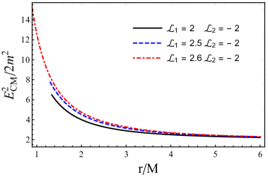
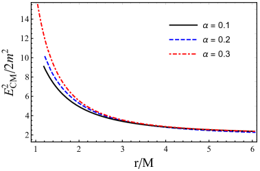
Figure 7: The behaviour of $E_{C.M}$ vs $r$ for two non-spinning particles colliding near the horizon of a 4D charged EGB BH is presented. For the left panel, we select the extreme BH case (i.e. $r_{h}/M=1$) and set the values of the parameters $\alpha$ and $Q$ appropriately for various combinations of $\mathcal{L}_{1}$ and $\mathcal{L}_{2}$. For the right panel, the parameters $Q$, $\mathcal{L}_{1}$, and $\mathcal{L}_{2}$ are set to $0.8$, $2.6$, and $-2$, respectively, and the parameter $\alpha$ is varied in 0.1-step increments from 0.1 to 0.3. Here, the value energy for both particles is set to unity.

$$\frac{E^{2}_{C.M.}}{2m_{1}m_{2}} =1+\frac{\left(m_{1}-m_{2}\right)^{2}}{2m_{1}m_{2}}+\frac{\tilde{\mathcal{E}}_{1}\tilde{\mathcal{E}}_{2}}{F(r)}-\frac{\mathcal{L}_{1}\mathcal{L}_{2}}{r^{2}}-\frac{\sqrt{\tilde{\mathcal{E}}_{1}^{2}-F(r)\left(1+\frac{\mathcal{L}_{1}^{2}}{r^{2}}\right)}\sqrt{\tilde{\mathcal{E}}_{2}^{2}-F(r)\left(1+\frac{\mathcal{L}_{2}^{2}}{r^{2}}\right)}}{F(r)}\,,$$ (5.4)

where we have defined $\tilde{\mathcal{E}}_{i}=\mathcal{E}_{i}-q_{i}Q/r$ and we have set $M=1$. The extracted energy is given by Eq. (5.4) for the collision of two particles with energies $\mathcal{E}_{1,2}$ and specific angular momenta $\mathcal{L}_{1,2}$. Let us then evaluate the center-of-mass energy extracted by the freely falling charged particles colliding near the BH horizon. For evaluating $E_{C.M.}$ we shall for simplicity assume free falling particles $m_{1,2}=m$ and these two particles have different angular momenta $\mathcal{L}_{1}=\mathcal{L}_{max}$ and $\mathcal{L}_{2}=\mathcal{L}_{min}$ (where $\mathcal{L}_{min}$ and $\mathcal{L}_{max}$ are angular momenta of the two charged particles falling into the black hole with opposite directions). In Fig. 7, we show the radial dependence of $E_{C.M.}$ energy. As can bee seen from Fig. 7 the minimum energy occurs when two charged particles have opposite angular momentum. However, the extracted energy goes up with increasing $\mathcal{L}_{1}=\mathcal{L}_{max}$. We note that $E_{C.M.}$ reaches its maximum value as a consequence of the increase in value for the coupling constant $\alpha$ for fixed value of $Q$, thus resulting in increasing the value for the extracted energy in contrast to the RN BH.

We now consider the limiting case $r\to r_{h}$ so as to find the highest values of the center of mass energy. Considering $E_{1}/m_{1}=E_{2}/m_{2}=1$ for free falling particles we then have the limiting value of $E_{C.M.}$ at the horizon

$$\frac{E^{2}_{C.M.}(r\rightarrow r_{h})}{m^{2}}\approx\Big{[}4+\left(1-6\sqrt{1-Q^{2}-\alpha}\right)\Big{(}\mathcal{L}_{1}-\mathcal{L}_{2}\Big{)}^{2}\Big{]}\,.$$ (5.5)

As seen from Eq. (5.5) this clearly shows that the limiting value of center of mass energy extracted by collision of two particles at the horizon increases due to the impact of the GB coupling constant and BH charge. That is, the horizon radius can become arbitrarily close to the BH as the coupling constant and BH charge increase.

5.2 Centre-of-mass energy in the context of spinning massive test particles

It is shown that centre of mass energy ($E_{C.M.}$) for two colliding equal-mass non-(spinning [160]) [182] particles becomes maximum. However, the maximum $E_{C.M.}$ for non-spinning particles case has an upper bound [115] while there is no upper bound if the colliding particles are spinning [155, 157]. For rotating BHs, the maximum $E_{C.M.}$ increases in comparison with their non-rotating counterparts and becomes infinite when the rotating BH satisfies an extremal condition. In this subsection, our main goal is to bring out the effect of particle’s spin on the $E_{C.M.}$.

The $E_{C.M.}$ of two colliding equal mass spinning test particles falling from rest at infinity is defined as

$$E_{C.M.}^{2} \equiv-(P_{1\mu}+P_{2\mu})(P_{1}^{\mu}+P_{2}^{\mu}),$$

$$=-\left(P_{1\mu}P_{1}^{\mu}+P_{2\mu}P_{2}^{\mu}+P_{1\mu}P_{2}^{\mu}+P_{2\mu}P_{1}^{\mu}\right),$$

$$=-2\left(-m^{2}+P_{1\mu}P_{2}^{\mu}\right)=2m^{2}\left(1-\frac{P_{1\mu}P_{2}^{\mu}}{m^{2}}\right).$$ (5.6)

Now, by using Eqs. (B.1), (B.2) and (B.3) in the above Eq. (5.6), the $E_{C.M.}$ per unit mass reads as

$$\left(\frac{E_{C.M.}}{m}\right)^{2} =2\left[1+\left(1+\frac{\left(r^{2}-\mathcal{B}\right)}{2\alpha}\right)^{-1}\mathcal{K}_{1}\mathcal{K}_{2}-\frac{1}{r^{2}}\mathcal{Z}_{1}\mathcal{Z}_{2}-\left(1+\frac{\left(r^{2}-\mathcal{B}\right)}{2\alpha}\right)^{-1}\right.$$

$$\left.\times\sqrt{\mathcal{K}_{1}^{2}-\left(1+\frac{\left(r^{2}-\mathcal{B}\right)}{2\alpha}\right)\left[1+\frac{\mathcal{Z}_{1}^{2}}{r^{2}}\right]}\,.\sqrt{\mathcal{K}_{2}^{2}-\left(1+\frac{\left(r^{2}-\mathcal{B}\right)}{2\alpha}\right)\left[1+\frac{\mathcal{Z}_{2}^{2}}{r^{2}}\right]}\right]$$ (5.7)

From straightforward calculations, the above equation yields

$$\left(\frac{E_{C.M.}}{m}\right)^{2} =\frac{2}{\Delta\Pi_{1}\Pi_{2}}\Bigg{[}\left(2\alpha r\mathcal{B}E_{1}-\tilde{S}_{1}J_{1}\mathcal{C}\right)\left(2\alpha r\mathcal{B}E_{2}-\tilde{S}_{2}J_{2}\mathcal{C}\right)+\Delta\Big{[}\Pi_{1}\Pi_{2}-4\alpha^{2}\mathcal{B}^{2}$$

$$\times\left(J_{1}-E_{1}S_{1}\right)\left(J_{2}-E_{2}S_{2}\right)\Big{]}-\sqrt{\left(2\alpha r\mathcal{B}E_{1}-\tilde{S}_{1}J_{1}\mathcal{C}\right)^{2}-\Delta\Big{[}\Pi_{1}^{2}+4\alpha^{2}\mathcal{B}^{2}\left(J_{1}-E_{1}S_{1}\right)^{2}\Big{]}}$$

$$\times\sqrt{\left(2\alpha r\mathcal{B}E_{2}-\tilde{S}_{2}J_{2}\mathcal{C}\right)^{2}-\Delta\Big{[}\Pi_{2}^{2}+4\alpha^{2}\mathcal{B}^{2}\left(J_{2}-E_{2}S_{2}\right)^{2}\Big{]}}\Bigg{]},$$ (5.8)

where $\Delta\equiv F(r)\equiv\left[1+(1/2\alpha)\left(r^{2}-\mathcal{B}\right)\right]$, $\mathcal{C}\equiv 2\alpha r\mathcal{AB}$ and $\Pi_{1,2}\equiv(2\alpha r\mathcal{B}-\tilde{S}_{1,2}^{2}\mathcal{C})$. From Eq. (5.8), one can easily deduce that $E_{C.M.}$ could possibly become infinitely high not only at horizon of $4D$ charged EGB BH $\Delta=0$, but also at either $\Pi_{1}=0$ or $\Pi_{2}=0$. However, for the former case, it is already a well established fact that a static spherically symmetric BH $E_{C.M.}$ will not diverge at the horizon. Also, for the later case, the potential divergence of $E_{C.M.}$ will occurs at some radial distance, but this is not straightforward in nature due to the same reason, as mentioned in [155] for Schwarzschild BH. In the present subsection, we will consider another interesting scenario where the collision occurs near the horizon but outside it (i.e., $r_{0}<r_{h}=M+\sqrt{M^{2}-Q^{2}-a}$). Therefore, the only way to diverge for $E_{C.M.}$ extracted by the collision of two spinning particles is to make $\Delta$ small enough.

5.2.1 Classification of spinning particle and their different combinations

Now, in order to discuss this case in more detail, we need to classify the spinning particle into three types, i.e. usual particle, critical particle and near-critical particle, as mentioned in [157]. A particle is known as usual if:

$$\mathcal{K}_{h}\equiv\frac{E-\tilde{S}J\mathcal{A}_{h}}{1-\tilde{S}^{2}A_{h}}\neq 0\,.$$ (5.9)

Here and hereafter “$h$" in the subscript means that the value of corresponding quantity is taken at the horizon $r_{h}$. On the other hand, a particle is considered as critical if $\mathcal{K}_{h}=0$ always

$$E-\tilde{S}J\mathcal{A}_{h}=0\,.$$ (5.10)

Then, $\mathcal{K}$ near the horizon reads as

$$\mathcal{K}\approx\left[\frac{J\tilde{S}\left(3Mr_{h}\left(r_{h}^{3}-4\alpha M\right)-4Q^{2}\left(r_{h}^{3}-\alpha M\right)\right)}{r_{h}^{2}\left(8\alpha Mr_{h}-4\alpha Q^{2}+r_{h}^{4}\right)^{3/2}\left(1-\tilde{S}^{2}A_{h}\right)}\right](r-r_{h})\,.$$ (5.11)

Thus, at the colliding radius $r=r_{c}$ where $\mathcal{K}_{c}=O(\Delta_{c})$, the second term dominates Eq. (B.3) so that $(P^{r}/m)_{c}$ becomes imaginary, and hence such a spinning particle cannot reach the $r_{h}$ of $4D$ charged EGB BH (hereafter “$c$" in the subscript means that the value of corresponding quantity is taken at the point of collision $r_{c}$). And, a colliding spinning particle is known as near-critical particle if and only if $\mathcal{K}_{h}=\sqrt{r_{c}-r_{h}}$ is satisfied

$$E-\tilde{S}J\mathcal{A}_{h}=O\left(\sqrt{r_{c}-r_{h}}\right)\,.$$ (5.12)

Let us then consider different combinations of colliding particles depending upon the classification done till now and check, for which combination of two colliding spinning particles the divergence of $E_{C.M.}$ can occur as follows:

• Case I: When both colliding spinning particles are usual (i.e. $P_{1}=P_{2}=usual$) it is easy to check from Eq. (5.8) that $E_{C.M.}$ is finite and hence the BSW effect is absent. The same has already been stated earlier in this section that if the collision of two spinning particles will take place at the $r_{h}$, $E_{C.M.}$ then becomes finite.

• Case II: When one of the two colliding particles is critical and the other one is usual (i.e. $P_{1}=critical$ and $P_{2}=usual$), then $P_{1}$ cannot reach the horizon. Hence, no collision will take place near $r_{h}$ and $E_{C.M.}$ becomes finite, thereby indicating that the BSW effect is absent.

• Case III: When both the particles are critical (i.e. $P_{1}=P_{2}=critical$), then again both the particles cannot reach the horizon. Hence no collision take place near $r_{h}$, and thus the BSW effect is absent.

• Case IV: In the case in which particle $P_{1}$ is $near-critical$ and particle $P_{2}$ is $usual$: let us suppose that for $P_{1}$

  $$\mathcal{K}_{h}=\mathcal{C}\sqrt{\Delta_{c}}+O(\Delta_{c}),$$ (5.13)

  where $\mathcal{C}$ is some finite nonvanishing coefficient corresponding to $P_{1}$. Let us now consider that at the point of collision $\mathcal{K}_{c}\approx\mathcal{K}_{h}+O(\Delta_{c})$ and therefore the second part of Eq. (5.6) (i.e. $-P_{1\mu}P_{2}^{\mu}/m^{2}$) becomes

  $$-\frac{P_{1\mu}P_{2}^{\mu}}{m^{2}} \approx\frac{1}{m^{2}}\left(\frac{P_{1c}^{t}P_{2h}^{t}-P_{1c}^{r}P_{2h}^{r}}{\Delta_{c}}\right)$$

  $$=\frac{\mathcal{K}_{2h}}{\Delta_{c}}\left[\mathcal{K}_{1c}-\left(\sqrt{\mathcal{K}^{2}-\Delta\left(1+\frac{\mathcal{Z}^{2}}{r^{2}}\right)}\right)_{1c}\right],$$ (5.14)

  where $\mathcal{Z}=(J-E\tilde{S})/(1-\tilde{S}^{2}\mathcal{A})$. It is worth to mention here that in Eq. (5.14), we neglect the expression for ($P_{1r}P_{2}^{r}$) as it remains finite and does not contribute to $E_{C.M.}$ to let it diverge. Using Eqs. (5.10) and (5.13), Eq. (5.14) takes the form

  $$-\frac{P_{1\mu}P_{2}^{\mu}}{m^{2}} \approx\frac{\mathcal{K}_{2h}}{\sqrt{\Delta_{c}}}\left[\mathcal{C}_{1}-\left(\sqrt{\mathcal{C}^{2}-1-\frac{E^{2}}{r_{h}^{2}\tilde{S}^{2}\mathcal{A}_{h}^{2}}}\right)_{1}\right]\,.$$ (5.15)

  It is easy to check that Eq. (5.15) diverges in the limit when $\Delta_{c}\to 0$. Therefore, we have successfully found the case where $E_{C.M.}$ will grow illimitably. Further, in the limit when $\alpha\to 0$ and $Q=0$, the expression for $A_{h}$ reduces to $M/r_{h}^{3}$ and Eq. (5.15) takes the form

  $$-\frac{P_{1\mu}P_{2}^{\mu}}{m^{2}} \approx\frac{\mathcal{K}_{2h}}{\sqrt{\Delta_{c}}}\left[\mathcal{C}_{1}-\left(\sqrt{\mathcal{C}^{2}-1-\frac{16M^{2}E^{2}}{\tilde{S}^{2}}}\right)_{1}\right]\,,$$ (5.16)

  which is the same as found in [157] for Schwarzschild BH case.

• Case V: When particle $P_{1}$ is near-critical and particle $P_{2}$ is critical, then again $P_{2}$ cannot reach the horizon. Hence, no collision will take place near the horizon and $E_{C.M.}$ will not grow infinitely.

• Case VI: When both $P_{1}$ and $P_{2}$ are near-critical particles, $-P_{1\mu}P_{2}^{\mu}/m^{2}$ comes out as

  $$-\frac{P_{1\mu}P_{2}^{\mu}}{m^{2}} \approx 1+\frac{E^{2}}{\left(r_{h}\tilde{S}\mathcal{A}_{h}\right)^{2}}\,,$$ (5.17)

  which is a finite quantity. Hence, $E_{C.M.}$ is finite and thus again BSW effect is absent.

It is important to note here that out of all six possible cases of two spinning particles only for the case IV (i.e. combination of near-critical and usual particles) unbound growth of $E_{C.M.}$ is obtained if and only if the term under square root in (5.15) is positive. Thus, any $near-critical$ particle having the same mass as usual particle and satisfying the following condition:

$$\mathcal{C}^{2} >1+\frac{E^{2}}{r_{h}^{2}\tilde{S}^{2}\mathcal{A}_{h}^{2}}\,,$$ (5.18)

which is required for obtaining the unbounded $E_{C.M.}$

5.2.2 Bypassing the superluminal motion of spinning particle

For spinning particles it is a well known fact that the four-velocity $u^{\mu}$ is not a conserved quantity and hence their motion can be timelike (subluminal) and spacelike (superluminal). Using the relation between $u^{\mu}$ and four-momentum $P^{\mu}$ from Eqs. (B.9) and (B.10), the ratio of the square of the four velocity ($u_{\mu}u^{\mu}$) to the square of time component $\left(u^{t}\right)^{2}$ of $u^{\mu}$ reads as

$$U^{2}\equiv\frac{u_{\mu}u^{\mu}}{\left(u^{t}\right)^{2}} =-\Delta^{2}\left(\frac{1-\tilde{S}^{2}\mathcal{A}}{E-\tilde{S}J\mathcal{A}}\right)^{2}\left(1-\Psi\right)\,,$$ (5.19)

where

$$\Psi =\tilde{S}^{2}\left(\frac{J-E\tilde{S}}{r\left(1-\tilde{S}^{2}\mathcal{A}\right)^{2}}\right)^{2}\left[\mathcal{A}\left(2-\tilde{S}^{2}\mathcal{A}\right)+\Delta^{\prime\prime}\left(1-\frac{\tilde{S}^{2}\Delta^{\prime\prime}}{4}\right)\right]$$ (5.20)

Here, “$\;{}^{\prime}\;$” denotes the derivative with respect to radial coordinate $r$. The variation of parameter space between $r$ and $\tilde{S}$ where $U^{2}$ is subluminal (i.e., less than zero) is shown in Fig. 8 for different combinations of $Q,\alpha,E$ and $J$. As was mentioned previously 5.2 there appears a potential divergence of $E_{C.M.}$ (via Eq. (5.8)) near the point $\Pi(r_{0})=0\Rightarrow 1-\tilde{S}^{2}\mathcal{A}=0$ which leads to the problems such as superluminal motion and causality, as Eq. (5.19) changes its sign from negative to positive at this location $r_{0}$. However, we have shown in previous subsection 5.2.1 that if we consider the collision of near-critical and usual particles near the horizon but outside it, then also there is a possiblity of unbounded $E_{C.M.}$. Hence, we are only interested in the region $r>r_{h}$ and want to have square of the four velocity less than zero in this region in order to bypass the superluminal motion of spinning particles. This necessity of bypassing of superlumial region leads $\Psi<1$. Taking into account the condition $\mathcal{K}\geq 0$, from Eq. (5.9) we have:

$$\varkappa\equiv\tilde{S}^{2}\mathcal{A}_{h}<1\,,$$ (5.21)

and from Eq. (5.20), one can infer that $\Psi$ is a monotonically decreasing function of $r$. Therefore, it is ample to show that

$$\Psi(r_{h})<1\,,$$ (5.22)

because for any radial distance $r>r_{h}$, one will have $\Psi(r)<\Psi(r_{h})<1$. As was shown in the previous subsection that unbound $E_{C.M.}$ is possible only for the case IV (i.e. $P_{1}=$near-critical and $P_{2}=$usual). Therefore, as far as particle $p_{2}$ is concerned, it is enough to take a $\tilde{S}=0$ particle. This condition leads to $\Psi=0$ and hence condition (5.22) is satisfied automatically. Also, for $\tilde{S}\neq 0$ but finite, the condition (5.22) holds well because one can easily choose $\left|J-E\tilde{S}\right|$ small enough as $J$ and $E$ are independent quantities. Hence, we assume that for usual particle the condition (5.22) holds well.

Now for the near-critical particle, the conserved energy $E$ and the total angular momentum $J$ are related via Eq. (5.10). Using Eqs. (5.10), (5.20) and (5.21), we obtain the condition

$$E<\frac{\mathcal{A}_{h}r_{h}(1-\varkappa)}{\sqrt{\mathcal{A}_{h}(2-\varkappa)+\Delta^{\prime\prime}_{h}\left(1-\frac{\tilde{S}^{2}\Delta^{\prime\prime}_{h}}{4}\right)}}\,.$$ (5.23)

Inequality (5.23) is multi-variable in nature and hence it is difficult to analyse it analytically. Therefore, we numerically find the region (see Fig. 9) where this inequality is satisfied. From Fig. 9, it is easy to conclude that as the parameter $Q$ increases the allowed (shaded) region for $E$ increases. However, this increment is small for smaller values of GB coupling constant $\alpha$. Similarly, the allowed region increases as we increase the parameter $\alpha$, keeping parameter $Q$ constant. On contrary to $Q$ and $\alpha$, the allowed region decreases as parameter $\tilde{S}$ increases.

Using Eq. (5.10) in condition (5.23), the inequality in $J$ becomes

$$J<\frac{\tilde{S}\mathcal{A}_{h}r_{h}(1-\varkappa)}{\varkappa\sqrt{\mathcal{A}_{h}(2-\varkappa)+\Delta^{\prime\prime}_{h}\left(1-\frac{\tilde{S}^{2}\Delta^{\prime\prime}_{h}}{4}\right)}}$$ (5.24)

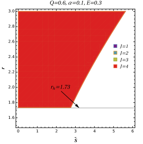
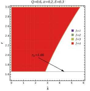
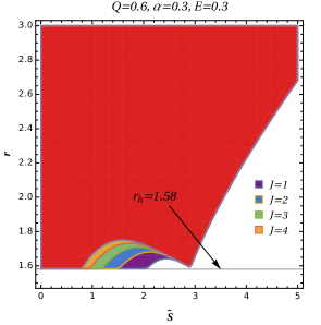
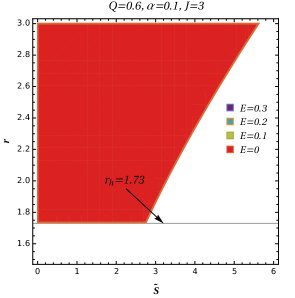
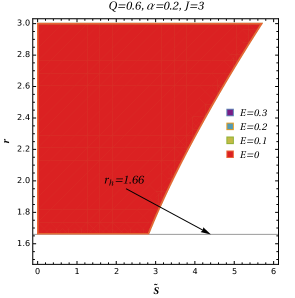
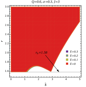
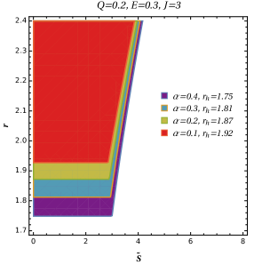
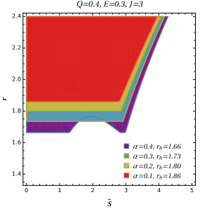
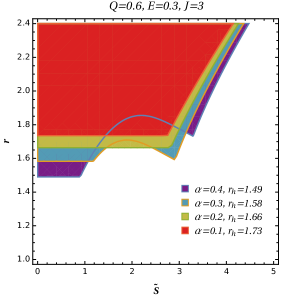
Figure 8: Plots show the allowed region between spin parameter $\tilde{S}$ and $r$ for which $U^{2}$ is subluminal (i.e. less than zero). In first row: variation of parameter space between $\tilde{S}$ and $r$ for different values of $J$ is shown. Here, $Q$ and $E$ are fixed to $0.6$ and $0.3$, respectively while parameter $\alpha$ varies from 0.1 (left) to 0.3 (right). In second row: variation of parameter space between $\tilde{S}$ and $r$ for different values of $E$ is shown. Here, $Q$ and $J$ are fixed to $0.6$ and $3$, respectively while parameter $\alpha$ again varies from 0.1 (left) to 0.3 (right). In third row: variation of parameter space between $\tilde{S}$ and $r$ for different values of $\alpha$ is shown. Here, $E$ and $J$ are fixed to $0.3$ and $3$, respectively while parameter $Q$ varies from 0.2 (left) to 0.6 (right). Here, mass parameter of $4D$ EGB BH set to unity.

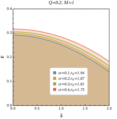
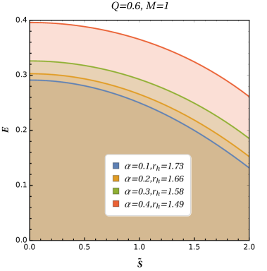
Figure 9: Plots show the variation of allowed (shaded) region for $E$ as parameter $\tilde{S}$ increases for different combinations of $Q$ and $\alpha$.

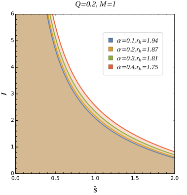
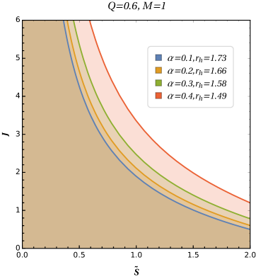
Figure 10: Plots show the variation of allowed (shaded) region for $J$ as parameter $\tilde{S}$ increases for different combinations of $Q$ and $\alpha$.

In Fig. 10, we show the variation of total angular momentum $J$ as a function of particle spin $\tilde{S}$ for different combinations of $Q$ and $\alpha$, using the inequality relation (5.24). From Fig. 10 one can observe that as the parameter $Q$ increases the allowed (shaded) region for $J$ increases only for the fixed $\alpha\geq 0.3$. However, there is no visible increment for smaller values $\alpha$. Additionally, the allowed region increases as we increase the parameter $\alpha$ for the fixed $Q$. In contrary to $Q$ and $\alpha$, the allowed region decreases as parameter $\tilde{S}$ increases. It is interesting to note from Fig. 10 that for smaller values of $\tilde{S}$ there exists no bound on the value of $J$.

Using Eq. (5.10) in Eq. (B.2) for near critical particle, we have

$$\left(\frac{J-E\tilde{S}}{1-\tilde{S}^{2}\mathcal{A}}\right)\approx J=\frac{E}{\tilde{S}\mathcal{A}_{h}}>0\,,$$ (5.25)

which indicates that only prograde orbits can lead to infinitely high $E_{C.M.}$ values.

From condition (5.23) and Fig. 10, we conclude that if a near-critical particle is coming from infinity (i.e., $E\geq 1$) then infinitely high $E_{C.M.}$ cannot be observed until and unless a multiple scattering scenario is achieved rather than the direct collision. This infers that a particle coming from rest at infinity collides near the horizon of BH and achieves the bounding values to satisfy the near-critical conditions for infinitely $E_{C.M.}$ to be produced in the next collision. However, infinitely high $E_{C.M.}$ could possibly be observed if and only if the particle is regarded as a near-critical particle which starts from a distance $r>r_{h}$, where condition (5.23) is always satisfied.

6 Conclusions and discussions

In the this paper, we have carried out the calculations for the weak gravitational lensing in the context of both uniform and non-uniform plasma, whereas the BSW mechanism (i.e. BH as a particle accelerator) is studied for non-spinning and spinning particles around the charged $4D$ EGB BH spacetime, and examined the effect of Gauss-Bonnet coupling paramter $\alpha$ and charge parameter $Q$ on these phenomena. We also compared the results with those of RN (i.e., $\alpha\rightarrow 0$) and $4D$ EGB BHs (i.e., $Q\rightarrow 0$). Although the measurement of weak gravitational lensing effects with enough accuracy are improbable at present but in near future with the advancement of technology and high precision instruments, if it occurs, it would be extremely useful in precisely determining the location of the lensing object as well as the properties of the surrounding medium.

The main findings of our study are as follows:

• It is found that the parameter space between horizon radius $r_{h}$ and charge $Q$ as well as between horizon radius $r_{h}$ and Gauss-Bonnet coupling parameter $\alpha$ decreases with the increase in the value of parameters $\alpha$ and $Q$ respectively. This in turns mean that the size of event horizon decreases as we deviate from the RN and $4D$ EGB BH spacetimes (see Fig. 1).

• We have also found that the maximum of effective potential $V_{eff}$ (Fig.2) increases with the increase in parameters $\alpha,Q$ and $g$ .

• In tables 1 and 2, the numerical value ISCO radius of both neutral and charged test particles is provided.The combined impacts of the GB coupling constant and the BH charge reduce the values of the ISCO radius and the photon sphere radii, as shown in the table 1 and Fig. 4. The combined impacts of the GB coupling constant and the BH charge reduce the values of the ISCO radius and the photon sphere radii, as shown in the table ref1tab (see Fig. 4). The ISCO radius for a charged particle decreases (increases) with increasing the value of positively (negatively) charged particle as a result of the repulsive ($qQ>0$) and attractive ($qQ<0$) Coulomb forces, as seen in table 2.

• Intriguingly, in Fig.3, we discovered that both the parameters $\alpha$ and $Q$ have a similar effect, reducing the angular moment of test particles to be in circular orbits when increased.

• We noted that for the increase in the value of parameters $\alpha$ and $Q$, the deflection angle $\hat{\alpha}$ decreases and it does however increases by the impact of plasma medium parameter. It’s also worth noting that in the case of non-uniform plasma, the angle of deflection is lower than in the case of uniform plasma (see Figs. 5 and 6).

• When a collision of two non-spinning particles is considered, the $E_{C.M.}$ stays finite, regardless of the value of the parameters $\alpha,Q,\mathcal{L}_{1,2}$ at the horizon of the $4D$ charged EGB BH as seen from Fig. 7. This conclusion serves as a consistency check for the well-known fact in the literature that the $E_{C.M.}$ of two colliding non-spinning particles in the presence of a static spherically symmetric BH will always stay finite. On the contrary, it was acknowledged that infinitely high $E_{C.M.}$ is possible for spinning particles if the following conditions are fulfilled: (i) the two spinning particles must collide near the horizon of charged $4D$ EGB BH, (ii) the two colliding particles must only be near-critical particle and usual particle. Aside from these criteria, it’s worth noting that the divergence of a near-critical particle from the critical one at the site of contact is of the order $\sqrt{\Delta_{c}}$. We also found that if one of the colliding particles is a near-critical particle and falls from infinity, endlessly high $E_{C.M.}$ is not feasible. However, It makes no difference whether the particle is spinning or non-spinning until it collides numerous times, at which point an arbitrarily high $E_{C.M}$ is achieved, similar to what Grib and Pavlov proposed [183] for non-spinning particles.

• Furthermore, we investigated the superluminal (i.e., when a spinning particle’s velocity is greater than unity) motion of spinning particles, which is yet another important aspect when dealing with spinning bodies, and the conditions for the particle’s energy $E$ (see Eq. 5.23) and total orbital angular momentum $J$ (see Eq. 5.24) were obtained in order to avoid it. The region between the parameters $r$ and $S$ for which the motion of a spinning particle is subluminal (i.e. when the velocity of the spinning particle is less than unity) is displayed in Fig. 8 to highlight the influence of the GB coupling constant $\alpha$ and parameter $Q$. As the parameters $\alpha$ and $Q$ rise, the allowable parameter space between $r$ and $S$ grows. This indicates that as we depart further from the geometry of RN and $4D$ EGB BHs, the permitted domain of spinning particles expands, increasing the potential of charged $4D$ EGB BH acting as a particle accelerator in contrast to their counterparts. When Eqs. 5.23 and 5.24 are quantitatively examined using Figs. 9 and 10, similar effects are seen.

Appendix A General equations for Spinning massive test particles in curved spacetime

The study of spinning massive particle in curved spacetime started with the pioneering work of Mathisson [184] and Papapetrou [185, 186], and was further extended by Tulczyjew [187], Taub [188], and Dixon [189]. Mathisson and Papapetrou (MP) in their work considered the spinning particle of finite length much shorter than the characteristic length of the spacetime, and hence posses a dipole moment besides the monopole moment one defined by the nonspinning test particles. Due to this dipole moment there occurs a spin-gravity coupling, resulting in the non-geodesic equations of motion (EOM) for a spinning massive test particle.

On the other hand, the EOM for spinning massive test particles can also be derived from a Lagrangian theory, as shown in [190, 191, 192]. The Lagrangian approach provides two main advantages over the MP approach: (i) The EOM are automatically reparametrization-covariant. (ii) We can properly define the four-momentum of the spinning particle rather using its ad-hoc or hindered definition. As the four velocity and the four-momentum are not parallel to each other, the latter advantage of Lagrangian theory approach becomes important. Hence, this motivates us to follow this approach for the study of spinning massive test particles moving in the vicinity of $4D$ charged EGB BH.

The EOM that come out from Lagrangian theory of a spinning massive test particle read as

$$\;\;\;\;u^{\mu}\equiv\frac{dx^{\mu}}{d\lambda},$$ (A.1)

$$\frac{DP^{\mu}}{D\lambda}=-\frac{1}{2}R^{\mu}_{\nu\alpha\beta}u^{\nu}S^{\alpha\beta},$$ (A.2)

and

$$\frac{DS^{\mu\nu}}{D\lambda}=S^{\mu\beta}\sigma_{beta}^{\nu}-\sigma^{\mu\beta}S_{\beta}^{\nu}=P^{\mu}u^{\nu}-u^{\mu}P^{\nu},$$ (A.3)

where $\lambda,u^{\mu},\sigma^{\mu\nu},P^{\mu},S^{\mu\nu},R^{\mu}_{\nu\alpha\beta}$, and $D/D\lambda\equiv u^{\mu}\nabla_{\mu}$ are the affine parameter, four-velocity, angular velocity, four-momentum, spin-tensor (anti-symmetric), Riemann tensor and covariant derivative along four-velocity $u^{\mu}$, respectively.

For the case of spinning massive test particle, one can define the mass ($m$) and the spin ($S$) as

$$m^{2} =-P_{\mu}P^{\mu},$$ (A.4)

$$S^{2} =\frac{1}{2}S_{\mu\nu}S^{\mu\nu}\,.$$ (A.5)

Here, one can easily check that the particle spin $S^{2}$ is a conserved quantity and the conservation is coming from contracting Eq. (A.3) with $S_{\mu\nu}$. It is also important to note here that the conservation of spin comes naturally in Lagrangian theory, unlike [189], where an additional assumption is needed.

Finally, due to symmetries of the spacetime we have more conserved quantities found by using

$$C_{\xi}=P^{\mu}\xi_{\mu}-\frac{1}{2}S^{\mu\nu}\xi_{\mu;\nu},$$ (A.6)

where $\xi_{\mu}$ is any Killing vector associated to the metric satisfying the following relation

$$\xi_{\mu;\nu}+\xi_{\nu;\mu}=0\,.$$ (A.7)

By examining carefully the EOM for spinning massive test particles one can conclude that there appear a number of unknown parameters than the number of equations. Hence, the system is incomplete and we need extra conditions known as the spin supplementary conditions in order to close the system.

For the study of spinning particle, the spin supplementary condition we are choosing is the Tulczyjew condition, which reads as

$$S^{\mu\nu}P_{\nu}=0.$$ (A.8)

The main purpose of choosing the Tulczyjew spin supplementary condition is that $m^{2}$ defined via Eq. (A.4) now refers to a constant of motion as well besides $S^{2}$. Even though, the invariant $u_{\mu}u^{\mu}$ is not, in general, a constant of motion. While using the condition (A.8), we arbitrarily set three of the six components of $S^{\mu\nu}$ equal to zero, i.e. $S^{0i}$. This freedom to choose any of the three out of the six non-zero components of $S^{\mu\nu}$ comes from the arbitrariness of how one fixes the trajectory of the spinning particle [193].

Appendix B Components of four-momentum and four velocity of spinning particle

Let us consider the motion of spinning massive test particle in static spherically symmetric spacetime e.g. (2.2). We will be interested in motion in the equatorial plane ($\theta=\pi/2$) since the spin stays perpendicular to the plane of motion for equatorial trajectories. Hence, for simplicity we consider these trajectories, and the non-zero components found with the help of the equations mentioned in the appendix A are then given by

$$\frac{P^{t}}{m} =\left[1+\frac{1}{2\alpha}\left(r^{2}-\mathcal{B}\right)\right]^{-1}\mathcal{K},$$ (B.1)

$$\frac{P^{\phi}}{m} =\frac{\mathcal{Z}}{r^{2}},$$ (B.2)

$$\left(\frac{P^{r}}{m}\right)^{2} =\mathcal{K}^{2}-\left(1+\frac{r^{2}-\mathcal{B}}{2\alpha}\right)\left[1+\frac{\mathcal{Z}^{2}}{r^{2}}\right],$$ (B.3)

where

$$\mathcal{K} =\frac{E-\tilde{S}J\mathcal{A}}{1-\tilde{S}^{2}\mathcal{A}},$$ (B.4)

$$\mathcal{Z} =\frac{J-E\tilde{S}}{1-\tilde{S}^{2}\mathcal{A}},$$ (B.5)

$$\mathcal{A} =\frac{r\left(\mathcal{B}-r^{2}\right)-2M\alpha}{2\alpha r\mathcal{B}},$$ (B.6)

$$\mathcal{B} =\sqrt{r^{4}-4\alpha\left(Q^{2}-2Mr\right)}.$$ (B.7)

The quantities $E$, $J$ and $\tilde{S}=\pm S$ respectively refer to the conserved energy, total angular momentum and spin per unit mass. Positive (negative) sign of spin signifies the alignment of the spin parallel (anti-parallel) to the $J$. One can also find by using the equations from the previous section that the $S_{z}$ component of the spin perpendicular to $\pi/2$ plane is

$$S_{z}=rS^{r\phi}=m\tilde{S}\left(\frac{E-\tilde{S}J\mathcal{A}}{1-\tilde{S}^{2}\mathcal{A}}\right),$$ (B.8)

such that in the limit ($r\rightarrow\infty$) far away from the event horizon of BH the $S_{z}/m=E\tilde{S}$ which is same as that for Schwazschild BH [155]. Eventually, the coordinate velocities comes out to be

$$\dot{r}\equiv\frac{u^{r}}{u^{t}} =\frac{P^{r}}{P^{t}},$$ (B.9)

$$\dot{\phi}\equiv\frac{u^{\phi}}{u^{t}} =\left(\frac{F(r)^{\prime}-\zeta rF(r)^{\prime\prime}}{F(r)^{\prime}(1-\zeta)}\right)\frac{P^{\phi}}{P^{t}},$$ (B.10)

where,

$$\zeta=\left(\frac{\tilde{S}^{2}}{2r}\right)\left(\frac{r\left(\mathcal{B}-r^{2}\right)-2M\alpha}{\alpha\mathcal{B}}\right).$$ (B.11)

It is important to note here that the “$\cdot$" in Eqs. (B.9) and (B.10) represents the derivative with respect to coordinate time. However, the non-zero components of four velocity ($u^{t},u^{r}$ and $u^{\phi}$) are obtained by fixing the affine parameter $\lambda$ via some external condition. For our study of relativistic invariants no such choice is required all through.

References

- [1] B.P. Abbott and et al. (Virgo and LIGO Scientific Collaborations), Observation of Gravitational Waves from a Binary Black Hole Merger, Phys. Rev. Lett. 116 (2016) 061102 [1602.03837].
- [2] B.P. Abbott and et al. (Virgo and LIGO Scientific Collaborations), Properties of the Binary Black Hole Merger GW150914, Phys. Rev. Lett. 116 (2016) 241102 [1602.03840].
- [3] K. Akiyama and et al. (Event Horizon Telescope Collaboration), First M87 Event Horizon Telescope Results. I. The Shadow of the Supermassive Black Hole, Astrophys. J. 875 (2019) L1 [1906.11238].
- [4] K. Akiyama and et al. (Event Horizon Telescope Collaboration), First M87 Event Horizon Telescope Results. VI. The Shadow and Mass of the Central Black Hole, Astrophys. J. 875 (2019) L6 [1906.11243].
- [5] N. Dadhich, S.G. Ghosh and S. Jhingan, The Lovelock gravity in the critical spacetime dimension, Phys. Lett. B 711 (2012) 196 [1202.4575].
- [6] D. Lovelock, The Einstein Tensor and Its Generalizations, J. Math. Phys. 12 (1971) 498.
- [7] D. Glavan and C. Lin, Einstein-Gauss-Bonnet Gravity in Four-Dimensional Spacetime, Phys. Rev. Lett. 124 (2020) 081301 [1905.03601].
- [8] H. Lu and Y. Pang, Horndeski gravity as limit of Gauss-Bonnet, Phys. Lett. B 809 (2020) 135717 [2003.11552].
- [9] J. Bonifacio, K. Hinterbichler and L.A. Johnson, Amplitudes and 4D Gauss-Bonnet Theory, Phys. Rev. D 102 (2020) 024029 [2004.10716].
- [10] P.G.S. Fernandes, P. Carrilho, T. Clifton and D.J. Mulryne, Derivation of Regularized Field Equations for the Einstein-Gauss-Bonnet Theory in Four Dimensions, Phys. Rev. D 102 (2020) 024025 [2004.08362].
- [11] T. Kobayashi, Effective scalar-tensor description of regularized Lovelock gravity in four dimensions, JCAP 07 (2020) 013 [2003.12771].
- [12] R.A. Hennigar, D. Kubizňák, R.B. Mann and C. Pollack, On taking the D → 4 limit of Gauss-Bonnet gravity: theory and solutions, JHEP 07 (2020) 027 [2004.09472].
- [13] K. Aoki, M.A. Gorji and S. Mukohyama, A consistent theory of D → 4 Einstein-Gauss-Bonnet gravity, Phys. Lett. B 810 (2020) 135843 [2005.03859].
- [14] N. Dadhich, On causal structure of 4D-Einstein-Gauss-Bonnet black hole, Eur. Phys. J. C 80 (2020) 832 [2005.05757].
- [15] R.A. Hennigar, D. Kubizňák, R.B. Mann and C. Pollack, On taking the D → 4 limit of Gauss-Bonnet gravity: theory and solutions, JHEP 2020 (2020) 27 [2004.09472].
- [16] J. Arrechea, A. Delhom and A. Jiménez-Cano, Comment on “Einstein-Gauss-Bonnet Gravity in Four-Dimensional Spacetime”, Phys. Rev. Lett. 125 (2020) 149002 [2009.10715].
- [17] M. Gürses, T.ç. Şi\textcommabelowsman and B. Tekin, Is there a novel Einstein-Gauss-Bonnet theory in four dimensions?, Eur. Phys. J. C 80 (2020) 647 [2004.03390].
- [18] S. Mahapatra, A note on the total action of 4D Gauss-Bonnet theory, Eur. Phys. J. C 80 (2020) 992 [2004.09214].
- [19] C. Liu, T. Zhu and Q. Wu, Thin accretion disk around a four-dimensional Einstein-Gauss-Bonnet black hole, Chin. Phys. C 45 (2021) 015105 [2004.01662].
- [20] M. Guo and P.-C. Li, Innermost stable circular orbit and shadow of the 4D Einstein-Gauss-Bonnet black hole, Eur. Phys. J. C 80 (2020) 588 [2003.02523].
- [21] S.-W. Wei and Y.-X. Liu, Testing the nature of Gauss-Bonnet gravity by four-dimensional rotating black hole shadow, arXiv e-prints (2020) [2003.07769].
- [22] R. Kumar and S.G. Ghosh, Rotating black holes in 4D Einstein-Gauss-Bonnet gravity and its shadow, JCAP 2020 (2020) 053 [2003.08927].
- [23] R.A. Konoplya and A.F. Zinhailo, Quasinormal modes, stability and shadows of a black hole in the 4D Einstein-Gauss-Bonnet gravity, Eur. Phys. J. C 80 (2020) 1049 [2003.01188].
- [24] M.S. Churilova, Quasinormal modes of the Dirac field in the novel 4D Einstein-Gauss-Bonnet gravity, arXiv e-prints (2020) [2004.00513].
- [25] D. Malafarina, B. Toshmatov and N. Dadhich, Dust collapse in 4D Einstein-Gauss-Bonnet gravity, Phys. Dark Universe 30 (2020) 100598 [2004.07089].
- [26] A. Aragón, R. Bécar, P.A. González and Y. Vásquez, Perturbative and nonperturbative quasinormal modes of 4D Einstein-Gauss-Bonnet black holes, Eur. Phys. J. C 80 (2020) 773 [2004.05632].
- [27] S.A.H. Mansoori, Thermodynamic geometry of the novel 4-D Gauss Bonnet AdS Black Hole, arXiv e-prints (2020) [2003.13382].
- [28] X.-H. Ge and S.-J. Sin, Causality of black holes in 4-dimensional Einstein-Gauss-Bonnet-Maxwell theory, Eur. Phys. J. C 80 (2020) 695 [2004.12191].
- [29] J. Rayimbaev, A. Abdujabbarov, B. Turimov and F. Atamurotov, Magnetized particle motion around 4-D Einstein-Gauss-Bonnet Black Hole, arXiv e-prints (2020) [2004.10031].
- [30] S. Chakraborty and N. Dadhich, Limits on stellar structures in Lovelock theories of gravity, Phys. Dark Universe 30 (2020) 100658 [2005.07504].
- [31] S.D. Odintsov, V.K. Oikonomou and F.P. Fronimos, Rectifying Einstein-Gauss-Bonnet inflation in view of GW170817, Nucl. Phys. B. 958 (2020) 115135 [2003.13724].
- [32] S.D. Odintsov and V.K. Oikonomou, Swampland implications of GW170817-compatible Einstein-Gauss-Bonnet gravity, Phys. Lett. B 805 (2020) 135437 [2004.00479].
- [33] Z.-C. Lin, K. Yang, S.-W. Wei, Y.-Q. Wang and Y.-X. Liu, Equivalence of solutions between the four-dimensional novel and regularized EGB theories in a cylindrically symmetric spacetime, Eur. Phys. J. C 80 (2020) 1033 [2006.07913].
- [34] S. Shaymatov, J. Vrba, D. Malafarina, B. Ahmedov and Z. Stuchlík, Charged particle and epicyclic motions around 4 D Einstein-Gauss-Bonnet black hole immersed in an external magnetic field, Phys. Dark Universe 30 (2020) 100648 [2005.12410].
- [35] S.U. Islam, R. Kumar and S.G. Ghosh, Gravitational lensing by black holes in the 4D Einstein-Gauss-Bonnet gravity, JCAP 2020 (2020) 030 [2004.01038].
- [36] D.V. Singh and S. Siwach, Thermodynamics and P-v criticality of Bardeen-AdS black hole in 4D Einstein-Gauss-Bonnet gravity, Phys. Lett. B 808 (2020) 135658.
- [37] B. Eslam Panah, K. Jafarzade and S.H. Hendi, Charged 4D Einstein-Gauss-Bonnet-AdS black holes: Shadow, energy emission, deflection angle and heat engine, Nucl. Phys. B 961 (2020) 115269 [2004.04058].
- [38] C.-Y. Zhang, S.-J. Zhang, P.-C. Li and M. Guo, Superradiance and stability of the novel 4D charged Einstein-Gauss-Bonnet black hole, arXiv e-prints (2020) arXiv:2004.03141 [2004.03141].
- [39] Y.-P. Zhang, S.-W. Wei and Y.-X. Liu, Spinning Test Particle in Four-Dimensional Einstein-Gauss-Bonnet Black Holes, Universe 6 (2020) 103 [2003.10960].
- [40] A.K. Mishra, Quasinormal modes and strong cosmic censorship in the regularised 4D Einstein–Gauss–Bonnet gravity, Gen. Rel. Grav. 52 (2020) 106 [2004.01243].
- [41] O. Donmez, Bondi-Hoyle accretion around the non-rotating black hole in 4D Einstein-Gauss-Bonnet gravity, European Physical Journal C 81 (2021) 113 [2011.04399].
- [42] P.G.S. Fernandes, Charged black holes in AdS spaces in 4D Einstein Gauss-Bonnet gravity, Phys. Lett. B 805 (2020) 135468 [2003.05491].
- [43] A. Abdujabbarov, F. Atamurotov, N. Dadhich, B. Ahmedov and Z. Stuchlík, Energetics and optical properties of 6-dimensional rotating black hole in pure Gauss-Bonnet gravity, Eur. Phys. J. C 75 (2015) 399 [1508.00331].
- [44] G. Aguilar-Pérez, M. Cruz, S. Lepe and I. Moran-Rivera, Hairy black hole stability under odd parity perturbations in the Einstein-Gauss-Bonnet model, arXiv e-prints (2019) arXiv:1907.06168 [1907.06168].
- [45] S. Shaymatov and N. Dadhich, Weak cosmic censorship conjecture in the pure Lovelock gravity, arXiv e-prints (2020) [2008.04092].
- [46] N. Dadhich and S. Shaymatov, Circular orbits around higher dimensional Einstein and pure Gauss-Bonnet rotating black holes, arXiv e-prints (2021) arXiv:2104.00427 [2104.00427].
- [47] C.-H. Wu, Y.-P. Hu and H. Xu, Hawking evaporation of Einstein–Gauss–Bonnet AdS black holes in dimensions, Eur. Phys. J. C 81 (2021) 351 [2103.00257].
- [48] K. Hioki and K.-I. Maeda, Measurement of the Kerr spin parameter by observation of a compact object’s shadow, Phys. Rev. D 80 (2009) 024042.
- [49] F. Atamurotov, A. Abdujabbarov and B. Ahmedov, Shadow of rotating Hořava-Lifshitz black hole, Astrophys Space Sci 348 (2013) 179.
- [50] F. Atamurotov, A. Abdujabbarov and B. Ahmedov, Shadow of rotating non-Kerr black hole, Phys. Rev. D 88 (2013) 064004.
- [51] A. Abdujabbarov, F. Atamurotov, Y. Kucukakca, B. Ahmedov and U. Camci, Shadow of Kerr-Taub-NUT black hole, Astrophys. Space. Sci. 344 (2013) 429 [1212.4949].
- [52] F. Atamurotov, B. Ahmedov and A. Abdujabbarov, Optical properties of black holes in the presence of a plasma: The shadow, Phys. Rev. D 92 (2015) 084005 [1507.08131].
- [53] F. Atamurotov, S.G. Ghosh and B. Ahmedov, Horizon structure of rotating Einstein-Born-Infeld black holes and shadow, European Physical Journal C 76 (2016) 273 [1506.03690].
- [54] U. Papnoi, F. Atamurotov, S.G. Ghosh and B. Ahmedov, Shadow of five-dimensional rotating Myers-Perry black hole, Phys. Rev. D 90 (2014) 024073 [1407.0834].
- [55] G.Z. Babar, A.Z. Babar and F. Atamurotov, ‘Optical properties of Kerr–Newman spacetime in the presence of plasma’, Eur. Phys. J. C. 80 (2020) 761.
- [56] R. Kumar and S.G. Ghosh, ‘Rotating black holes in 4D Einstein-Gauss-Bonnet gravity and its shadow’, J. Cosmol. A. P 2020 (2020) 053.
- [57] P.V.P. Cunha, N.A. Eiró, C.A.R. Herdeiro and J.P.S. Lemos, Lensing and shadow of a black hole surrounded by a heavy accretion disk, J. Cosmol. A. P 2020 (2020) 035 [1912.08833].
- [58] P.V.P. Cunha, C.A.R. Herdeiro, B. Kleihaus, J. Kunz and E. Radu, Shadows of Einstein-dilaton-Gauss-Bonnet black holes, Physics Letters B 768 (2017) 373 [1701.00079].
- [59] F. Atamurotov and U. Papnoi, Shadow of charged rotating black hole surrounded by perfect fluid dark matter, arXiv e-prints (2021) arXiv:2104.14898 [2104.14898].
- [60] K.S. Virbhadra and G.F.R. Ellis, ‘Schwarzschild black hole lensing’, Phys. Rev. D. 62 (2000) 084003.
- [61] . Bozza, S. Capozziello, G. Iovane and G. Scarpetta, ‘Strong field limit of black hole gravitational lensing’, Gen. Rel. Grav. 33 (2001) 1535.
- [62] . Bozza, ‘Gravitational lensing in the strong field limit’, Phys. Rev. D. 66 (2002) 103001.
- [63] S.-S. Zhao and Y. Xie, ‘Strong deflection lensing by a Lee–Wick black hole’, Phys. Lett. B. 774 (2017) 357.
- [64] S.E. Vázquez and E.P. Esteban, Strong-field gravitational lensing by a Kerr black hole, Nuovo Cim. B 119 (2004) 489.
- [65] E.F. Eiroa, G.E. Romero and D.F. Torres, ‘Reissner-Nordstrm black hole lensing’, Phys. Rev. D. 66 (2002) 024010.
- [66] E.F. Eiroa and D.F. Torres, ‘Strong field limit analysis of gravitational retro lensing’, Phys. Rev. D. 69 (2004) 063004.
- [67] S. Chakraborty and S. Soumitra, ‘Strong gravitational lensing—A probe for extra dimensions and Kalb-Ramond field’, J. Cosmol. A. P. 07 (2017) 045.
- [68] V. Perlick, Gravitational Lensing from a Spacetime Perspective, Living Reviews in Relativity 7 (2004) 9.
- [69] G. Zaman Babar, F. Atamurotov and A. Zaman Babar, Retrolensing by a spherically symmetric naked singularity, arXiv e-prints (2021) arXiv:2104.01340 [2104.01340].
- [70] A. Abdujabbarov, B. Ahmedov, N. Dadhich and F. Atamurotov, ‘Optical properties of a braneworld black hole: Gravitational lensing and retrolensing’, Phys. Rev. D. 96 (2017) 084017.
- [71] K.S. Virbhadra and G.F.R. Ellis, ‘Gravitational lensing by naked singularities’, Phys. Rev. D. 65 (2002) 103004.
- [72] R. Kumar, S.U. Islam and S.G. Ghosh, Gravitational lensing by charged black hole in regularized 4D Einstein-Gauss-Bonnet gravity, European Physical Journal C 80 (2020) 1128 [2004.12970].
- [73] G.S. Bisnovatyi-Kogan and O.Y. Tsupko, Gravitational lensing in a non-uniform plasma, Monthly Notices of the Royal Astronomical Society 404 (2010) 1790 [1006.2321].
- [74] O.Y. Tsupko and G.S. Bisnovatyi-Kogan, On gravitational lensing in the presence of a plasma, Gravitation and Cosmology 18 (2012) 117.
- [75] G.S. Bisnovatyi-Kogan and O.Y. Tsupko, Gravitational lensing in plasmic medium, Plasma Physics Reports 41 (2015) 562 [1507.08545].
- [76] G.Z. Babar, F. Atamurotov and A.Z. Babar, Gravitational lensing in 4-D Einstein-Gauss-Bonnet gravity in the presence of plasma, Physics of the Dark Universe 32 (2021) 100798.
- [77] J.L. SyngeRelativity: The General Theory. North-Holland, Amsterdam, 1960 .
- [78] A. Hakimov and F. Atamurotov, ‘Gravitational lensing by a non-Schwarzschild black hole in a plasma’, Astrophys. Space. Sci. 361 (2016) 112.
- [79] A. Rogers, ‘Frequency-dependent effects of gravitational lensing within plasma’, Mon. Not. R. Astron. Soc. 451 (2015) 17.
- [80] B. Turimov, B. Ahmedov, A. Abdujabbarov and C. Bambi, Gravitational lensing by a magnetized compact object in the presence of plasma, Int. J. Mod. Phys. D. 28 (2019) 2040013.
- [81] F. Atamurotov, A. Abdujabbarov and J. Rayimbaev, ‘Weak gravitational lensing Schwarzschild-MOG black hole in plasma’, Eur. Phys. J. C. 81 (2021) 118.
- [82] C. Benavides-Gallego, A. Abdujabbarov and Bambi, ‘Gravitational lensing for a boosted Kerr black hole in the presence of plasma’, Eur. Phys. J. C. 78 (2018) 694.
- [83] H. Chakrabarty, A.B. Abdikamalov, A.A. Abdujabbarov and C. Bambi, Weak gravitational lensing: A compact object with arbitrary quadrupole moment immersed in plasma, Phys. Rev. D. 98 (2018) 024022.
- [84] A. Abdujabbarov, B. Toshmatov, J. Schee, Z. Stuchlík and B. Ahmedov, ‘Gravitational lensing by regular black holes surrounded by plasma’, Int. J. Mod. Phys. D. 26 (2017) 1741011.
- [85] Z. Li, G. Zhang and A. Övgün, Circular orbit of a particle and weak gravitational lensing, Phys. Rev. D 101 (2020) 124058 [2006.13047].
- [86] L.D. Landau and E.M. Lifshitz, Electrodynamics of continuous media / by L.D. Landau and E.M. Lifshitz ; translated from the Russian by J.B. Skyes and J.S. Bell, Pergamon Press ; Addison-Wesley Oxford : Reading, Mass (1960).
- [87] D.O. Muhleman, R.D. Ekers and E.B. Fomalont, Radio interferometric test of the general relativistic light bending near the sun, Phys. Rev. Lett. 24 (1970) 1377.
- [88] A.P. Lightman, W.H. Press, R.H. Price and S.A. Teukolsky, Problem Book in Relativity and Gravitation, Princeton University Press; Princeton, NJ (1975).
- [89] P.V. Bliokh and A.A. Minakov, Gravitational lenses, Naukova Dumka, Kiev (in Russian) (1989) .
- [90] G.S. Bisnovatyi-Kogan and O.Y. Tsupko, Gravitational lensing in a non-uniform plasma, Mon. Not. Roy. Astron. Soc. 404 (2010) 1790 [1006.2321].
- [91] R. Kayser, S. Refsdal and R. Stabell, Astrophysical applications of gravitational micro-lensing., Astron. Astrophys. 166 (1986) 36.
- [92] J. Wambsganss and B. Paczynski, Expected Color Variations of the Gravitationally Microlensed QSO 2237+0305, Astron. J. 102 (1991) 864.
- [93] V.P. Frolov and A.A. Shoom, Motion of charged particles near a weakly magnetized Schwarzschild black hole, Phys. Rev. D 82 (2010) 084034 [1008.2985].
- [94] A.N. Aliev and N. Özdemir, Motion of charged particles around a rotating black hole in a magnetic field, Mon. Not. R. Astron. Soc. 336 (2002) 241 [gr-qc/0208025].
- [95] A. Abdujabbarov and B. Ahmedov, Test particle motion around a black hole in a braneworld, Phys. Rev. D 81 (2010) 044022 [0905.2730].
- [96] S. Shaymatov, F. Atamurotov and B. Ahmedov, Isofrequency pairing of circular orbits in Schwarzschild spacetime in the presence of magnetic field, Astrophys Space Sci 350 (2014) 413.
- [97] B. Toshmatov, A. Abdujabbarov, B. Ahmedov and Z. Stuchlík, Motion and high energy collision of magnetized particles around a Hořava-Lifshitz black hole, Astrophys Space Sci 360 (2015) 19.
- [98] S. Shaymatov, M. Patil, B. Ahmedov and P.S. Joshi, Destroying a near-extremal Kerr black hole with a charged particle: Can a test magnetic field serve as a cosmic censor?, Phys. Rev. D 91 (2015) 064025 [1409.3018].
- [99] P. Pavlović, A. Saveliev and M. Sossich, Influence of the vacuum polarization effect on the motion of charged particles in the magnetic field around a Schwarzschild black hole, Phys. Rev. D 100 (2019) 084033 [1908.01888].
- [100] S. Shaymatov, Magnetized Reissner–Nordström black hole restores cosmic censorship conjecture, Int. J. Mod. Phys. Conf. Ser. 49 (2019) 1960020.
- [101] M. Jamil, S. Hussain and B. Majeed, Dynamics of particles around a Schwarzschild-like black hole in the presence of quintessence and magnetic field, Eur. Phys. J. C 75 (2015) 24 [1404.7123].
- [102] Hussain, S, Hussain, I and Jamil, M., Dynamics of a charged particle around a slowly rotating kerr black hole immersed in magnetic field, Eur. Phys. J. C 74 (2014) 210.
- [103] S. Shaymatov, N. Dadhich and B. Ahmedov, Six-dimensional Myers-Perry rotating black hole cannot be overspun, Phys. Rev. D 101 (2020) 044028 [1908.07799].
- [104] B. Toshmatov and D. Malafarina, Spinning test particles in the spacetime, Phys. Rev. D 100 (2019) 104052 [1910.11565].
- [105] J. Rayimbaev, M. Figueroa, Z. Stuchlík and B. Juraev, Test particle orbits around regular black holes in general relativity combined with nonlinear electrodynamics, Phys. Rev. D 101 (2020) 104045.
- [106] S. Shaymatov, D. Malafarina and B. Ahmedov, Effect of perfect fluid dark matter on particle motion around a static black hole immersed in an external magnetic field, arXiv e-prints (2020) arXiv:2004.06811 [2004.06811].
- [107] B. Narzilloev, J. Rayimbaev, S. Shaymatov, A. Abdujabbarov, B. Ahmedov and C. Bambi, Can the dynamics of test particles around charged stringy black holes mimic the spin of Kerr black holes?, Phys. Rev. D 102 (2020) 044013 [2007.12462].
- [108] B. Narzilloev, J. Rayimbaev, S. Shaymatov, A. Abdujabbarov, B. Ahmedov and C. Bambi, Dynamics of test particles around a Bardeen black hole surrounded by perfect fluid dark matter, Phys. Rev. D 102 (2020) 104062 [2011.06148].
- [109] Z. Stuchlík, M. Kološ, J. Kovář, P. Slaný and A. Tursunov, Influence of Cosmic Repulsion and Magnetic Fields on Accretion Disks Rotating around Kerr Black Holes, Universe 6 (2020) 26.
- [110] S. Shaymatov and F. Atamurotov, Geodesic circular orbits sharing the same orbital frequencies in the black string spacetime, Galaxies 9 (2021) 40 [2007.10793].
- [111] S. Shaymatov, B. Narzilloev, A. Abdujabbarov and C. Bambi, Charged particle motion around a magnetized Reissner-Nordström black hole, Phys. Rev. D 103 (2021) 124066 [2105.00342].
- [112] R.P. Fender, T.M. Belloni and E. Gallo, Towards a unified model for black hole X-ray binary jets, Mon. Not. R. Astron. Soc. 355 (2004) 1105 [astro-ph/0409360].
- [113] K. Auchettl, J. Guillochon and E. Ramirez-Ruiz, New Physical Insights about Tidal Disruption Events from a Comprehensive Observational Inventory at X-Ray Wavelengths, Astrophys. J. 838 (2017) 149 [1611.02291].
- [114] The IceCube Collaboration and et al., Multimessenger observations of a flaring blazar coincident with high-energy neutrino IceCube-170922A, Science 361 (2018) eaat1378 [1807.08816].
- [115] M. Bañados, J. Silk and S.M. West, Kerr Black Holes as Particle Accelerators to Arbitrarily High Energy, Phys. Rev. Lett. 103 (2009) 111102.
- [116] R. Penrose, Gravitational Collapse: the Role of General Relativity, Riv. Nuovo Cimento 1 (1969) .
- [117] A.A. Grib and Y.V. Pavlov, On particle collisions near rotating black holes, Gravitation and Cosmology 17 (2011) 42 [1010.2052].
- [118] T. Jacobson and T.P. Sotiriou, Spinning Black Holes as Particle Accelerators, Phys. Rev. Lett. 104 (2010) 021101 [0911.3363].
- [119] T. Harada and M. Kimura, Collision of an innermost stable circular orbit particle around a Kerr black hole, Phys. Rev. D 83 (2011) 024002 [1010.0962].
- [120] S.-W. Wei, Y.-X. Liu, H. Guo and C.-E. Fu, Charged spinning black holes as particle accelerators, Phys. Rev. D 82 (2010) 103005 [1006.1056].
- [121] O.B. Zaslavskii, Acceleration of particles by nonrotating charged black holes?, Soviet Journal of Experimental and Theoretical Physics Letters 92 (2011) 571 [1007.4598].
- [122] O.B. Zaslavskii, Acceleration of particles by black holes - a general explanation, Class. Quantum Grav. 28 (2011) 105010 [1011.0167].
- [123] M. Kimura, K.-I. Nakao and H. Tagoshi, Acceleration of colliding shells around a black hole: Validity of the test particle approximation in the Banados-Silk-West process, Phys. Rev. D 83 (2011) 044013 [1010.5438].
- [124] M. Bañados, B. Hassanain, J. Silk and S.M. West, Emergent flux from particle collisions near a Kerr black hole, Physical Review D 83 (2011) 023004 [1010.2724].
- [125] V.P. Frolov, Weakly magnetized black holes as particle accelerators, Phys. Rev. D 85 (2012) 024020 [1110.6274].
- [126] A.A. Abdujabbarov, A.A. Tursunov, B.J. Ahmedov and A. Kuvatov, Acceleration of particles by black hole with gravitomagnetic charge immersed in magnetic field, Astrophys Space Sci 343 (2013) 173 [1209.2680].
- [127] C. Liu, S. Chen, C. Ding and J. Jing, Particle acceleration on the background of the Kerr-Taub-NUT spacetime, Phys. Lett. B 701 (2011) 285 [1012.5126].
- [128] F. Atamurotov, B. Ahmedov and S. Shaymatov, Formation of black holes through BSW effect and black hole-black hole collisions, Astrophys. Space Sci. 347 (2013) 277.
- [129] Z. Stuchlík, S. Hledík and K. Truparová, Evolution of Kerr superspinars due to accretion counterrotating thin discs, Class. Quantum Grav. 28 (2011) 155017.
- [130] Z. Stuchlík and J. Schee, Observational phenomena related to primordial Kerr superspinars, Class. Quantum Grav. 29 (2012) 065002.
- [131] T. Igata, T. Harada and M. Kimura, Effect of a weak electromagnetic field on particle acceleration by a rotating black hole, Phys. Rev. D 85 (2012) 104028 [1202.4859].
- [132] S.R. Shaymatov, B.J. Ahmedov and A.A. Abdujabbarov, Particle acceleration near a rotating black hole in a Randall-Sundrum brane with a cosmological constant, Phys. Rev. D 88 (2013) 024016.
- [133] A. Tursunov, M. Kološ, A. Abdujabbarov, B. Ahmedov and Z. Stuchlík, Acceleration of particles in spacetimes of black string, Phys. Rev. D 88 (2013) 124001.
- [134] S.G. Ghosh, P. Sheoran and M. Amir, Rotating Ayón-Beato-García black hole as a particle accelerator, Phys. Rev. D 90 (2014) 103006 [1410.5588].
- [135] S. Shaymatov, B. Ahmedov, Z. Stuchlík and A. Abdujabbarov, Effect of an external magnetic field on particle acceleration by a rotating black hole surrounded with quintessential energy, International Journal of Modern Physics D 27 (2018) 1850088.
- [136] G.Z. Babar, F. Atamurotov, S. Ul Islam and S.G. Ghosh, Particle acceleration around rotating einstein-born-infeld black hole and plasma effect on gravitational lensing, Phys. Rev. D 103 (2021) 084057 [2104.00714].
- [137] M. Amir, F. Ahmed and S. G. Ghosh, Collision of two general particles around a rotating regular hayward’s black holes, Eur. Phys. J. C. 76 (2016) 532.
- [138] N. Dadhich, A. Tursunov, B. Ahmedov and Z. Stuchlík, The distinguishing signature of magnetic Penrose process, Mon. Not. Roy. Astron. Soc. 478 (2018) L89 [1804.09679].
- [139] A.A. Abdujabbarov, B.J. Ahmedov, S.R. Shaymatov and A.S. Rakhmatov, Penrose process in Kerr-Taub-NUT spacetime, Astrophys Space Sci 334 (2011) 237 [1105.1910].
- [140] K. Okabayashi and K.-i. Maeda, Maximal efficiency of the collisional Penrose process with a spinning particle. II. Collision with a particle on the innermost stable circular orbit, Prog. Theor. Exp. Phys. 2020 (2020) 013E01 [1907.07126].
- [141] S.G. Ghosh and P. Sheoran, Higher dimensional non-Kerr black hole and energy extraction, Phys. Rev. D 89 (2014) 024023 [1309.5519].
- [142] P.I. Jefremov, O.Y. Tsupko and G.S. Bisnovatyi-Kogan, Innermost stable circular orbits of spinning test particles in Schwarzschild and Kerr space-times, Phys. Rev. D 91 (2015) 124030 [1503.07060].
- [143] C. Armaza, S.A. Hojman, B. Koch and N. Zalaquett, On the possibility of non-geodesic motion of massless spinning tops, Class. Quant. Grav. 33 (2016) 145011 [1601.05809].
- [144] Y.-P. Zhang, S.-W. Wei, W.-D. Guo, T.-T. Sui and Y.-X. Liu, Innermost stable circular orbit of spinning particle in charged spinning black hole background, Phys. Rev. D 97 (2018) 084056 [1711.09361].
- [145] M. Zhang and W.-B. Liu, Innermost stable circular orbits of charged spinning test particles, Physics Letters B 789 (2019) 393.
- [146] S. Mukherjee and K.R. Nayak, Off-equatorial stable circular orbits for spinning particles, Phys. Rev. D 98 (2018) 084023.
- [147] S.A. Hojman and F.A. Asenjo, Non-geodesic circular motion of massive spinning test bodies around a Schwarzschild field in the Lagrangian theory, Eur. Phys. J. C 78 (2018) 843 [1803.03873].
- [148] C. Conde, C. Galvis and E. Larrañaga, Properties of the innermost stable circular orbit of a spinning particle moving in a rotating maxwell-dilaton black hole background, Phys. Rev. D 99 (2019) 104059.
- [149] P.I. Jefremov, O.Y. Tsupko and G.S. Bisnovatyi-Kogan, Spin-induced changes in the parameters of ISCO in Kerr spacetime, in Fourteenth Marcel Grossmann Meeting - MG14, M. Bianchi, R.T. Jansen and R. Ruffini, eds., pp. 3715–3721, Jan., 2018, DOI.
- [150] E. Larrañaga, Circular motion and the innermost stable circular orbit for spinning particles around a charged hayward black hole background, International Journal of Modern Physics D 29 (2020) 2050121 [https://doi.org/10.1142/S0218271820501217].
- [151] B. Toshmatov, O. Rahimov, B. Ahmedov and D. Malafarina, Motion of spinning particles in non asymptotically flat spacetimes, Eur. Phys. J. C 80 (2020) 675 [2003.09227].
- [152] B. Toshmatov and D. Malafarina, Spinning test particles in the spacetime, Phys. Rev. D 100 (2019) 104052 [1910.11565].
- [153] U. Nucamendi, R. Becerril and P. Sheoran, Bounds on spinning particles in their innermost stable circular orbits around rotating braneworld black hole, Eur. Phys. J. C 80 (2020) 35 [1910.00156].
- [154] Y.-P. Zhang, S.-W. Wei and Y.-X. Liu, Spinning Test Particle in Four-Dimensional Einstein–Gauss–Bonnet Black Holes, Universe 6 (2020) 103 [2003.10960].
- [155] C. Armaza, M. Bañados and B. Koch, Collisions of spinning massive particles in a Schwarzschild background, Class. Quant. Grav. 33 (2016) 105014 [1510.01223].
- [156] Y.-P. Zhang, B.-M. Gu, S.-W. Wei, J. Yang and Y.-X. Liu, Charged spinning black holes as accelerators of spinning particles, Phys. Rev. D 94 (2016) 124017 [1608.08705].
- [157] O.B. Zaslavskii, Schwarzschild black hole as particle accelerator of spinning particles, EPL 114 (2016) 30003 [1603.09353].
- [158] M. Guo and S. Gao, Kerr black holes as accelerators of spinning test particles, Phys. Rev. D 93 (2016) 084025 [1602.08679].
- [159] M. Zhang and J. Jiang, Revisiting collisional Penrose processes in terms of escape probabilities for spinning particles, Phys. Rev. D 102 (2020) 044050 [2008.05696].
- [160] P. Sheoran, H. Nandan, E. Hackmann, U. Nucamendi and A. Abebe, Schwarzschild black hole surrounded by quintessential matter field as an accelerator for spinning particles, Phys. Rev. D 102 (2020) 064046 [2006.15286].
- [161] X. Yuan, Y. Liu and X. Zhang, Collision of spinning particles near BTZ black holes, Chin. Phys. C 44 (2020) 065104 [1912.13177].
- [162] Y. Liu and X. Zhang, Maximal efficiency of the collisional Penrose process with spinning particles in Kerr-Sen black hole, Eur. Phys. J. C 80 (2020) 31 [1910.01872].
- [163] K. Okabayashi and K.-i. Maeda, Maximal efficiency of the collisional Penrose process with a spinning particle. II. Collision with a particle on the innermost stable circular orbit, PTEP 2020 (2020) 013E01 [1907.07126].
- [164] S. Zhang, Y. Liu and X. Zhang, Kerr-de Sitter and Kerr-anti-de Sitter black holes as accelerators for spinning particles, Phys. Rev. D 99 (2019) 064022 [1812.10702].
- [165] M. Zhang, J. Jiang, Y. Liu and W.-B. Liu, Collisional Penrose process of charged spinning particles, Phys. Rev. D 98 (2018) 044006.
- [166] K.-I. Maeda, K. Okabayashi and H. Okawa, Maximal efficiency of the collisional Penrose process with spinning particles, Phys. Rev. D 98 (2018) 064027 [1804.07264].
- [167] Y. Liu and W.-B. Liu, Energy extraction of a spinning particle via the super Penrose process from an extremal Kerr black hole, Phys. Rev. D 97 (2018) 064024.
- [168] S. Mukherjee, Collisional Penrose process with spinning particles, Phys. Lett. B 778 (2018) 54.
- [169] N. Zalaquett, S.A. Hojman and F.A. Asenjo, Spinning massive test particles in cosmological and general static spherically symmetric spacetimes, Class. Quant. Grav. 31 (2014) 085011 [1308.4435].
- [170] Y.-P. Zhang, S.-W. Wei, P. Amaro-Seoane, J. Yang and Y.-X. Liu, Motion deviation of test body induced by spin and cosmological constant in extreme mass ratio inspiral binary system, 1812.06345.
- [171] C. Chakraborty and P. Majumdar, Spinning Gyroscope in an Acoustic Black Hole : Precession Effects and Observational Aspects, Eur. Phys. J. C 80 (2020) 493 [1811.08349].
- [172] A.A. Deriglazov and W. Guzmán Ramírez, Recent progress on the description of relativistic spin: vector model of spinning particle and rotating body with gravimagnetic moment in General Relativity, Adv. Math. Phys. 2017 (2017) 7397159 [1710.07135].
- [173] C. Chakraborty, M. Patil, P. Kocherlakota, S. Bhattacharyya, P.S. Joshi and A. Królak, Distinguishing Kerr naked singularities and black holes using the spin precession of a test gyro in strong gravitational fields, Phys. Rev. D 95 (2017) 084024 [1611.08808].
- [174] S.A. Hojman and F.A. Asenjo, Spinning particles coupled to gravity and the validity of the universality of free fall, Class. Quant. Grav. 34 (2017) 115011 [1610.08719].
- [175] A.A. Deriglazov and A.M. Pupasov-Maksimov, Relativistic corrections to the algebra of position variables and spin-orbital interaction, Phys. Lett. B 761 (2016) 207 [1609.00043].
- [176] A.A. Deriglazov and W.G. Ramírez, Ultrarelativistic Spinning Particle and a Rotating Body in External Fields, Adv. High Energy Phys. 2016 (2016) 1376016 [1511.00645].
- [177] K. Jafarzade, M. Kord Zangeneh and F.S. Lobo, Shadow, deflection angle and quasinormal modes of born-infeld charged black holes, Journal of Cosmology and Astroparticle Physics 2021 (2021) 008.
- [178] N. Dadhich, On the Gauss-Bonnet Gravity, in Mathematical Physics, M.J. Aslam, F. Hussain, A. Qadir, Riazuddin and H. Saleem, eds., pp. 331–340, Apr., 2007, DOI.
- [179] T. Torii and H. Maeda, Spacetime structure of static solutions in Gauss-Bonnet gravity: Neutral case, Phys. Rev. D 71 (2005) 124002 [hep-th/0504127].
- [180] S.-J. Yang, J.-J. Wan, J. Chen, J. Yang and Y.-Q. Wang, Weak cosmic censorship conjecture for the novel 4D charged Einstein-Gauss-Bonnet black hole with test scalar field and particle, Eur. Phys. J. C 80 (2020) 937 [2004.07934].
- [181] C.W. Misner, K.S. Thorne and J.A. Wheeler, Gravitation, W. H. Freeman, San Francisco (1973).
- [182] A.N. Baushev, Dark matter annihilation in the gravitational field of a black hole, Int. J. Mod. Phys. D 18 (2009) 1195 [0805.0124].
- [183] A.A. Grib and Y.V. Pavlov, On Particle Collisions and Extraction of Energy from a Rotating Black Hole, JETP Lett. 92 (2010) 125 [1004.0913].
- [184] M. Mathisson, Neue mechanik materieller systemes, Acta Phys. Polon. 6 (1937) 163.
- [185] A. Papapetrou, Spinning test particles in general relativity. 1., Proc. Roy. Soc. Lond. A 209 (1951) 248.
- [186] E. Corinaldesi and A. Papapetrou, Spinning test particles in general relativity. 2., Proc. Roy. Soc. Lond. A 209 (1951) 259.
- [187] W. Tulczyjew, Motion of multipole particles in general relativity theory, Acta Phys.Polon. 18 (1959) 393.
- [188] A.H. Taub, Motion of test bodies in general relativity, Journal of Mathematical Physics 5 (1964) 112 [https://doi.org/10.1063/1.1704055].
- [189] W.G. Dixon, , Riv. Nuovo Cimento Soc. Ital. Fis. 34 (1964) 317.
- [190] A.J. Hanson and T. Regge, The Relativistic Spherical Top, Annals Phys. 87 (1974) 498.
- [191] S.A. Hojman, Electromagnetic and Gravitational Interactions of a Spherical Relativistic Top, Ph.D. thesis, Princeton University, 1975, unpublished.
- [192] R. Hojman and S. Hojman, Spinning Charged Test Particles in a Kerr-Newman Background, Phys. Rev. D 15 (1977) 2724.
- [193] L.F.O. Costa and J. Natário, Center of mass, spin supplementary conditions, and the momentum of spinning particles, Fund. Theor. Phys. 179 (2015) 215 [1410.6443].