Magnetic chemically peculiar stars investigated by the Solar Mass Ejection Imager

Abstract

Since the discovery of the spectral peculiarities of their prototype $\alpha^{2}$ Canum Venaticorum in 1897, the so-called ACV variables, which are comprised of several groups of chemically peculiar stars of the upper main sequence, have been the target of numerous photometric and spectroscopic studies. Especially for the brighter ACV variables, continuous observations over about a century are available, which are important to study long-term effects such as period changes or magnetic cycles in these objects. The present work presents an analysis of 165 Ap/CP2 and He-weak/CP4 stars using light curves obtained by the Solar Mass Ejection Imager (SMEI) between the years 2003 and 2011. These data fill an important gap in observations for bright ACV variables between the Hipparcos and TESS satellite missions. Using specifically tailored data treatment and period search approaches, we find variability in the accuracy limit of the employed data in 84 objects. The derived periods are in excellent agreement with the literature; for one star, the here presented solution represents the first published period. We discuss the apparently constant stars and the corresponding level of non-variability. From an investigation of our target star sample in the Hertzsprung-Russell diagram, we deduce ages between 100 Myr and 1 Gyr for the majority of our sample stars. Our results support that the variable CP2/4 stars are in a more advanced evolutionary state and that He and Si peculiarities, preferentially found in the hotter, and thus more massive, CP stars, produce larger spots or spots of higher contrast.

1 Introduction

Chemically peculiar (CP) stars form a significant fraction (up to 15%) of upper main-sequence stars and are mostly found between spectral types early B to early F. The defining characteristic of CP stars is the presence of spectral peculiarities, which indicate unusual elemental abundance patterns. Several groups of CP stars have been defined, such as the metallic-line or Am (CP1) stars, the magnetic Bp/Ap (CP2) stars, the Mercury-Manganese (HgMn/CP3) stars, and the He-weak (CP4) stars (Preston, 1974; Ghazaryan et al., 2018, 2019).

The CP2 and CP4 stars are distinguished from the CP1 and CP3 stars by the presence of globally organized magnetic fields with strengths of about 300 G to several tens of kiloGauss (Romanyuk & Kudryavtsev, 2008). Stibbs (1950) introduced the Oblique Rotator model of magnetic stars, which assumes non-coincidence of magnetic and rotational axes and is able to reproduce the observed variability and the reversals of the magnetic field strength. Due to chemical abundance concentrations at the magnetic poles, CP2/4 stars also show spectral and photometric variability, as well as radial velocity variations of the appearing and receding patches on the stellar surface, which are also easily understood in terms of the Oblique Rotator model. Variable CP2/4 stars are traditionally referred to as $\alpha^{2}$ Canum Venaticorum (ACV) variables (Samus’ et al., 2017) and are characterised by light curves that remain stable over decades or more.

There is a long tradition of photographic and photoelectric investigations of bright ACV variables in the literature (Abt & Golson, 1962; Peterson, 1970; Hensberge et al., 1981; Adelman & Pyper, 1993a; Dukes & Adelman, 2018). The present work concentrates on the analysis of bona-fide CP2 and CP4 stars using light curves from the Solar Mass Ejection Imager (SMEI, Eyles et al., 2003), which continuously observed bright stars ($V$ $<$ 7 mag) from 2003 to 2011.

For the analysis of the long-term behaviour of chemical spots on the surface of CP2/4 stars, it is essential to have photometric observations with a long time baseline. Effects such as magnetic cycles and long-term variations of the rotational period are rarely investigated, and no data are currently available for a statistically sound sample of these stars. For example, precise observations with long time baselines are needed for the analysis of rotational period changes in ACV variables, and only very few of these stars are currently known which underwent measurable changes (Mikulášek, 2016).

If an analysis of the long-term behaviour of ACV variables is to include data from photographic plates, such as the data provided the Digital Access to a Sky Century@Harvard (DASCH) project (Tang et al., 2013), we are mainly limited to bright stars. For these objects, many photoelectric studies, beginning in the 1950s, are available. However, since the beginning of CCD photometry, observations of bright stars have become scarce in the literature.

Before this background, the photometric observations of the SMEI satellite fill an important gap in time between the Hipparcos mission (Eyer et al., 1994) and the observations of the Transiting Exoplanet Survey Satellite (TESS, Ricker et al., 2015), which started in April 2018 and is observing stars as bright as 4th magnitude. The bright objects targeted by these missions have not been observed by the All Sky Automated Survey (ASAS-3, Pojmanski, 2002), the Wide Angle Search for Planets (WASP, Pollacco et al., 2006), and similar surveys because of saturation issues.

In general, TESS data are superior in precision to the SMEI data. However, for about 25 % of our sample stars, no TESS photometry is available yet. Furthermore, the time baseline of the TESS data is still short and, in many cases, covers only some rotational cycles. The time baseline of the SMEI data, on the other hand, is much longer and therefore better suited to derive rotational periods with a precision sufficient to our goals. In addition to that, several bright stars show saturation issues in TESS data, which are not observed in the SMEI data sets. The analysis of SMEI data, therefore, is important for the study of bright ACV variables, for which ground-based follow-up spectroscopic and spectropolarimetric observations are comparatively easy to achieve.

In total, we analysed the light curves of 165 stars, 84 of which show variability in the accuracy limits of the SMEI data. Except for one star, all variables have literature periods, so the data can be employed for the study of their long-term behaviour. We furthermore discuss the noise limits of the amplitude spectra of the non-variable CP2/4 stars. We emphasise that the recent papers discussing the characteristics of ACV variables (Bernhard et al., 2015; Hümmerich et al., 2016; Bernhard et al., 2020) do not derive any statistics on non-variable CP2/4 stars which should also have spots on their surfaces and thus should show variability. The boundary conditions of when ACV variability occurs are, in general, poorly studied.

In addition, we discuss the location of our target star sample within the classical Hertzsprung-Russell diagram and compare the available parallaxes and luminosities of the Hipparcos and Gaia missions.

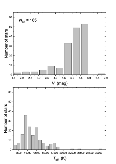
Figure 1: Histograms of the $V$ magnitudes (upper panel) and effective temperatures (lower panel) of our target star sample.

2 Data sources and target selection

We searched for all probable CP2 and CP4 stars in the most up-to-date collection, the most recent version of the General Catalogue of CP Stars published by Renson & Manfroid (2009). Because SMEI observed only bright, and hence for the most part well studied, stars (Fig. 1), the classifications in this catalogue should be reliable. However, we also included some borderline cases for which the spectral classification is not clear. Here we recall the remarks of Renson & Manfroid (2009) on the classification of CP stars: ”/” – a star improperly considered Ap or Am; ”?” – CP star of doubtful nature; and ”*” – well-known Ap or Am star. Although these classifications have to be viewed with caution, we excluded all stars denoted with a ”/”. In total, 165 stars were selected as our final sample. Essential data for these objects are given in Table 1.

The Solar Mass Ejection Imager (SMEI, Eyles et al., 2003) was launched into an Earth-terminator, Sun-synchronous, 840 km polar orbit as a secondary payload on board the Coriolis spacecraft in January 2003 and was terminated in September 2011. Its main purpose was to monitor and predict space weather in the inner solar system.

SMEI comprised three wide-field cameras, which were aligned such that the total field of view is a 180 deg and about 3 deg wide arc, yielding a near-complete image of the sky after about every 101.5 min orbit. The photometric passband ranges from 450 to 950 nm. Several papers (for example, Walczak et al., 2019; Zwintz et al., 2019) successfully employed the long time-baseline SMEI photometry for the study of variable stars.

A detailed description of the data analysis pipeline used to extract light curves from the raw data is provided by Hick et al. (2007). Stellar time series can be extracted from the SMEI website.

3 Time Series Analysis

The time series analysis described in this section was performed with the program packages PERANSO (Paunzen & Vanmunster, 2016) and VARTOOLS (Hartman & Bakos, 2016). For the identification of significant periods, the Generalized Lomb-Scargle algorithm (L-S, Zechmeister & Kürster, 2009) and the Phase-Dispersion Method (PDM, Stellingwerf, 1978) were applied. Both methods complement each other well, especially in the case of the SMEI data sets which are not free of various instrumental effects (Sect. 3.1).

The PDM algorithm is a classical string-length method. First of all, the data are folded on a series of trial periods. For each of these, the original data are assigned phases which are then re-ordered in ascending sequence. The reordered data are examined by inspection across the full phase interval between zero and one. For each trial period, the full phase interval is divided into a number of bins. Then, the sum of the lengths of line segments joining successive points (the string-length) is calculated. The variance of each of these bins is derived, giving a measure of the scatter around the mean light curve, defined by the means of the data in each sample. The PDM statistic is then calculated by dividing the overall variance of all the samples by the variance of the original (unbinned) data set. This process is repeated for each consecutive trial period. Minima in the plot of the string-length versus the trial period can be considered as corresponding to the underlying period.

The L-S algorithm is a variation of the Discrete Fourier Transform (DFT) which converts a finite list of equally spaced samples of a function (here the light curve) into a list of coefficients of a linear combination of sinusoidal and cosinusoidal functions. The data are transformed from the time to the frequency domain (Lomb-Scargle periodogram), invariant to time shifts. From a statistical point of view, the resulting periodogram is related to the $\chi^{2}$ for a least-squares fit of a single sinusoid to the data which can treat heteroscedastic measurement uncertainties. The underlying model is non-linear in frequency and the basis functions at different frequencies are not orthogonal.

For interpreting the significance of the detected periods, we used the False-Alarm probability (FAP), which denotes the probability that at least one out of $N$ independent power values in a prescribed search band of a power (or amplitude) spectrum computed from a white-noise time series is expected to be as large as or larger than a given value. Its correct interpretation has been often discussed in the literature (Horne & Baliunas, 1986; Cumming et al., 1999). Here, we consider a period significant if the $\log$ FAP value is larger than 1000. Furthermore, we require that this period is unambiguously detected with both the L-S and PDM methods. These are very strict limits that we feel justified to apply due to the characteristics of the SMEI light curves.

Figure 2: Histogram of detected instrumental periods in the range from 20 to 1000 days. Only periods detected more than two times are shown (there are none in the range from 600 to 1000 days). The panel in the right upper corner shows a typical L-S periodogram around the period of one day.

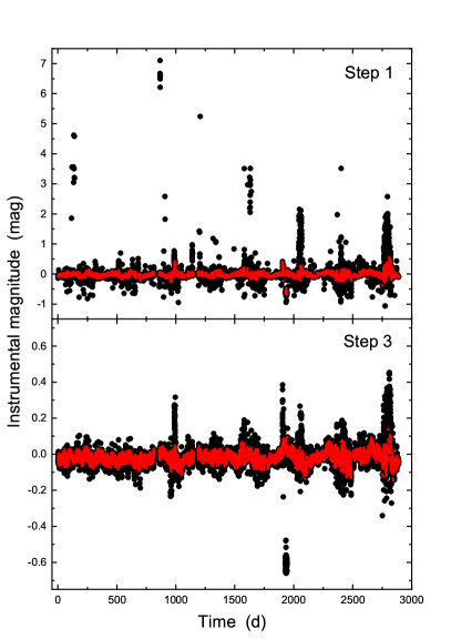
Figure 3: Example of the reduction steps one and three as described in Section 3.1. The light curve is that of the star HD 128898 ($\alpha$ Cir). Red dots denote magnitudes after the application of the corresponding reduction step.

3.1 Instrumental effects and data cleaning

SMEI light curves are strongly influenced by the Sun, Moon and daily cycles. The period range of ACV variables spans several magnitudes, extending from about half a day (Hümmerich et al., 2017) to hundreds or even thousands of years (Mathys, 2017). However, most ACV variables show periods of days (Netopil et al., 2017). Because of this, the SMEI orbital period of 101.5 min, which introduces artificial signals in the high frequency range, should not influence our results significantly.

To further investigate this matter, all 165 light curves were searched to identify the most important instrumentally-induced periods. The L-S algorithm was used to search for signals in the range from 20 to 1000 days, and the data were consecutively pre-whitened with the most significant periods, after which the L-S algorithm was applied again. This procedure was carried out five times.

In Fig. 2, we present the histogram (binned to one day intervals) of the derived instrumental periods. Only periods detected more than two times are shown; none were found in the range from 600 to 1000 days. In 111 out of the 165 light curves, the period around one year is the most significant one, followed by the half year period for an additional 47 light curves. Overall, we found significant peaks at around 52, 61, 73, 91, 122, 183, and 366 days. We also note the strong ”side lobes” of the one year period around 339 and 400 days. In addition, a one day period with a typical pattern is clearly visible in the periodograms (Fig. 2, upper right corner).

All cleaning and time series analysis steps are demonstrated using the light curve of HD 128898 ($\alpha$ Cir), which is a rapidly oscillating Ap (roAp) star that also shows low-amplitude ACV variations (Bruntt et al., 2009). Together with photometric data from the BRITE Constellation, TESS, and WIRE satellites, its SMEI light curve was used in the recent paper of Weiss et al. (2020) to study the spot structure of the star. Unfortunately, in their paper, the authors do not show amplitude spectra based on SMEI data (see Figs. 5 and 6 therein). The following automatic procedure was applied to all light curves.

• Step 1: cleaning of the raw light curve using a basic $\sigma$-clipping algorithm

• Step 2: consecutive prewhitening of the five periods with the highest FAP in the range from 50 to 1000 days and the one day period

• Step 3: cleaning of the residual light curve using a basic $\sigma$-clipping algorithm

• Step 4: search for significant periods

Fig. 3 illustrates the first and third steps graphically. It also highlights the strong instrumental trends present in the raw light curve.

Figure 4: Phased SMEI light curves of three sample stars with widely different periods and light curve characteristics.

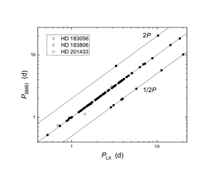
Figure 5: Comparison of the period values derived from SMEI data to the literature periods for our sample stars. Also indicated are the unity line and the lines correspondings to the half- and double-periods. Open symbols denote the three outliers (HD 183056, HD 183806, and HD 201433), which are discussed in the text.

Table 1: Significant periods of the 84 stars of our target star sample that show variability in the accuracy limit of the SMEI data, as based on the time-series analysis described in Section 3. Literature periods were gleaned from the International Variable Star Index (VSX, Watson et al., 2006) and the compilations of Netopil et al. (2017) and Jagelka et al. (2019). The typical period error amounts to 0.0001 d.

HD	$P_{\mathrm{SMEI}}$	$P_{\mathrm{Lit}}$	HD	$P_{\mathrm{SMEI}}$	$P_{\mathrm{Lit}}$	HD	$P_{\mathrm{SMEI}}$	$P_{\mathrm{Lit}}$	HD	$P_{\mathrm{SMEI}}$	$P_{\mathrm{Lit}}$
	(d)	(d)		(d)	(d)		(d)	(d)		(d)	(d)
3980	1.9758	3.9516	36485	2.8662	5.7325	96616	2.4292	2.4330	148112	3.0437	2.9510
10221	3.1538	3.1848	39317	2.6571	2.6569	103192	2.3567	2.3440	148898	2.9642	2.9900
11502	1.6091	1.6092	40312	3.6186	3.6187	108662	5.0761	5.0633	150549	3.7597	3.7600
12767	1.8923	1.8923	40394	14.3661	14.3680	109026	2.7280	2.7293	151525	4.1163	4.1160
14392	1.3086	1.3080	47144	2.2105	2.2100	112185	5.0889	5.0886	152107	3.8575	3.8567
15089	1.7403	1.7405	47152	2.7112	2.7112	118022	3.7225	3.7220	152564	2.1635	2.1637
18296	1.4421	2.8842	54118	3.2752	3.2753	120198	1.3858	1.3800	166596	1.6299	1.6700
19832	0.7279	0.7279	56022	0.9184	0.9183	124224	0.5207	0.5207	168733	6.3526	6.3000
21699	2.4920	2.4761	56455	2.0583	2.0580	125823	8.8166	8.8171	170000	1.7166	1.7165
22470	1.9289	1.9300	59256	0.9812	0.9430	128898	8.9051	0.0047	175362	3.6741	3.6740
22920	3.9471	3.9474	66624	1.9983	1.9984	130158	4.4142	4.4136	182255	1.2622	1.2600
23408	20.3234	10.2880	72968	5.6520	11.3050	131120	1.5687	1.5690	183056	0.7450	0.6870
25267	1.2099	1.2094	73340	2.6676	2.6675	133880	0.8775	0.8775	183806	3.1197	2.9210
25823	7.2267	7.2274	74067	3.1129	3.1130	134759	1.5566	3.0993	196178	1.0041	1.0060
26961	1.5274	1.5274	74521	7.0519	6.9071	137909	18.2751	18.4870	196502	10.1376	20.2750
27309	1.5689	1.5690	74560	1.5509	1.5511	138764	1.2586	1.2588	201433	1.1260	1.4289
28843	1.3738	1.3740	77653	1.4878	1.4878	138769	2.0895	2.0894	201834	3.5351	3.5354
29009	3.8002	3.8200	79158	1.9174	3.8340	140160	1.5958	1.5958	209515	2.3870	2.3880
29305	2.9432	2.9500	82984	6.0878		140728	1.2956	1.3049	220825	1.4149	1.4150
32549	4.6396	4.6397	92664	1.6731	1.6680	142096	6.6411	3.3136	221006	2.3148	2.3148
32650	2.7350	2.7348	93030	2.2031	2.2027	142990	0.9789	0.9789	223640	3.7350	3.7352

3.2 Variable stars

In total, we identified 84 variable stars, from which 83 have periods in the International Variable Star Index (VSX, Watson et al., 2006) of the American Association of Variable Star Observers and the compilations of Netopil et al. (2017) and Jagelka et al. (2019). Example phased light curves of three sample stars (HD 11502, HD 25823, and HD 74067) are shown in Figure 4. The different light curves characteristics relating to the spot distribution on the surfaces are nicely visible.

In Fig. 5, we present a comparison of the here derived periods to the literature periods of the stars listed in Table 1. The typical period error amounts to 0.0001 d. Because in orientations where two spots come into view during a star’s rotation cycle, a significant number of ACV variables exhibit double-waved light curves (Hümmerich et al., 2016). Therefore, a twice longer (or shorter) rotation period is sometimes possible, in particular for objects with very small amplitudes and/or significant scatter in their light curves. We emphasise that the given period values correspond to the periods with the highest FAP values; nevertheless, the most prominent periods may sometimes represent harmonics of the true rotation period, as becomes obvious from Fig. 5. In ambiguous cases, the true period has to be determined by other means such as radial velocity studies.

One object (HD 82984) is listed as ”CST:” in the VSX, that is, as a non-variable (constant) star, which was formerly suspected to be a variable. This classification goes back to Jerzykiewicz & Sterken (1977), who did not discuss HD 82984 in more detail. No further references to a photometric time-series study of this object were found in the literature; we are therefore confident that the here presented solution is the first published period of this star.

There are three obvious outliers in Fig. 5, which are discussed in more detail below.

HD 183056: Williams et al. (1974) reported variability of the H$\beta$-line profile on the basis of 49 scans taken during a time span of 188 min. Later on, Winzer (1974) reported a possible period of 0.68674 d for this star, whereas Adelman & Pyper (1993b) concluded that if variability is present, the amplitude has to be below 0.02 mag. HD 183056 was included in the Hipparcos-based study of Adelman (1998); however, no period solution was presented.

HD 183806: Mathys & Manfroid (1985) measured this star in Strömgren $uvby$ filters and reported a possible period of 2.9213 d. No other period information on this star seems to have been published. The here derived SMEI period of 3.1197 d is slightly longer than the published one.

HD 201433: This is a single-lined spectroscopic triple system consisting of a massive Slowly Pulsating B (SPB) star orbited by two low-mass stars with periods of about 3.31 and 154 d, respectively (Kallinger et al., 2017). The amplitude spectrum of the SMEI data is clearly indicative of multiperodicity due to pulsations. The here detected periods (not all listed in Table 1) are compatible with those listed in Table 4 of Kallinger et al. (2017).

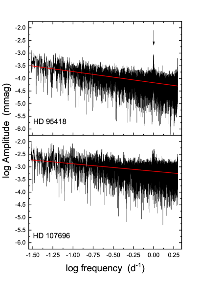
Figure 6: Logarithmic amplitude spectra of the SMEI light curves of HD 95418 (upper panel) and HD 107696 (lower panel). Also shown are the fits with the parameters listed in Table 2. In both amplitude spectra, the remains of the one-day frequency is clearly visible.

All other stars lie well on the correlations presented in Fig. 5, which lends confidence in our time-series analysis.

Table 2: Results from fitting the amplitude spectra (Fig. 6) of the apparently constant stars in the form $\log A=a+b\log f$, where $A$ is the amplitude and $f$ the frequency. Throughout the sample, the errors relating to the parameters $a$ and $b$ amount to 0.002 and 0.005, respectively

HD	$a$	$b$	HD	$a$	$b$	HD	$a$	$b$	HD	$a$	$b$
1280	$-$3.944	$-$0.461	64740	$-$3.976	$-$0.414	108945	$-$3.723	$-$0.448	181615	$-$3.722	$-$0.550
2054	$-$3.765	$-$0.445	68351	$-$3.563	$-$0.458	115735	$-$3.901	$-$0.443	182568	$-$3.824	$-$0.454
4853	$-$3.840	$-$0.492	68601	$-$3.990	$-$0.475	116458	$-$3.794	$-$0.335	185872	$-$3.468	$-$0.439
5737	$-$3.837	$-$0.431	71046	$-$3.893	$-$0.317	116656	$-$4.100	$-$0.466	187474	$-$3.634	$-$0.431
6397	$-$3.678	$-$0.471	77350	$-$3.612	$-$0.446	120640	$-$3.454	$-$0.419	188041	$-$3.587	$-$0.380
11753	$-$3.806	$-$0.424	78556	$-$3.526	$-$0.404	120709	$-$3.841	$-$0.490	189178	$-$3.822	$-$0.461
18519	$-$3.950	$-$0.479	78702	$-$3.677	$-$0.370	123255	$-$3.709	$-$0.478	196524	$-$3.990	$-$0.449
19400	$-$3.798	$-$0.331	79416	$-$3.638	$-$0.452	124425	$-$3.755	$-$0.436	198667	$-$3.708	$-$0.407
23850	$-$3.769	$-$0.449	81188	$-$4.092	$-$0.361	128974	$-$3.472	$-$0.464	201601	$-$3.897	$-$0.442
28319	$-$3.858	$-$0.451	90264	$-$3.829	$-$0.370	130109	$-$3.914	$-$0.445	202444	$-$4.050	$-$0.437
30612	$-$3.717	$-$0.333	90972	$-$3.534	$-$0.428	135382	$-$3.918	$-$0.314	202627	$-$3.854	$-$0.461
34968	$-$3.920	$-$0.479	92728	$-$3.666	$-$0.374	136933	$-$3.498	$-$0.449	202671	$-$3.608	$-$0.430
35039	$-$3.925	$-$0.437	94334	$-$3.934	$-$0.417	143699	$-$3.668	$-$0.440	203006	$-$3.758	$-$0.448
35497	$-$4.037	$-$0.463	95418	$-$4.169	$-$0.439	148330	$-$3.917	$-$0.456	203585	$-$3.453	$-$0.450
38104	$-$3.872	$-$0.435	96097	$-$3.675	$-$0.552	152127	$-$3.690	$-$0.414	205637	$-$3.630	$-$0.424
42509	$-$3.413	$-$0.468	97633	$-$3.961	$-$0.487	157740	$-$3.480	$-$0.424	206742	$-$3.916	$-$0.504
55719	$-$3.932	$-$0.444	98664	$-$3.674	$-$0.557	169467	$-$3.813	$-$0.439	215766	$-$3.213	$-$0.407
59635	$-$3.743	$-$0.472	101189	$-$3.607	$-$0.378	172728	$-$3.783	$-$0.476	221760	$-$3.768	$-$0.445
61110	$-$3.828	$-$0.472	106661	$-$3.687	$-$0.510	175156	$-$3.736	$-$0.403
61641	$-$3.706	$-$0.429	107696	$-$3.172	$-$0.295	177003	$-$3.779	$-$0.400
64486	$-$3.980	$-$0.505	108283	$-$3.723	$-$0.473	177756	$-$4.003	$-$0.470

3.3 Apparently constant stars

Here, we define ”constant” as light curves whose amplitude spectra show no significant peaks as defined in Section 3. As first step, we describe the characteristics of the amplitude spectra in more detail.

The noise in the amplitude spectra can be well described as 1/f or ”flicker” noise. Sometimes it also referred to as ”pink” noise (Subba Rao et al., 1997). It can be described as a linear law by plotting the logarithm of the frequency ($f$) versus the logarithm of the amplitude ($A$).

$$\log A=a+b\log f.$$ (1)

The $a$ and $b$ values of the 81 amplitude spectra without any significant peaks are listed in Table 2. The errors of the parameters $a$ and $b$ amount to 0.002 and 0.005, respectively, throughout the sample, which implies that the estimates are very robust. The mean slope for the complete sample is $-$0.44(5), which means that the noise characteristics are not dependent on the individual data sets. The level of the noise characterised by the intercept depends on the number of data points and the magnitude of the stars (photon statistics).

In Fig. 6, we present example amplitude spectra of two stars showing, respectively, a low (HD 95418, upper panel) and a high (HD 107696, lower panel) noise level in the investigated frequency domain. The fits are shown as straight lines. In both amplitude spectra, the remains of the one-day frequency are clearly visible.

Figure 7: Comparison of the parallaxes from the Hipparcos catalogue to the Gaia EDR3 parallaxes (upper panel) and the Gaia DR2 parallaxes (lower panel). Several obvious outliers are visible in both plots.

From the 81 stars without any significant signals in SMEI data, 18 stars have periods in the literature and another 10 stars are flagged as variables or variable star candidates in the VSX. In the following, we discuss these objects in more detail.

In the case of four stars, the literature period exceeds 30 days, which may explain their non-detection in SMEI data: HD 116458 (149.25373 d), HD 181615 (137.9343 d), HD 187474 (2300 d), and HD 188041 (224.5 d).

Wraight et al. (2012) identified low amplitude variations on the basis of STEREO data in HD 6397, HD 68351, and HD 77350.

One of the most valuable sources for the study of bright ACV variables are the data of the Hipparcos mission. Adelman (1998) and Paunzen & Maitzen (1998) reported low amplitude variability in HD 73340, HD 79416, HD 201601, HD 202671, HD 203006, HD 205637, and HD 221760.

HD 5737: the amplitude of this He-weak object amounts to only a few mmags in the Strömgren photometric system (Manfroid & Renson, 1994).

HD 23850: this star was found constant in light by Wraight et al. (2012).

HD 28319: this is the binary system $\theta^{2}$ Tauri, the brightest member of the Hyades, which consists of at least two components showing $\delta$ Scuti-type pulsations (Armstrong et al., 2006). The existence of rotational variability was never confirmed.

HD 35039: Balona & Engelbrecht (1985) found first evidence for line-profile variations in this star using a limited set of observations. Later on, Le Contel et al. (2001) classified HD 35039 as a SPB star showing multiperiodic radial velocity variations. However, it is a He-rich CP star according to Romanyuk et al. (2013). This object deserves a new thorough analysis of all spectroscopic data to shed more light on its nature.

HD 68601: this star was found variable by Jerzykiewicz & Sterken (1977), who did not discuss its characteristics in more detail. No other variability study of this object was found in the literature.

HD 107696: this star was part of the long-term photometric survey of variable stars at ESO (Manfroid et al., 1991). However, no detailed results were published on this object by the consortium.

HD 108945: this star was analysed in more detail with photometric and spectroscopic data by Paunzen et al. (2019), who confirmed the existence of rotational light variability but were unable to find any significant frequencies with a semi-amplitude exceeding 0.2 mmag in the high-frequency range.

HD 115735: this is a well-studied ACV variable (Zverko, 1984; Zverko et al., 1994).

HD 124425: no time-series analysis was found in the literature.

HD 148330: Ziznovsky (1983) identified radial velocity variations and photometric variability with an amplitude of 17 mmag in the $g_{2}$ filter (Paunzen et al., 2005).

HD 215766: this star was found constant by Wraight et al. (2012).

Upper limits of variability were derived for 50 out of 165 objects ($\sim$30%) for which no entry about variability exists in the VSX and the literature. The question arises which parameters define the boundary conditions for the occurrence of ACV variability, that is, the presence of spots of sufficient size or contrast on the surface that lead to observable photometric variations.

Jackson & Jeffries (2013) analysed the relationship between size and surface coverage of starspots on magnetically-active low-mass stars. Employing different filling factors, characteristic scalelengths, and spot distributions in their simulations, they were able to show that small light-curve amplitudes in magnetically active M dwarfs can be explained by a starspot model consisting of large filling factors of dark spots with a random distribution on the stellar surface. To adjust this model to higher mass objects and use it for a comparison with the observations, a much larger sample size of non-variable CP2/4 stars is needed. Although a huge amount of high-quality photometric light curves are available today, such a project – although being of great interest – is not easy to implement (Paunzen et al., 2020).

4 Astrophysical parameters and the Hertzsprung-Russell-diagram

In this section, we describe the sources and methods used to create the Hertzsprung-Russell diagram for our target star sample.

Photometry: photometric data of the Johnson $UBV$ and Geneva 7-colour systems were taken from the General Catalogue of Photometric data and the All-Sky Compiled Catalogue of 2.5 million stars (ASCC, Kharchenko, 2001), whereas the Strömgren-Crawford $uvby\beta$ indices were gleaned from the catalogue by Paunzen (2015).

No Johnson $(U-B)$ colours are available for HD 3980, HD 18519, HD 54118, HD 59635, HD 166596, HD 168733, and HD 183806. The full set of Strömgren-Crawford $uvby\beta$ indices was measured for all objects, except for HD 4853. Geneva 7-colour photometry is not available for HD 21699, HD 23408, HD 108662, HD 108945, HD 172728, HD 177003, HD 182568, HD 185872, and HD 189178.

Reddening: as was shown by Netopil et al. (2008), the commonly employed dereddening procedures published by Napiwotzki et al. (1993) are also applicable to CP2/4 stars. They were therefore used for the reddening estimation of all objects except HD 4853, in which case we used the reddening map by Green et al. (2019), which is based on Gaia parallaxes and stellar photometry from Pan-STARRS 1 and 2MASS. Because this star is located in the solar vicinity (distance of 82 pc), the reddening is negligible.

For the calibrations of the different photometric systems, we used the following relations (Paunzen et al., 2006):

$$A_{V}=3.1E(B-V)=4.3E(b-y)=4.95E(B2-V1).$$ (2)

A value of 0.01 mag in $E(b-y)$ was adopted for all objects.

Bolometric correction: we used the correlation given by Netopil et al. (2008), which was tailored for the use with CP stars.

Luminosity: today, regarding bright stars, we are in the lucky position to have parallaxes available from both the Hipparcos (van Leeuwen, 2007) and the Gaia (Gaia Collaboration et al., 2018; Lindegren et al., 2018; Gaia Collaboration et al., 2020) space missions. Because our sample consists of stars between magnitudes 1.5 and 7 (Fig. 1), we checked the consistency of both data sources. Only HD 36485 has no parallax listed in the Hipparcos catalogue, whereas measurements for 11 stars (HD 29305, HD 35497, HD 77653, HD 81188, HD 93030, HD 96097, HD 103192, HD 116656, HD 170000, HD 196524, and HD 203585) and 16 stars (HD 29305, HD 35497, HD 40312, HD 77653, HD 81188, HD 93030, HD 96097, HD 97633, HD 103192, HD 112185, HD 116656, HD 134759, HD 170000, HD 196524, HD 202444, and HD 203585) are missing in the Gaia DR2 and EDR3, respectively.

In Fig. 7, we present the comparison of the parallaxes from the Hipparcos and Gaia data releases. In general, the agreement is very good, but some outliers are present. We have checked the available literature to search for reasons to account for these discrepancies. Most likely, binarity or circumstellar envelopes are at the root of the observed outlying positions, but it is out of the scope of this paper to investigate this issue in detail and to decide which of the parallax sources is the most reliable one.

Parallaxes were used in the sequence EDR3, DR2, and Hipparcos, depending on their availability. The parallax values were used to calculate the final luminosities listed in Table 1; a full error propagation was applied.

$Gaia$ DR2 also includes luminosities for objects with effective temperatures less than 10 000 K (Cochetti et al., 2020). Corresponding luminosities were obtained for 15 stars from our list. A comparison of the Gaia DR2 luminosities to our values is provided in Figure 8, from which it is obvious that the Gaia DR2 luminosities are systematically too low and should be used with caution for CP2/4 stars.

Figure 8: Comparison of the luminosities derived in this work and the Gaia DR2 catalogue. The latter appear systematically too low.

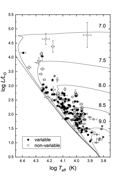
Figure 9: Positions of our target stars in the Hertzsprung-Russell diagram, which is provided in the form of $\log T_{\mathrm{eff}}$ versus $\log L/L_{\odot}$ (Table 1). Also shown are stellar evolutionary models for the indicated logarithmic ages by Ekström et al. (2012).

Effective temperature: if available, data from the Johnson $UBV$, Geneva 7-colour, and Strömgren-Crawford $uvby\beta$ photometric systems were used. Netopil et al. (2008) introduced calibrations for CP stars using individual corrections for the temperature domain and the CP subclass, which are summarised in their Table 2. We here follow their approach. For the derivation of the final effective temperatures, all calibrated values were averaged and the standard deviations were calculated.

Mass and Evolutionary Phase: to estimate these parameters, we employed the Stellar Isochrone Fitting Tool, which builds on the methodology of Malkov et al. (2010) in estimating the mass, age, radius, and evolutionary phase of a star according to its effective temperature and luminosity. The tool automatically searches for similar data in models based on evolutionary tracks and selects the four grid points closest to the input value in the Hertzsprung-Russell diagram. From these grid points, the output parameters are obtained by repetitive linear interpolation.

The final astrophysical parameters are listed in Table 1. In Fig. 1 (lower panel), the distribution of the effective temperatures is shown. Most stars have values between 9 000 and 13 000 K, which corresponds to spectral types between A2 and B8, in agreement with the peak distribution of CP stars. As expected, there is also an extension to cooler and hotter temperatures that covers the whole range of the CP star phenomenon.

In Fig. 9, the Hertzsprung-Russell diagram is presented together with non-rotating isochrones from Ekström et al. (2012) for [Z] = 0.014. The choice of the metallicity rests on the analysis presented in Sect. 4.2.2. of Hümmerich et al. (2020). It is based on published individual abundances for stars of our target star sample. No object is located below the zero-age main sequence, but several stars are close to the terminal-age main sequence, which implies that they are past the core-hydrogen burning stage and do not belong to luminosity class V. The most significantly deviating object is HD 68601. It was classified as ApSr on the basis of S2/68 UV spectra by Cucchiaro et al. (1978). Later on, it was classified as A5 Ib by Gray & Garrison (1989), which is compatible with its location in the Hertzsprung-Russell diagram as shown in Fig. 9. The $\Delta$a value, which provides a measure of peculiarity by an estimation of the 5200 Å flux depression, is slightly positive (+10 mmag, Vogt et al., 1998). Unfortunately, no detailed elemental abundance studies are available in the literature. Spectroscopic studies of this interesting and apparently evolved star are encouraged.

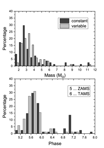
Figure 10: Histograms of the masses and evolutionary phases of the constant and variable CP2/4 stars. The coding of the evolutionary phase follows the isochrone grid of Bressan et al. (2012).

Figure 10 shows the mass and evolutionary status of the sample divided into variable (Table 1) and constant (Table 2) stars. The coding for the evolutionary status was taken from the isochrone grid by Bressan et al. (2012). The mass distribution peaks at about three solar masses, as expected from the effective temperature distribution (Figure 1). Interestingly, variable stars show significantly higher masses than constant ones. This is expected because high-mass CP2/4 stars usually have He and Si spots, which are known to produce higher-amplitude variations than Sr, Cr, or Eu spots.

The age distribution is similar to the distributions of the fainter ACV variables investigated by Bernhard et al. (2015); Hümmerich et al. (2016); Bernhard et al. (2020). There is a conspicuous lack of young stars close to or at the zero-age main sequence. Almost all objects have ages between 100 Myr and 1 Gyr (Figure 9), which still places them on the main sequence but already significantly above the zero-age main sequence line. Variable stars seem to be in a more advanced evolutionary status than the constant ones. This information is important for theories dealing with the origin of the observed magnetic fields in these objects. Over the last years, a body of evidence has been built up which strongly favours the fossil field theory, which postulates that the magnetic fields are relics of the ”frozen-in” interstellar magnetic field (Braithwaite & Cantiello, 2013). Our results imply that spots on the stellar surface, which are thought to be coupled to the magnetic field strength, only appear after the star has spent some time on the main-sequence. From studies of open clusters (Bagnulo et al., 2003; Pöhnl et al., 2003; Landstreet et al., 2008), it has been established that young CP2/4 stars exist, although they seem to be rare. Young CP2/4 stars are present in the large sample of stars published by Hümmerich et al. (2020), although they are conspicuously underrepresented. The reasons for the observed uneven distribution of CP2/4 stars are still unresolved and a matter of debate.

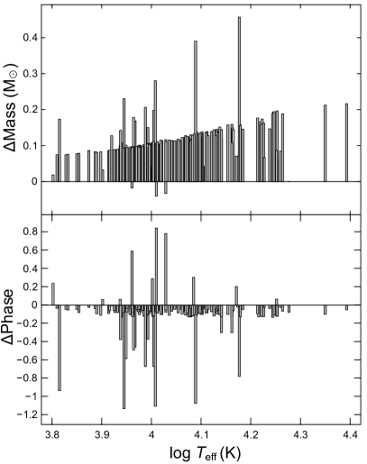
Figure 11: Differences of mass and evolutionary phase estimated from tracks with [Z] = 0.020 and [Z] = 0.014.

Finally, we checked the influence of the metallicity on the mass and evolutionary phase distribution. For this, we used an identical isochrone grid for [Z] = 0.020 and calibrated the target star sample as described above. In Fig. 11, the differences of mass and evolutionary phase in the sense ”0.020 $-$ 0.014” is shown. Derived masses are between 0.1 and 0.2 $M_{\odot}$ larger for the higher metallicity, which is well below 5% for the investigated mass range (Fig. 10). The evolutionary phase is constantly about 0.1 smaller in the sense that higher metallicity results in younger ages. Again, these absolute differences are negligible when compared to the observational uncertainties and possible effects such as unknown binarity. The bin size used for the analysis presented in Fig. 10 is 0.2 for the evolutionary phase. About 10% of the stars from our sample do not follow the general trend. These are the objects situated close to, or slightly above, the terminal-age main sequence. The observed sudden ”jump” with the isochrone’s metallicity is due to the corresponding shift in luminosity for the same effective temperature, which decides whether these objects are still calibrated as core hydrogen-burning objects or not.

5 Conclusions

Using SMEI data, we investigated the light curves of 165 CP2 and CP4 stars and candidates selected from the catalogue by Renson & Manfroid (2009). Because of the presence of strong instrumental trends, a basic cleaning algorithm was introduced, and instrumentally-introduced frequencies were identified and subtracted from the data sets in an automated way.

The time series analysis was performed using the Generalized Lomb-Scargle algorithm and the Phase-Dispersion Method. Because both methods complement each other and are sensitive to the different light curve characteristics and instrumental effects, this approach was found to work well with SMEI data and to derive the most reliable results.

Apart from performing thorough time-series analyses, it is also important to establish criteria defining constancy. We found that the noise of the amplitude spectra can be well described as flicker (or pink) noise, which, when plotting the logarithm of the frequency versus the logarithm of the amplitude, is characterised by a linear law that describes the mean noise level over the investigated frequency domain. Corresponding parameters for all apparently constant stars were presented.

In total, we processed and analysed 165 individual light curves from which 84 show variability in the accuracy limit of the SMEI data. We compared the derived periods with published literature values and found an excellent agreement, which proves that SMEI data are well suited to the long-term study of ACV variables.

As last step, we used calibrations specifically developed for CP stars as well as Hipparcos and Gaia data to estimate the effective temperatures and luminosities for our target star sample. Masses and evolutionary stages were calibrated using an appropriate isochrone grid. The derived astrophysical parameters provide a coherent picture of ACV variables being concentrated towards the end of their main-sequence lifetime. Our mass estimates support that He and Si peculiarities – preferentially found in the hotter, and thus more massive, CP stars – produce larger spots or spots of higher contrast.

SMEI data fill an important gap in time in the observation of bright ACV variables, for which follow-up spectroscopic and spectropolarimetric observations are comparatively easy to achieve. The here presented results are therefore important for the future analysis and, in particular, the study of the long-term behaviour of CP2/4 star light curves, and will benefit future studies of these fascinating objects.

Data availability

The data underlying this article will be shared on reasonable request to the corresponding author.

Appendix A Essential data for our sample stars

Table 1 lists essential data for our sample stars. It is organised as follows:

• Column 1: HD number.

• Column 2: Identifier from Renson & Manfroid (2009).

• Column 3: Right ascension (J2000). Positional information was taken from GAIA DR2 (Gaia Collaboration et al., 2018; Lindegren et al., 2018).

• Column 4: Declination (J2000).

• Column 5: Spectral classification from Renson & Manfroid (2009).

• Column 6: Mean $V$ magnitude.

• Column 7: Mean $V$ magnitude error.

• Column 8: Parallax (Hipparcos).

• Column 9: Parallax error.

• Column 11: Parallax (Gaia DR2).

• Column 11: Parallax error.

• Column 12: Parallax (Gaia EDR3).

• Column 13: Parallax error.

• Column 14: Absorption in the $V$ band.

• Column 15: Mean effective temperature.

• Column 16: Mean effective temperature error.

• Column 17: Luminosity.

• Column 18: Luminosity error.

• Column 19: Mass.

• Column 20: Evolutionary Phase.

Table 1: Essential data for our sample stars, sorted by increasing right ascension. The columns denote: (1) HD number. (2) Identifier from Renson & Manfroid (2009). (3) Right ascension (J2000; GAIA DR2). (4) Declination (J2000; GAIA DR2). (5) Spectral classification from Renson & Manfroid (2009). (6) Mean $V$ magnitude. (7) Mean $V$ magnitude error. (8) Parallax (Hipparcos). (9) Parallax error. (10) Parallax (Gaia DR2). (11) Parallax error. (12) Parallax (Gaia EDR3). (13) Parallax error. (14) Absorption in the $V$ band. (15) Mean effective temperature. (16) Mean effective temperature error. (17) Luminosity. (18) Luminosity error. (19) Mass. (20) Evolutionary Phase.

(1) (2) (3) (4) (5) (6) (7) (8) (9) (10) (11) (12) (13) (14) (15) (16) (17) (18) (19) (20) HD ID_RM09 RA(J2000) Dec(J2000) SpT_RM09 $V$ mag e_$V$ mag $\pi$ (Hip) e_$\pi$ (Hip) $\pi$ (DR2) e_$\pi$ (DR2) $\pi$ (EDR3) e_$\pi$ (EDR3) $A_{V}$ $\log T_{\mathrm{eff}}$ e_$\log T_{\mathrm{eff}}$ $\log L/L_{\odot}$ e_$\log L/L_{\odot}$ Mass Phase 1280 270 00 17 05.496 +38 40 53.91 A2 Si Sr 4.607 0.005 10.56 0.96 15.685 0.383 18.875 0.425 0.000 3.944 0.014 1.67 0.02 2.16 5.65 2054 490 00 25 06.402 +53 02 48.36 B9 Si 5.760 0.010 6.32 0.33 5.839 0.138 5.059 0.142 0.088 4.053 0.008 2.26 0.02 3.43 5.84 3980 1090 00 41 46.399 $-$56 30 04.83 A7 Sr Eu Cr 5.698 0.003 14.92 0.35 14.613 0.090 14.770 0.041 0.000 3.914 0.005 1.28 0.01 1.91 5.57 4853 1280 00 54 53.111 +83 42 26.60 A3 Si 5.607 0.015 11.40 0.61 12.158 0.110 12.826 0.076 0.000 3.932 0.009 1.48 0.01 2.08 5.63 5737 1490 00 58 36.358 $-$29 21 26.63 B6 He wk. 4.310 0.010 4.20 0.18 4.707 0.423 4.622 0.191 0.015 4.141 0.005 3.21 0.08 5.40 6.48 6397 1637 01 05 05.356 +14 56 45.68 F3 Sr 5.700 0.010 18.32 0.32 19.028 0.128 18.941 0.067 0.000 3.828 0.022 1.15 0.01 1.73 5.85 10221 2550 01 42 20.514 +68 02 34.85 A0 Si Sr Cr 5.576 0.019 8.39 0.50 7.682 0.113 7.696 0.057 0.002 4.029 0.015 2.02 0.02 2.86 5.68 11502 2930 01 53 31.814 +19 17 38.13 A1 Si Cr Sr 3.880 0.000 19.88 0.96 19.983 0.346 19.627 0.153 0.000 3.997 0.015 1.81 0.02 2.57 5.66 11753 3010 01 54 22.018 $-$42 29 48.89 A0 Hg Pt 5.108 0.005 10.63 0.37 10.483 0.247 10.185 0.189 0.000 3.998 0.004 1.88 0.02 2.67 5.73 12767 3260 02 04 29.434 $-$29 17 48.47 A0 Si 4.686 0.005 8.79 0.26 9.616 0.263 9.403 0.133 0.000 4.112 0.011 2.36 0.02 3.62 5.60 14392 3620 02 20 58.201 +50 09 05.44 B9 Si 5.550 0.010 8.31 0.34 7.899 0.109 8.528 0.168 0.009 4.069 0.020 2.09 0.01 3.01 5.45 15089 3760 02 29 03.941 +67 24 08.46 A4 Sr 4.503 0.026 24.55 0.81 21.960 0.333 22.080 0.118 0.000 3.927 0.011 1.41 0.02 2.04 5.63 18296 4560 02 57 17.278 +31 56 03.30 A0 Si Sr 5.102 0.004 10.20 0.27 9.848 0.258 9.345 0.132 0.090 4.041 0.009 2.05 0.02 2.99 5.69 18519 4630 02 59 12.719 +21 20 25.09 A3 Ti 5.556 0.008 9.81 0.79 8.511 0.342 9.030 0.185 0.000 3.944 0.014 1.82 0.04 2.43 5.82 19400 4850 03 02 15.449 $-$71 54 09.04 B8 He wk. 5.520 0.007 6.34 0.20 6.536 0.099 6.500 0.062 0.000 4.132 0.003 2.41 0.01 3.77 5.51 19832 4910 03 12 14.248 +27 15 25.08 B8 Si 5.727 0.090 6.49 0.76 8.041 0.172 7.867 0.065 0.038 4.088 0.013 2.06 0.04 3.14 5.36 21699 5410 03 32 08.596 +48 01 24.58 B8 He wk. Si 5.465 0.004 5.39 0.31 5.912 0.151 5.638 0.154 0.146 4.178 0.009 2.70 0.02 4.52 5.59 22470 5710 03 36 17.393 $-$17 28 01.55 B9 Si 5.222 0.004 6.70 0.51 7.646 0.329 8.501 0.468 0.000 4.102 0.011 2.32 0.04 3.40 5.51 22920 5840 03 40 38.335 $-$05 12 38.57 B8 Si 5.529 0.014 6.57 0.47 5.352 0.169 5.240 0.092 0.031 4.131 0.009 2.59 0.03 4.05 5.72 23408 6000 03 45 49.602 +24 22 03.72 B7 He wk. Mn 3.869 0.003 8.51 0.28 9.478 0.683 7.671 0.310 0.156 4.104 0.006 2.75 0.06 4.57 6.11 23850 6100 03 49 09.744 +24 03 12.15 B8 He wk. 3.621 0.003 8.53 0.39 8.429 0.556 8.118 0.479 0.107 4.085 0.008 2.88 0.06 4.40 6.81 25267 6440 03 59 55.478 $-$24 00 58.79 A0 Si 4.645 0.015 9.96 0.22 10.665 0.211 9.974 0.100 0.000 4.076 0.010 2.20 0.02 3.32 5.67 25823 6560 04 06 36.408 +27 35 59.51 B9 Sr Si 5.194 0.005 7.76 0.36 8.205 0.169 8.067 0.106 0.000 4.102 0.010 2.27 0.02 3.44 5.54 26961 6880 04 18 14.605 +50 17 43.81 A2 Si 4.592 0.003 10.40 0.35 9.558 0.763 8.547 0.234 0.000 3.961 0.011 2.12 0.07 3.00 6.24 27309 7010 04 19 36.695 +21 46 24.68 A0 Si Cr 5.380 0.010 10.00 0.28 11.142 0.204 11.402 0.095 0.000 4.075 0.011 1.87 0.02 2.85 5.10 28319 7240 04 28 39.716 +15 52 15.12 A8 Sr 3.398 0.004 21.69 0.46 20.835 0.373 21.813 0.374 0.016 3.902 0.012 1.90 0.02 2.40 7.07 28843 7380 04 32 37.560 $-$03 12 34.39 B9 He wk. Si 5.799 0.020 6.86 0.35 5.903 0.114 5.896 0.061 0.053 4.162 0.006 2.49 0.02 4.05 5.36 29009 7420 04 33 54.733 $-$06 44 20.10 B9 Si 5.713 0.004 3.94 0.52 3.722 0.127 4.181 0.076 0.000 4.091 0.007 2.73 0.03 3.94 5.86 29305 7490 04 33 59.785 $-$55 02 42.10 A0 Si 3.262 0.004 19.34 0.31 0.034 4.064 0.002 2.22 0.01 3.23 5.70 30612 7940 04 43 03.948 $-$70 55 51.79 B9 Si 5.523 0.006 6.64 0.23 6.841 0.075 6.970 0.063 0.006 4.094 0.008 2.28 0.01 3.39 5.58 32549 8280 05 04 34.140 +15 24 15.01 B9 Si Cr 4.680 0.010 8.93 0.24 9.343 0.394 7.807 0.140 0.000 3.996 0.013 2.15 0.04 3.14 6.25 32650 8350 05 12 22.433 +73 56 47.93 B9 Si 5.447 0.005 8.63 0.47 10.529 0.228 8.935 0.230 0.000 4.062 0.011 1.86 0.02 2.97 5.48 34968 8933 05 20 26.906 $-$21 14 22.91 B9 He var. 4.703 0.005 7.84 0.51 8.719 0.166 7.822 0.112 0.000 4.005 0.010 2.21 0.02 3.08 6.56 35039 8953 05 21 45.751 $-$00 22 56.87 B2 He 4.729 0.012 3.51 0.49 2.867 0.351 2.859 0.158 0.128 4.277 0.012 3.88 0.11 8.00 7.08 35497 9110 05 26 17.514 +28 36 27.12 B8 Cr Mn 1.650 0.008 24.36 0.34 0.000 4.098 0.014 2.73 0.01 4.17 5.90 36485 9440 05 32 00.413 $-$00 17 04.19 B2 He 6.847 0.022 2.573 0.077 2.625 0.054 0.135 4.246 0.009 3.05 0.03 5.57 5.46 38104 10240 05 45 54.039 +49 49 34.56 A1 Cr Eu 5.461 0.010 7.89 0.84 5.560 0.199 8.188 0.264 0.000 3.959 0.010 2.24 0.03 2.60 5.85 39317 10560 05 52 22.300 +14 10 18.45 B9 Si Eu Cr 5.550 0.010 7.69 0.29 7.143 0.176 6.855 0.096 0.000 3.991 0.011 2.02 0.02 2.85 5.85 40312 10750 05 59 43.245 +37 12 45.28 A0 Si 2.645 0.029 19.70 0.16 17.183 0.411 0.000 4.010 0.013 2.45 0.02 3.33 6.91 40394 10790 06 00 58.568 +47 54 06.94 A0 Si Fe 5.732 0.024 2.82 0.47 3.588 0.127 3.155 0.082 0.185 4.003 0.012 2.64 0.03 3.86 7.23 42509 11320 06 12 01.340 +19 47 26.00 B9 Si 5.770 0.010 3.92 0.47 3.030 0.189 3.086 0.209 0.000 4.000 0.010 2.69 0.05 3.66 7.19 47144 12660 06 35 24.175 $-$36 46 47.54 B9 Si 5.590 0.000 6.40 0.35 5.924 0.074 6.264 0.062 0.000 4.102 0.016 2.40 0.01 3.53 5.62 47152 12670 06 38 23.003 +28 59 03.81 A0 Eu Cr Hg 5.759 0.043 9.41 0.62 8.514 0.137 8.274 0.157 0.129 3.992 0.010 1.84 0.02 2.61 5.72 54118 14860 07 04 18.331 $-$56 44 59.02 A0 Si 5.151 0.002 10.84 0.43 11.683 0.182 10.363 0.175 0.000 4.009 0.020 1.79 0.01 2.67 5.66 55719 15140 07 12 15.790 $-$40 29 55.66 A3 Sr Cr Eu 5.302 0.004 7.93 0.38 7.496 0.152 7.564 0.095 0.000 3.945 0.013 2.03 0.02 2.60 7.05 56022 15250 07 13 13.359 $-$45 10 57.84 A0 Si Cr Sr 4.857 0.074 17.69 0.14 17.455 0.131 17.362 0.077 0.000 3.985 0.006 1.52 0.03 2.27 5.40 56455 15400 07 14 46.009 $-$46 50 58.94 A0 Si 5.708 0.007 7.02 0.29 7.051 0.097 7.369 0.069 0.096 4.100 0.005 2.23 0.01 3.34 5.44 59256 16180 07 27 59.162 $-$29 09 21.21 B9 Si 5.540 0.010 3.54 0.39 4.430 0.146 4.419 0.069 0.000 3.993 0.013 2.45 0.03 3.40 6.46 59635 16280 07 29 05.694 $-$38 48 43.41 B5 Si 5.396 0.003 6.06 0.22 5.239 0.116 5.084 0.087 0.000 4.135 0.014 2.66 0.02 4.20 5.77 61110 16715 07 39 09.930 +34 35 03.69 F2 Sr 4.902 0.012 19.61 0.30 19.742 0.215 19.334 0.126 0.000 3.815 0.007 1.48 0.01 1.95 7.11 61641 16910 07 38 43.893 $-$36 29 48.56 B3 He wk. 5.786 0.008 3.27 0.26 3.349 0.109 2.789 0.111 0.124 4.238 0.009 3.22 0.03 6.33 5.83 64486 17690 08 04 47.051 +79 28 46.89 A0 Si 5.407 0.015 10.10 0.24 9.912 0.200 9.570 0.088 0.015 4.001 0.004 1.82 0.02 2.60 5.67 64740 17750 07 53 03.645 $-$49 36 46.95 B2 He 4.626 0.006 4.30 0.15 4.669 0.274 4.085 0.108 0.037 4.350 0.014 3.65 0.05 8.49 5.41 66624 18410 08 02 44.781 $-$41 18 35.43 B9 Si 5.491 0.039 6.80 0.24 7.000 0.101 6.762 0.090 0.000 4.089 0.018 2.26 0.02 3.40 5.64 68351 18900 08 13 08.872 +29 39 23.56 A0 Si Cr 5.626 0.004 4.77 0.40 3.328 0.246 4.672 0.224 0.000 4.002 0.013 2.67 0.06 3.18 7.06 68601 19020 08 11 25.901 $-$42 59 14.22 A3 Sr 4.748 0.004 0.78 0.14 0.450 0.228 0.727 0.109 0.252 3.920 0.028 4.78 0.44 11.40 7.85 71046 19636 08 19 48.959 $-$71 30 53.53 B9 He wk 5.363 0.005 7.50 0.35 7.996 0.154 7.398 0.082 0.086 4.074 0.010 2.20 0.02 3.31 5.68 72968 20240 08 35 28.202 $-$07 58 56.41 A2 Sr Cr Eu 5.715 0.005 10.77 0.36 9.367 0.107 9.628 0.048 0.000 3.978 0.015 1.70 0.01 2.39 5.63 73340 20360 08 35 52.032 $-$50 58 10.81 B9 Si 5.798 0.009 7.31 0.25 6.705 0.115 6.702 0.066 0.028 4.126 0.019 2.28 0.02 3.57 5.36 74067 20630 08 40 19.180 $-$40 15 50.04 A0 Cr Si 5.193 0.012 11.68 0.50 13.001 0.138 13.197 0.228 0.000 3.993 0.016 1.65 0.01 2.39 5.49 74521 20790 08 44 45.039 +10 04 54.03 A1 Si Eu Cr 5.642 0.008 7.71 0.34 6.327 0.103 6.506 0.075 0.000 4.029 0.016 2.16 0.02 3.01 5.77 74560 20840 08 42 25.385 $-$53 06 50.19 B3 Mg Si 4.822 0.004 6.73 0.17 7.114 0.230 6.651 0.093 0.015 4.163 0.018 2.71 0.03 4.47 5.70 77350 21860 09 02 44.268 +24 27 10.36 B9 Sr Cr Hg 5.445 0.017 8.31 0.35 7.737 0.165 7.295 0.148 0.000 3.989 0.006 1.99 0.02 2.83 5.85 77653 21970 09 01 44.584 $-$52 11 19.42 B9 Si 5.225 0.005 8.85 0.42 0.000 4.091 0.015 2.17 0.04 3.26 5.48 78556 22250 09 08 42.180 $-$08 35 22.37 B9 Si 5.595 0.009 5.31 0.61 3.114 0.357 4.872 0.126 0.028 4.008 0.007 2.77 0.10 3.14 7.04 78702 22310 09 09 04.216 $-$18 19 42.86 A1 Si 5.724 0.004 11.95 0.39 9.550 0.151 9.810 0.084 0.048 3.967 0.007 1.69 0.01 2.35 5.67 79158 22480 09 13 48.224 +43 13 04.27 B9 He wk. 5.320 0.000 5.61 0.31 5.725 0.180 5.269 0.158 0.000 4.114 0.008 2.56 0.03 4.02 5.80 79416 22530 09 12 30.465 $-$43 36 47.67 B8 Si 5.567 0.007 4.71 0.46 5.308 0.060 5.272 0.045 0.052 4.099 0.012 2.51 0.01 3.77 5.78 81188 23050 09 22 06.817 $-$55 00 38.67 B3 He wk. 2.490 0.012 5.70 0.30 0.097 4.260 0.010 4.12 0.05 9.44 7.27 82984 23640 09 33 44.508 $-$49 00 18.71 B3 He wk. 5.115 0.009 3.93 0.49 3.790 0.171 3.794 0.117 0.092 4.177 0.003 3.20 0.04 5.52 5.91 90264 25960 10 22 58.126 $-$66 54 05.31 B8 He wk. 4.970 0.010 8.12 0.18 8.156 0.199 7.755 0.099 0.023 4.154 0.006 2.51 0.02 4.08 5.52 90972 26150 10 29 35.377 $-$30 36 25.46 B9 Si 5.552 0.004 7.51 0.48 7.187 0.220 7.008 0.157 0.061 4.015 0.008 2.08 0.03 2.95 5.80 92664 26750 10 40 11.427 $-$65 06 00.68 B9 Si 5.501 0.003 6.23 0.24 6.494 0.115 6.542 0.066 0.000 4.138 0.006 2.44 0.02 3.83 5.49 92728 26760 10 43 43.344 +57 11 57.21 A0 Si 5.787 0.002 8.82 0.46 7.915 0.103 8.105 0.055 0.000 3.987 0.010 1.83 0.01 2.55 5.70 93030 26850 10 42 57.391 $-$64 23 40.07 B0 Si N P 2.730 0.002 7.16 0.21 0.098 4.393 0.018 4.16 0.03 11.01 5.69 94334 27230 10 53 58.724 +43 11 23.88 A1 Si 4.693 0.028 13.24 0.50 14.073 0.459 13.291 0.155 0.000 3.982 0.004 1.77 0.03 2.54 5.72 95418 27493 11 01 50.467 +56 22 56.63 A0$-$ Ba Y 2.366 0.009 40.90 0.16 33.798 1.110 38.603 1.129 0.026 3.970 0.006 1.93 0.03 2.53 5.77 96097 27670 11 05 01.031 +07 20 09.67 F3 Sr 4.628 0.006 34.49 0.20 0.000 3.854 0.015 1.01 0.01 1.64 5.64 96616 27860 11 07 16.678 $-$42 38 19.48 A3 Sr 5.142 0.004 11.89 0.39 11.285 0.151 11.255 0.099 0.001 3.964 0.004 1.76 0.01 2.45 5.75 97633 28150 11 14 14.425 +15 25 46.66 A2 Sr Eu 3.338 0.023 19.76 0.17 18.495 0.451 0.000 3.949 0.027 2.03 0.02 2.60 7.03 98664 28450 11 21 08.216 +06 01 45.82 B9 Si 4.043 0.008 14.82 0.24 16.489 0.858 13.555 0.281 0.000 3.996 0.008 1.91 0.05 2.89 5.84 101189 29150 11 38 07.282 $-$61 49 35.40 A0 Cr Y Hg 5.137 0.002 11.44 0.42 9.790 0.332 10.383 0.141 0.092 4.013 0.014 1.99 0.03 2.74 5.69

Table 1: Essential data for our sample stars, sorted by increasing right ascension. The columns denote: (1) HD number. (2) Identifier from Renson & Manfroid (2009). (3) Right ascension (J2000; GAIA DR2). (4) Declination (J2000; GAIA DR2). (5) Spectral classification from Renson & Manfroid (2009). (6) Mean $V$ magnitude. (7) Mean $V$ magnitude error. (8) Parallax (Hipparcos). (9) Parallax error. (10) Parallax (Gaia DR2). (11) Parallax error. (12) Parallax (Gaia EDR3). (13) Parallax error. (14) Absorption in the $V$ band. (15) Mean effective temperature. (16) Mean effective temperature error. (17) Luminosity. (18) Luminosity error. (19) Mass. (20) Evolutionary Phase.

(1) (2) (3) (4) (5) (6) (7) (8) (9) (10) (11) (12) (13) (14) (15) (16) (17) (18) (19) (20) HD ID_RM09 RA(J2000) Dec(J2000) SpT_RM09 $V$ mag e_$V$ mag $\pi$ (Hip) e_$\pi$ (Hip) $\pi$ (DR2) e_$\pi$ (DR2) $\pi$ (EDR3) e_$\pi$ (EDR3) $A_{V}$ $\log T_{\mathrm{eff}}$ e_$\log T_{\mathrm{eff}}$ $\log L/L_{\odot}$ e_$\log L/L_{\odot}$ Mass Phase 103192 29760 11 52 54.543 $-$33 54 29.35 B9 Si 4.278 0.004 10.53 0.60 0.000 4.047 0.008 2.30 0.05 3.29 5.81 106661 30870 12 16 00.181 +14 53 56.61 A2 Si 5.097 0.009 16.42 0.20 15.387 0.174 15.331 0.107 0.023 3.944 0.015 1.50 0.01 2.15 5.63 107696 31220 12 22 49.422 $-$57 40 33.95 B8 Cr 5.380 0.008 9.02 0.29 9.692 0.157 9.609 0.072 0.023 4.079 0.015 2.01 0.01 3.04 5.35 108283 31440 12 26 24.064 +27 16 05.69 A9 Sr 4.910 0.002 11.82 0.24 12.256 0.233 11.283 0.109 0.155 3.874 0.026 1.83 0.02 2.42 7.15 108662 31550 12 28 54.705 +25 54 46.33 A0 Sr Cr Eu 5.242 0.004 13.72 0.25 13.538 0.225 12.999 0.372 0.000 3.992 0.004 1.59 0.02 2.38 5.49 108945 31610 12 31 00.569 +24 34 01.84 A3 Sr Cr 5.433 0.003 12.09 0.27 11.997 0.139 12.079 0.121 0.000 3.951 0.003 1.57 0.01 2.23 5.66 109026 31640 12 32 28.003 $-$72 07 58.95 B5 He wk. 3.860 0.008 10.04 0.13 9.796 0.383 8.602 0.280 0.002 4.184 0.005 2.86 0.03 5.01 5.78 112185 32580 12 54 01.706 +55 57 34.98 A1 Cr Eu Mn 1.763 0.012 39.51 0.20 41.216 1.839 0.000 3.967 0.008 1.99 0.04 2.72 5.87 115735 33470 13 18 14.514 +49 40 55.38 B9 He wk. 5.139 0.010 11.87 0.23 11.756 0.134 11.698 0.090 0.000 4.021 0.022 1.81 0.01 2.62 5.52 116458 33590 13 25 50.288 $-$70 37 38.05 A0 Eu Cr 5.663 0.004 7.35 0.30 7.759 0.181 7.992 0.117 0.000 4.004 0.021 1.93 0.02 2.68 5.70 116656 33650 13 23 55.632 +54 55 29.25 A2 Sr Si 2.053 0.009 38.01 1.71 40.213 0.462 0.000 3.951 0.010 1.92 0.04 2.60 6.04 118022 34020 13 34 07.949 +03 39 32.43 A2 Cr Eu Sr 4.929 0.011 17.65 0.20 17.162 0.229 16.494 0.122 0.068 3.976 0.011 1.52 0.01 2.27 5.50 120198 34660 13 46 35.679 +54 25 57.63 A0 Eu Cr Sr 5.685 0.021 11.23 0.23 10.619 0.069 10.742 0.042 0.000 4.003 0.018 1.64 0.01 2.41 5.41 120640 34740 13 51 47.221 $-$46 53 55.14 B3 He 5.769 0.012 2.05 0.36 2.879 0.102 3.069 0.092 0.106 4.264 0.011 3.41 0.03 6.48 5.71 120709 34750 13 51 49.605 $-$32 59 38.73 B5 He wk. P 4.565 0.010 9.49 0.89 11.098 0.427 9.910 0.165 0.101 4.216 0.021 2.60 0.03 4.75 5.19 123255 35336 14 06 42.833 $-$09 18 48.63 F1 Cr 5.464 0.011 17.23 0.37 17.504 0.148 17.563 0.099 0.049 3.850 0.019 1.29 0.01 1.86 5.84 124224 35560 14 12 15.805 +02 24 33.81 B9 Si 5.011 0.011 12.63 0.21 13.937 0.260 13.228 0.129 0.000 4.078 0.008 1.83 0.02 2.89 5.12 124425 35610 14 13 40.770 $-$00 50 43.49 F7 Mg Ca Sr 5.907 0.017 16.84 0.37 18.012 0.094 18.127 0.049 0.000 3.802 0.002 1.20 0.01 1.73 6.36 125823 35910 14 23 02.237 $-$39 30 42.60 B5 He wk. 4.379 0.044 7.13 0.16 10.130 0.439 8.329 0.180 0.058 4.253 0.011 2.83 0.04 5.60 5.35 128898 36710 14 42 30.399 $-$64 58 30.54 A9 Sr Eu 3.177 0.010 60.35 0.14 62.944 0.429 60.993 0.226 0.077 3.898 0.006 1.05 0.01 1.75 5.45 128974 36730 14 41 01.391 $-$36 08 05.40 A0 Si 5.664 0.005 5.27 0.31 4.681 0.119 4.767 0.069 0.077 4.056 0.005 2.50 0.02 3.59 5.88 130109 37075 14 46 14.930 +01 53 34.44 A0 Si 3.735 0.012 24.25 0.18 25.138 0.371 24.281 0.227 0.086 3.974 0.006 1.67 0.01 2.40 5.67 130158 37080 14 47 22.559 $-$25 37 27.23 B9 Si 5.611 0.000 4.39 0.34 5.682 0.174 5.982 0.074 0.092 4.019 0.007 2.28 0.03 3.14 5.86 131120 37270 14 52 51.080 $-$37 48 11.38 B7 He wk. 5.021 0.003 6.63 0.22 6.956 0.401 6.964 0.166 0.087 4.244 0.008 2.89 0.05 5.32 5.24 133880 38010 15 08 12.134 $-$40 35 02.27 B9 Si 5.791 0.010 9.03 0.33 9.652 0.244 9.492 0.079 0.000 4.081 0.026 1.84 0.02 2.88 5.06 134759 38230 15 12 13.285 $-$19 47 30.18 B9 Si 4.533 0.005 8.59 0.25 7.650 0.405 0.021 4.058 0.013 2.50 0.05 3.65 5.89 135382 38430 15 18 54.601 $-$68 40 46.24 A1 Eu 2.877 0.008 17.74 0.12 16.496 0.730 17.181 0.333 0.060 3.964 0.012 2.36 0.04 3.08 7.13 136933 38890 15 24 45.010 $-$39 42 36.79 A0 Si 5.373 0.005 8.02 0.62 8.367 0.714 8.273 0.112 0.000 4.072 0.011 2.11 0.07 3.13 5.54 137909 39200 15 27 49.722 +29 06 20.28 A9 Sr Eu Cr 3.678 0.013 29.17 0.76 34.867 0.989 27.926 0.970 0.056 3.887 0.012 1.36 0.03 2.14 5.87 138764 39510 15 34 26.509 $-$09 11 00.29 B6 Si 5.166 0.009 8.17 0.58 8.729 0.227 8.489 0.145 0.094 4.098 0.020 2.26 0.02 3.43 5.58 138769 39515 15 35 53.240 $-$44 57 30.06 B3 He wk 4.538 0.004 7.62 0.43 7.311 0.466 6.846 0.132 0.000 4.223 0.008 2.95 0.06 5.32 5.60 140160 39840 15 41 47.415 +12 50 51.19 A1 Sr 5.322 0.017 14.84 0.41 14.551 0.133 14.722 0.075 0.000 3.957 0.004 1.46 0.01 2.13 5.50 140728 39990 15 42 50.772 +52 21 39.26 A0 Si Cr 5.510 0.010 10.92 0.18 10.806 0.081 10.894 0.050 0.000 4.004 0.015 1.70 0.01 2.47 5.47 142096 40340 15 53 20.057 $-$20 10 01.21 B3 He wk. 5.031 0.006 10.54 0.91 8.565 0.317 7.388 0.290 0.461 4.214 0.008 2.77 0.03 5.06 5.55 142990 40530 15 58 34.871 $-$24 49 53.19 B6 He wk. 5.424 0.009 5.87 0.24 6.841 0.205 7.005 0.091 0.260 4.226 0.009 2.76 0.03 4.90 5.16 143699 40720 16 03 24.183 $-$38 36 09.28 B6 He wk. 4.890 0.005 8.16 0.30 9.227 0.469 7.448 0.120 0.041 4.179 0.007 2.51 0.04 4.19 5.23 148112 41850 16 25 24.954 +14 01 59.77 A0 Cr Eu 4.570 0.014 13.04 0.64 13.515 0.358 13.103 0.166 0.000 3.977 0.009 1.84 0.02 2.59 5.78 148330 41910 16 24 25.334 +55 12 18.28 A2 Si Sr 5.740 0.010 8.34 0.22 8.038 0.052 8.151 0.038 0.044 3.971 0.002 1.84 0.01 2.53 5.77 148898 42070 16 32 08.189 $-$21 27 59.08 A6 Sr Cr Eu 4.449 0.006 19.34 0.21 19.924 0.305 19.451 0.180 0.010 3.925 0.006 1.52 0.01 2.16 5.75 150549 42610 16 46 40.004 $-$67 06 34.93 A0 Si 5.122 0.004 4.68 0.27 5.421 0.167 4.963 0.098 0.085 4.089 0.021 2.66 0.03 4.15 5.91 151525 42850 16 47 46.416 +05 14 48.24 B9 Eu Cr 5.233 0.010 8.29 0.27 8.196 0.217 7.718 0.115 0.017 3.970 0.005 2.01 0.02 2.80 6.00 152107 43050 16 49 14.225 +45 59 00.08 A3 Sr Cr Eu 4.820 0.011 18.10 0.34 19.136 0.199 18.759 0.096 0.000 3.961 0.025 1.42 0.01 2.14 5.47 152127 43060 16 51 24.921 +01 12 57.54 A1 Cr Eu 5.509 0.008 8.61 0.59 6.122 0.605 8.902 0.187 0.104 3.960 0.008 2.18 0.09 2.55 5.82 152564 43220 16 59 33.935 $-$69 16 05.48 A0 Si 5.785 0.005 4.14 0.58 4.892 0.172 5.221 0.238 0.025 4.085 0.020 2.45 0.03 3.55 5.75 157740 44300 17 24 31.538 +16 18 03.56 A3 Cr Eu Sr 5.710 0.010 8.00 0.28 7.998 0.103 8.174 0.042 0.037 3.940 0.012 1.82 0.01 2.47 5.85 166596 46900 18 13 12.699 $-$41 20 09.97 B3 Si 5.460 0.004 2.80 0.32 1.643 0.290 1.742 0.098 0.205 4.253 0.011 4.04 0.15 8.62 7.09 168733 47280 18 22 53.070 $-$36 40 10.46 B8 Ti Sr 5.335 0.004 5.86 0.33 5.299 0.140 5.058 0.100 0.000 4.081 0.030 2.54 0.02 3.84 5.87 169467 47480 18 26 58.421 $-$45 58 06.43 B4 He 3.509 0.003 11.74 0.17 13.136 0.431 11.670 0.405 0.000 4.165 0.018 2.70 0.03 4.53 5.72 170000 47620 18 20 45.382 +71 20 15.99 A0 Si 4.215 0.009 10.77 0.38 0.009 4.057 0.008 2.33 0.03 3.36 5.80 172728 48420 18 37 33.492 +62 31 35.62 A0 Hg Y Zr 5.740 0.000 8.40 0.22 7.847 0.090 7.788 0.088 0.054 4.009 0.004 1.92 0.01 2.72 5.69 175156 49010 18 54 43.125 $-$15 36 10.94 B5 He var. 5.092 0.010 2.33 0.24 1.513 0.352 1.767 0.126 1.042 4.174 0.011 4.38 0.20 10.45 7.53 175362 49030 18 56 40.503 $-$37 20 35.47 B6 He wk. Si 5.373 0.005 7.58 0.27 6.537 0.192 6.843 0.192 0.085 4.222 0.014 2.74 0.03 4.83 5.15 177003 49360 19 00 13.672 +50 32 00.49 B3 He var. 5.373 0.004 4.86 0.18 5.581 0.155 5.106 0.092 0.042 4.247 0.015 2.93 0.02 5.55 5.42 177756 49540 19 06 14.940 $-$04 52 57.18 B8 Si 3.432 0.008 26.37 0.64 27.060 0.508 25.641 0.421 0.000 4.036 0.003 1.79 0.02 2.71 5.44 181615 50300 19 21 43.634 $-$15 57 18.20 B8 He 4.610 0.000 1.83 0.23 1.492 0.329 2.087 0.172 0.831 4.227 0.027 4.64 0.19 11.03 7.45 182255 50370 19 22 50.890 +26 15 44.76 B7 He wk. 5.193 0.011 8.30 0.60 9.058 0.197 8.907 0.169 0.041 4.141 0.004 2.30 0.02 3.70 5.27 182568 50490 19 24 07.577 +29 37 16.93 B3 He wk. 4.981 0.008 3.87 0.21 3.566 0.169 3.624 0.136 0.302 4.252 0.012 3.59 0.04 6.98 5.88 183056 50610 19 26 09.130 +36 19 04.42 B9 Si 5.155 0.005 4.61 0.22 5.836 0.137 5.777 0.101 0.000 4.080 0.012 2.53 0.02 3.74 5.84 183806 50750 19 33 21.622 $-$45 16 18.37 A0 Cr Eu Sr 5.580 0.004 8.22 0.40 7.753 0.131 8.253 0.170 0.000 3.975 0.011 1.92 0.02 2.58 5.79 185872 51260 19 39 26.481 +42 49 05.71 B9 Si 5.415 0.009 5.00 0.19 5.131 0.179 6.169 0.245 0.024 4.021 0.009 2.43 0.03 3.17 5.86 187474 51700 19 51 50.602 $-$39 52 27.79 A0 Eu Cr Si 5.317 0.010 10.82 0.88 13.689 0.385 10.341 0.312 0.000 4.010 0.018 1.58 0.03 2.56 5.54 188041 51900 19 53 18.737 $-$03 06 52.15 A6 Sr Cr Eu 5.640 0.000 12.48 0.36 11.725 0.101 11.867 0.062 0.000 3.916 0.015 1.49 0.01 2.10 5.74 189178 52400 19 57 13.879 +40 22 04.13 B5 He wk. 5.455 0.015 2.94 0.19 2.857 0.103 2.831 0.070 0.277 4.162 0.001 3.35 0.03 5.80 6.45 196178 54690 20 33 54.844 +46 41 37.91 B8 Si 5.774 0.005 7.56 0.47 6.742 0.129 5.946 0.092 0.000 4.110 0.010 2.23 0.02 3.56 5.57 196502 54780 20 31 30.424 +74 57 16.63 A2 Sr Cr Eu 5.192 0.004 8.24 0.47 8.082 0.201 8.579 0.297 0.000 3.937 0.018 2.00 0.02 2.60 6.32 196524 54790 20 37 32.919 +14 35 42.20 F5 Sr 3.623 0.022 32.33 0.47 0.000 3.810 0.003 1.58 0.02 2.04 7.18 198667 55300 20 52 08.706 $-$05 30 25.21 B9 Si 5.544 0.008 5.02 0.31 3.983 0.139 4.183 0.086 0.030 4.029 0.005 2.61 0.03 3.53 6.91 201433 56170 21 08 38.876 +30 12 20.39 B9 Si Mg 5.612 0.020 8.64 0.55 8.168 0.111 8.199 0.104 0.083 4.054 0.008 2.03 0.01 2.96 5.55 201601 56210 21 10 20.488 +10 07 53.71 A9 Sr Eu 4.697 0.025 27.55 0.62 28.771 0.232 28.243 0.148 0.036 3.890 0.005 1.11 0.01 1.77 5.56 201834 56290 21 10 15.563 +53 33 47.21 B9 Si 5.744 0.004 7.36 0.23 6.404 0.175 7.135 0.113 0.000 4.086 0.017 2.23 0.02 3.19 5.47 202444 56410 21 14 47.462 +38 02 42.94 F0 Sr 3.732 0.007 49.16 0.40 49.576 0.463 0.000 3.832 0.021 1.10 0.01 1.69 5.81 202627 56450 21 17 56.293 $-$32 10 21.32 A1 Si 4.708 0.011 17.90 0.23 19.705 0.547 19.298 0.267 0.000 3.963 0.022 1.44 0.02 2.16 5.47 202671 56480 21 17 57.281 $-$17 59 06.45 B7 He wk. Mn 5.415 0.019 6.11 0.31 4.761 0.292 4.277 0.113 0.021 4.130 0.007 2.74 0.05 4.45 5.86 203006 56550 21 20 45.647 $-$40 48 34.18 A2 Cr Eu Sr 4.817 0.008 16.54 1.19 18.268 0.531 20.169 0.497 0.000 3.989 0.026 1.50 0.03 2.19 5.17 203585 56690 21 24 24.815 $-$41 00 24.14 A0 Si 5.762 0.016 8.35 0.70 0.000 4.012 0.020 1.84 0.07 2.63 5.60 205637 57290 21 37 04.833 $-$19 27 58.05 B4 Si 4.641 0.035 3.09 0.18 6.550 0.705 3.678 0.200 0.000 4.171 0.017 2.87 0.09 5.75 6.86 206742 57530 21 44 56.796 $-$33 01 32.49 A0 Si 4.339 0.007 15.97 0.17 16.385 0.441 15.335 0.142 0.002 3.996 0.004 1.80 0.02 2.60 5.70 209515 58290 22 02 56.658 +44 38 59.62 A0 Cr Si Mg 5.599 0.006 6.62 0.39 6.021 0.155 6.169 0.053 0.048 3.988 0.006 2.17 0.02 2.96 5.89 215766 59600 22 47 42.773 $-$14 03 23.04 B9 Si 5.660 0.010 10.27 0.46 9.185 0.130 9.132 0.056 0.060 4.019 0.028 1.83 0.01 2.64 5.56 220825 60520 23 26 55.952 +01 15 20.15 A1 Cr Sr Eu 4.936 0.011 21.25 0.29 20.442 0.216 20.315 0.098 0.125 3.962 0.036 1.37 0.01 2.09 5.36 221006 60580 23 29 00.983 $-$63 06 38.34 A0 Si 4.705 0.005 8.44 0.29 8.051 0.110 8.406 0.069 0.000 4.121 0.011 2.53 0.01 3.82 5.67 221760 60770 23 35 04.579 $-$42 36 54.21 A2 Sr Cr Eu 4.701 0.002 13.11 0.53 12.843 0.392 12.306 0.580 0.000 3.938 0.007 1.80 0.03 2.50 5.87 223640 61290 23 51 21.328 $-$18 54 32.76 B9 Si Sr Cr 5.180 0.014 10.23 0.31 9.864 0.316 9.980 0.154 0.000 4.083 0.008 2.07 0.03 3.11 5.38

References

- Abt & Golson (1962) Abt H. A., Golson J. C., 1962, ApJ, 136, 35
- Adelman (1998) Adelman S. J., 1998, A&AS, 132, 93
- Adelman & Pyper (1993a) Adelman S. J., Pyper D. M., 1993a, in Dworetsky M. M., Castelli F., Faraggiana R., eds, Astronomical Society of the Pacific Conference Series Vol. 44, IAU Colloq. 138: Peculiar versus Normal Phenomena in A-type and Related Stars. p. 644
- Adelman & Pyper (1993b) Adelman S. J., Pyper D. M., 1993b, A&AS, 101, 393
- Armstrong et al. (2006) Armstrong J. T., Mozurkewich D., Hajian A. R., Johnston K. J., Thessin R. N., Peterson D. M., Hummel C. A., Gilbreath G. C., 2006, AJ, 131, 2643
- Bagnulo et al. (2003) Bagnulo S., Landstreet J. D., Lo Curto G., Szeifert T., Wade G. A., 2003, A&A, 403, 645
- Balona & Engelbrecht (1985) Balona L. A., Engelbrecht C. A., 1985, MNRAS, 214, 559
- Bernhard et al. (2015) Bernhard K., Hümmerich S., Otero S., Paunzen E., 2015, A&A, 581, A138
- Bernhard et al. (2020) Bernhard K., Hümmerich S., Paunzen E., 2020, MNRAS, 493, 3293
- Braithwaite & Cantiello (2013) Braithwaite J., Cantiello M., 2013, MNRAS, 428, 2789
- Bressan et al. (2012) Bressan A., Marigo P., Girardi L., Salasnich B., Dal Cero C., Rubele S., Nanni A., 2012, MNRAS, 427, 127
- Bruntt et al. (2009) Bruntt H., et al., 2009, MNRAS, 396, 1189
- Cochetti et al. (2020) Cochetti Y. R., Zorec J., Cidale L. S., Arias M. L., Aidelman Y., Torres A. F., Frémat Y., Granada A., 2020, A&A, 634, A18
- Cucchiaro et al. (1978) Cucchiaro A., Macau-Hercot D., Jaschek M., Jaschek C., 1978, A&AS, 33, 15
- Cumming et al. (1999) Cumming A., Marcy G. W., Butler R. P., 1999, ApJ, 526, 890
- Dukes & Adelman (2018) Dukes Robert J. J., Adelman S. J., 2018, PASP, 130, 044202
- Ekström et al. (2012) Ekström S., et al., 2012, A&A, 537, A146
- Eyer et al. (1994) Eyer L., Grenon M., Falin J. L., Froeschle M., Mignard F., 1994, Sol. Phys., 152, 91
- Eyles et al. (2003) Eyles C. J., et al., 2003, Sol. Phys., 217, 319
- Gaia Collaboration et al. (2018) Gaia Collaboration et al., 2018, A&A, 616, A1
- Gaia Collaboration et al. (2020) Gaia Collaboration Brown A. G. A., Vallenari A., Prusti T., de Bruijne J. H. J., Babusiaux C., Biermann M., 2020, arXiv e-prints, p. arXiv:2012.01533
- Ghazaryan et al. (2018) Ghazaryan S., Alecian G., Hakobyan A. A., 2018, MNRAS, 480, 2953
- Ghazaryan et al. (2019) Ghazaryan S., Alecian G., Hakobyan A. A., 2019, MNRAS, 487, 5922
- Gray & Garrison (1989) Gray R. O., Garrison R. F., 1989, ApJS, 70, 623
- Green et al. (2019) Green G. M., Schlafly E., Zucker C., Speagle J. S., Finkbeiner D., 2019, ApJ, 887, 93
- Hartman & Bakos (2016) Hartman J. D., Bakos G. Á., 2016, Astronomy and Computing, 17, 1
- Hensberge et al. (1981) Hensberge H., et al., 1981, A&AS, 46, 151
- Hick et al. (2007) Hick P., Buffington A., Jackson B. V., 2007, in Fineschi S., Viereck R. A., eds, Society of Photo-Optical Instrumentation Engineers (SPIE) Conference Series Vol. 6689, Solar Physics and Space Weather Instrumentation II. p. 66890C, doi:10.1117/12.734808
- Horne & Baliunas (1986) Horne J. H., Baliunas S. L., 1986, ApJ, 302, 757
- Hümmerich et al. (2016) Hümmerich S., Paunzen E., Bernhard K., 2016, AJ, 152, 104
- Hümmerich et al. (2017) Hümmerich S., Bernhard K., Paunzen E., Hambsch F.-J., Bohlsen T., Powles J., 2017, MNRAS, 466, 1399
- Hümmerich et al. (2020) Hümmerich S., Paunzen E., Bernhard K., 2020, A&A, 640, A40
- Jackson & Jeffries (2013) Jackson R. J., Jeffries R. D., 2013, MNRAS, 431, 1883
- Jagelka et al. (2019) Jagelka M., Mikulášek Z., Hümmerich S., Paunzen E., 2019, A&A, 622, A199
- Jerzykiewicz & Sterken (1977) Jerzykiewicz M., Sterken C., 1977, Acta Astron., 27, 365
- Kallinger et al. (2017) Kallinger T., et al., 2017, A&A, 603, A13
- Kharchenko (2001) Kharchenko N. V., 2001, Kinematika i Fizika Nebesnykh Tel, 17, 409
- Landstreet et al. (2008) Landstreet J. D., et al., 2008, A&A, 481, 465
- Le Contel et al. (2001) Le Contel J. M., Mathias P., Chapellier E., Valtier J. C., 2001, A&A, 380, 277
- Lindegren et al. (2018) Lindegren L., et al., 2018, A&A, 616, A2
- Malkov et al. (2010) Malkov O. Y., Sichevskij S. G., Kovaleva D. A., 2010, MNRAS, 401, 695
- Manfroid & Renson (1994) Manfroid J., Renson P., 1994, A&A, 281, 73
- Manfroid et al. (1991) Manfroid J., et al., 1991, A&AS, 87, 481
- Mathys (2017) Mathys G., 2017, A&A, 601, A14
- Mathys & Manfroid (1985) Mathys G., Manfroid J., 1985, A&AS, 60, 17
- Mikulášek (2016) Mikulášek Z., 2016, Contributions of the Astronomical Observatory Skalnate Pleso, 46, 95
- Napiwotzki et al. (1993) Napiwotzki R., Schoenberner D., Wenske V., 1993, A&A, 268, 653
- Netopil et al. (2008) Netopil M., Paunzen E., Maitzen H. M., North P., Hubrig S., 2008, A&A, 491, 545
- Netopil et al. (2017) Netopil M., Paunzen E., Hümmerich S., Bernhard K., 2017, MNRAS, 468, 2745
- Paunzen (2015) Paunzen E., 2015, A&A, 580, A23
- Paunzen & Maitzen (1998) Paunzen E., Maitzen H. M., 1998, A&AS, 133, 1
- Paunzen & Vanmunster (2016) Paunzen E., Vanmunster T., 2016, Astronomische Nachrichten, 337, 239
- Paunzen et al. (2005) Paunzen E., Stütz C., Maitzen H. M., 2005, A&A, 441, 631
- Paunzen et al. (2006) Paunzen E., Schnell A., Maitzen H. M., 2006, A&A, 458, 293
- Paunzen et al. (2019) Paunzen E., et al., 2019, MNRAS, 485, 4247
- Paunzen et al. (2020) Paunzen E., Janík J., Krtička J., Mikulášek Z., Zejda M., 2020, in Neiner C., Weiss W. W., Baade D., Griffin R. E., Lovekin C. C., Moffat A. F. J., eds, Stars and their Variability Observed from Space. pp 19–24
- Peterson (1970) Peterson D. M., 1970, ApJ, 161, 685
- Pöhnl et al. (2003) Pöhnl H., Maitzen H. M., Paunzen E., 2003, A&A, 402, 247
- Pojmanski (2002) Pojmanski G., 2002, Acta Astron., 52, 397
- Pollacco et al. (2006) Pollacco D. L., et al., 2006, PASP, 118, 1407
- Preston (1974) Preston G. W., 1974, ARA&A, 12, 257
- Renson & Manfroid (2009) Renson P., Manfroid J., 2009, A&A, 498, 961
- Ricker et al. (2015) Ricker G. R., et al., 2015, Journal of Astronomical Telescopes, Instruments, and Systems, 1, 014003
- Romanyuk & Kudryavtsev (2008) Romanyuk I. I., Kudryavtsev D. O., 2008, Astrophysical Bulletin, 63, 139
- Romanyuk et al. (2013) Romanyuk I. I., Semenko E. A., Yakunin I. A., Kudryavtsev D. O., 2013, Astrophysical Bulletin, 68, 300
- Samus’ et al. (2017) Samus’ N. N., Kazarovets E. V., Durlevich O. V., Kireeva N. N., Pastukhova E. N., 2017, Astronomy Reports, 61, 80
- Stellingwerf (1978) Stellingwerf R. F., 1978, ApJ, 224, 953
- Stibbs (1950) Stibbs D. W. N., 1950, MNRAS, 110, 395
- Subba Rao et al. (1997) Subba Rao T., Priestley M. B., Lessi O., 1997, Applications of time series analysis in astronomy and meteorology
- Tang et al. (2013) Tang S., Grindlay J., Los E., Servillat M., 2013, PASP, 125, 857
- Vogt et al. (1998) Vogt N., Kerschbaum F., Maitzen H. M., Faundez-Abans M., 1998, A&AS, 130, 455
- Walczak et al. (2019) Walczak P., et al., 2019, MNRAS, 485, 3544
- Watson et al. (2006) Watson C. L., Henden A. A., Price A., 2006, Society for Astronomical Sciences Annual Symposium, 25, 47
- Weiss et al. (2020) Weiss W. W., et al., 2020, A&A, 642, A64
- Williams et al. (1974) Williams W. E., Frantz R. L., Breger M., 1974, A&A, 35, 381
- Winzer (1974) Winzer J. E., 1974, PhD thesis, UNIVERSITY OF TORONTO (CANADA).
- Wraight et al. (2012) Wraight K. T., Fossati L., Netopil M., Paunzen E., Rode-Paunzen M., Bewsher D., Norton A. J., White G. J., 2012, MNRAS, 420, 757
- Zechmeister & Kürster (2009) Zechmeister M., Kürster M., 2009, A&A, 496, 577
- Ziznovsky (1983) Ziznovsky J., 1983, Information Bulletin on Variable Stars, 2366, 1
- Zverko (1984) Zverko J., 1984, Bulletin of the Astronomical Institutes of Czechoslovakia, 35, 294
- Zverko et al. (1994) Zverko J., Zboril M., Ziznovsky J., 1994, A&A, 283, 932
- Zwintz et al. (2019) Zwintz K., et al., 2019, A&A, 627, A28
- van Leeuwen (2007) van Leeuwen F., 2007, A&A, 474, 653