The Twins Embedding of Type Ia Supernovae II: Improving Cosmological Distance Estimates

Abstract

We show how spectra of Type Ia supernovae (SNe Ia) at maximum light can be used to improve cosmological distance estimates. In a companion article, we used manifold learning to build a three-dimensional parametrization of the intrinsic diversity of SNe Ia at maximum light that we call the “Twins Embedding”. In this article, we discuss how the Twins Embedding can be used to improve the standardization of SNe Ia. With a single spectrophotometrically-calibrated spectrum near maximum light, we can standardize our sample of SNe Ia with an RMS of  mag, which corresponds to  mag if peculiar velocity contributions are removed and  mag if a larger reference sample were obtained. Our techniques can standardize the full range of SNe Ia, including those typically labeled as peculiar and often rejected from other analyses. We find that traditional light curve width + color standardization such as SALT2 is not sufficient. The Twins Embedding identifies a subset of SNe Ia including but not limited to 91T-like SNe Ia whose SALT2 distance estimates are biased by  mag. Standardization using the Twins Embedding also significantly decreases host-galaxy correlations. We recover a host mass step of  mag compared to  mag for SALT2 standardization on the same sample of SNe Ia. These biases in traditional standardization methods could significantly impact future cosmology analyses if not properly taken into account.

1 Introduction

Type Ia supernovae (SNe Ia) have proven to be one of the strongest probes of cosmology. SNe Ia can be observed out to far distances, and they can be used as standardizable candles to infer the distances to them. The first distance measurements with reasonably sized samples of high-redshift SNe Ia led to the initial discovery of the accelerating expansion of the universe (Riess et al., 1998; Perlmutter et al., 1999). Subsequent studies have now accumulated over 1,000 spectroscopically-confirmed SNe Ia, providing increasingly strong constraints on cosmological parameters (Knop et al., 2003; Riess et al., 2004; Astier et al., 2006; Kowalski et al., 2008; Suzuki et al., 2012; Betoule et al., 2014; Scolnic et al., 2018; Brout et al., 2019; Jones et al., 2019).

1.1 SNe Ia as Standard Candles

At a fixed distance, the observed peak brightnesses of SNe Ia in the B-band have a dispersion of $\sim$0.4 mag. To use SNe Ia as distance estimators for cosmology, several corrections need to be applied to their observed peak brightnesses. Phillips (1993) showed that the peak brightnesses of SNe Ia are tightly correlated with the rate of decline of their light curves, commonly referred to as the “light curve width”. Riess et al. (1996) and Tripp (1998) showed that the color of the light curve, measured as the difference between the peak brightnesses in the B and V bands, is also highly correlated with the peak brightnesses of SNe Ia. By combining information from the width and color of a SN Ia light curve, the dispersion in the corrected peak brightnesses of the SNe Ia is reduced to $\sim$0.15 mag. The SALT2 model (Guy et al., 2007, 2010; Betoule et al., 2014) is one of several implementing these two corrections. SALT2 models the spectral energy distribution of SNe Ia, and is used to estimate distances to SNe Ia in most modern cosmological analyses.

When distance estimates to SNe Ia are corrected using only light curve width and color, we find that the distance estimates are correlated with various properties of the host galaxies of SNe Ia. These correlations are typically modeled as a “host step” where SNe Ia with a given host property below some threshold have a systematic offset in their measured distances compared to SNe Ia above this threshold. SALT2-standardized distances have been shown to have “host steps” of $\sim$0.1 mag when comparing SNe Ia from host galaxies with different masses, metallicities, local colors, local star-formation rates or global star-formation rates (Kelly et al., 2010; Sullivan et al., 2010; Gupta et al., 2011; D’Andrea et al., 2011; Rigault et al., 2013, 2015, 2018; Childress et al., 2013; Hayden et al., 2013; Roman et al., 2018). As galaxy properties evolve with redshift, correlations of the peak brightness of SNe Ia with their host-galaxy properties would need to be well-understood to produce robust cosmological measurements.

The correlations of distance estimates to SNe Ia with host-galaxy properties are also of interest for the measurements of the Hubble constant with SNe Ia. These measurements rely on the assumption that SNe Ia in hosts with Cepheids have similar luminosity distributions as the larger sample of SNe Ia (Riess et al., 2016, 2019; Rigault et al., 2015). If SNe Ia in Cepheid-hosting galaxies have different luminosities than the larger population SNe Ia, then the measurements of the Hubble constant would be biased. Host-galaxy properties are simply a proxy for some diversity of SNe Ia that is not captured by current standardization methods. Ideally, new standardization techniques could be developed that identify this diversity using properties of the SNe Ia themselves rather than properties of their host galaxies.

Several different techniques have been proposed to improve standardization of SNe Ia. One option is to add additional components to a linear model like SALT2. Saunders et al. (2018) built a seven-component linear model (SNEMO) that is capable of parametrizing additional diversity in the light curves of SNe Ia compared to SALT2, and standardizes SNe Ia to within $0.113\pm 0.007$ mag. Alternatively, Léget et al. (2020) built a three-component linear model by first performing a PCA decomposition of the spectral features of SNe Ia near maximum light and then using the resulting PCA coefficients to build a linear SED model. Another option is to incorporate additional information beyond optical light curves into the standardization procedure. The brightnesses of SNe Ia in the NIR are less sensitive to the intrinsic diversity of SNe Ia (Kasen, 2006) and effects such as astrophysical dust: the corrected peak brightness of NIR light curves have unexplained dispersions of $\sim 0.11$ mag (Krisciunas et al., 2004; Wood-Vasey et al., 2008; Mandel et al., 2011; Barone-Nugent et al., 2012; Burns et al., 2018; Stanishev et al., 2018; Avelino et al., 2019).

Various attempts have been made to use the spectra of SNe Ia to standardize their brightnesses. Nugent et al. (1995) showed that the ratio of the equivalent widths of the Si II 5972 Å and Si II 6355 Å features is highly correlated with the light curve width that is typically used for standardization. Bailey et al. (2009) showed that spectral flux ratios at specific wavelengths can be used to standardize SNe Ia to within $0.125\pm 0.011$ mag. Blondin et al. (2011) and Silverman et al. (2012) used various spectral features directly in their standardization and achieved dispersions of $0.143\pm 0.020$ mag and $0.130\pm 0.017$ mag, respectively. Nordin et al. (2018) showed that various features in the U-band can be used to improve standardization. These previous methods only used specific features of the supernova spectrum for their classification. Fakhouri et al. (2015) (hereafter F15) introduced a method to use all of the information in the spectrum for standardization by identifying “twin supernovae”. In this methodology, the spectrum of a new supernova is compared to a large reference sample to find pairs of spectra with very similar spectral features that are called “twins”. Standardization using twin supernovae resulted in a dispersion of $0.083\pm 0.012$ mag for the sample of F15, although there is some evidence to suggest that not all twin supernovae have similar brightnesses (Foley et al., 2020). Furthermore, F15 were only able to standardize 78% of the SNe Ia in their sample due to a lack of twins for a subset of the SNe Ia.

In a companion article (Boone et al. 2021; herefter Article I), we showed how manifold learning can be used to construct a parametrization of SNe Ia using information from the pairings of twin SNe Ia that we call the “Twins Embedding”. In this work, we show how the Twins Embedding can be used to improve distance estimates to SNe Ia, and we discuss the biases that are present in current distance estimation techniques. This analysis is laid out as follows. First, we discuss the dataset that we use in Section 2 and summarize the methods that we developed in Article I to build the Twins Embedding. We describe several new standardization techniques that take advantage of this new parameter space in Section 3. In Section 4, we compare all of these different standardization techniques, and show the limitations of traditional SALT2 distance estimation. In the same Section, we also examine how distances estimated with all of these different standardization techniques correlate with properties of the SNe Ia host galaxies. Finally, in Section 5, we discuss how the results of this analysis could impact cosmological analyses.

2 Dataset

2.1 Overview

In this analysis, we use spectrophotmetric timeseries of SNe Ia obtained by the Nearby Supernova Factory (SNfactory; Aldering et al., 2002, Aldering et al. 2021, in prep.) using the Super Nova Integral Field Spectrograph (SNIFS; Lantz et al., 2004) on the University of Hawaii 2.2 m telescope on Mauna Kea. This instrument collects spectra using two lenslet integral field spectrographs (IFS, “à la TIGER”; Bacon et al., 1995, 2001), which cover the 3200–5200 Å and 5100–10000 Å wavelength ranges simultaneously. These spectrographs have a $6.^{\prime\prime}4\times 6.^{\prime\prime}4$ field of view, which is split into a fully-filled grid of $15\times 15$ spatial elements. Atmospheric transmission is monitored using a parallel imaging channel.

We reduced the spectra from this instrument using the SNfactory data reduction pipeline (Bacon et al., 2001; Aldering et al., 2006; Scalzo et al., 2010, Ponder et al. 2021, in prep.). We calibrated the flux of each spectrum as described in Buton et al. (2013), and subtracted the host-galaxies as presented in Bongard et al. (2011). All spectra were corrected for Milky Way dust using the extinction-color relation from Cardelli et al. (1989) and the dust map from Schlegel et al. (1998). Before performing this analysis, we adjusted the wavelengths and time scales of all SNe Ia to the restframe, and we adjusted relative brightnesses of the SNe Ia to a common redshift. The difference between a cosmological model and a pure Hubble law is less than 0.01 mag over the redshift range we are considering, so our analysis is insensitive to the values of the cosmological parameters.

In Article I, we developed a set of techniques to process this dataset and embed the sample of SNe Ia into a parameter space that captures the intrinsic diversity of their spectra at maximum light. To summarize, we first built a model of the differential phase evolution of SNe Ia. We used this model to estimate the spectrum of each SN Ia at maximum light using all spectra within five days of maximum light. We then developed a procedure that we call “Reading Between the Lines” (RBTL) that effectively fits for the wavelength-dependent intrinsic dispersion of SNe Ia and uses the regions of the spectrum with low intrinsic dispersion to estimate the peak brightness and reddening due to dust of each SN Ia. After this procedure, we are left with a set of dereddened spectra of SNe Ia at maximum light that nominally only contain intrinsic variability.

Using manifold learning techniques, we embedded these SNe Ia into a three-dimensional parameter space that we call the Twins Embedding. The first three components each explain a significant fraction of the intrinsic diversity of the spectra of SNe Ia at maximum light (50.8, 27.0, and 11.4% of the variance respectively), or 89.2% with all three combined. We find that any additional components explain less than 1% of the remaining variance.

After applying a set of data quality cuts based solely on measurement uncertainties and observing cadence, a total of  SNe Ia were used in the derivation of the Twins Embedding. For each of these SNe Ia, the RBTL algorithm provides a measurement of the SN Ia’s peak brightness and its reddening due to dust, assuming a fiducial extinction-color relation from Fitzpatrick (1999) with a total-to-selective extinction ratio of $R_{V}=2.8$. The reddening is parameterized by $\Delta\tilde{A}_{V}$, the difference in extinction from the mean SN Ia template. The validity of this fiducial extinction-color relation will be discussed in Section 3.3 (although the derivation of the Twins Embedding is insensitive to the details of this relation).

The spectrophotometric spectra of SNe Ia were shifted to a common redshift before applying the RBTL algorithm. Hence by comparing the brightness estimate from the RBTL algorithm to the mean peak brightness across the entire sample of SNe Ia, we obtain “RBTL magnitude residuals” that describe how bright a SN Ia is relative to the rest of the sample. For a perfect standardization technique, these magnitude residuals would all be zero. Note that the RBTL magnitude residuals are estimated using only a single spectrum at maximum light rather than a full light curve, and can be interpreted as our ability to standardize SNe Ia with a single spectrophotometric spectrum near maximum light. The RBTL algorithm only produces an estimate of the peak brightness of a SN Ia, but does not take into account any correlations between the peak brightness and other properties of the SN Ia such as spectral features or light curve width. In the rest of this article, we will discuss how the Twins Embedding can be used to standardize the magnitudes residuals derived from the RBTL algorithm.

2.2 Sample of Type Ia Supernovae for Standardization Analyses

There are several sources of uncertainty in the magnitude residuals that are not due to intrinsic differences between SNe Ia. When shifting all of our observations of SNe Ia to a common redshift, we relied on the observed redshifts of each SN Ia. Any uncertainties on these observed redshifts will propagate into our magnitude residuals. of the  SNe Ia in the Twins Embedding have redshifts derived from the supernova spectrum since their host galaxies are too faint to yield a spectrum. The uncertainties on these redshifts are $\sim$0.004, which contributes at least 0.10 mag to the magnitude residual uncertainties. We therefore reject these SNe Ia from our standardization analyses. These SNe Ia are a small fraction of our low-mass hosts (Childress et al., 2013), so we can reject them without biasing our analyses.

Similarly, peculiar velocities of the supernova host galaxies will introduce an additional contribution to the measured magnitude residuals. Assuming a typical dispersion for the peculiar velocities of 300 km/s (Davis et al., 2011), the introduced dispersion in brightness becomes comparable to the dispersion in brightness of SNe Ia around $z=0.02$ where 0.11 mag of dispersion is introduced. We reject  SNe Ia that are at redshifts lower than 0.02 out of the  SNe Ia in the Twins Embedding. For redshifts above 0.02, the contribution from peculiar velocities is still significant, so we propagate the implied uncertainties on the magnitude residuals in our analyses. For the selected sample of SNe Ia used in this analysis, peculiar velocities contribute  mag to the dispersion of the magnitude residuals.

Finally, dust in the host galaxy of a SN Ia can significantly dim the observed brightness of the SN Ia. While the mean total-to-selective extinction ratio for dust was measured to be $R_{V}=2.8\pm 0.3$ in Chotard et al. (2011), there are examples of SNe Ia with very different values of $R_{V}$. For example, the extinction of the highly reddened SN2014J has been suggested to be either interstellar dust with $R_{V}=1.4\pm 0.1$ (Amanullah et al., 2014) or circumstellar dust with a similar effect on the observed spectrum (Foley et al., 2014). Studies of large samples of SNe Ia have confirmed that there is increased dispersion in the magnitude residuals of highly reddened SNe Ia (Brout & Scolnic, 2020). For our analysis, if an incorrect value of $R_{V}$ is assumed for a SN Ia, then the primary effect is that a constant offset is added to the SN Ia’s magnitude residual. For SN2014J, the difference in assuming a dust law with $R_{V}=2.8$ instead of $R_{V}=1.4$ would introduce an offset of $\sim$1 mag into the observed magnitude residual. To avoid having differences in dust properties affect our analysis of magnitude residuals, we choose to reject any supernovae with a measured RBTL $\Delta\tilde{A}_{V}>0.5$ from our standardization analyses. For a supernova with $\Delta\tilde{A}_{V}=0.5$, a 20% difference in $R_{V}$ would introduce a $\sim$0.1 mag offset into its magnitude residual. The distribution of $\Delta\tilde{A}_{V}$ is constructed to have a median of zero, and this selection cut is approximately equivalent to a selection cut of SALT2 $c>0.2$. supernovae have measured $\Delta\tilde{A}_{V}$ values larger than this threshold out of the  in the Twins Embedding.

For the SNe Ia passing these selection criteria, variation in $R_{V}$ will have a less than 0.01 mag effect on the observed spectra beyond a flat offset in the magnitude residual. This variation is too small to be captured by direct measurement of the spectrum, and will not affect the location of a SN Ia in the Twins Embedding. In Section 3.3, we will show how the mean $R_{V}$ value can be recovered by looking at correlations between $\Delta\tilde{A}_{V}$ and magnitude residuals.

We find that a total of  SNe Ia pass all of the selection requirements for their magnitude residuals to be expected to have low contributions from non-intrinsic sources.

2.3 SALT2 Fits

For comparison purposes, we fit the SALT2 light curve model (Betoule et al., 2014) to all of the light curves in our sample. For the fit, we use synthetic photometry in the SNfactory $B_{\mathrm{SNf}}$, $V_{\mathrm{SNf}}$, and $R_{\mathrm{SNf}}$ bands defined as tophat filters with wavelength ranges shown in Table 1. We reject unreliable SALT2 fits following a procedure similar to Guy et al. (2010). First, we impose phase coverage criteria by requiring at least five measurements total at different restframe times $t$ relative to maximum light, at least four measurements satisfying $-10<t<35$ days, at least one measurement with $-10<t<7$ days, at least one measurement with $7<t<20$ days and measurements in at least two different synthetic filters with $-8<t<10$ days. We then require that the normalized median absolute deviation (NMAD) of the SALT2 model residuals be less than 0.12 mag and that no more than 20% of the SALT2 model residuals have an amplitude of more than 0.2 mag. Note that these selection criteria reject some SNe Ia that are not well-modeled by SALT2, so the subsample with SALT2 fits does not cover the full parameter space of SNe Ia. In particular, we find that seven SNe Ia that are 91bg-like or similar to 91bg-like SNe Ia are rejected, and the two 02cx-like SNe Ia in our sample are rejected. See Lin et al. (submitted) for details on these subclasses of SNe Ia. A total of  of the  SNe Ia in the Twins Embedding have valid SALT2 fits.

Table 1: SNfactory filter definitions used for synthetic photometry. These are tophat filters with perfect transmission in the given wavelength range and no throughput outside of that range.

Band Name	Wavelength Range (Å)
$U_{\mathrm{SNf}}$	3300–4102
$B_{\mathrm{SNf}}$	4102–5100
$V_{\mathrm{SNf}}$	5200–6289
$R_{\mathrm{SNf}}$	6289–7607
$I_{\mathrm{SNf}}$	7607–9200

2.4 Blinding of the Analysis

To avoid tuning our analysis to optimize the distribution of the magnitude residuals, we performed this analysis “blinded”: we split the dataset into a training and a validation set, and we optimized our analysis while only examining the training set, leaving the validation set to only be examined when the analysis and selection requirements were complete and well-understood for the training set.

We split the SNe Ia with valid SALT2 fits evenly into “training” and “validation” subsets while attempting to match the distribution of redshift and SALT2 parameters across the two subsets. The subset of SNe Ia that does not have valid SALT2 fits is small ( of the  in the Twins Embedding), and contains both unusual SNe Ia and those whose SALT2 fits are impacted by spectra with relatively large instrumental uncertainties. Spectra with large instrumental uncertainties could highly influence our analysis, so we included all of the SNe Ia without valid SALT2 fits in the training set. We used this combined training subset to develop our model and to decide upon a set of selection requirements that removes spectra with large instrumental uncertainties. The SNe Ia in the “validation” subset were only examined after we had settled on the final model and selection requirements, and no further changes were made to the analysis after “unblinding” the validation subset. The combined training subset contains  of the  SNe Ia in the Twins Embedding and the validation subset contains  SNe Ia. The blinding was implemented by immediately deleting all of the magnitudes estimated for SNe Ia in the “validation” subset as soon as the RBTL model had been run, so that it was impossible to accidentally unblind the distributions of the magnitude residuals. Prior to unblinding, we decided that for the baseline result of each analysis we would report the results when running the analysis only on the training set, only on the validation set, and on the full dataset.

As we are reporting statistics on distributions of magnitude residuals, one potential concern is that a single unusual SN Ia with a very large magnitude residual could highly skew the measured statistics. To address this concern, we decided before unblinding to calculate both the RMS and the NMAD of the magnitude residuals for all of our analyses. We attempted to come up with a robust set of selection criteria in Section 2.2 before unblinding. However, it is possible that our selection criteria could accidentally include a small number of SNe Ia in the validation set with large instrumental uncertainties that inflate their measured magnitude residuals. We agreed in advance that if this were to happen, we would decide post-unblinding to report statistics both on the full sample and on the sample with that subset removed. We did not see any evidence of such a subset after unblinding, and all of our results on the validation set are consistent with the results on the training set. Unless otherwise noted, reported numbers in the text and figures are for the full dataset.

The results of all of the selection requirements described in this Section are summarized in Table 2.

Table 2: Summary of the sample selection requirements.

Selection Requirement	Number of SNe Ia
	Passing Requirement

3 Standardizing the Magnitude Residuals of SNe Ia

3.1 SALT2 Standardization

To set a performance baseline, we first standardize the magnitude residuals of our sample of SNe Ia with conventional SALT2 standardization. We use SALT2 fits to the light curve to determine the peak brightness of each SN Ia, and we apply linear corrections for the light curve width and color to estimate the distance to each SN Ia. From the SALT2 fits described in Section 2.3, we obtain the SALT2 parameters $x_{1,i}$ and $c_{i}$ of each SN Ia along with the observed peak B-band magnitude $m_{\textrm{B},i}$. Since we first shifted all of our observations to a common redshift, $m_{\textrm{B},i}$ is effectively the brightness of a SN Ia at an arbitrary fixed distance common to all of the SNe Ia in the sample. Given a set of standardization parameters $\alpha$ and $\beta$ along with an arbitrary reference magnitude $m_{\textrm{ref}}$, we calculate the SALT2 magnitude residuals $m_{\textrm{res},i}$ for each supernova as:

$$m_{\textrm{res},i}=m_{\textrm{B},i}-m_{\textrm{ref}}+\alpha\times x_{1,i}-\beta\times c_{i}$$ (1)

We estimate the uncertainty on $m_{\textrm{res},i}$ for each supernova by propagating the uncertainties from the SALT2 fits for $x_{1,i}$, $c_{i}$ and $m_{\textrm{B},i}$. Additionally, we include the contribution of peculiar velocities $\sigma_{\textrm{p.v.},i}$ assuming a dispersion of 300 km/s as described in Section 2.2. The SALT2 model is known to not explain all of the dispersion of SNe Ia, so the uncertainty on this magnitude residual must include an unexplained dispersion term $\sigma_{u}$. The final uncertainty model for $m_{\textrm{res},i}$ is:

$$\sigma_{m_{\textrm{res}},i}^{2}= \sigma_{m_{\textrm{B}},i}^{2}+\sigma_{\textrm{p.v.},i}^{2}+\sigma_{u}^{2}+\alpha^{2}\sigma_{x_{1},i}^{2}+\beta^{2}\sigma_{c,i}^{2}$$ (2)

$$+2\alpha\ \mathrm{Cov}[m_{\textrm{B},i},x_{1}]-2\beta\ \mathrm{Cov}[m_{\textrm{B},i},c]$$

$$-2\alpha\beta\ \mathrm{Cov}[x_{1},c]$$

Given a set of parameters for the above equations, we define the following weighted RMS (WRMS) and $\chi^{2}$ per degree-of-freedom ($\chi^{2}/DoF$):

$$\textrm{WRMS}=\sqrt{\frac{\sum_{i}^{N}m_{\textrm{res},i}^{2}/\sigma_{m_{\textrm{res}},i}^{2}}{\sum_{i}^{N}1/\sigma_{m_{\textrm{res}},i}^{2}}}$$ (3)

$$\chi^{2}/DoF=\frac{1}{N-4}\sum_{i}^{N}\frac{m_{\textrm{res},i}^{2}}{\sigma_{m_{\textrm{res}},i}^{2}}$$ (4)

where $N$ is the total number of supernovae in the sample. We iteratively minimize these two equations to determine the values of $\alpha$, $\beta$, $m_{\textrm{ref}}$ and $\sigma_{u}$. First, we set $\sigma_{u}$ to a guess of 0.1 mag. We then minimize the WRMS in Equation 3 to determine the optimal parameters for $\alpha$, $\beta$, and $m_{\textrm{ref}}$. Given the fitted values of these parameters, we determine the value of $\sigma_{u}$ that sets the $\chi^{2}/DoF$ in Equation 4 to 1. We repeat these two fits until the parameter values converge.

The results of this SALT2 standardization procedure are summarized in Table 3. As SALT2 fits to the SNfactory dataset have been studied in many previous analyses, we did not blind these numbers. The uncertainties on these measurements, and all other uncertainties on measurements of dispersion in this analysis, are calculated using bootstrapping (Efron, 1979). We find a WRMS of  mag for this sample using SALT2. Because the unexplained dispersion $\sigma_{u}$ is large compared to the typical measurement and peculiar velocity uncertainties, there is little difference in the total uncertainties $\sigma_{m_{\textrm{res}},i}$ between SNe Ia, with values ranging between  mag to  mag. Hence the unweighted RMS of  mag is nearly identical to the WRMS. To compare with other standardization techniques and avoid having different weights for different techniques, we choose to use the unweighted RMS in further analyses. Interestingly, we also find that this distribution has a tight core with wider wings compared to a Gaussian distribution, as seen in the low NMAD of only  mag for this sample.

Table 3: SALT2 standardization parameters fit using the procedure described in Section 3.1.

Parameter	Value
$x_{1}$ correction ($\alpha$)
Color correction ($\beta$)
Unexplained dispersion ($\sigma_{u}$)	mag
Weighted RMS of $m_{\textrm{res},i}$	mag
Unweighted RMS of $m_{\textrm{res},i}$	mag
NMAD of $m_{\textrm{res},i}$	mag

3.2 Raw RBTL Magnitude Residuals

With the selection criteria from Section 2.2 applied, we find that the RBTL magnitude residuals have a dispersion with an unweighted RMS of  mag and an NMAD of  mag for the validation set. Note that these magnitude residuals have been corrected using a baseline extinction-color relation (correcting for both dust and any intrinsic color that has a similar functional form), but they have not been corrected for any other intrinsic properties that do not affect the intrinsic color of SNe Ia.

3.3 Standardizing the RBTL Magnitude Residuals with the Twins Embedding

The RBTL algorithm provides a robust estimate of the brightness and extinction of the spectrum of a SN Ia. However, if there is intrinsic diversity that affects the spectrum in a similar manner to a brightness difference or an extinction, then it will be confused as extrinsic diversity by the RBTL algorithm. This means that at some level the RBTL magnitude residuals will include contributions from intrinsic diversity. Assuming that the intrinsic diversity that affects the brightness of the supernova also affects other intrinsic properties of the spectra, such as the features seen in the spectra of SNe Ia, then we can use the intrinsic diversity measured from the spectra to remove the intrinsic contributions to the magnitude residuals. This procedure is similar in concept to what is done with light curve fitters such as SALT2: the initial distance estimate comes from the observed brightness of a SN Ia in the B-band. However, this distance estimate contains contributions from the intrinsic diversity (measured with $x_{1}$), and a correction is applied to the original distance estimate to remove these contributions.

The Twins Embedding is a parametrization of the intrinsic diversity of SNe Ia. In Figure 1, we show the RBTL magnitude residuals as a function of the location of SNe Ia in the Twins Embedding, with two-dimensional projections for each of the three dimensions of the Twins Embedding. There are visible trends in the magnitude residuals as a function of each of the components: SNe Ia that are nearby in the Twins Embedding tend to have similar RBTL magnitude residuals, indicating that the RBTL brightness estimates indeed contain contributions from the intrinsic diversity.

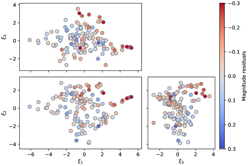
Figure 1: RBTL magnitude residuals as a function of the Twins Embedding coordinates $\xi_{i}$. Each point represents a single SN Ia. The data points are colored according to their RBTL magnitude residuals, as labeled in the colorbar. Each panel shows a different 2D-projection of the Twins Embedding.

The Twins Embedding was designed to capture highly nonlinear features, so there is no reason to expect that the resulting components will be linearly correlated with the peak brightnesses of SNe Ia. Linear standardization as is traditionally done for light curve fitters such as SALT2 is unlikely to be sufficient. Instead, we choose to use Gaussian Process (GP) regression to model the magnitude residuals of SNe Ia over the Twins Embedding. GP regression effectively generates a prediction of the magnitude residuals at a target location in the Twins Embedding using the observed magnitude residuals in a region around that target location. It is also able to propagate uncertainties on the predictions. For an introduction to GP regression, see Appendix A.

When calculating the RBTL magnitude residuals, as described in Section 2.2, we chose to use a fiducial extinction-color relation with $R_{V}=2.8$. If the wrong mean value of $R_{V}$ is chosen, then the only observable effect for this analysis is that a correlation is introduced between the measured extinction and the magnitude residuals. We account for this potential difference in $R_{V}$ by using a mean function in our GP that contains a correction term $\omega$ that is linear in $\Delta\tilde{A}_{V}$ along with an arbitrary reference magnitude $m_{\textrm{ref}}$. For each SN Ia, the magnitude residuals contain uncorrelated measurement uncertainties due to the peculiar velocity of the SN Ia’s host galaxy $\sigma_{\textrm{p.v.},i}$ (described in Section 2.2) and an unexplained residual dispersion $\sigma_{u}$ whose value will be determined in the fit. Measurement uncertainties from the RBTL algorithm are negligible for the high signal-to-noise observations used in this analysis. Any systematic uncertainties from our modeling procedures will be captured by $\sigma_{u}$.

Finally, we use a Matérn 3/2 kernel (see Appendix A) to describe the correlation of the magnitude residuals of SNe Ia across the Twins Embedding. This kernel has two parameters: a length scale $l$ that determines the distances in the Twins Embedding over which the magnitude residuals of different SNe Ia are coherent, and an amplitude $A$ that sets the size of those coherent variations. The Twins Embedding was designed so that the distance between two SNe Ia in the Twins Embedding is proportional to the size of the differences between their spectra. Hence, we choose to use a three-dimensional Matérn kernel with a single length scale. The full GP model is then:

$$\vec{m}_{\textrm{RBTL}}\sim\mathcal{GP}\Bigl{(} m_{\textrm{ref}}+\omega\Delta\vec{\tilde{A}}_{V},$$

$$\mathbf{I}\cdot(\vec{\sigma}_{\textrm{p.v.}}^{2}+\sigma_{u}^{2})+K_{3/2}(\vec{\xi},\vec{\xi};A,l)\Bigl{)}$$ (5)

where $\vec{m}_{\textrm{RBTL}}$ are the RBTL magnitude residuals and $\mathbf{I}$ is the identity matrix.

We implement this GP model using the George package (Ambikasaran et al., 2015). The full model has a total of five parameters: $m_{\textrm{ref}}$, $\omega$, $\sigma_{u}$, $A$, and $l$. We fit this model to the sample of SNe Ia described in Section 2.2 optimizing the maximum likelihood. The results of this fit are shown in Table 4.

Table 4: Parameters for the GP standardization model described in Section 3.3.

Parameter	Value
Extinction $R_{V}$
GP kernel amplitude ($A$)	mag
GP kernel length scale ($l$)
Unexplained dispersion ($\sigma_{u}$)	mag
RMS of $m_{\textrm{corr.},i}$	mag
NMAD of $m_{\textrm{corr.},i}$	mag

Given the fitted extinction correction $\omega$, our estimate of the true extinction-color relation is then the fiducial one with that correction added as a zeropoint offset. We estimate the true value of $R_{V}$ by solving for the extinction-color relation from Fitzpatrick (1999) that best matches this estimated true extinction-color relation. We find that our measurements prefer an $R_{V}$ value of . We verified that different choices of fiducial extinction-color relations result in similar recovered $R_{V}$ values when rerunning the entire analysis. Note that we have rejected SNe Ia with $\Delta\tilde{A}_{V}>0.5$ from this analysis, so our measurement of $R_{V}$ is made using only SNe Ia with relatively low extinction. Previous measurements of $R_{V}$ from optical spectra include $R_{V}=2.8\pm 0.3$ from Chotard et al. (2011) and $R_{V}=2.6\pm 0.5$ from Léget et al. (2020). Mandel et al. (2020) found $R_{V}=2.9\pm 0.2$ from measurements of SNe Ia with infrared photometry. Our results are compatible with, but slightly lower than, these previous measurements of $R_{V}$. The fact that our sample is restricted to low-extinction SNe Ia makes direct comparisons challenging.

The recovered unexplained dispersion of  mag is significantly lower than what is typically found for light curve fitters that only rely on light curve width and color, and is consistent with the results of F15 for pairs of twin supernovae, as will be discussed in Section 4.1. To understand the behavior of the GP, we show the GP predictions after applying the updated $R_{V}$ extinction correction in Figure 2. In these figures, we hold one component value fixed to zero, and show the effects of varying the other two components over the Twins Embedding. Note that these figures only show slices through the GP predictions, and the predictions for individual SNe Ia will also include information from the remaining component that cannot be plotted in only two dimensions. Qualitatively, the GP appears to be able to capture the nonlinear variation in the RBTL magnitude residuals across the Twins Embedding.

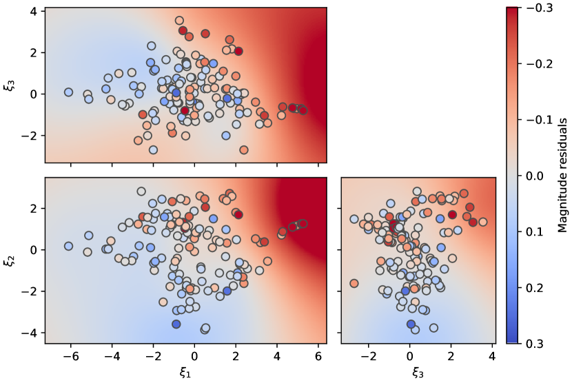
Figure 2: RBTL magnitude residuals and GP predictions as a function of the Twins Embedding coordinates $\xi_{i}$. Each point represents a single SN Ia, colored according to its RBTL magnitude residual. Each panel shows a 2D-projection of the Twins Embedding. The smooth color in the background indicates the amplitude of the GP prediction for each value of the two displayed components while the remaining component is fixed to zero.

We can use the GP to predict what the RBTL magnitude residuals should be for any location in the Twins Embedding, and use these predictions to correct the raw RBTL magnitude residuals. We estimate the magnitude residual of each SN Ia with the GP using individual “leave-one-out” predictions for each SN Ia where the GP is conditioned on all SNe Ia except the supernova of interest. This ensures that the measured brightness of that supernova itself cannot contribute to its own predictions. Using these predictions, we calculate GP-corrected magnitude residuals $m_{\textrm{corr.},i}$ for each SN Ia in our sample as the difference between the raw RBTL magnitude residual and the GP prediction. In Figure 3 we show $m_{\textrm{corr.},i}$ as a function of the location of SNe Ia in the Twins Embedding. In contrast to Figure 1, where we saw strong trends in the raw RBTL magnitude residuals across the twins embedding, there are no visible correlations in $m_{\textrm{corr.},i}$ for SNe Ia that are in similar locations in the Twins Embedding. For the full dataset, we find that the GP-corrected magnitude residuals $m_{\textrm{corr.},i}$ have a dispersion in brightness with an unweighted RMS of  mag and an NMAD of  mag. These dispersions are larger than the unexplained dispersion of  mag because they contain contributions from both peculiar velocities and uncertainties in the GP predictions for SNe Ia in sparsely populated regions of the Twins Embedding.

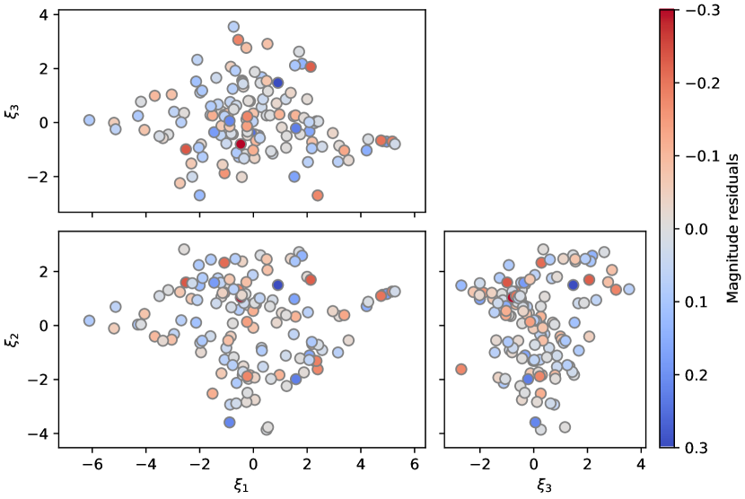
Figure 3: GP-corrected RBTL magnitude residuals $m_{\textrm{corr.},i}$ as a function of the Twins Embedding coordinates $\xi_{i}$. Each point represents a single SN Ia. The data points are colored according to their GP-corrected RBTL magnitude residuals $m_{\textrm{corr.},i}$, as labeled in the colorbar. Each panel shows a different 2D-projection of the Twins Embedding. There is little evidence of correlation between the magnitude residuals of SNe Ia that are nearby in the Twins Embedding, and the remaining observed dispersion is largely driven by peculiar velocity uncertainties.

3.4 Standardizing the SALT2 Magnitude Residuals with the Twins Embedding

We investigate a hybrid standardization method where we use the peak brightness and color from a SALT2 light curve fit, and the Twins Embedding to parametrize the intrinsic variation of SNe Ia instead of the SALT2 $x_{1}$ parameter. While the RBTL method requires that the input spectra be spectrophotometric to obtain accurate estimates of the brightness and extinction of each SN Ia, it may be possible to locate a SN Ia in the Twins Embedding using slit-based spectrographs or other forms of spectroscopy that are not flux-calibrated since most of the information is in local spectral feature variation. External estimates of the brightness and color, from SALT2 fits to photometry for example, could then be corrected using the Twins Embedding.

To test whether this method of standardization might be effective, we ran the GP standardization procedure described in Section 3.3 using the Twins Embedding, but using the raw SALT2 magnitude residuals and colors (uncorrected for $x_{1}$) instead of the RBTL magnitude residuals and extinctions. As for the RBTL analysis, we include a linear term to correct for the SALT2 color, which in this context is equivalent to the $\beta$ parameter in traditional SALT2 analyses. The results of the GP fit for this SALT2 + Twins Embedding model are summarized in Table 5.

Table 5: Parameters for the hybrid SALT2 + Twins Embedding standardization model described in Section 3.4.

Parameter	Value
Color correction ($\beta$)
GP kernel amplitude ($A$)	mag
GP kernel length scale ($l$)
Unexplained dispersion ($\sigma_{u}$)	mag
RMS of $m_{\textrm{corr.},i}$	mag
NMAD of $m_{\textrm{corr.},i}$	mag

As in Section 3.3, we estimate the SALT2 + Twins Embedding GP brightness for each SN Ia using leave-one-out predictions. When raw SALT2 magnitude residuals are standardized using the Twins Embedding, the standardization performance is significantly better than standardizing only on SALT2 $x_{1}$. The resulting unweighted RMS of the SALT2 + Twins Embedding standardized magnitude residuals is  mag compared to  mag for SALT2 with traditional $x_{1}$ standardization for the same set of SNe Ia. Interestingly, the NMAD values of the standardized magnitude residuals are nearly identical for these two analyses ( mag compared to  mag), implying that most of this improvement comes from improving standardization of SNe Ia in the tails of the distribution rather than the core. To illustrate the effect of the Twins Embedding for standardization of raw SALT2 magnitude residuals, we show the GP predictions for the SALT2 + Twins Embedding standardization analysis in Figure 4 along with the color-corrected magnitude residuals for all of the SNe Ia in our sample.

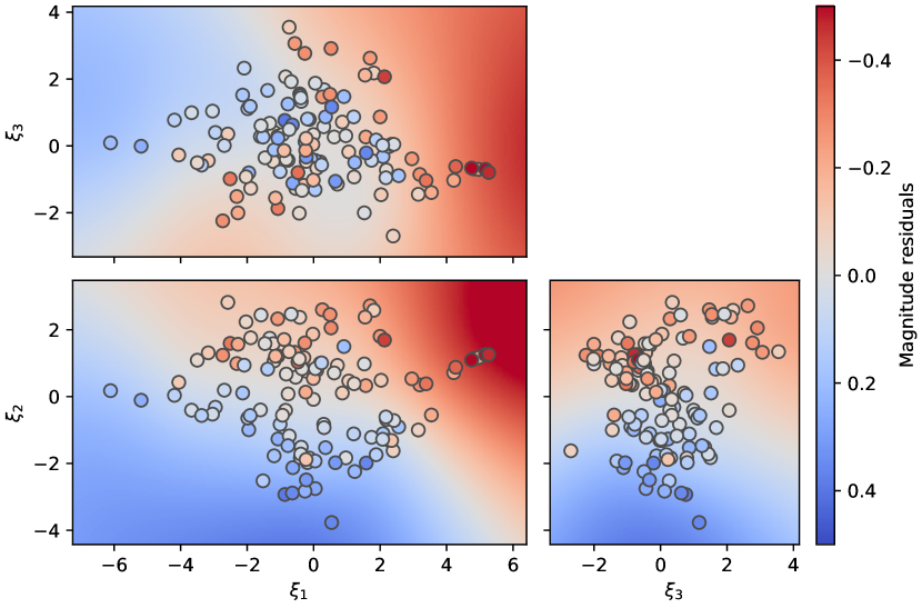
Figure 4: SALT2 magnitude residuals and GP predictions as a function of the Twins Embedding coordinates $\xi_{i}$. Each point represents a single SN Ia, colored according to its SALT2 magnitude residual after applying the color correction. In each panel, the smooth color in the background indicates the amplitude of the GP prediction for each value of the two displayed components while the remaining component is fixed to zero.

For comparison purposes, we show the distribution of the SALT2 $x_{1}$ parameter over the Twins Embedding in Figure 5. Note that $x_{1}$ is highly correlated with $\xi_{2}$, so traditional SALT2 standardization will effectively include a linear correction in $\xi_{2}$. For low values of $x_{1}$, the implied GP magnitude residuals are similar for all SNe Ia with similar values of $x_{1}$. For high values of $x_{1}$, however, the implied GP magnitude residuals vary fairly significantly as a function of the first Twins Embedding component ($\xi_{1}$) in a direction that is orthogonal to the variation in $x_{1}$. This will be discussed in more detail in Section 4.2.

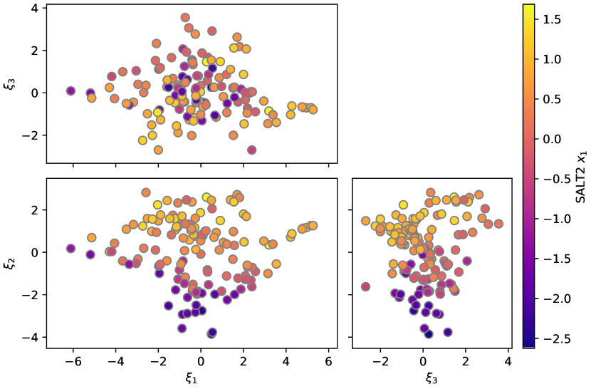
Figure 5: Values of SALT2 $x_{1}$ as a function of the Twins Embedding coordinates $\xi_{i}$. Each data point is a single SN Ia, colored according to its measured SALT2 $x_{1}$ value.

We investigated whether there is any improvement to the Twins Embedding standardization if we include a correction for the SALT2 $x_{1}$ parameter in the model. With a linear correction in SALT2 $x_{1}$, we find that the RMS is improved by only 0.001 mag for the RBTL + Twins Embedding model and 0.004 mag for the SALT2 + Twins Embedding model. This negligible improvement can be explained by the fact that $x_{1}$ is highly correlated with $\xi_{2}$, so including $x_{1}$ in the standardization model does not add any new information.

4 Discussion

4.1 Comparison of Standardization Techniques

In Section 3, we established several different standardization techniques. In this Section, we compare the magnitude residuals from these different techniques. We label the standardization techniques from each section with short names as shown in Table 6.

Table 6: Labels for the different standardization methods described in Section 3

SALT2 + $x_{1}$	Section 3.1
Raw RBTL	Section 3.2
RBTL + Twins Embedding	Section 3.3
SALT2 + Twins Embedding	Section 3.4

We show the measured unweighted RMS and NMAD of the corrected magnitude residuals for all of these techniques in Table 7. These measured RMS values have a contribution from the peculiar velocities of the host galaxies of the SNe Ia, as described in Section 2.2. Assuming a 300 km/s dispersion in velocity, and taking the redshift of each SN Ia in the sample into account, this contributes an added dispersion of  mag to the quoted RMS for the full sample. This dispersion can be removed in quadrature from the quoted values to obtain an estimate of the RMS of magnitude residuals that would be obtained for samples of SNe Ia at higher redshifts where peculiar velocity uncertainties have less of an impact on the magnitude residuals. We also show these “peculiar velocity removed” RMS values in Table 7.

Table 7: Comparison of standardization performance for the different standardization methods and selection requirements. For each method, we show the NMAD, RMS, and unexplained dispersion of the corrected magnitude residuals along with an estimate of the RMS with the peculiar velocity removed (see text for details). Note that with the same sets of cuts, the quoted uncertainties are highly correlated between the different standardization techniques, and therefore do not apply to relative comparisons between different techniques.

Selection	Number of	Statistic	Raw RBTL	RBTL + Twins	SALT2 + $x_{1}$	SALT2 + Twins
Requirements	SNe Ia		Dispersion	Embedding	Dispersion	Embedding
				Dispersion		Dispersion
			(mag)	(mag)	(mag)	(mag)

We find that RBTL + Twins Embedding standardization significantly outperforms both of the SALT2 standardization methods. The variance of the magnitude residuals from the SALT2 + $x_{1}$ standardization is $\sim 2.4$ times that from RBTL + Twins Embedding standardization, meaning that a SN Ia corrected with RBTL + Twins Embedding standardization will have $\sim 2.4$ times the weight in a cosmological analysis compared to a supernova corrected with SALT2 + $x_{1}$ standardization. Note that the quoted uncertainties on the measured RMS do not apply for comparisons between different standardization methods because we are examining the same set of supernovae and most of the residual variation is highly correlated. The RMS for RBTL + Twins Embedding standardization is  mag lower than the RMS for SALT2 + $x_{1}$ standardization, which is an improvement with a significance of $\saltrbtlrmsdiffsig\sigma$.

One somewhat unexpected result is that we find better dispersions for the Raw RBTL magnitude residuals compared to SALT2 + $x_{1}$ corrected magnitudes (RMS of  mag compared to  mag for the set of SNe Ia with valid SALT2 fits). This suggests that even without applying any additional corrections using the intrinsic diversity of the SNe Ia, the base RBTL method standardizes SNe Ia better than does SALT2 with corrections for intrinsic diversity. This was also seen in F15, where even the worst twins had a smaller dispersion in brightness than the SALT2 fits to that same dataset. Some of this difference can be explained by the fact that the RBTL algorithm was constructed to identify the regions of the spectrum of SNe Ia with low intrinsic diversity, and then use these regions of the spectrum to estimate the peak brightness and extinction. Hence its estimate of the peak brightness is less affected by intrinsic diversity than an estimate from the light curve itself. However, we also see that the RBTL + Twins Embedding RMS of  mag is significantly lower than the SALT2 + Twins Embedding RMS of  mag for the same sample of SNe Ia. This suggests that the RBTL algorithm produces estimates of the brightnesses and extinctions of SNe Ia that are more robust than the ones from a light curve fitter like SALT2.

These results can be compared to the analysis of Bailey et al. (2009) who showed that the ratio of fluxes at 6420 Å and 4430 Å can standardize SNe Ia to within $0.125\pm 0.011$ mag. The RBTL algorithm can be thought of as an extension of this procedure where, instead of identifying a single pair of wavelengths where there is low intrinsic diversity, all such wavelengths are used.

4.2 Biases in SALT2 Standardization

We can use the Twins Embedding to look for evidence of biases in SALT2 + $x_{1}$ standardization. We show the SALT2 + $x_{1}$ magnitude residuals as a function of the Twins Embedding components in Figure 6. We see noticeable structure in the residuals, especially for large values of the first and third Twins Embedding components ($\xi_{1}$ and $\xi_{3}$).

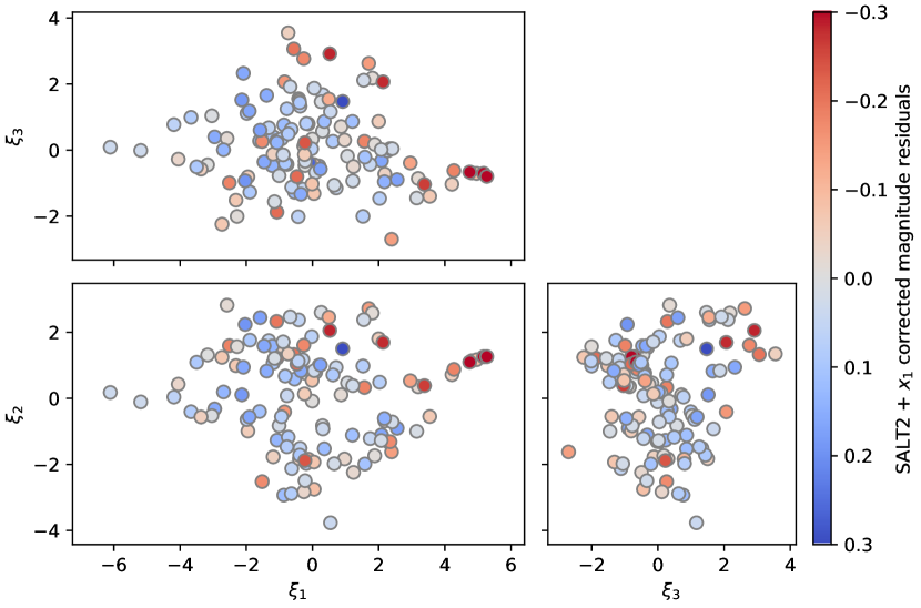
Figure 6: SALT2 + $x_{1}$ corrected magnitude residuals as a function of the Twins Embedding coordinates $\xi_{i}$. We see noticeable structure in the residuals, especially for large values of the first and third Twins Embedding components ($\xi_{1}$ and $\xi_{3}$).

To probe the significance of this result, we examine the SALT2 + $x_{1}$ magnitude residuals with their associated uncertainties as a function of the first Twins Embedding component ($\xi_{1}$) in Figure 7. We label the 91T-like SNe Ia in our sample in this Figure using the labels from Lin et al. (submitted). Extreme values of $\xi_{1}$ correspond to 91T-like SNe Ia. However, we see evidence of a bias even for SNe Ia located at $\xi_{1}$ values between the 91T-like SNe Ia and the rest of the sample. When comparing SNe Ia with $\xi_{1}>3$ to SNe Ia with $\xi_{1}<3$, we find an offset in SALT2 + $x_{1}$ magnitude residuals of  mag. Note that the location of this cut was selected after examining the distribution, which reduces the statistical power of this measurement. However, this strongly suggests that the Twins Embedding is identifying intrinsic diversity of SNe Ia that affects the peak brightness estimates of SNe Ia and that is not captured by measures of the light curve width such as SALT2 $x_{1}$.

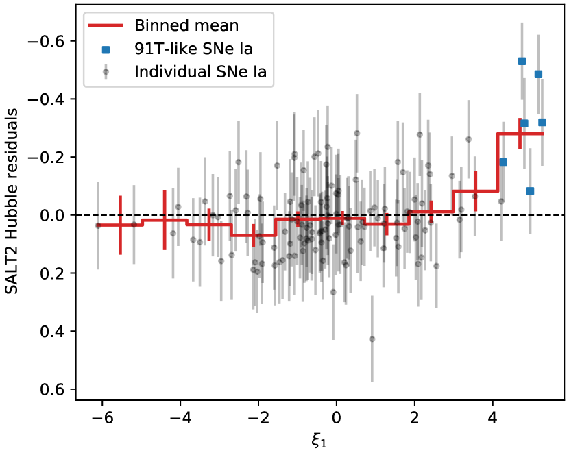
Figure 7: SALT2 + $x_{1}$ corrected magnitude residuals as a function of the first component of the Twins Embedding $\xi_{1}$. The SALT2 magnitude residuals are shown for individual supernovae as gray points with their associated uncertainties. We calculate the mean magnitude residual and its uncertainty in evenly-spaced bins of this component. The results of that procedures are shown with red lines. We find that SALT2 magnitude residuals show a strong bias for large values of $\xi_{1}$. Extreme values of this component are 91T-like SNe Ia, as labeled with blue squares on the plot.

Cosmological analyses using SALT2 for standardization will not be able to identify this subset of SNe Ia as they have normal values of SALT2 $x_{1}$, as shown in Figure 5. This could lead to large systematic biases in cosmological analyses if the relative abundance of this subset changes with redshift. 91T-like SNe Ia are often associated with active star formation (Hakobyan et al., 2020), which increases with redshift. So, for example, if SNe Ia in this subset were twice as abundant at high redshifts compared to low redshifts, then there would be a systematic bias of $\sim$1% in the cosmological distance measurements. This is larger than the projected uncertainties from upcoming surveys with the Vera C. Rubin Observatory (LSST Science Collaboration et al., 2009) or the Nancy Grace Roman Space Telescope (Hounsell et al., 2018). These biases could also exist for surveys that target specific kinds of galaxies, such as Cepheid-hosting galaxies for measurements of the Hubble constant, if the fraction of SNe Ia belonging to the biased subset differs for SNe Ia in these galaxies compared to the overall sample of SNe Ia.

As shown in Article I, there are several other indicators of intrinsic diversity that are highly correlated with $\xi_{1}$ and that could be used to identify this subset of SNe Ia. Notably, Nordin et al. (2018) showed that their “uCa” feature (the flux of a SN Ia in the U-band between 3750 and 3860 Å) can be used to identify 91T-like SNe Ia and improve standardization. The uCa feature is correlated with $\xi_{1}$ and performs a similar role when used for standardization. Other features that could be used to identify these SNe Ia include the pseudo-equivalent width of the Ca II H&K feature, the pseudo-equivalent width of the Si II 6355 Å feature, the second component ($q_{2}$) of the SUGAR model (Léget et al., 2020), or the first component ($c_{1}$) of the SNEMO7 model (Saunders et al., 2018).

These results imply that a SALT2-like model with one component for color and another component for the light curve width is not sufficient to fully capture the intrinsic diversity of SNe Ia relevant to standardization. To emphasize this point, we compare the normal SN Ia  to the 91T-like SN Ia . These two SNe Ia have nearly identical SALT2 parameters, with $x_{1}$ values of  and , and $c$ values of  and  respectively. We show the light curves of these two SNe Ia in the SNfactory bands (defined in Table 1) in Figure 8. The $B_{\mathrm{SNf}}$ and $V_{\mathrm{SNf}}$-band light curves of these two SNe Ia are nearly identical, with differences of less than 0.1 mag for the first 30 days of the light curve. Measurements of the light curve width or other properties in similar bands cannot distinguish between these two SNe Ia. These two SNe Ia do still have significant differences in their light curves: the $U_{\mathrm{SNf}}$, $R_{\mathrm{SNf}}$, and $I_{\mathrm{SNf}}$-band light curves differ by $\sim$0.3 mag before maximum light, and there are differences in the profile of the secondary maximum in the redder bands, which SALT2 does not model and which are not generally measurable for high-redshift SNe Ia.

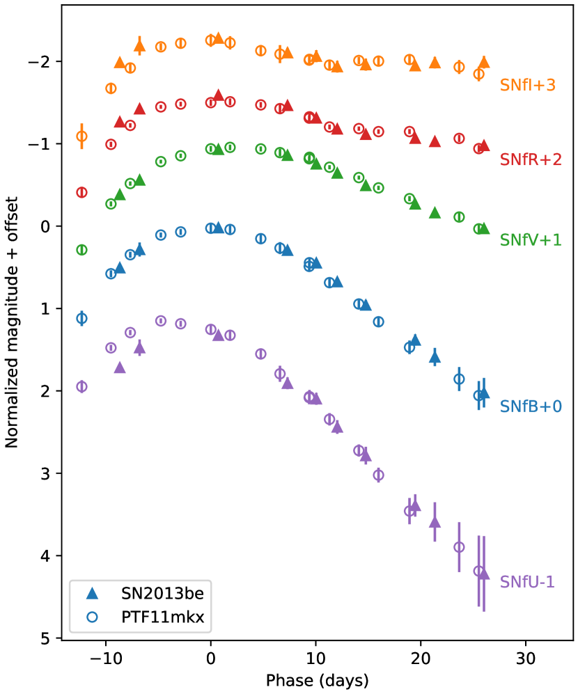
Figure 8: Comparison of the photometry of  and . We show restframe synthetic photometry in the SNfactory bands defined in Table 1. The light curves have been normalized to their individual peak brightnesses in the $B_{\mathrm{SNf}}$ band. The light curves are nearly identical in the $B_{\mathrm{SNf}}$ and $V_{\mathrm{SNf}}$ bands (and best-fit SALT2 parameters), but we see significant differences in the other bands.

The SALT2 fits for the peak $B_{\mathrm{SNf}}$-band luminosities of these two light curves differ by  mag, with the quoted uncertainty including both measurement uncertainties and potential contributions from peculiar velocities. Because they have nearly identical $x_{1}$ and $c$ values, this difference in the luminosities cannot be identified or corrected using SALT2. We show the restframe spectra of these two SNe Ia closest to maximum light in Figure 9. There are large differences in nearly every single spectral feature. This is captured by the Twins Embedding: these two SNe Ia have $\xi_{1}$ values of  and  respectively. With SALT2 + Twins Embedding standardization, as described in Section 3.4, we find a difference between the corrected magnitude residuals of these two SNe Ia of  mag. Hence standardization using the Twins Embedding is able to correctly identify the difference in the luminosities of these two SNe Ia while SALT2-like standardization is not.

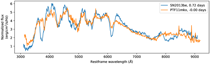
Figure 9: Comparison of the spectra of  and  closest to maximum light. These spectra are shifted to the restframe, scaled so that they have the same brightness in the $B_{\mathrm{SNf}}$ band, and binned to 500 km/s for visual purposes. There are large differences between the spectra in almost all of the spectral features, but they have nearly identical SALT2 $x_{1}$ and $c$ parameters.

4.3 Sufficiency of the Twins Embedding

A similar question is whether the Twins Embedding is sufficient for describing the diversity of spectra at maximum light and whether this impacts standardization. The Twins Embedding was constructed to preserve the spectral distances of F15, and the Euclidean distance between two SNe Ia in the Twins Embedding would be equal to their spectral distance if we kept all of the components of the embedding. We have, however, restricted ourselves to a three component embedding so there could be some SNe Ia that are not well-described by our low-dimensional model.

We show the estimated spectra at maximum light for six different groups of SNe Ia that are nearby in the Twins Embedding in Figure 10. For each of the groups, the spectra of all of the different SNe Ia are remarkably similar with only slight differences around major spectral features. The magnitude residuals for RBTL + Twins Embedding standardization are consistent with zero for each group, in agreement with the discussion in Section 3.3.

We looked for examples of pairs of SNe Ia that were in the worst 50% of F15 spectral distances, but in the best 10% of distances in the Twins Embedding. We found nine such pairings out of the 8,001 pairings considered, all but one of which include SN2007cq. We show the spectrum of SN2007cq and three other nearby SNe Ia that are nearby in the Twins Embedding in Figure 11. The spectrum of SN2007cq shows absorption features near 3600 and 4130 Å that we identify as Ti II that are similar to what is seen in the spectra of 91bg-like SNe Ia. At redder wavelengths, the spectrum of SN2007cq is similar to those of core normal SNe Ia and it does not show the deep Si II and Ca II absorption features that are typical of 91bg-like SNe Ia.

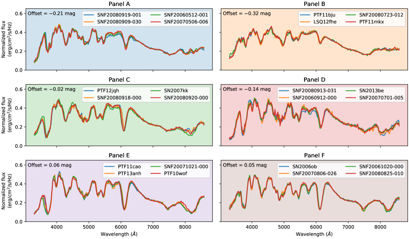
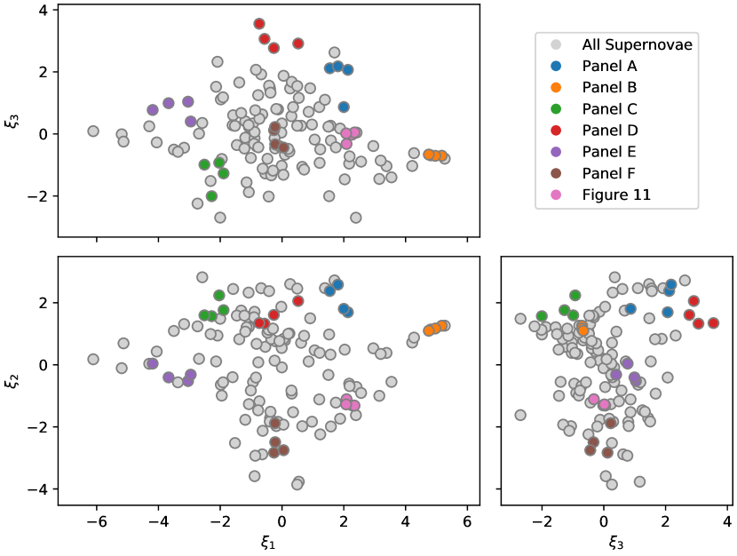
Figure 10: Examples of the spectra of groups of SNe Ia with similar Twins Embedding coordinates. In the bottom plot, we show the locations of each group in different colors. In the top plot we show the estimated spectra at maximum light of four SNe Ia from each group binned to 1000 km/s and with the RBTL brightness and color removed. n the top left corner of each panel, we show the estimated offset in brightness for SNe Ia in each group from RBTL + Twins Embedding standardization. The colors of the panels in the top plot correspond to the markers with the same colors in the bottom plot. We find that the spectra are remarkably similar within each of the groups.

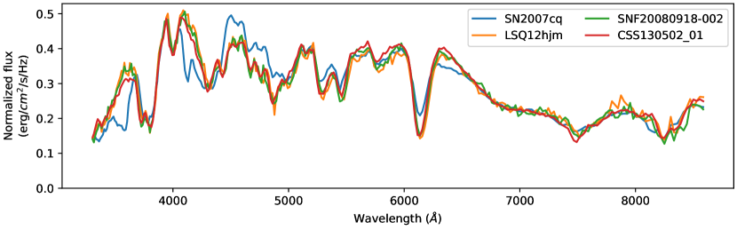
Figure 11: Comparison of the spectra of SNe Ia that are closest to SN2007cq in the Twins Embedding. The spectra are binned to 1000 km/s and the RBTL brightness and color have been removed. These spectra have nearly identical Twins Embedding coordinates and SALT2 $x_{1}$ parameters, but SN2007cq shows absorption features around 3600 and 4130 Å that we identify as Ti II that are not seen in the other spectra. As discussed in the test, SN2007cq is the largest spectral outlier for this analysis, but it has a normal magnitude residual and is not an outlier for RBTL + Twins Embedding standardization.

SN2007cq and its three closest neighbors have very similar SALT2 $x_{1}$ values, between $-0.31$ and $-0.74$, and there are no major differences in their light curves. Despite its unusual spectrum, SN2007cq is not a standardization outlier with RBTL + Twins Embedding standardization: it has an relatively normal magnitude residual of $-0.18\pm 0.12$ mag. The explosions of SNe Ia are very complex, and we expect that there will be some rare SNe Ia whose diversity is not captured by our low dimensional model. SN2007cq is the most egregious such spectral “outlier” in our current analysis, but our standardization methods still perform adequately well for it. We do not find any examples of SNe Ia that have both large magnitude residuals and large spectral differences relative to nearby SNe Ia in the Twins Embedding.

4.4 Correlations with Host Galaxy Properties

As described in Section 1.1, SALT2 standardized magnitude residuals have been shown to have differences of $\sim$0.1 mag when comparing SNe Ia from host galaxies with different properties. We examined how standardization using the Twins Embedding affects these correlations with host galaxy properties. We use the measurements of host galaxy properties from Rigault et al. (2018) (hereafter R18), which includes much of the same set of SNe Ia used in our analysis. The authors of this analysis found that there is a step of $0.163\pm 0.029$ mag when comparing SALT2 residuals from younger environments to older ones, measured using the “local specific star formation rate” (LsSFR). They also found a step of $0.119\pm 0.032$ mag for high-mass hosts compared to low-mass hosts.

We calculated the size of the steps for each of our standardization methods following the same procedure as in R18 as a function of both the host mass and the LsSFR. All SNe Ia are assigned a probability of being on each side of the step given a threshold value and the measurements of the SN Ia host galaxies. We modify the standardization procedures described in Section 3 to simultaneously fit for the size of the host step as part of the standardization procedure. As in R18, we reject peculiar SNe Ia for this analysis, with “peculiar” referring to all SNe Ia that are identified as 91bg-like, 02cx-like or 91T-like in Lin et al. (submitted).

With SALT2 + $x_{1}$ standardization, we find a host step of  mag for LsSFR and  mag for the host mass. These results are consistent with the results found in R18, and differ because we have different selection criteria for our analysis. When standardizing these same SNe Ia using RBTL + Twins Embedding standardization, we find that the host steps are significantly decreased: we find step sizes of  mag for LsSFR and  mag for the host mass.

We also perform several variants on this analysis. First, instead of fitting the step sizes as part of the standardization procedure, we examine the size of them after the standardization correction has already been applied. We do this by fitting a Gaussian mixture model to the corrected magnitude residuals with different means and standard deviations for the magnitude residuals of SNe Ia on either side of the step. We find that the LsSFR step decreases from  mag to  mag between SALT2 + $x_{1}$ standardization and RBTL + Twins Embedding standardization, and the host mass step decreases from  mag to  mag. We show the magnitude residuals and the results of this procedure in Figure 12. Note that the uncertainties in the step measurements are highly correlated. For this analysis variant, we used bootstrap resampling to estimate the significance of the decrease in step size and find that it is significant at the $\hoststepdifflssfrsignificance\sigma$ level for both of the host variables.

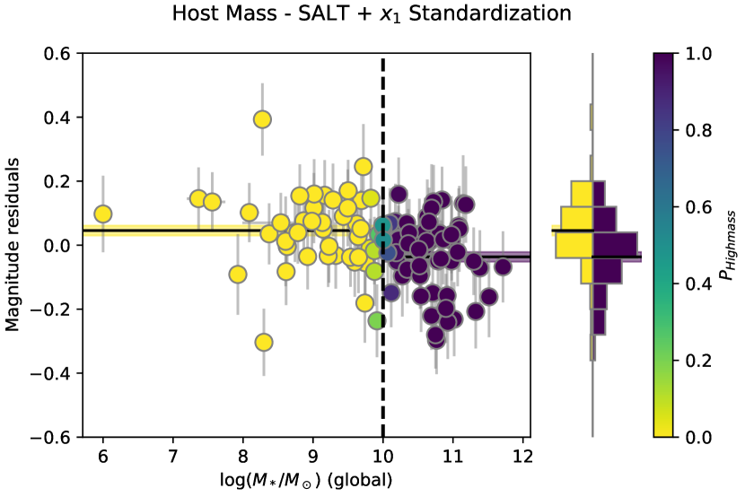
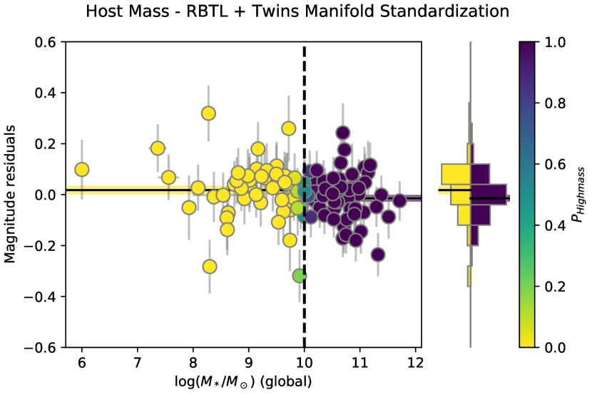
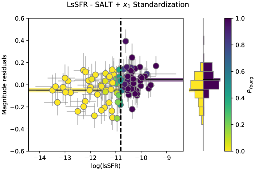
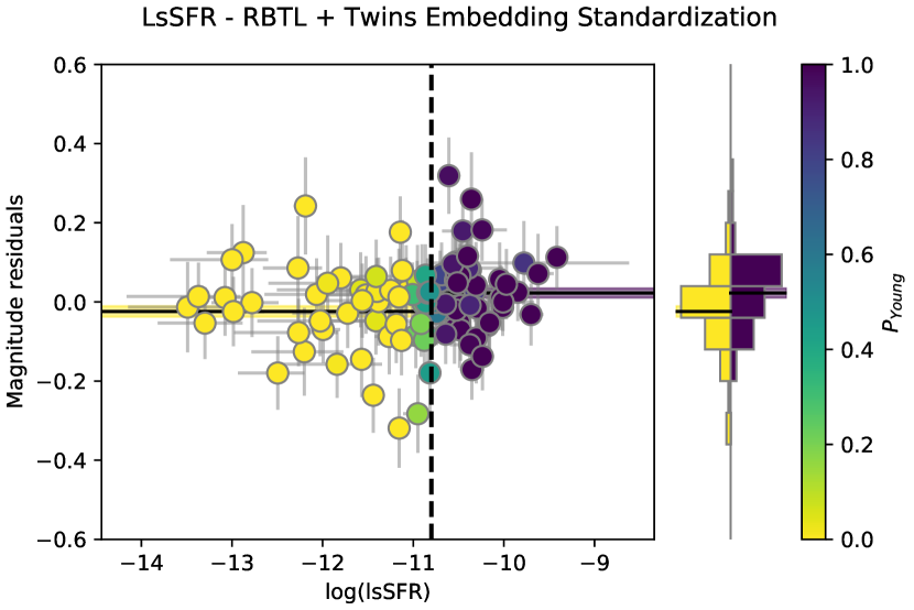
Figure 12: Magnitude residuals as a function of host galaxy properties. The left two panels show SALT2 + $x_{1}$ corrected magnitude residuals while the right two panels show RBTL + Twins Embedding corrected magnitude residuals. The top two panels show the magnitude residuals as a function of the host galaxy mass while the bottom two panels show the magnitude residuals as a function of LsSFR. The marker color represents the probability of each SN Ia being in a low/high mass galaxy or young/old region given the threshold shown as a vertical line. The histograms on the right side of each panel show the distribution of the magnitude residuals for SNe Ia on either side of the threshold. The two horizonal bands show the measured mean magnitude residual for each group and its uncertainty, determined with a Gaussian mixture model as described in the text.

R18 removed all peculiar SNe Ia from their main analysis. We examine how the step sizes are impacted when they are included. Interestingly, the host mass step for SALT2 + $x_{1}$ standardization decreases significantly when we include peculiar SNe Ia from  mag to  mag. The LsSFR step shows a small decrease from  mag to  mag. R18 found similar results. The step sizes for RBTL + Twins Embedding standardization change by less than 0.01 mag. This can be explained by the fact that the SALT2 + $x_{1}$ corrected magnitude residuals of 91T-like peculiar SNe Ia are biased by $\sim$ mag as shown in Section 4.2. For our sample of SNe Ia, the 91T-like SNe Ia are preferentially in low mass/high LsSFR hosts, which artificially decreases the apparent size of the host steps. This result implies that for SALT2 + $x_{1}$ standardization, the size of measured host steps will vary depending on the fraction of 91T-like SNe Ia in the sample. RBTL + Twins Embedding standardization correctly handles 91T-like SNe Ia and is not affected by this.

We measured the step sizes for SALT2 + Twins Embedding standardization, and find very similar results to what is seen for RBTL + Twins Embedding standardzation. The measured host steps for all of these analysis variants are shown in Table 8, and a summary of the host step sizes is shown in Figure 13.

Table 8: Measured host-galaxy property step sizes for different standardization methods. See text for details. We choose to set the sign of the step to be positive for the SALT2 + $x_{1}$ analysis: a negative step means that we recover a step in the opposite direction from the one for the SALT2 + $x_{1}$ analysis.

Analysis variant	Host property	SALT2 + $x_{1}$	RBTL + Twins	SALT2 + Twins
		step size (mag)	Embedding	Embedding
			step size (mag)	step size (mag)

Figure 13: Summary of the host step measurements for the different analysis variants discussed in Section 4.4. For each analysis variant, we show the recovered step sizes for our three different standardization methods in different colors. Note that the uncertainties in the step sizes between different standardization methods are highly correlated: the decrease in host step size is significant at the 3.3–3.7$\sigma$ level for the measurements of host step sizes after correction.

5 Conclusions

In this work, we introduced several methods that can be used to standardize SNe Ia with significantly improved performance compared to traditional SALT2 + $x_{1}$ standardization. With the “Reading Between the Lines” method, we can obtain a robust estimate of the peak brightness and extinction of a SN Ia from a single photometrically-calibrated spectrum at maximum light by using the regions of the spectrum with low intrinsic diversity. We find that the RBTL method on its own is a very good estimator of the distances to SNe Ia, with a dispersion in the RBTL magnitude residuals of  mag. The RBTL algorithm can be applied to all SNe Ia, including ones that are normally labeled as “peculiar”.

We showed that the Twins Embedding introduced in Article I can be used to take into account the intrinsic diversity and standardize the distance estimates from either RBTL or SALT2. Using Gaussian process regression, we estimate the magnitude residual for each SN Ia from its local neighborhood in the Twins Embedding. This significantly improves the standardization of these SNe Ia: we find an RMS dispersion in the corrected magnitude residuals of  mag for conventional SALT2 + $x_{1}$ standardization compared to  mag for SALT2 + Twins Embedding standardization, and  mag for RBTL + Twins Embedding standardization on the same set of SNe Ia.

These dispersions all contain additional scatter due to host galaxy peculiar velocities. For analyses of SNe Ia at higher redshifts or studies of the peculiar velocities themselves, our results imply that RBTL + Twins Embedding standardization is accurate to within  mag compared to  mag for SALT2 + $x_{1}$ standardization. Additionally, a significant fraction of this remaining dispersion is due to uncertainties in the GP model that will be eliminated if this analysis is run using a larger sample of SNe Ia. The remaining unexplained dispersion is  mag for RBTL + Twins Embedding standardization and  mag for SALT2 + Twins Embedding standardization compared to  mag for SALT2 + $x_{1}$ standardization. Note that the uncertainties on all of these RMS dispersion values are correlated: the improved dispersion for RBTL + Twins Embedding standardization relative to SALT2 + $x_{1}$ standardization is significant at the $\saltrbtlrmsdiffsig\sigma$ level.

This decreased dispersion implies that SNe Ia standardized using RBTL + Twins Embedding standardization have $\sim$2.4 times as much weight in a cosmology analysis compared to those standardized using SALT2 + $x_{1}$. This is particularly of interest for studies of nearby SNe Ia, such as measurements of the Hubble constant, where the rate of SNe Ia is limited but high-quality measurements are relatively inexpensive to obtain.

This improved standardization is as important for the systematic uncertainties as it is for the statistical uncertainties, since the systematic uncertainties are constrained to fit within the remaining  mag of unexplained dispersion for the RBTL + Twins Embedding analysis. This is a large improvement over the  mag of unexplained dispersion in the SALT2 + $x_{1}$ analysis. This difference may be in part explained by our finding that SALT2 + $x_{1}$ standardization is biased by  mag for a subset of SNe Ia that can be identified with the first component of the Twins Embedding $\xi_{1}$. This subset of SNe Ia includes, but is not limited to, 91T-like SNe Ia. A major concern for cosmological analyses is that the rates of SNe Ia in different regions of the parameter space could evolve with redshift. If SNe Ia in this region of parameter space have a different rate at high redshifts compared to low redshifts, then they could significantly bias cosmological measurements. With a SALT2 light curve fit, these SNe Ia are indistinguishable from some of the “normal” SNe Ia. However, we showed in this analysis that we can distinguish them from the rest of the sample using the Twins Embedding that was constructed from spectrophotometrically-calibrated spectra at maximum light. Future work needs to be done to determine whether these biased subpopulations can be identified with other techniques such as lower-resolution and lower-signal-to-noise spectroscopy or more advanced light curve fitters.

Upcoming surveys such as the Rubin Observatory’s LSST will not have spectrophotometrically-calibrated spectra near maximum light for the vast majority of the SNe Ia in their sample. This work shows that if these SNe Ia are standardized using traditional light curve fitters such as SALT2, their distance estimates will have intrinsic biases that could affect cosmology results. We are able to use the Twins Embedding to standardize SNe Ia using peak brightnesses and colors estimated from the SALT2 light curve fitter. Targeted spectroscopic follow up campaigns could be used to localize SNe Ia within the Twins Embedding. This could potentially be done without the need for flux-calibrated spectrophotometry, although further studies are necessary to determine how to handle host-galaxy contamination. There is also additional information in the light curve that is not captured by the SALT2 light curve model and that could potentially be used to localize SNe Ia in the Twins Embedding with more advanced light curve models.

Finally, using the Twins Embedding for standardization decreases correlations between distance estimates and the properties of the SN Ia host galaxies. We find that the step in host mass decreases from  mag for SALT2 + $x_{1}$ standardization to  mag for RBTL + Twins Embedding standardization, and the step in LsSFR decreases from  mag to  mag. Both of these decreases are significant at the $\hoststepdifflssfrsignificance\sigma$ level. These results are for a sample where peculiar SNe Ia have already been removed, so the decrease in host step is not due to the SALT2 bias for 91T-like SNe Ia. In fact, we find that including 91T-like SNe Ia in the sample decreases the size of the measured host step, since the 91T-like SNe Ia in our sample have a host step that is in the opposite direction of the one for the rest of the sample. All of these results imply that future surveys need to measure properties of SNe Ia beyond light curve width and color if they are to produce robust cosmological measurements.

The code used to generate all of the results in this analysis is publicly available at https://doi.org/10.5281/zenodo.4670772, and the data are available on the SNfactory website at https://snfactory.lbl.gov/snf/data/.

6 Acknowledgements

We thank the technical staff of the University of Hawaii 2.2-m telescope, and Dan Birchall for observing assistance. We recognize the significant cultural role of Mauna Kea within the indigenous Hawaiian community, and we appreciate the opportunity to conduct observations from this revered site. This work was supported in part by the Director, Office of Science, Office of High Energy Physics of the U.S. Department of Energy under Contract No. DE-AC025CH11231. Additional support was provided by NASA under the Astrophysics Data 1095 Analysis Program grant 15-ADAP15-0256 (PI: Aldering). Support in France was provided by CNRS/IN2P3, CNRS/INSU, and PNC; LPNHE acknowledges support from LABEX ILP, supported by French state funds managed by the ANR within the Investissements d’Avenir programme under reference ANR-11-IDEX-0004-02. Support in Germany was provided by DFG through TRR33 “The Dark Universe” and by DLR through grants FKZ 50OR1503 and FKZ 50OR1602. In China support was provided by Tsinghua University 985 grant and NSFC grant No. 11173017. We thank the Gordon and Betty Moore Foundation for their continuing support. This project has received funding from the European Research Council (ERC) under the European Union’s Horizon 2020 research and innovation programme (grant agreement No. 759194 – USNAC).

Appendix A Gaussian process regression

In this analysis, we use Gaussian process (GP) regression to estimate the magnitude residuals of SNe Ia as a function of their position in the Twins Embedding. A stochastic process $P(x)$ is a GP if for any finite set of points ${x_{1},x_{2},...,x_{n}}$ the distribution ${P(x_{1}),P(x_{2}),...,P(x_{n})}$ is a multivariate normal distribution. A GP can be thought of as a prior over a set of functions. By conditioning the GP on observations, we obtain a posterior containing the set of functions that are consistent with the observations. For a detailed discussion of GPs and their applications, see Rasmussen & Williams (2006).

A GP is uniquely defined by its mean function:

$$\mu(\vec{x})=E[P(\vec{x})]$$ (A1)

and its covariance function, or “kernel”:

$$K(\vec{x}_{1},\vec{x}_{2})=E[(P(\vec{x}_{1})-\mu(\vec{x}_{1}))\times(P(\vec{x}_{2})-\mu(\vec{x_{2}}))]$$ (A2)

We denote this GP using the notation:

$$P(\vec{x})\sim\mathcal{GP}\left(\mu(\vec{x}),K(\vec{x},\vec{x})\right)$$ (A3)

The choice of $\mu$ and $K$ determines how different functions are weighted in the prior of the GP. There are several possible choices for the kernel. For our analyses, we use a Matérn 3/2 kernel:

$$K_{3/2}(\vec{x}_{1},\vec{x}_{2};A,l)=A^{2}\left(1+\sqrt{3\frac{\lVert\vec{x}_{1}-\vec{x}_{2}\rVert^{2}}{l^{2}}}\right)\exp\left(-\sqrt{3\frac{\lVert\vec{x}_{1}-\vec{x}_{2}\rVert^{2}}{l^{2}}}\right)$$ (A4)

The parameter $A$ describes the amplitude scale of the functions that will be produced by the GP, and $l$ sets the length scale over which functions vary. The Twins Embedding is three-dimensional, so each of the points $\vec{x}_{i}$ is also three dimensional. By construction, Euclidean distances in the Twins Embedding directly map to the “spectral distances” between the original spectra. Hence we choose to use a single length scale for all of the dimensions, and simply calculate the distances between any two points in the Twins Embedding using their Euclidean distance, $\lVert\vec{x}_{1}-\vec{x}_{2}\rVert$.

We chose to use a Matérn 3/2 kernel as opposed to the RBF kernel that is commonly used in the literature. The RBF kernel produces infinitely-differentiable functions which can lead to the resulting models being unrealistically smooth (Stein, 1999). In contrast, the Matérn 3/2 kernel produces functions that are only once differentiable which is more realistic for some physical processes. In practice, we find that our results are nearly identical with either kernel.

References

- Aldering et al. (2002) Aldering, G., Adam, G., Antilogus, P., et al. 2002, in Proc. SPIE, Vol. 4836, Survey and Other Telescope Technologies and Discoveries, ed. J. A. Tyson & S. Wolff, 61–72, doi: 10.1117/12.458107
- Aldering et al. (2006) Aldering, G., Antilogus, P., Bailey, S., et al. 2006, ApJ, 650, 510, doi: 10.1086/507020
- Amanullah et al. (2014) Amanullah, R., Goobar, A., Johansson, J., et al. 2014, ApJ, 788, L21, doi: 10.1088/2041-8205/788/2/L21
- Ambikasaran et al. (2015) Ambikasaran, S., Foreman-Mackey, D., Greengard, L., Hogg, D. W., & O’Neil, M. 2015, IEEE Transactions on Pattern Analysis and Machine Intelligence, 38, 252, doi: 10.1109/TPAMI.2015.2448083
- Astier et al. (2006) Astier, P., Guy, J., Regnault, N., et al. 2006, A&A, 447, 31, doi: 10.1051/0004-6361:20054185
- Avelino et al. (2019) Avelino, A., Friedman, A. S., Mandel, K. S., et al. 2019, ApJ, 887, 106, doi: 10.3847/1538-4357/ab2a16
- Bacon et al. (1995) Bacon, R., Adam, G., Baranne, A., et al. 1995, A&AS, 113, 347
- Bacon et al. (2001) Bacon, R., Copin, Y., Monnet, G., et al. 2001, MNRAS, 326, 23, doi: 10.1046/j.1365-8711.2001.04612.x
- Bailey et al. (2009) Bailey, S., Aldering, G., Antilogus, P., et al. 2009, A&A, 500, L17, doi: 10.1051/0004-6361/200911973
- Barone-Nugent et al. (2012) Barone-Nugent, R. L., Lidman, C., Wyithe, J. S. B., et al. 2012, MNRAS, 425, 1007, doi: 10.1111/j.1365-2966.2012.21412.x
- Betoule et al. (2014) Betoule, M., Kessler, R., Guy, J., et al. 2014, A&A, 568, A22, doi: 10.1051/0004-6361/201423413
- Blondin et al. (2011) Blondin, S., Mandel, K. S., & Kirshner, R. P. 2011, A&A, 526, A81, doi: 10.1051/0004-6361/201015792
- Bongard et al. (2011) Bongard, S., Soulez, F., Thiébaut, É., & Pecontal, É. 2011, MNRAS, 418, 258, doi: 10.1111/j.1365-2966.2011.19480.x
- Brout & Scolnic (2020) Brout, D., & Scolnic, D. 2020, arXiv e-prints, arXiv:2004.10206. https://arxiv.org/abs/2004.10206
- Brout et al. (2019) Brout, D., Scolnic, D., Kessler, R., et al. 2019, ApJ, 874, 150, doi: 10.3847/1538-4357/ab08a0
- Burns et al. (2018) Burns, C. R., Parent, E., Phillips, M. M., et al. 2018, ApJ, 869, 56, doi: 10.3847/1538-4357/aae51c
- Buton et al. (2013) Buton, C., Copin, Y., Aldering, G., et al. 2013, A&A, 549, A8, doi: 10.1051/0004-6361/201219834
- Cardelli et al. (1989) Cardelli, J. A., Clayton, G. C., & Mathis, J. S. 1989, ApJ, 345, 245, doi: 10.1086/167900
- Childress et al. (2013) Childress, M., Aldering, G., Antilogus, P., et al. 2013, ApJ, 770, 108, doi: 10.1088/0004-637X/770/2/108
- Chotard et al. (2011) Chotard, N., Gangler, E., Aldering, G., et al. 2011, A&A, 529, L4, doi: 10.1051/0004-6361/201116723
- D’Andrea et al. (2011) D’Andrea, C. B., Gupta, R. R., Sako, M., et al. 2011, ApJ, 743, 172, doi: 10.1088/0004-637X/743/2/172
- Davis et al. (2011) Davis, T. M., Hui, L., Frieman, J. A., et al. 2011, ApJ, 741, 67, doi: 10.1088/0004-637X/741/1/67
- Efron (1979) Efron, B. 1979, Ann. Statist., 7, 1, doi: 10.1214/aos/1176344552
- Fakhouri et al. (2015) Fakhouri, H. K., Boone, K., Aldering, G., et al. 2015, ApJ, 815, 58, doi: 10.1088/0004-637X/815/1/58
- Fitzpatrick (1999) Fitzpatrick, E. L. 1999, PASP, 111, 63, doi: 10.1086/316293
- Foley et al. (2020) Foley, R. J., Hoffmann, S. L., Macri, L. M., et al. 2020, MNRAS, 491, 5991, doi: 10.1093/mnras/stz3324
- Foley et al. (2014) Foley, R. J., Fox, O. D., McCully, C., et al. 2014, MNRAS, 443, 2887, doi: 10.1093/mnras/stu1378
- Gupta et al. (2011) Gupta, R. R., D’Andrea, C. B., Sako, M., et al. 2011, ApJ, 740, 92, doi: 10.1088/0004-637X/740/2/92
- Guy et al. (2007) Guy, J., Astier, P., Baumont, S., et al. 2007, A&A, 466, 11, doi: 10.1051/0004-6361:20066930
- Guy et al. (2010) Guy, J., Sullivan, M., Conley, A., et al. 2010, A&A, 523, A7, doi: 10.1051/0004-6361/201014468
- Hakobyan et al. (2020) Hakobyan, A. A., Barkhudaryan, L. V., Karapetyan, A. G., et al. 2020, MNRAS, 499, 1424, doi: 10.1093/mnras/staa2940
- Hayden et al. (2013) Hayden, B. T., Gupta, R. R., Garnavich, P. M., et al. 2013, ApJ, 764, 191, doi: 10.1088/0004-637X/764/2/191
- Hounsell et al. (2018) Hounsell, R., Scolnic, D., Foley, R. J., et al. 2018, ApJ, 867, 23, doi: 10.3847/1538-4357/aac08b
- Jones et al. (2019) Jones, D. O., Scolnic, D. M., Foley, R. J., et al. 2019, ApJ, 881, 19, doi: 10.3847/1538-4357/ab2bec
- Kasen (2006) Kasen, D. 2006, ApJ, 649, 939, doi: 10.1086/506588
- Kelly et al. (2010) Kelly, P. L., Hicken, M., Burke, D. L., Mandel, K. S., & Kirshner, R. P. 2010, ApJ, 715, 743, doi: 10.1088/0004-637X/715/2/743
- Knop et al. (2003) Knop, R. A., Aldering, G., Amanullah, R., et al. 2003, ApJ, 598, 102, doi: 10.1086/378560
- Kowalski et al. (2008) Kowalski, M., Rubin, D., Aldering, G., et al. 2008, ApJ, 686, 749, doi: 10.1086/589937
- Krisciunas et al. (2004) Krisciunas, K., Suntzeff, N. B., Phillips, M. M., et al. 2004, AJ, 128, 3034, doi: 10.1086/425629
- Lantz et al. (2004) Lantz, B., Aldering, G., Antilogus, P., et al. 2004, in Proc. SPIE, Vol. 5249, Optical Design and Engineering, ed. L. Mazuray, P. J. Rogers, & R. Wartmann, 146–155, doi: 10.1117/12.512493
- Léget et al. (2020) Léget, P. F., Gangler, E., Mondon, F., et al. 2020, A&A, 636, A46, doi: 10.1051/0004-6361/201834954
- Lin et al. (submitted) Lin, Q., Tao, C., Aldering, G., et al. submitted, A&A
- LSST Science Collaboration et al. (2009) LSST Science Collaboration, Abell, P. A., Allison, J., et al. 2009, arXiv e-prints, arXiv:0912.0201. https://arxiv.org/abs/0912.0201
- Mandel et al. (2011) Mandel, K. S., Narayan, G., & Kirshner, R. P. 2011, ApJ, 731, 120, doi: 10.1088/0004-637X/731/2/120
- Mandel et al. (2020) Mandel, K. S., Thorp, S., Narayan, G., Friedman, A. S., & Avelino, A. 2020, arXiv e-prints, arXiv:2008.07538. https://arxiv.org/abs/2008.07538
- Nordin et al. (2018) Nordin, J., Aldering, G., Antilogus, P., et al. 2018, A&A, 614, A71, doi: 10.1051/0004-6361/201732137
- Nugent et al. (1995) Nugent, P., Phillips, M., Baron, E., Branch, D., & Hauschildt, P. 1995, ApJ, 455, L147, doi: 10.1086/309846
- Perlmutter et al. (1999) Perlmutter, S., Aldering, G., Goldhaber, G., et al. 1999, ApJ, 517, 565, doi: 10.1086/307221
- Phillips (1993) Phillips, M. M. 1993, ApJ, 413, L105, doi: 10.1086/186970
- Rasmussen & Williams (2006) Rasmussen, C. E., & Williams, C. K. I. 2006, Gaussian Processes for Machine Learning (MIT Press)
- Riess et al. (2019) Riess, A. G., Casertano, S., Yuan, W., Macri, L. M., & Scolnic, D. 2019, ApJ, 876, 85, doi: 10.3847/1538-4357/ab1422
- Riess et al. (1996) Riess, A. G., Press, W. H., & Kirshner, R. P. 1996, ApJ, 473, 88, doi: 10.1086/178129
- Riess et al. (1998) Riess, A. G., Filippenko, A. V., Challis, P., et al. 1998, AJ, 116, 1009, doi: 10.1086/300499
- Riess et al. (2004) Riess, A. G., Strolger, L.-G., Tonry, J., et al. 2004, ApJ, 607, 665, doi: 10.1086/383612
- Riess et al. (2016) Riess, A. G., Macri, L. M., Hoffmann, S. L., et al. 2016, ApJ, 826, 56, doi: 10.3847/0004-637X/826/1/56
- Rigault et al. (2013) Rigault, M., Copin, Y., Aldering, G., et al. 2013, A&A, 560, A66, doi: 10.1051/0004-6361/201322104
- Rigault et al. (2015) Rigault, M., Aldering, G., Kowalski, M., et al. 2015, ApJ, 802, 20, doi: 10.1088/0004-637X/802/1/20
- Rigault et al. (2018) Rigault, M., Brinnel, V., Aldering, G., et al. 2018, arXiv e-prints. https://arxiv.org/abs/1806.03849
- Roman et al. (2018) Roman, M., Hardin, D., Betoule, M., et al. 2018, A&A, 615, A68, doi: 10.1051/0004-6361/201731425
- Saunders et al. (2018) Saunders, C., Aldering, G., Antilogus, P., et al. 2018, ApJ, 869, 167, doi: 10.3847/1538-4357/aaec7e
- Scalzo et al. (2010) Scalzo, R. A., Aldering, G., Antilogus, P., et al. 2010, ApJ, 713, 1073, doi: 10.1088/0004-637X/713/2/1073
- Schlegel et al. (1998) Schlegel, D. J., Finkbeiner, D. P., & Davis, M. 1998, ApJ, 500, 525, doi: 10.1086/305772
- Scolnic et al. (2018) Scolnic, D. M., Jones, D. O., Rest, A., et al. 2018, ApJ, 859, 101, doi: 10.3847/1538-4357/aab9bb
- Silverman et al. (2012) Silverman, J. M., Ganeshalingam, M., Li, W., & Filippenko, A. V. 2012, MNRAS, 425, 1889, doi: 10.1111/j.1365-2966.2012.21526.x
- Stanishev et al. (2018) Stanishev, V., Goobar, A., Amanullah, R., et al. 2018, A&A, 615, A45, doi: 10.1051/0004-6361/201732357
- Stein (1999) Stein, M. L. 1999, Interpolation of spatial data, Springer Series in Statistics (New York: Springer-Verlag), xviii+247, doi: 10.1007/978-1-4612-1494-6
- Sullivan et al. (2010) Sullivan, M., Conley, A., Howell, D. A., et al. 2010, MNRAS, 406, 782, doi: 10.1111/j.1365-2966.2010.16731.x
- Suzuki et al. (2012) Suzuki, N., Rubin, D., Lidman, C., et al. 2012, ApJ, 746, 85, doi: 10.1088/0004-637X/746/1/85
- Tripp (1998) Tripp, R. 1998, A&A, 331, 815
- Wood-Vasey et al. (2008) Wood-Vasey, W. M., Friedman, A. S., Bloom, J. S., et al. 2008, ApJ, 689, 377, doi: 10.1086/592374