Testing GR with the Gravitational Wave Inspiral Signal GW170817

Abstract

Observations of gravitational waves from compact binary mergers have enabled unique tests of general relativity in the dynamical and non-linear regimes. One of the most important such tests are constraints on the post-Newtonian (PN) corrections to the phase of the gravitational wave signal. The values of these PN coefficients can be calculated within standard general relativity, and these values are different in many alternate theories of gravity. It is clearly of great interest to constrain these deviations based on gravitational wave observations. In the majority of such tests which have been carried out, and which yield by far the most stringent constraints, it is common to vary these PN coefficients individually. While this might in principle be useful for detecting certain deviations from standard general relativity, it is a serious limitation. For example, we would expect alternate theories of gravity to generically have additional parameters. The corrections to the PN coefficients would be expected to depend on these additional non-GR parameters whence, we expect that the various PN coefficients to be highly correlated. We present an alternate analysis here using data from the binary neutron star coalescence GW170817. Our analysis uses an appropriate linear combination of non-GR parameters that represent absolute deviations from the corresponding post-Newtonian inspiral coefficients in the TaylorF2 approximant phase. These combinations represent uncorrelated non-GR parameters which correspond to principal directions of their covariance matrix in the parameter subspace. Our results illustrate good agreement with GR. In particular, the integral non-GR phase is $\Psi_{\mbox{\tiny non-GR}}=(0.447\pm 253)\times 10^{-1}$ and the deviation from GR percentile is $p^{\mbox{\tiny Dev-GR}}_{n}=25.85\%$.

I Introduction

The problem of binary motion in a gravitational system is one of the oldest in astronomy. Newton’s explanation of Kepler’s laws was a milestone of science. Relativistic corrections to Keplerian motion under Newton’s laws have been studied since the time of Einstein Einstein et al. (1938). These corrections can be calculated within the post-Newtonian (PN) formalism as an expansion in the ratio $v/c$ of the typical relative velocity $v$ between the two components of the binary to the speed of light $c$. Low order corrections can be observed in the motion of binary pulsar systems where typical values of $v/c$ are $\mathcal{O}(10^{-4})$ Wex (2014). The recent observations of coalescing compact binary systems (see e.g. Abbott et al. (2016a, 2019a, b); Nitz et al. (2019, 2020); Venumadhav et al. (2020); Zackay et al. (2019)) have much higher values of $v/c\sim\mathcal{O}(10^{-1})$. These observations therefore probe regimes where the gravitational field is strong and also dynamical.

The relation between the binary motion and the observed gravitational waves was first expounded by Peters and Mathews Peters and Mathews (1963). This work obtained the gravitational wave phase by calculating the Einstein quadrupole formula for underlying Keplerian motion. Whilst this analysis gives a very approximate fit for LIGO data Abbott et al. (2017a) it has been known for a long time that more accurate fits require a large number of relativistic corrections Cutler and Flanagan (1994). Several different approaches have been able to model the expected signal for the inspiral and coalescence of compact objects with sufficient accuracy within standard general relativity. These include the Effective-one-body models (see e.g. Buonanno and Damour (1999); Damour and Nagar (2016); Ossokine et al. (2020); Bohé et al. (2017); Taracchini et al. (2014); Pan et al. (2014, 2011); Nagar et al. (2018); Damour and Nagar (2014)), the Phenomenological models (see e.g. Ajith et al. (2008); Khan et al. (2020, 2019); London et al. (2018); Khan et al. (2016); Husa et al. (2016); Santamaria et al. (2010)) and the surrogate models Field et al. (2014); Blackman et al. (2017); Varma et al. (2019). Some corrections have also been calculated in modified gravity theories Ohashi et al. (1996); Nielsen and Birnholtz (2018). In this paper we restrict our attention to the binary neutron star merger GW170817 event Abbott et al. (2017b). For this event, the contribution of the merger to the signal-to-noise-ratio is not significant, whence the inspiral regime and standard PN methods dominate.

It has now become routine to use the observed gravitational wave observations to constrain relativistic corrections to binary motion Arun et al. (2006a, b); Mishra et al. (2010); Abbott et al. (2016c, b, 2019b, 2019c). The TIGER framework Agathos et al. (2014) looks for a deviation from the calculated GR value by introducing a number of phenomenological deviation parameters that take the value zero in GR. In this approach the deviation parameters are assumed to be independent of the physical parameters of the binary, such as mass and spin.

These phenomenological non-GR parameters implicitly represent a certain class of GR alternatives. In different GR alternatives, these parameters may have different physical meanings. For instance, in phenomenological modifications of GR based on the massive graviton assumption, such that the effective Newtonian potential is of Yukawa type with a non-standard graviton dispersion relation, the non-GR parameter of 1PN order is proportional to the graviton’s mass squared Will (1998). In other alternative theories of gravity, radiative multipole moments differ from those of GR and their deviation from GR values contributes to every PN order phase term Kastha et al. (2018, 2019). In general, alternatives to GR may naturally depend on an additional set of parameters such that the non-GR parameters are in general functionally related. This motivates testing GR via the simultaneous variation of such non-GR parameters introduced as additional terms in the GW phase.

In the tests of Abbott et al. (2016b, 2019b, 2019c) two types of variations were considered: each of these parameters was varied individually whilst keeping the others fixed, or all the parameters were varied simultaneously. The results showed that simultaneous variation produced wide and non-informative posteriors on the value of each individual deviation parameter, closely consistent with the prior Abbott et al. (2016c). Whilst varying each one individually captures a generic deviation from GR if it is strong enough, a generic modified gravity theory is expected to differ from GR for several of the non-GR parameters at different PN orders. This also means that one cannot directly compare the results obtained on each parameter individually with a theoretical calculation in an alternate theory of gravity. In addition, the non-GR parameters are correlated with the PN coefficients and between themselves, which can be seen for example in Figure 7 of Abbott et al. (2016c). To remedy these limitations, the method of principal component analysis was proposed in Ohme et al. (2013). A similar method, known as the singular value decomposition approach, was proposed in Pai and Arun (2013). These methods are applied to the Fisher information matrix that estimates parameter values. However, Fisher-matrix-based estimates are not reliable at low SNRs (see, e.g. Cutler and Flanagan (1994) and also Vallisneri (2008)). This limits the measurability of the higher-order PN terms, as well as their non-GR contributions.

In this work, in order to statistically isolate non-GR parameters we diagonalise their covariance matrix derived from the sample data arrays from the PyCBC inference package Biwer et al. (2019). This approach does not rely on the high SNR values that are required for the Fisher information matrix estimate. Using the eigenvectors of the covariance matrix we construct new uncorrelated non-GR parameters (that are linear combinations of the original ones) corresponding to the principal directions of the covariance matrix. In this work, we consider simultaneous variation of non-GR parameters introduced additively to the PN phase expansion parameters from 0PN to 2PN order, although it could be extended to other orders. We demonstrate our method on the signal GW170817 that was identified by the LIGO-Virgo detector network as the first gravitational wave observation of a binary neutron star inspiral Abbott et al. (2017b).

Although, the combined signal-to-noise ratio of 32.4 for GW170817 was the largest of any gravitational wave event observed to date, our primary interest in this system is because of its low mass and long inspiral phase in the detector band. The chirp mass was found to be ${\cal M}=1.188^{+0.004}_{-0.002}\,M_{\odot}$ and with the restriction of the component spins to the range inferred in binary neutron stars, the component masses were found to be in the range $1.17-1.60\,M_{\odot}$, with the total system mass of $2.74^{+0.04}_{-0.01}\,M_{\odot}$. The signal source sky position was localised to an area of 28 deg² with 90$\%$ probability and had a luminosity distance of $40^{+8}_{-14}$ Mpc.

Our paper is organised as follows. In Sec. II we introduce the waveform model and its TaylorF2 approximation up to the 4PN order. We also introduce a set of non-GR additive parameters to the corresponding PN coefficients. All these parameters are given uniform prior distributions and they are varied simultaneously. We derive the corresponding posteriors of all the waveform parameters. Next, diagonalizing of the non-GR parameters covariance matrix, we construct new uncorrelated non-GR parameters and repeat the procedure. In Sec. III we analyse posteriors of the non-GR parameters and define two different methods to measure deviations from GR. We summarise our results in the Conclusion.

II Posterior distributions of the non-GR parameters

When the rate of change of frequency is small relative to the squared frequency, the expansion of a GW signal $h(t)$ in the Fourier domain can be obtained from an expansion in the time domain using the Stationary Phase Approximation Cutler and Flanagan (1994). For the dominant frequency, the Fourier domain waveform can be written as

$$\tilde{h}(f)=A(f)e^{i\Psi(f)}$$ (1)

where $\tilde{h}(f)$ is the Fourier transform of $h(t)$ and

$$\Psi(f) = \sum^{8}_{n=0}\left(\frac{f}{f_{0}}\right)^{(n-5)/3}\left[\Psi_{n}+\Psi^{\ln}_{n}\ln\left(\frac{f}{f_{0}}\right)\right]\,.$$ (2)

Here $\Psi_{1}\equiv 0$ and the only non-zero logarithmic terms are $\Psi^{\ln}_{5}$ and $\Psi^{\ln}_{6}$. The expansion order $n$ corresponds to $(n/2)$PN term. In this expansion the 2.5PN term becomes indistinguishable from the binary coalescence phase $(-\phi_{c}-\pi/4)$ and the 4PN term is indistinguishable from the binary coalescence time $2\pi ft_{c}$. The gravitational wave amplitude $A$ can also be expanded as a post-Newtonian series, but here we will keep only the terms at Newtonian order and hence $A(f)\sim f^{-7/6}$. Factors of a reference frequency $f_{0}$ are included as in Ohme et al. (2013) to render the expansion coefficients explicitly dimensionless. In what follows, we shall take the “natural” reference frequency $f_{\mbox{\tiny ref}}=1/(\pi M)$. This choice matches the expansion (2) of the TaylorF2 approximant form (see, e.g., Buonanno et al. (2009)), which is also implemented in the LALSuite software package LIGO Scientific Collaboration (2018).

The physical parameters that enter our waveform are the binary masses $m_{1}$ and $m_{2}$, the orbit-aligned dimensionless spin components of the stars $\chi_{z1}$ and $\chi_{z2}$ (we consider high-spin priors), the dimensionless deformability parameters $\Lambda_{1}$ and $\Lambda_{2}$, which already appear in the 5PN term (here we present the posterior of the dimensionless combined tidal deformability $\tilde{\Lambda}$), and the following set of non-GR parameters:

$$\delta\Psi_{0}\,,\hskip 7.11317pt\delta\Psi_{1}\,,\hskip 7.11317pt\delta\Psi_{2}\,,\hskip 7.11317pt\delta\Psi_{3}\,,\hskip 7.11317pt\delta\Psi_{4}\,,$$ (3)

that represent the absolute deviations in their corresponding PN coefficients,

$$\Psi_{n}\longrightarrow\Psi_{n}+\delta\Psi_{n}\,.$$ (4)

To obtain the posterior density distributions of these parameters we exploit the PyCBC inference package Biwer et al. (2019). In particular, we use the marginalized phase model and the emcee_pt sampler with 2000 walkers, 12000 effective samples, with a maximum of 1000 samples per chain, and four temperatures. We used (uniform) prior distributions and varied all the parameters simultaneously. One- and two-dimensional posteriors of all the parameters are shown in Fig. 1 and posteriors of the non-GR parameters are shown separately in Fig. 2. One can notice that the dimensionless combined tidal deformability $\tilde{\Lambda}$ is correlated with other parameters, and in particular with $\delta\Psi_{4}$ non-GR parameter.

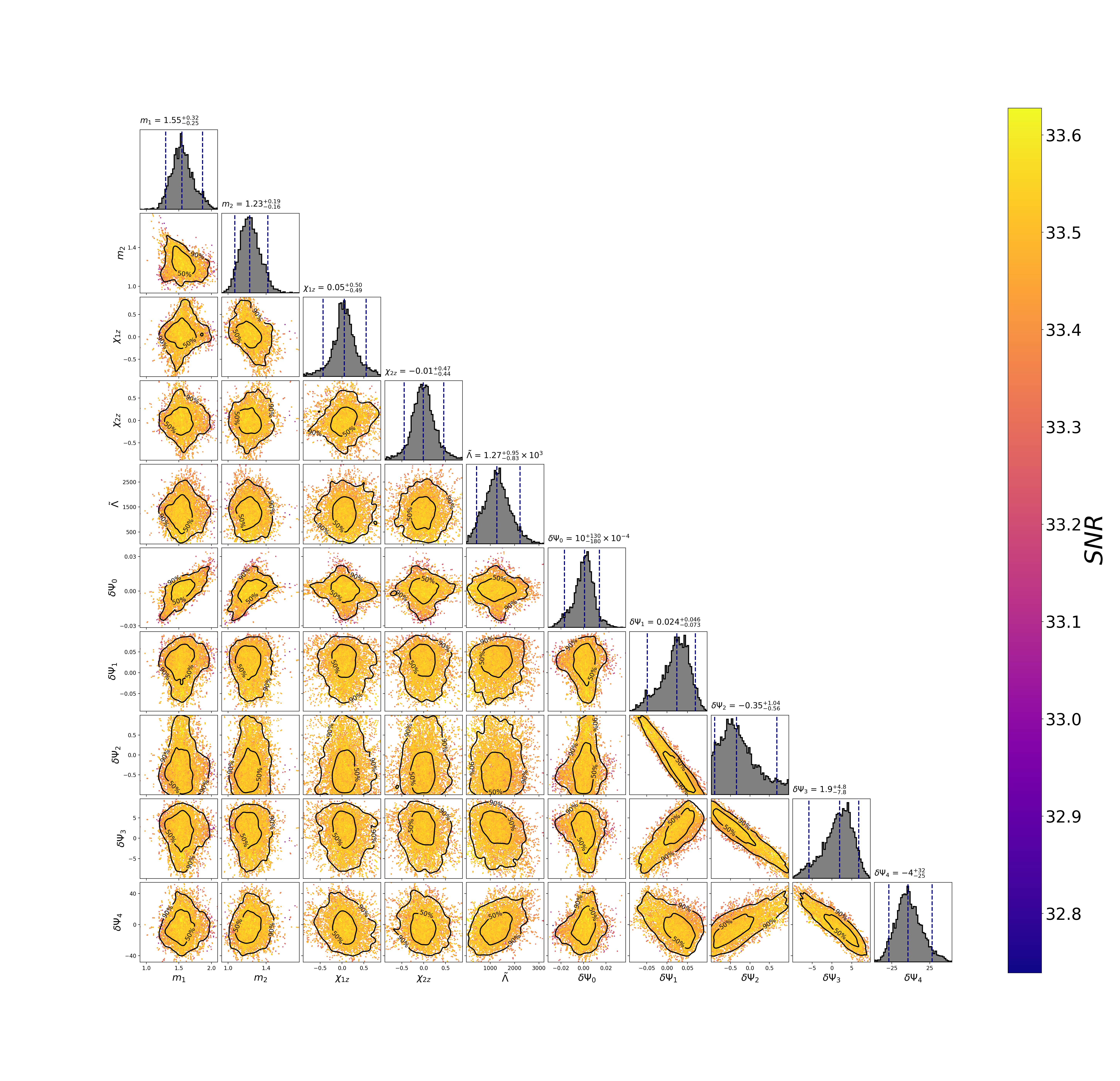
Figure 1: Posterior density distributions of the binary parameters and the non-GR parameters. The central plots are 2D marginal posteriors, where the black contours show the 50% and 90% credible regions. The upper and the right plots are the 1D marginal posteriors, where the median and 90% credible intervals are indicated by the dashed lines.

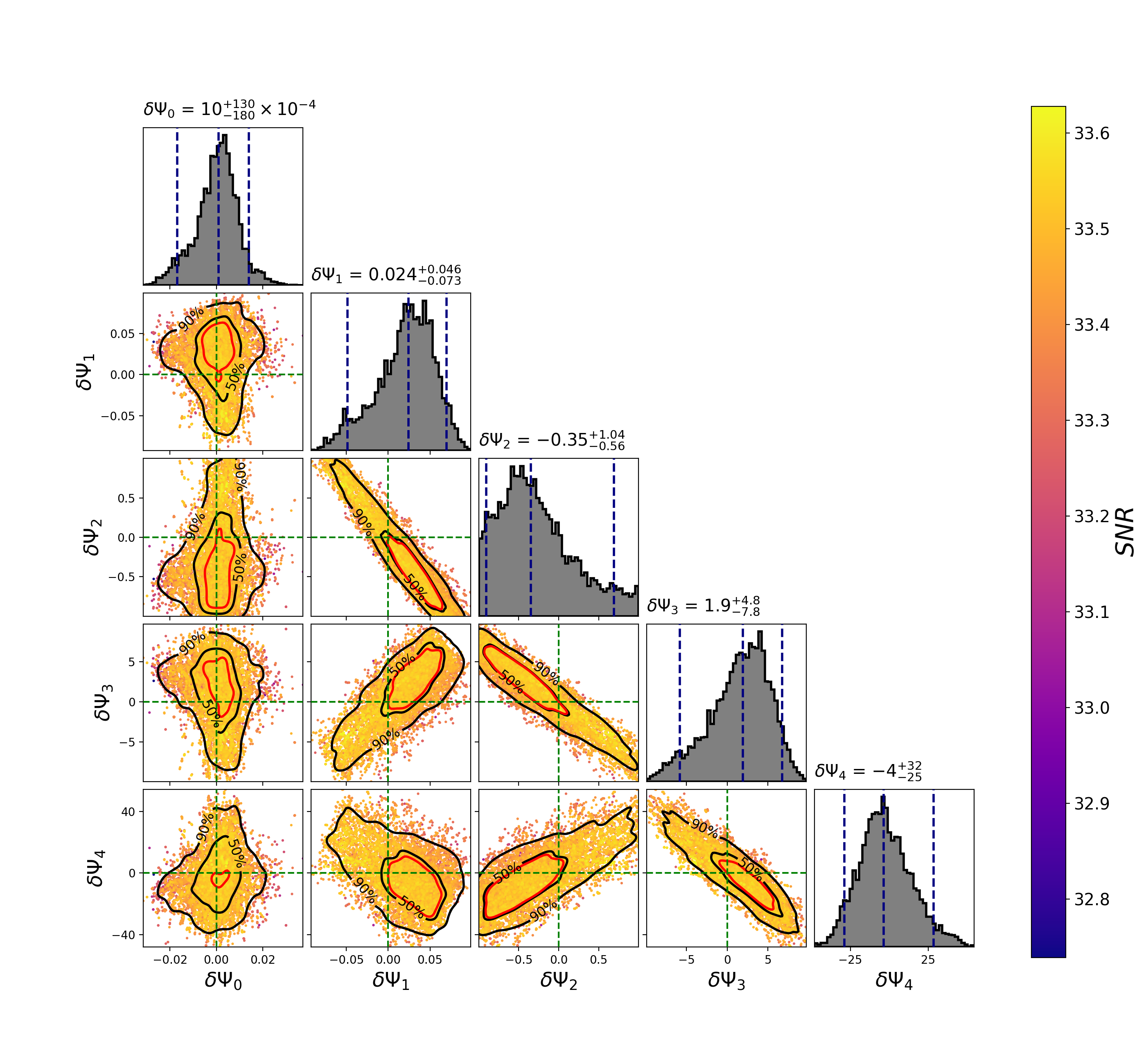
Figure 2: Posterior density distributions of the non-GR parameters from Fig. 1. The central plots are 2D marginal posteriors, where the black contours show the 50% and 90% credible regions. The upper and the right plots are the 1D marginal posteriors, where the median and 90% credible intervals are indicated by the dashed lines. Red contours are defined by vanishing non-GR parameters indicated by intersection of the green dashed lines. They define confidence regions of the 2D joint distributions.

One can infer from Fig. 2 that the non-GR parameters are strongly correlated, in particular $\delta\Psi_{n}$ and $\delta\Psi_{n+1}$, for $n=1,2,3$. The off-diagonal (correlation) terms corresponding to these parameters in the $(5\times 5)$ covariance matrix $\Sigma_{nm}$ make these parameters less accurately measured. Moreover, because of the correlation, we cannot infer directly the accuracy of these parameters from their 1D posteriors. Thus, we are to define a related set of uncorrelated non-GR parameters. To construct such a set we need to diagonalize the covariance matrix $\Sigma_{nm}$. We solve the eigenvalue-eigenvectors problem and derive the transformation matrix $T_{nm}$, which diagonalises the covariance matrix. Its transposed form $T_{mn}$ relates the correlated and new uncorrelated non-GR parameters $\delta\hat{\Psi}_{n}$:

$$\delta\hat{\Psi}_{m}=T_{mn}\delta{\Psi}_{n}\,.$$ (5)

These matrix elements $T_{mn}$ will obviously depend on the detector noise spectrum and on the source parameters as well. Explicitly, the matrix elements which define the transformation are:

$$\left[\begin{array}[]{c}\delta\hat{\Psi}_{0}\\ \delta\hat{\Psi}_{1}\\ \delta\hat{\Psi}_{2}\\ \delta\hat{\Psi}_{3}\\ \delta\hat{\Psi}_{4}\\ \end{array}\right]=\left[\begin{array}[]{ccccc}\,\,\,\,\,3.03\times 10^{-1}&-9.47\times 10^{-1}&-1.08\times 10^{-1}&-4.00\times 10^{-3}&\,\,\,\,\,4.69\times 10^{-4}\\ \,\,\,\,\,9.53\times 10^{-1}&\,\,\,\,\,3.02\times 10^{-1}&\,\,\,\,\,2.98\times 10^{-2}&\,\,\,\,\,5.57\times 10^{-4}&-3.04\times 10^{-4}\\ \,\,\,\,\,4.24\times 10^{-3}&-1.11\times 10^{-1}&\,\,\,\,\,9.80\times 10^{-1}&\,\,\,\,\,1.63\times 10^{-1}&\,\,\,\,\,1.17\times 10^{-2}\\ -1.21\times 10^{-5}&-1.43\times 10^{-2}&\,\,\,\,\,1.61\times 10^{-1}&-9.68\times 10^{-1}&-1.90\times 10^{-1}\\ \,\,\,\,\,9.73\times 10^{-5}&-9.11\times 10^{-4}&\,\,\,\,\,1.97\times 10^{-2}&-1.90\times 10^{-1}&\,\,\,\,\,9.82\times 10^{-1}\\ \end{array}\right]\cdot\left[\begin{array}[]{c}\delta{\Psi}_{0}\\ \delta{\Psi}_{1}\\ \delta{\Psi}_{2}\\ \delta{\Psi}_{3}\\ \delta{\Psi}_{4}\\ \end{array}\right]$$ (6)

The eigenvalue-eigenvectors problem computations were performed using the Householder reduction followed by the QL algorithm. Details of these methods can be found in the book Press et al. (1992).

To illustrate the result of this transformation we present one- and two-dimensional posteriors of the binary parameters together with the uncorrelated non-GR parameters in Fig. 3 and separately the posteriors of the non-GR parameters in Fig. 4.

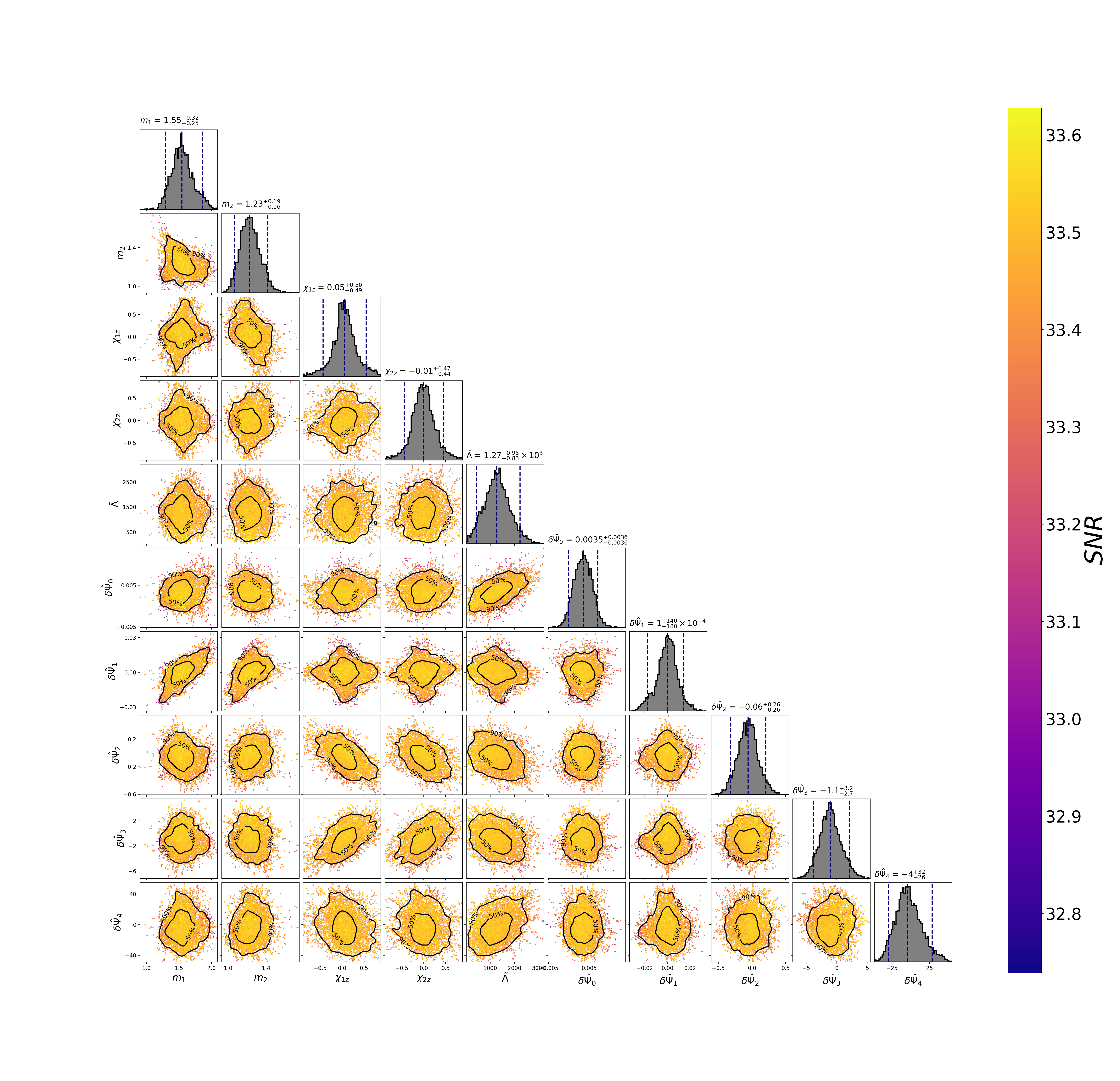
Figure 3: Posterior density distributions of the binary parameters and the uncorrelated non-GR parameters. The central plots are 2D marginal posteriors, where the black contours show the 50% and 90% credible regions. The upper and the right plots are the 1D marginal posteriors, where the median and 90% credible intervals are indicated by the dashed lines.

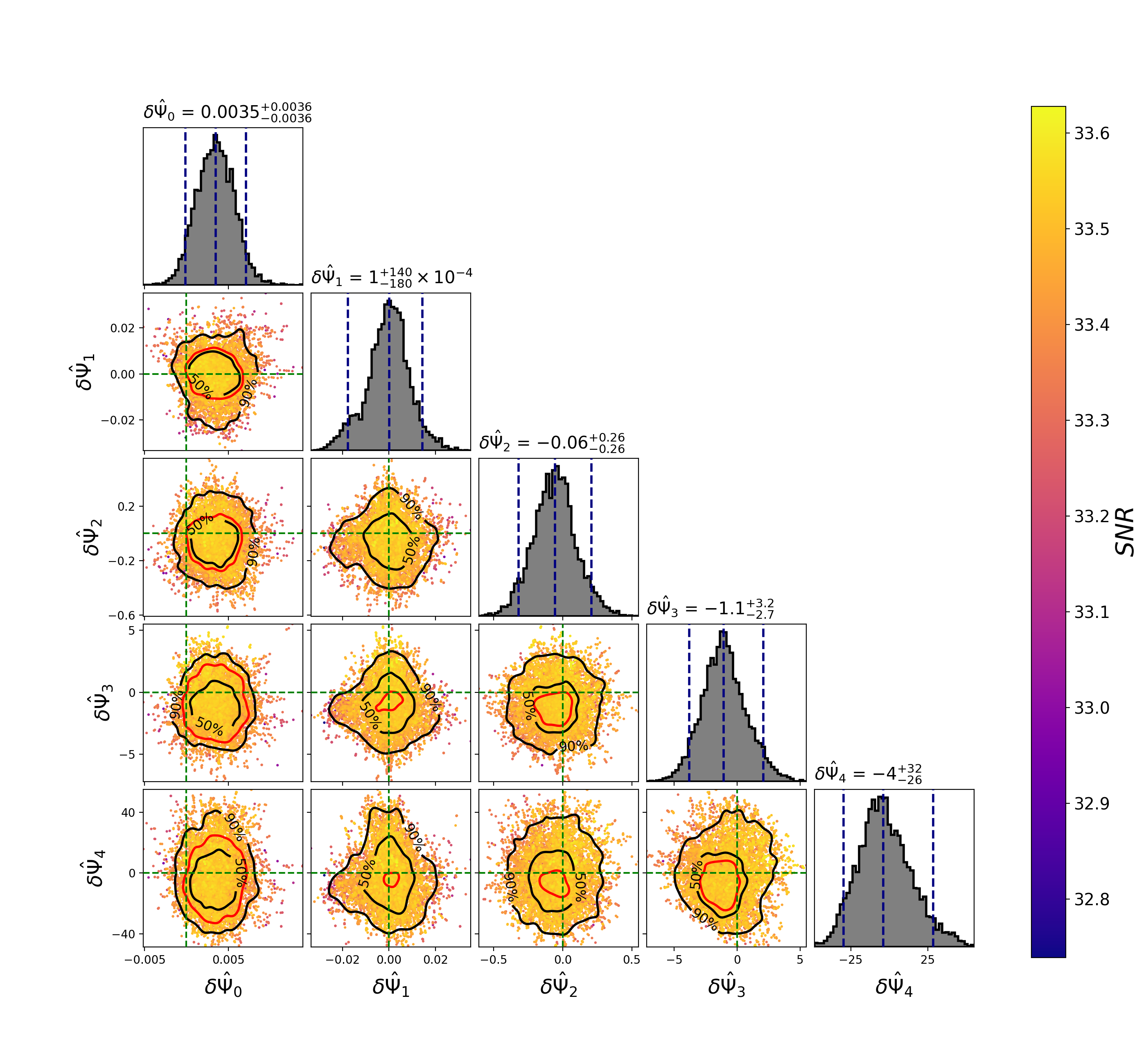
Figure 4: Posterior density distributions of the uncorrelated non-GR parameters. The central plots are 2D marginal posteriors, where the black contours show the 50% and 90% credible regions. The upper and the right plots are the 1D marginal posteriors, where the median and 90% credible intervals are indicated by the dashed lines. Red contours are defined by vanishing non-GR parameters indicated by intersection of the green dashed lines.. They define confidence regions of the 2D joint distributions. For the $\delta\hat{\Psi}_{1}$ and $\delta\hat{\Psi}_{2}$ joint distribution, the GR confidence region is degenerated to the single point $(0,0)$.

One can see that the new non-GR parameters are indeed almost uncorrelated. Moreover, the measured values of the new non-GR parameters are overall more constrained, i.e., more accurate. We note that the presence of the non-GR parameters in the waveform model does affect the values of the physical parameters corresponding to GR waveform model. However, the 90% credible intervals of the “new” values of physical parameters and the “old” ones largely overlap.

III Analysis of the results: Measures of deviations from GR

From the posteriors of the non-GR parameters one can immediately infer that the GR prediction, i.e. $\delta\Psi_{n}=0$, $n=0,...,4$ falls well within their 90% credible intervals. However, one may prefer to have additional quantitative estimates of GR validity. In this section, we measure deviations from GR based on our derived results.

III.1 Integral non-GR phase

According to our approach (2), (4), the waveform phase is an additive combination of the GR and non-GR components,

$$\Psi(f)=\Psi_{\mbox{\tiny GR}}(f)+\Psi_{\mbox{\tiny non-GR}}(f)\,,$$ (7)

where

$$\Psi_{\mbox{\tiny non-GR}}(f)=\sum^{4}_{n=0}\left(\frac{f}{f_{\mbox{\tiny ref}}}\right)^{(n-5)/3}\delta\Psi_{n}\,$$ (8)

is the non-GR part of the waveform phase. In order to measure the non-GR component value we introduce the integral non-GR phase

$$\Psi_{\mbox{\tiny non-GR}}=\int_{f_{\mbox{\tiny min}}/f_{\mbox{\tiny ref}}}^{f_{\mbox{\tiny max}}/f_{\mbox{\tiny ref}}}\Psi_{\mbox{\tiny non-GR}}(f)d\left(f/f_{\mbox{\tiny ref}}\right)\,.$$ (9)

The integral non-GR phase can be computed by using the estimated values of the non-GR parameters [see Fig. 2] and the expression (8) above.

We may also estimate uncertainty $\sigma$ of the non-GR phase by using the propagation of errors approach. The variance of the function (8) is

$$\sigma^{2}(f)=\sum^{4}_{n,m=0}\left(\frac{f}{f_{\mbox{\tiny ref}}}\right)^{(m-5)/3}\Sigma_{nm}\left(\frac{f}{f_{\mbox{\tiny ref}}}\right)^{(n-5)/3}\,.$$ (10)

Integrating this expression in the frequency range, we derive the variance of the non-GR phase

$$\sigma^{2}=\int_{f_{\mbox{\tiny min}}/f_{\mbox{\tiny ref}}}^{f_{\mbox{\tiny max}}/f_{\mbox{\tiny ref}}}\sigma^{2}(f)d\left(f/f_{\mbox{\tiny ref}}\right)\,.$$ (11)

For our data we find

$$\Psi_{\mbox{\tiny non-GR}}=(0.447\pm 253)\times 10^{-1}\,.$$ (12)

Thus, the GR prediction $\Psi_{\mbox{\tiny non-GR}}=0$ falls well within (12).

III.2 Confidence regions and deviation from GR percentile

Here we present another ways to measure GR validity. First, we construct confidence regions whose boundary corresponds to the predicted by GR zero values of the non-GR parameters. This approach is based on the kernel density estimation (kde). For a 2D kde of each pair of the non-GR parameters we used the Python function scipy.stats.gaussian_kde from the SciPy library, that is implemented by PyCBC by the default. The confidence regions are shown in Fig. 2 and Fig. 4.

Second, we calculate the deviation from GR percentile $p^{\mbox{\tiny Dev-GR}}_{n}$ in the following way. The PyCBC inference hdf file contains the posterior for original non-GR PN parameters. We extract the effective samples from the inference hdf file by using pycbc_inference_extract_samples command to get a new hdf file. From this new hdf file, we read the posterior for each original non-GR PN parameters $\delta\Psi_{n}$’s as an array using the standard reading hdf file command. In order to get array for each new non-GR parameter $\delta\hat{\Psi}_{n}$, we use the expression (6). This gives us array for each new non-GR parameter $\delta\hat{\Psi}_{n}$. To get the probability density $p(\delta\hat{\Psi}_{n})$ we use the Python function scipy.stats.gaussian_kde.

The original non-GR PN parameters are correlated, but the new non-GR parameters are almost not correlated. Exploiting this fact, we construct the probability density $P$ in 5 dimensions for the new non-GR parameters by multiplying the individual probability densities $p(\delta\hat{\Psi}_{n})$’s of the new non-GR parameters,

$$P(\delta\hat{\Psi}_{n};n=0,...,4)=\prod_{n=0}^{4}p(\delta\hat{\Psi}_{n})\,.$$ (13)

Next, we define the level hypersurface $\Sigma:\,P=\text{const}$ corresponding to GR prediction, i.e. to zero values of the new non-GR parameters,

$$\Sigma:\,P(\delta\hat{\Psi}_{n};n=0,...,4)=P(\delta\hat{\Psi}_{n}=0;n=0,...,4)\,.$$ (14)

Finally, to get the deviation from GR percentile, we integrate $P$ over the domain $D(\Sigma)$ enclosed by this hypersurface,

$$p^{\text{Dev-GR}}_{n}=\int_{D(\Sigma)}P\,d^{5}(\delta\hat{\Psi}_{n})\,.$$ (15)

To get the value

$$p^{\mbox{\tiny Dev-GR}}_{n}=25.85\%$$ (16)

of the deviation from GR percentile, we performed the integration numerically by using the vegas package, which exploits the adaptive multidimensional Monte Carlo integration.

IV Conclusion

We have analysed deviations from GR with the example of the binary neutron star signal GW170817. A set of 5 non-GR parameters up to and including the 2PN order was introduced into the GW waveform in the TaylorF2 phase approximant. These parameters represent absolute deviations of the post-Newtonian coefficients from their GR values. By using the PyCBC package we computed their posterior density distributions for the simultaneous variation of all these non-GR parameters using uniform prior distributions. Next, diagonalizing their $(5\times 5)$ covariance matrix, we derived linear combinations of these parameters that represent a set of uncorrelated non-GR parameters. This approach allows the first study of each of the new non-GR parameters separately. Each of these uncorrelated parameters corresponds to a covariance matrix principal direction in the 5D subspace of the parameter space.

Our results provide more stringent constraints on GR than those presented in Abbott et al. (2016b, 2019b, 2019c). In comparison to the principal component analysis Ohme et al. (2013) or the singular value decomposition approach Pai and Arun (2013) applied to the Fisher matrix, our computations provide a more efficient technique that achieves more stringent constraints on parameters estimation. Although the approach presented here, based on orthogonalisation of the covariance matrix, looks quite promising, one can also analyse a “hybrid method”, that combines both the principal component analysis of the Fisher matrix and the orthogonalisation of the covariance matrix constructed from the computed data. A more detailed study of this possibility is left for future work.