Goodness of Causal Fit

Abstract

We propose a Goodness of Causal Fit (GCF) measure which depends on Judea Pearl’s “do” interventions. This is different from Goodness of Fit (GF) measures, which do not use interventions. Given a set ${\cal G}$ of DAGs with the same nodes, to find a good $G\in{\cal G}$, we propose plotting $GCF(G)$ versus $GF(G)$ for all $G\in{\cal G}$, and finding a graph $G\in{\cal G}$ with a large amount of both types of goodness.

1 Introduction

Frequently, when students first encounter Bayesian Networks (bnets) and Causal Inference (CI) (Refs.[1], [3]), they experience serious doubts about the usefulness of this theory, because they believe finding the underlying model (i.e., DAG) for most realistic physical situations is too difficult or impossible. I believe that part of the problem is that these students are assuming, perhaps unconsciously, that there exists a unique DAG that fits Nature perfectly, and a mind-boggling number of possibilities to sift through to find that DAG. Rather than looking for a unique DAG, I think a better strategy is to write down a set ${\cal G}$ of likely DAGs, and to calculate for each DAG in ${\cal G}$, a measure called Goodness of Causal Fit (GCF). Then use a DAG with a high GCF score.

The goal of this paper is to propose a GCF measure. Such a measure is of course not unique, and someone may propose in the future a measure that is better than ours.

It’s clear that any measure of GCF will have to involve interventions such as the “do” intervention (see Refs. [1] and [3]) invented by Judea Pearl et al. Without interventions like “do”, it might be impossible to distinguish which DAG of a set is the best causal fit. For example, the family of triangular bnets can all represent the same probability distribution because they are fully connected. Hence, from the probability distribution of the triangular bnet alone, it is impossible to decide which bnet in the family is the best causal fit for the physical situation being considered.

When designing a GCF measure, it is important to keep in mind the Data Axiom of CI: A dataset is causal model-free. In the Data Axiom, when we say a “dataset”, we are referring to a table of data, where all the entries of each column have the same units, and measure a single feature, and each row refers to one particular sample or individual. Datasets are particularly useful for estimating probability distributions and for training neural nets. In the Data Axiom, when we say “causal model”, we are referring to a DAG (directed acyclic graph) or a bnet (bnet= DAG + probability table for each node of DAG).

You can try to derive a causal model from a dataset, but you’ll soon find out that you can only go so far. The process of finding a partial causal model from a dataset is called structure learning (SL). SL can be done quite nicely with Marco Scutari’s open source program bnlearn (Ref[2]). The problem is that SL often cannot narrow down the causal model to a single one. It finds an undirected graph (UG), and it can determine the direction of some of the arrows in the UG, but it is often incapable, for well understood fundamental —not just technical— reasons, of finding the direction of all the arrows of the UG. So it often fails to fully specify a DAG.

Let’s call the ordered pair (dataset, causal model) a dataset++. Then what the Data Axiom is saying is that a dataset is causal model-free or model-less (although sometimes one can find a partial causal model hidden in there). A dataset is not a dataset++.

Graphs which contain both directed and undirected edges are called partially directed (PD) graphs. bnlearn takes a dataset as input and returns a PD graph $G_{pd}$. Given a PD graph $G_{pd}$, let ${\cal G}_{max}(G_{pd})$ be the DAG set which is generated by giving directions to all undirected edges of $G_{pd}$ in all possible ways. We will refer to the DAG set ${\cal G}_{max}(G_{pd})$ as the maximal generation of $G_{pd}$ and to any subset ${\cal G}(G_{pd})$ of ${\cal G}_{max}(G_{pd})$ as a non-maximal generation of $G_{pd}$. Once we define below our GCF measure, we will evaluate it for the DAGs of non-maximal generation ${\cal G}(G_{pg})$.

Henceforth, random variables will be indicated by underlining. Also, Pearl’s do operator assignment $do({\underline{x}})=x$ will be denoted by ${\cal D}{\underline{x}}=x$. Both of these notational conventions are also used in Ref.[3].

2 Goodness of Fit

Before trying to define a GCF measure, it is instructive to review the closely related, well established, measures of Goodness of Fit (GF).

Consider two probability distributions $PO(x)$ and $PE(x)$, where $x\in S_{\underline{x}}$. By a GF measure, we mean a measure of the difference between $PO$ and $PE$. Usually $PO$ is the observed probability distribution and $PE$ is the expected, theoretical one.

Three popular measures of the difference between $PO$ and $PE$ are:

1. The Kullback-Liebler divergence:

   $$D_{KL}(PO\parallel PE)=\sum_{x\in S_{\underline{x}}}PO(x)\ln\frac{PO(x)}{PE(x)}\;.$$ (1)

2. The Pearson divergence (a.k.a. Pearson Chi-squared test statistic):

   $$D_{\chi^{2}}(PO\parallel PE)=\sum_{x\in S_{\underline{x}}}\frac{[PO(x)-PE(x)]^{2}}{PE(x)}=\sum_{x\in S_{\underline{x}}}\frac{PO^{2}(x)}{PE(x)}-1\;.$$ (2)

   It’s easy to show using $\ln(1+\delta)=\delta+{\cal O}(\delta^{2})$ that if $\left|\frac{PO(x)}{PE(x)}-1\right|<<1$ for all $x\in S_{\underline{x}}$, then

   $$D_{KL}(PO\parallel PE)\approx D_{\chi^{2}}(PO\parallel PE)$$ (3)

3. The Euclidean distance squared:

   $$D_{E}(PO,PE)=\sum_{x\in S_{\underline{x}}}[PO(x)-PE(x)]^{2}$$ (4)

Note that of these 3 measures, only $D_{E}(PO,PE)$ is symmetric in $PO$ and $PE$.

Given any bnet $G$ with full probability distribution $P_{G}(x.)$ and a probability distribution $\tilde{P}(x.)$ derived empirically from a dataset, let

$$D(G) = \sum_{x.}\tilde{P}(x.)\ln\frac{\tilde{P}(x.)}{P_{G}(x.)}$$ (5)

$$= D_{KL}(\tilde{P}({\underline{x}}.)\parallel P_{G}({\underline{x}}.))$$ (6)

We define Goodness of Fit (GF) of the bnet $G$ by

$$GF(G)=\ln\frac{1}{D(G)}$$ (7)

3 GCF example 1

$$\begin{array}[]{ccc}\lx@xy@svg{\hbox{\raise 0.0pt\hbox{\kern 5.5pt\hbox{\ignorespaces\ignorespaces\ignorespaces\hbox{\vtop{\kern 0.0pt\offinterlineskip\halign{\entry@#!@&&\entry@@#!@\cr&\\&&\crcr}}}\ignorespaces{\hbox{\kern-3.0pt\raise 0.0pt\hbox{\hbox{\kern 0.0pt\raise 0.0pt\hbox{\hbox{\kern 3.0pt\raise 0.0pt\hbox{$\textstyle{}$}}}}}}}{\hbox{\kern 29.5pt\raise 0.0pt\hbox{\hbox{\kern 0.0pt\raise 0.0pt\hbox{\hbox{\kern 3.0pt\raise 0.0pt\hbox{$\textstyle{{\underline{b}}\ignorespaces\ignorespaces\ignorespaces\ignorespaces\ignorespaces\ignorespaces\ignorespaces\ignorespaces}$}}}}}}}\ignorespaces\ignorespaces\ignorespaces{}\ignorespaces\ignorespaces{{\hbox{\lx@xy@drawline@}}}\ignorespaces{}\ignorespaces\ignorespaces{{\hbox{\lx@xy@drawline@}}}\ignorespaces{{\hbox{\lx@xy@drawline@}}}\ignorespaces\ignorespaces\ignorespaces{}\ignorespaces\ignorespaces{\hbox{\lx@xy@drawline@}}\ignorespaces{\hbox{\kern 64.5pt\raise-30.07571pt\hbox{\hbox{\kern 0.0pt\raise 0.0pt\hbox{\lx@xy@tip{1}\lx@xy@tip{-1}}}}}}\ignorespaces\ignorespaces{\hbox{\lx@xy@drawline@}}\ignorespaces{\hbox{\lx@xy@drawline@}}{\hbox{\kern-5.5pt\raise-35.67776pt\hbox{\hbox{\kern 0.0pt\raise 0.0pt\hbox{\hbox{\kern 3.0pt\raise 0.0pt\hbox{$\textstyle{{\underline{a}}\ignorespaces\ignorespaces\ignorespaces\ignorespaces}$}}}}}}}\ignorespaces\ignorespaces\ignorespaces\ignorespaces{}{\hbox{\lx@xy@droprule}}\ignorespaces{\hbox{\kern 64.5pt\raise-35.67776pt\hbox{\hbox{\kern 0.0pt\raise 0.0pt\hbox{\lx@xy@tip{1}\lx@xy@tip{-1}}}}}}{\hbox{\lx@xy@droprule}}{\hbox{\lx@xy@droprule}}{\hbox{\kern 32.0pt\raise-35.67776pt\hbox{\hbox{\kern 0.0pt\raise 0.0pt\hbox{\hbox{\kern 3.0pt\raise 0.0pt\hbox{$\textstyle{}$}}}}}}}{\hbox{\kern 64.5pt\raise-35.67776pt\hbox{\hbox{\kern 0.0pt\raise 0.0pt\hbox{\hbox{\kern 3.0pt\raise 0.0pt\hbox{$\textstyle{\underline{z}}$}}}}}}}\ignorespaces}}}}\ignorespaces&\lx@xy@svg{\hbox{\raise 0.0pt\hbox{\kern 5.5pt\hbox{\ignorespaces\ignorespaces\ignorespaces\hbox{\vtop{\kern 0.0pt\offinterlineskip\halign{\entry@#!@&&\entry@@#!@\cr&\\&&\crcr}}}\ignorespaces{\hbox{\kern-3.0pt\raise 0.0pt\hbox{\hbox{\kern 0.0pt\raise 0.0pt\hbox{\hbox{\kern 3.0pt\raise 0.0pt\hbox{$\textstyle{}$}}}}}}}{\hbox{\kern 29.5pt\raise 0.0pt\hbox{\hbox{\kern 0.0pt\raise 0.0pt\hbox{\hbox{\kern 3.0pt\raise 0.0pt\hbox{$\textstyle{{\underline{b}}\ignorespaces\ignorespaces\ignorespaces\ignorespaces\ignorespaces\ignorespaces\ignorespaces\ignorespaces}$}}}}}}}\ignorespaces\ignorespaces\ignorespaces{}\ignorespaces\ignorespaces{\hbox{\lx@xy@drawline@}}\ignorespaces{\hbox{\kern 5.50002pt\raise-30.07033pt\hbox{\hbox{\kern 0.0pt\raise 0.0pt\hbox{\lx@xy@tip{1}\lx@xy@tip{-1}}}}}}\ignorespaces\ignorespaces{\hbox{\lx@xy@drawline@}}\ignorespaces{\hbox{\lx@xy@drawline@}}\ignorespaces\ignorespaces\ignorespaces{}\ignorespaces\ignorespaces{\hbox{\lx@xy@drawline@}}\ignorespaces{\hbox{\kern 64.5pt\raise-30.07571pt\hbox{\hbox{\kern 0.0pt\raise 0.0pt\hbox{\lx@xy@tip{1}\lx@xy@tip{-1}}}}}}\ignorespaces\ignorespaces{\hbox{\lx@xy@drawline@}}\ignorespaces{\hbox{\lx@xy@drawline@}}{\hbox{\kern-5.5pt\raise-35.67776pt\hbox{\hbox{\kern 0.0pt\raise 0.0pt\hbox{\hbox{\kern 3.0pt\raise 0.0pt\hbox{$\textstyle{{\underline{a}}\ignorespaces\ignorespaces\ignorespaces\ignorespaces}$}}}}}}}\ignorespaces\ignorespaces\ignorespaces\ignorespaces{}{\hbox{\lx@xy@droprule}}\ignorespaces{\hbox{\kern 64.5pt\raise-35.67776pt\hbox{\hbox{\kern 0.0pt\raise 0.0pt\hbox{\lx@xy@tip{1}\lx@xy@tip{-1}}}}}}{\hbox{\lx@xy@droprule}}{\hbox{\lx@xy@droprule}}{\hbox{\kern 32.0pt\raise-35.67776pt\hbox{\hbox{\kern 0.0pt\raise 0.0pt\hbox{\hbox{\kern 3.0pt\raise 0.0pt\hbox{$\textstyle{}$}}}}}}}{\hbox{\kern 64.5pt\raise-35.67776pt\hbox{\hbox{\kern 0.0pt\raise 0.0pt\hbox{\hbox{\kern 3.0pt\raise 0.0pt\hbox{$\textstyle{\underline{z}}$}}}}}}}\ignorespaces}}}}\ignorespaces&\lx@xy@svg{\hbox{\raise 0.0pt\hbox{\kern 5.5pt\hbox{\ignorespaces\ignorespaces\ignorespaces\hbox{\vtop{\kern 0.0pt\offinterlineskip\halign{\entry@#!@&&\entry@@#!@\cr&\\&&\crcr}}}\ignorespaces{\hbox{\kern-3.0pt\raise 0.0pt\hbox{\hbox{\kern 0.0pt\raise 0.0pt\hbox{\hbox{\kern 3.0pt\raise 0.0pt\hbox{$\textstyle{}$}}}}}}}{\hbox{\kern 29.5pt\raise 0.0pt\hbox{\hbox{\kern 0.0pt\raise 0.0pt\hbox{\hbox{\kern 3.0pt\raise 0.0pt\hbox{$\textstyle{{\underline{b}}\ignorespaces\ignorespaces\ignorespaces\ignorespaces}$}}}}}}}\ignorespaces\ignorespaces\ignorespaces{}\ignorespaces\ignorespaces{\hbox{\lx@xy@drawline@}}\ignorespaces{\hbox{\kern 64.5pt\raise-30.07571pt\hbox{\hbox{\kern 0.0pt\raise 0.0pt\hbox{\lx@xy@tip{1}\lx@xy@tip{-1}}}}}}\ignorespaces\ignorespaces{\hbox{\lx@xy@drawline@}}\ignorespaces{\hbox{\lx@xy@drawline@}}{\hbox{\kern-5.5pt\raise-35.67776pt\hbox{\hbox{\kern 0.0pt\raise 0.0pt\hbox{\hbox{\kern 3.0pt\raise 0.0pt\hbox{$\textstyle{{\underline{a}}\ignorespaces\ignorespaces\ignorespaces\ignorespaces\ignorespaces\ignorespaces\ignorespaces\ignorespaces}$}}}}}}}\ignorespaces\ignorespaces\ignorespaces{}\ignorespaces\ignorespaces{\hbox{\lx@xy@drawline@}}\ignorespaces{\hbox{\kern 32.05566pt\raise-3.0pt\hbox{\hbox{\kern 0.0pt\raise 0.0pt\hbox{\lx@xy@tip{1}\lx@xy@tip{-1}}}}}}\ignorespaces\ignorespaces{\hbox{\lx@xy@drawline@}}\ignorespaces{\hbox{\lx@xy@drawline@}}\ignorespaces\ignorespaces\ignorespaces\ignorespaces{}{\hbox{\lx@xy@droprule}}\ignorespaces{\hbox{\kern 64.5pt\raise-35.67776pt\hbox{\hbox{\kern 0.0pt\raise 0.0pt\hbox{\lx@xy@tip{1}\lx@xy@tip{-1}}}}}}{\hbox{\lx@xy@droprule}}{\hbox{\lx@xy@droprule}}{\hbox{\kern 32.0pt\raise-35.67776pt\hbox{\hbox{\kern 0.0pt\raise 0.0pt\hbox{\hbox{\kern 3.0pt\raise 0.0pt\hbox{$\textstyle{}$}}}}}}}{\hbox{\kern 64.5pt\raise-35.67776pt\hbox{\hbox{\kern 0.0pt\raise 0.0pt\hbox{\hbox{\kern 3.0pt\raise 0.0pt\hbox{$\textstyle{\underline{z}}$}}}}}}}\ignorespaces}}}}\ignorespaces\\ G_{pd}&G_{1}&G_{2}\end{array} \textstyle{{\underline{b}}\ignorespaces\ignorespaces\ignorespaces\ignorespaces\ignorespaces\ignorespaces\ignorespaces\ignorespaces} \textstyle{{\underline{a}}\ignorespaces\ignorespaces\ignorespaces\ignorespaces} \textstyle{\underline{z}} \textstyle{{\underline{b}}\ignorespaces\ignorespaces\ignorespaces\ignorespaces\ignorespaces\ignorespaces\ignorespaces\ignorespaces} \textstyle{{\underline{a}}\ignorespaces\ignorespaces\ignorespaces\ignorespaces} \textstyle{\underline{z}} \textstyle{{\underline{b}}\ignorespaces\ignorespaces\ignorespaces\ignorespaces} \textstyle{{\underline{a}}\ignorespaces\ignorespaces\ignorespaces\ignorespaces\ignorespaces\ignorespaces\ignorespaces\ignorespaces} \textstyle{\underline{z}} \textstyle{{\underline{b}}\ignorespaces\ignorespaces\ignorespaces\ignorespaces\ignorespaces\ignorespaces\ignorespaces\ignorespaces} \textstyle{{\underline{a}}\ignorespaces\ignorespaces\ignorespaces\ignorespaces} \textstyle{\underline{z}} \textstyle{{\underline{b}}\ignorespaces\ignorespaces\ignorespaces\ignorespaces\ignorespaces\ignorespaces\ignorespaces\ignorespaces} \textstyle{{\underline{a}}\ignorespaces\ignorespaces\ignorespaces\ignorespaces} \textstyle{\underline{z}} \textstyle{{\underline{b}}\ignorespaces\ignorespaces\ignorespaces\ignorespaces} \textstyle{{\underline{a}}\ignorespaces\ignorespaces\ignorespaces\ignorespaces\ignorespaces\ignorespaces\ignorespaces\ignorespaces} \textstyle{\underline{z}}$$

Figure 1: ${\cal G}(G_{pd})=\{G_{1},G_{2}\}$. From the partially directed graph $G_{pd}$, one can generate the DAGs $G_{1}$ and $G_{2}$ by giving directions to all undirected edges of $G_{pd}$ in all possible ways. (In this case, there is only one undirected edge in $G_{pd}$.)

For the first example of our GCF measure, we consider ${\cal G}(G_{pd})=\{G_{1},G_{2}\}$ given by Fig.1. We will assume the following:

• First, we assume that we have collected a dataset from which we have extracted a full empirical distribution $\tilde{P}(z,a,b)$. From $\tilde{P}(z,a,b)$, we assume that the following have been calculated. $\tilde{P}(a)$, $\tilde{P}(b)$.

• Second, we assume that a dataset has been collected for which ${\underline{a}}$ was held fixed to each of the possible values $a\in S_{\underline{a}}$ of ${\underline{a}}$. Furthermore, we assume that the distribution $\tilde{P}(b|{\cal D}{\underline{a}}=a)$ has been calculated from that dataset.

• Third, we assume that a dataset has been collected for which ${\underline{b}}$ was held fixed to each of the possible values $b\in S_{\underline{b}}$ of ${\underline{b}}$. Furthermore, we assume that the distribution $\tilde{P}(a|{\cal D}{\underline{b}}=b)$ has been calculated from that dataset.

We will refer to $\tilde{P}(b|{\cal D}{\underline{a}}=a)$ and $\tilde{P}(a|{\cal D}{\underline{b}}=b)$ as empirical do-probability distributions.

Now define

$${\cal H}_{a}^{{\underline{a}}\text{---}{\underline{b}}} = \sum_{b}\tilde{P}(b)\ln\frac{\tilde{P}(b)}{\tilde{P}(b|{\cal D}{\underline{a}}=a)}$$ (8)

$$= D_{KL}(\tilde{P}({\underline{b}})\parallel\tilde{P}({\underline{b}}|{\cal D}{\underline{a}}=a))$$ (9)

$${\cal H}_{\underline{a}}^{{\underline{a}}\text{---}{\underline{b}}} = \sum_{a}\tilde{P}(a){\cal H}_{a}^{{\underline{a}}\text{---}{\underline{b}}}$$ (10)

$$= E_{a}[{\cal H}_{a}^{{\underline{a}}\text{---}{\underline{b}}}]$$ (11)

and

$${\cal H}_{b}^{{\underline{a}}\text{---}{\underline{b}}} = D_{KL}(\tilde{P}({\underline{a}})\parallel\tilde{P}({\underline{a}}|{\cal D}{\underline{b}}=b))$$ (12)

$${\cal H}_{\underline{b}}^{{\underline{a}}\text{---}{\underline{b}}} = \sum_{a}\tilde{P}(b){\cal H}_{b}^{{\underline{a}}\text{---}{\underline{b}}}$$ (13)

$$= E_{b}[{\cal H}_{b}^{{\underline{a}}\text{---}{\underline{b}}}]\;.$$ (14)

We will refer to ${\cal H}_{\underline{x}}$ for any node ${\underline{x}}$ as the hospitality of node ${\underline{x}}$. Note that the hospitality for node ${\underline{x}}$ is zero if node ${\underline{x}}$ has no incoming arrows (i.e., is “inhospitable”), and becomes positive if node ${\underline{x}}$ does have some incoming arrows (i.e., is “hospitable”).

Note that if the truth is $G_{2}$ with ${\underline{a}}\rightarrow{\underline{b}}$, then

$${\cal H}_{a}^{{\underline{a}}\text{---}{\underline{b}}}=0\text{ for all $a$ so }\underbrace{{\cal H}_{\underline{a}}^{{\underline{a}}\text{---}{\underline{b}}}}_{0}\leq{\cal H}_{\underline{b}}^{{\underline{a}}\text{---}{\underline{b}}}$$ (15)

and if the truth is $G_{1}$ with ${\underline{b}}\rightarrow{\underline{a}}$, then

$${\cal H}_{b}^{{\underline{a}}\text{---}{\underline{b}}}=0\text{ for all $b$ so }{\cal H}_{\underline{a}}^{{\underline{a}}\text{---}{\underline{b}}}\geq\underbrace{{\cal H}_{\underline{b}}^{{\underline{a}}\text{---}{\underline{b}}}}_{0}\;.$$ (16)

Hence, no matter what the truth is, the arrow connecting nodes ${\underline{a}}$ and ${\underline{b}}$ always points towards the larger of the 2 hospitalities (i.e., the arrow “seeks the most hospitable node”)

If ${\cal H}_{\underline{a}}^{{\underline{a}}\text{---}{\underline{b}}}\leq{\cal H}_{\underline{b}}^{{\underline{a}}\text{---}{\underline{b}}}$, then define $GCF(G_{1})=-1$ and $GCF(G_{2})=+1$.

If ${\cal H}_{\underline{b}}^{{\underline{a}}\text{---}{\underline{b}}}\leq{\cal H}_{\underline{a}}^{{\underline{a}}\text{---}{\underline{b}}}$, then define $GCF(G_{1})=+1$ and $GCF(G_{2})=-1$.

4 GCF example 2

               

Figure 2: ${\cal G}=\{G_{1},G_{2},G_{3}\}$. ${\cal G}$ is a set of observationally equivalent (OE) graphs. These are graphs that have the same full probability distribution, and are therefore indistinguishable by means of GF alone. For more info about OE graphs, see Chapter entitled “Observationally Equivalent DAGs” in Ref.[3]. Note that ${\cal G}_{max}(G_{pd})$ includes one more DAG, the one in which node ${\underline{x}}_{1}$ is a collider. Hence ${\cal G}$ is a non-maximal generation of $G_{pd}$.

For the second example of our GCF measure, consider ${\cal G}=\{G_{1},G_{2},G_{3}\}$ given by Fig.2.

The relative size of the hospitalities ${\cal H}_{{\underline{x}}_{2}}^{{\underline{x}}_{2}\text{---}{\underline{x}}_{1}}$, ${\cal H}_{{\underline{x}}_{1}}^{{\underline{x}}_{2}\text{---}{\underline{x}}_{1}}$, ${\cal H}_{{\underline{x}}_{1}}^{{\underline{x}}_{1}\text{---}{\underline{x}}_{3}}$ and ${\cal H}_{{\underline{x}}_{3}}^{{\underline{x}}_{1}\text{---}{\underline{x}}_{3}}$, depends on the empirical do-probability distributions. For definiteness, suppose the sizes of these hospitalities are related as follows:

$${\cal H}_{{\underline{x}}_{2}}^{{\underline{x}}_{2}\text{---}{\underline{x}}_{1}}\leq{\cal H}_{{\underline{x}}_{1}}^{{\underline{x}}_{2}\text{---}{\underline{x}}_{1}},\quad\quad{\cal H}_{{\underline{x}}_{1}}^{{\underline{x}}_{1}\text{---}{\underline{x}}_{3}}\leq{\cal H}_{{\underline{x}}_{3}}^{{\underline{x}}_{1}\text{---}{\underline{x}}_{3}}\;.$$ (17)

For any two hospitalities ${\cal H}_{\underline{a}}^{{\underline{a}}\text{---}{\underline{b}}}$ and ${\cal H}_{\underline{b}}^{{\underline{a}}\text{---}{\underline{b}}}$, let

$$d_{{\underline{b}},{\underline{a}}}=|{\cal H}_{\underline{b}}^{{\underline{a}}\text{---}{\underline{b}}}-{\cal H}_{\underline{a}}^{{\underline{a}}\text{---}{\underline{b}}}|$$ (18)

If we abbreviate ${\underline{x}}_{j}$ by $j$, we can define the GCF for each of the graphs in ${\cal G}$ by:

$$GCF(G_{1})=\frac{-d_{2,1}+d_{1,3}}{d_{2,1}+d_{1,3}}$$ (19a)

$$GCF(G_{2})=\frac{d_{2,1}+d_{1,3}}{d_{2,1}+d_{1,3}}=1$$ (19b)

$$GCF(G_{3})=\frac{-d_{2,1}-d_{1,3}}{d_{2,1}+d_{1,3}}=-1$$ (19c)

5 GCF in general

Suppose $G_{i}\in{\cal G}$, where ${\cal G}$ is a non-maximal generation of $G_{pd}$. In that case, we define a GCF measure as follows. Note that the following definition generalizes the definition of GCF measure that was used in the 2 special cases that we have considered so far.

For any bnet $G_{i}\in{\cal G}$ with nodes ${\underline{a}}$ and ${\underline{b}}$, define the hospitality of node ${\underline{b}}$ by

$${\cal H}_{b}^{{\underline{a}}\text{---}{\underline{b}}} = D_{KL}(\tilde{P}({\underline{a}})\parallel\tilde{P}({\underline{a}}|{\cal D}{\underline{b}}=b))$$ (20)

$${\cal H}_{\underline{b}}^{{\underline{a}}\text{---}{\underline{b}}} = \sum_{a}\tilde{P}(b){\cal H}_{b}^{{\underline{a}}\text{---}{\underline{b}}}$$ (21)

$$= E_{b}[{\cal H}_{b}^{{\underline{a}}\text{---}{\underline{b}}}]\;.$$ (22)

For any two hospitalities ${\cal H}_{\underline{a}}^{{\underline{a}}\text{---}{\underline{b}}}$ and ${\cal H}_{\underline{b}}^{{\underline{a}}\text{---}{\underline{b}}}$, define the hospitality distance by

$$d_{{\underline{b}},{\underline{a}}}=|{\cal H}_{\underline{b}}^{{\underline{a}}\text{---}{\underline{b}}}-{\cal H}_{\underline{a}}^{{\underline{a}}\text{---}{\underline{b}}}|$$ (23)

Note that $d_{{\underline{b}},{\underline{a}}}=0$ iff ${\cal H}_{\underline{a}}^{{\underline{a}}\text{---}{\underline{b}}}={\cal H}_{\underline{b}}^{{\underline{a}}\text{---}{\underline{b}}}$. See Appendix A for a proof that if ${\cal H}_{\underline{a}}^{{\underline{a}}\text{---}{\underline{b}}}={\cal H}_{\underline{b}}^{{\underline{a}}\text{---}{\underline{b}}}$, then there is no arrow between ${\underline{a}}$ and ${\underline{b}}$.

For any $G_{i}\in{\cal G}$, define the edge reward function by

$$\rho_{G_{i}}({\underline{a}}\text{---}{\underline{b}})=\left\{\begin{array}[]{ll}+1&\text{ if edge ${\underline{a}}\text{---}{\underline{b}}$ in $G_{i}$ points towards the larger of ${\cal H}_{\underline{a}}^{{\underline{a}}\text{---}{\underline{b}}}$ and ${\cal H}_{\underline{b}}^{{\underline{a}}\text{---}{\underline{b}}}$.}\\ -1&\text{ otherwise}\end{array}\right.$$ (24)

Now suppose that ${\cal G}$ is either a maximal or non-maximal generation of PD graph $G_{pd}$ with undirected edges $\{{\underline{a}}_{k}\text{---}{\underline{b}}_{k}\}_{k=0,1,\ldots,nk-1}$. Then define the GCF of graph $G_{i}\in{\cal G}$ by

$$GCF(G_{i})=\frac{\sum_{k=0}^{nk-1}\rho_{G_{i}}({\underline{a}}_{k}\text{---}{\underline{b}}_{k})d_{{\underline{a}}_{k},{\underline{b}}_{k}}}{\sum_{k=0}^{nk-1}d_{{\underline{a}}_{k},{\underline{b}}_{k}}}\;.$$ (25)

Note that $-1\leq GCF(G_{i})\leq 1$.

If the DAG set ${\cal G}$ contains only one DAG $G$, define $GCF(G)=1$, because the directions of all arrows in $G$ are known.

Call an undirected graph a frame and define the frame of a DAG to be the frame that one obtains by turning all the edges of the DAG from directed to undirected ones.

So far, we have applied our GCF measure to a DAG set ${\cal G}$ which is either a maximal or non-maximal generation of a PD graph $G_{pd}$, or is a singleton set. But what if we want a GCF that can score every DAG in a DAG set ${\cal G}$ that contains DAGs with different frames but the same nodes? In that case, let $F$ be the frame which is the union of all edges in all $G\in{\cal G}$. For each edge ${\underline{a}}\text{---}{\underline{b}}$ of $F$, if all the $G\in{\cal G}$ give the same direction to that edge, then give that direction to that edge in $F$. After doing this for all edges of $F$, call $G_{pd}$ the resulting PD graph. Modify each $G\in{\cal G}$ by adding to it the undirected edges that occur in $G_{pd}$ but not in $G$. The new $G$, call it $[G]_{mod}$, is PD. Remove $G$ from ${\cal G}$ and add to ${\cal G}$ the elements of the maximal generation ${\cal G}_{max}([G]_{mod})$. At this point, we have reduced our seemingly more complicated situation where ${\cal G}$ contains different frames with the same nodes to the original situation in which ${\cal G}$ is a non-maximal generation of $G_{pd}$.

So let ${\cal G}$ be an arbitrary set of DAGs with the same nodes. Our GCF measure is not enough to decide the best possible $G$ in ${\cal G}$, because there might be several graphs with $GCF\approx 1$. For this reason, we recommend plotting $GCF(G)$ versus $GF(G)$ for all $G\in{\cal G}$. Then choose a $G$ with a large amount of both types of goodness. A plot of $GCF(G)$ versus $GF(G)$ agrees with the spirit of the Data Axiom, because in that axiom we also acknowledge a separation between the degrees of freedom of the dataset and those of the causal model.

Appendix A Appendix

$$\begin{array}[]{ccc}\lx@xy@svg{\hbox{\raise 0.0pt\hbox{\kern 5.5pt\hbox{\ignorespaces\ignorespaces\ignorespaces\hbox{\vtop{\kern 0.0pt\offinterlineskip\halign{\entry@#!@&&\entry@@#!@\cr&\\&&\\&\crcr}}}\ignorespaces{\hbox{\kern-3.0pt\raise 0.0pt\hbox{\hbox{\kern 0.0pt\raise 0.0pt\hbox{\hbox{\kern 3.0pt\raise 0.0pt\hbox{$\textstyle{}$}}}}}}}{\hbox{\kern 29.5pt\raise 0.0pt\hbox{\hbox{\kern 0.0pt\raise 0.0pt\hbox{\hbox{\kern 3.0pt\raise 0.0pt\hbox{$\textstyle{{\underline{n}}\ignorespaces\ignorespaces\ignorespaces\ignorespaces\ignorespaces\ignorespaces\ignorespaces\ignorespaces\ignorespaces\ignorespaces\ignorespaces\ignorespaces}$}}}}}}}\ignorespaces\ignorespaces\ignorespaces{}\ignorespaces\ignorespaces{\hbox{\lx@xy@drawline@}}\ignorespaces{\hbox{\kern 5.50002pt\raise-30.07033pt\hbox{\hbox{\kern 0.0pt\raise 0.0pt\hbox{\lx@xy@tip{1}\lx@xy@tip{-1}}}}}}\ignorespaces\ignorespaces{\hbox{\lx@xy@drawline@}}\ignorespaces{\hbox{\lx@xy@drawline@}}\ignorespaces\ignorespaces\ignorespaces{}\ignorespaces\ignorespaces{\hbox{\lx@xy@drawline@}}\ignorespaces{\hbox{\kern 64.5pt\raise-30.07571pt\hbox{\hbox{\kern 0.0pt\raise 0.0pt\hbox{\lx@xy@tip{1}\lx@xy@tip{-1}}}}}}\ignorespaces\ignorespaces{\hbox{\lx@xy@drawline@}}\ignorespaces{\hbox{\lx@xy@drawline@}}\ignorespaces\ignorespaces\ignorespaces\ignorespaces{}{\hbox{\lx@xy@droprule}}\ignorespaces{\hbox{\kern 35.0pt\raise-62.67776pt\hbox{\hbox{\kern 0.0pt\raise 0.0pt\hbox{\lx@xy@tip{1}\lx@xy@tip{-1}}}}}}{\hbox{\lx@xy@droprule}}{\hbox{\lx@xy@droprule}}{\hbox{\kern-5.5pt\raise-35.67776pt\hbox{\hbox{\kern 0.0pt\raise 0.0pt\hbox{\hbox{\kern 3.0pt\raise 0.0pt\hbox{$\textstyle{{\underline{a}}\ignorespaces\ignorespaces\ignorespaces\ignorespaces}$}}}}}}}\ignorespaces\ignorespaces\ignorespaces{}\ignorespaces\ignorespaces{\hbox{\lx@xy@drawline@}}\ignorespaces{\hbox{\kern 29.5pt\raise-65.75348pt\hbox{\hbox{\kern 0.0pt\raise 0.0pt\hbox{\lx@xy@tip{1}\lx@xy@tip{-1}}}}}}\ignorespaces\ignorespaces{\hbox{\lx@xy@drawline@}}\ignorespaces{\hbox{\lx@xy@drawline@}}{\hbox{\kern 32.0pt\raise-35.67776pt\hbox{\hbox{\kern 0.0pt\raise 0.0pt\hbox{\hbox{\kern 3.0pt\raise 0.0pt\hbox{$\textstyle{}$}}}}}}}{\hbox{\kern 64.5pt\raise-35.67776pt\hbox{\hbox{\kern 0.0pt\raise 0.0pt\hbox{\hbox{\kern 3.0pt\raise 0.0pt\hbox{$\textstyle{{\underline{b}}\ignorespaces\ignorespaces\ignorespaces\ignorespaces\ignorespaces\ignorespaces\ignorespaces\ignorespaces}$}}}}}}}\ignorespaces\ignorespaces\ignorespaces\ignorespaces{}{\hbox{\lx@xy@droprule}}\ignorespaces{\hbox{\kern 5.50002pt\raise-35.67776pt\hbox{\hbox{\kern 0.0pt\raise 0.0pt\hbox{\lx@xy@tip{1}\lx@xy@tip{-1}}}}}}{\hbox{\lx@xy@droprule}}{\hbox{\lx@xy@droprule}}\ignorespaces\ignorespaces\ignorespaces{}\ignorespaces\ignorespaces{\hbox{\lx@xy@drawline@}}\ignorespaces{\hbox{\kern 40.50002pt\raise-65.7481pt\hbox{\hbox{\kern 0.0pt\raise 0.0pt\hbox{\lx@xy@tip{1}\lx@xy@tip{-1}}}}}}\ignorespaces\ignorespaces{\hbox{\lx@xy@drawline@}}\ignorespaces{\hbox{\lx@xy@drawline@}}{\hbox{\kern-3.0pt\raise-71.35553pt\hbox{\hbox{\kern 0.0pt\raise 0.0pt\hbox{\hbox{\kern 3.0pt\raise 0.0pt\hbox{$\textstyle{}$}}}}}}}{\hbox{\kern 29.5pt\raise-71.35553pt\hbox{\hbox{\kern 0.0pt\raise 0.0pt\hbox{\hbox{\kern 3.0pt\raise 0.0pt\hbox{$\textstyle{\underline{s}}$}}}}}}}\ignorespaces}}}}\ignorespaces&&\lx@xy@svg{\hbox{\raise 0.0pt\hbox{\kern 17.24016pt\hbox{\ignorespaces\ignorespaces\ignorespaces\hbox{\vtop{\kern 0.0pt\offinterlineskip\halign{\entry@#!@&&\entry@@#!@\cr&\\&&\\&\crcr}}}\ignorespaces{\hbox{\kern-3.0pt\raise 0.0pt\hbox{\hbox{\kern 0.0pt\raise 0.0pt\hbox{\hbox{\kern 3.0pt\raise 0.0pt\hbox{$\textstyle{}$}}}}}}}{\hbox{\kern 41.24016pt\raise 0.0pt\hbox{\hbox{\kern 0.0pt\raise 0.0pt\hbox{\hbox{\kern 3.0pt\raise 0.0pt\hbox{$\textstyle{{\underline{n}}\ignorespaces\ignorespaces\ignorespaces\ignorespaces\ignorespaces\ignorespaces\ignorespaces\ignorespaces}$}}}}}}}\ignorespaces\ignorespaces\ignorespaces{}\ignorespaces\ignorespaces{\hbox{\lx@xy@drawline@}}\ignorespaces{\hbox{\kern 76.24016pt\raise-30.56218pt\hbox{\hbox{\kern 0.0pt\raise 0.0pt\hbox{\lx@xy@tip{1}\lx@xy@tip{-1}}}}}}\ignorespaces\ignorespaces{\hbox{\lx@xy@drawline@}}\ignorespaces{\hbox{\lx@xy@drawline@}}\ignorespaces\ignorespaces\ignorespaces\ignorespaces{}{\hbox{\lx@xy@droprule}}\ignorespaces{\hbox{\kern 46.74016pt\raise-63.83331pt\hbox{\hbox{\kern 0.0pt\raise 0.0pt\hbox{\lx@xy@tip{1}\lx@xy@tip{-1}}}}}}{\hbox{\lx@xy@droprule}}{\hbox{\lx@xy@droprule}}{\hbox{\kern-17.24016pt\raise-36.25554pt\hbox{\hbox{\kern 0.0pt\raise 0.0pt\hbox{\hbox{\kern 3.0pt\raise 0.0pt\hbox{$\textstyle{{\cal D}{\underline{a}}=a\ignorespaces\ignorespaces\ignorespaces\ignorespaces}$}}}}}}}\ignorespaces\ignorespaces\ignorespaces{}\ignorespaces\ignorespaces{\hbox{\lx@xy@drawline@}}\ignorespaces{\hbox{\kern 41.24016pt\raise-68.2518pt\hbox{\hbox{\kern 0.0pt\raise 0.0pt\hbox{\lx@xy@tip{1}\lx@xy@tip{-1}}}}}}\ignorespaces\ignorespaces{\hbox{\lx@xy@drawline@}}\ignorespaces{\hbox{\lx@xy@drawline@}}{\hbox{\kern 43.74016pt\raise-36.25554pt\hbox{\hbox{\kern 0.0pt\raise 0.0pt\hbox{\hbox{\kern 3.0pt\raise 0.0pt\hbox{$\textstyle{}$}}}}}}}{\hbox{\kern 76.24016pt\raise-36.25554pt\hbox{\hbox{\kern 0.0pt\raise 0.0pt\hbox{\hbox{\kern 3.0pt\raise 0.0pt\hbox{$\textstyle{{\underline{b}}\ignorespaces\ignorespaces\ignorespaces\ignorespaces}$}}}}}}}\ignorespaces\ignorespaces\ignorespaces{}\ignorespaces\ignorespaces{\hbox{\lx@xy@drawline@}}\ignorespaces{\hbox{\kern 52.24017pt\raise-66.81233pt\hbox{\hbox{\kern 0.0pt\raise 0.0pt\hbox{\lx@xy@tip{1}\lx@xy@tip{-1}}}}}}\ignorespaces\ignorespaces{\hbox{\lx@xy@drawline@}}\ignorespaces{\hbox{\lx@xy@drawline@}}{\hbox{\kern-3.0pt\raise-72.51108pt\hbox{\hbox{\kern 0.0pt\raise 0.0pt\hbox{\hbox{\kern 3.0pt\raise 0.0pt\hbox{$\textstyle{}$}}}}}}}{\hbox{\kern 41.24016pt\raise-72.51108pt\hbox{\hbox{\kern 0.0pt\raise 0.0pt\hbox{\hbox{\kern 3.0pt\raise 0.0pt\hbox{$\textstyle{\underline{s}}$}}}}}}}\ignorespaces}}}}\ignorespaces\\ \\ (A)&&\quad(B)\end{array} \textstyle{{\underline{n}}\ignorespaces\ignorespaces\ignorespaces\ignorespaces\ignorespaces\ignorespaces\ignorespaces\ignorespaces\ignorespaces\ignorespaces\ignorespaces\ignorespaces} \textstyle{{\underline{a}}\ignorespaces\ignorespaces\ignorespaces\ignorespaces} \textstyle{{\underline{b}}\ignorespaces\ignorespaces\ignorespaces\ignorespaces\ignorespaces\ignorespaces\ignorespaces\ignorespaces} \textstyle{\underline{s}} \textstyle{{\underline{n}}\ignorespaces\ignorespaces\ignorespaces\ignorespaces\ignorespaces\ignorespaces\ignorespaces\ignorespaces} \textstyle{{\cal D}{\underline{a}}=a\ignorespaces\ignorespaces\ignorespaces\ignorespaces} \textstyle{{\underline{b}}\ignorespaces\ignorespaces\ignorespaces\ignorespaces} \textstyle{\underline{s}} \textstyle{{\underline{n}}\ignorespaces\ignorespaces\ignorespaces\ignorespaces\ignorespaces\ignorespaces\ignorespaces\ignorespaces\ignorespaces\ignorespaces\ignorespaces\ignorespaces} \textstyle{{\underline{a}}\ignorespaces\ignorespaces\ignorespaces\ignorespaces} \textstyle{{\underline{b}}\ignorespaces\ignorespaces\ignorespaces\ignorespaces\ignorespaces\ignorespaces\ignorespaces\ignorespaces} \textstyle{\underline{s}} \textstyle{{\underline{n}}\ignorespaces\ignorespaces\ignorespaces\ignorespaces\ignorespaces\ignorespaces\ignorespaces\ignorespaces} \textstyle{{\cal D}{\underline{a}}=a\ignorespaces\ignorespaces\ignorespaces\ignorespaces} \textstyle{{\underline{b}}\ignorespaces\ignorespaces\ignorespaces\ignorespaces} \textstyle{\underline{s}}$$

Figure 3: Bnets used to prove Claim 1. The proof is also valid if the direction of arrow ${\underline{n}}\rightarrow{\underline{s}}$ is reversed.

Claim 1

Suppose ${\underline{a}},{\underline{b}}$ are any two nodes of a bnet $G_{i}$. Then either ${\cal H}_{\underline{b}}^{{\underline{a}}\text{---}{\underline{b}}}=0$ or ${\cal H}_{\underline{a}}^{{\underline{a}}\text{---}{\underline{b}}}=0$.

1. If ${\cal H}_{\underline{b}}^{{\underline{a}}\text{---}{\underline{b}}}=0$ and ${\cal H}_{\underline{a}}^{{\underline{a}}\text{---}{\underline{b}}}\neq 0$, then the arrow between ${\underline{a}}$ and ${\underline{b}}$ points towards ${\underline{a}}$ (i.e., towards large hospitality).

2. If ${\cal H}_{\underline{b}}^{{\underline{a}}\text{---}{\underline{b}}}\neq 0$ and ${\cal H}_{\underline{a}}^{{\underline{a}}\text{---}{\underline{b}}}=0$, then the arrow between ${\underline{a}}$ and ${\underline{b}}$ points towards ${\underline{b}}$ (i.e., towards large hospitality).

3. If ${\cal H}_{\underline{b}}^{{\underline{a}}\text{---}{\underline{b}}}={\cal H}_{\underline{a}}^{{\underline{a}}\text{---}{\underline{b}}}=0$, then there is no arrow between ${\underline{a}}$ and ${\underline{b}}$.

proof:

Consider Fig.3. In that figure, ${\underline{n}}$ and ${\underline{s}}$ might each represent multiple nodes of $G_{i}$. Note that in Fig.3(B), all paths connecting nodes ${\cal D}{\underline{a}}=a$ and ${\underline{b}}$ are blocked by a collider so these two nodes are independent random variables. Hence, $P(b|{\cal D}{\underline{a}}=a)=P(b)$ and ${\cal H}_{\underline{a}}^{{\underline{a}}\text{---}{\underline{b}}}=0$. If the labels ${\underline{a}}$ and ${\underline{b}}$ are interchanged, then ${\cal H}_{\underline{b}}^{{\underline{a}}\text{---}{\underline{b}}}=0$. If both hospitalities are zero, then there can’t be any arrow between ${\underline{a}}$ and ${\underline{b}}$.

The results of this claim are represented graphically in Fig.4
QED

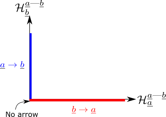
Figure 4: Plot of 2 hospitalities for link ${{\underline{a}}\text{---}{\underline{b}}}$. All allowed values fall in the red or blue regions. If a point falls in the blue region, then the arrow points from ${\underline{a}}$ to ${\underline{b}}$, and if it falls in the red region, then the arrow points from ${\underline{b}}$ to ${\underline{a}}$. If it falls at the origin, then there is no arrow between nodes ${\underline{a}}$ and ${\underline{b}}$.