Convergence of first-order Finite Volume Method based on Exact Riemann Solver for the Complete Compressible Euler Equations
Abstract
Recently developed concept of dissipative measure-valued solution for compressible flows is a suitable tool to describe oscillations and singularities possibly developed in solutions of multidimensional Euler equations. In this paper we study the convergence of the first-order finite volume method based on the exact Riemann solver for the complete compressible Euler equations. Specifically, we derive entropy inequality and prove the consistency of numerical method. Passing to the limit, we show the weak and strong convergence of numerical solutions and identify their limit. The numerical results presented for the spiral, Kelvin-Helmholtz and the Richtmyer-Meshkov problem are consistent with our theoretical analysis.
keywords:
compressible Euler equations, finite volume method, exact Riemann solver, disspipative measure-valued solution, convergence1 Introduction
Hyperbolic conservation laws play an important role in describing many physical and engineering process. An iconic example is the nonlinear system of compressible Euler equations, which governs the dynamics of a compressible material and incorporates mass, momentum and energy conservation.
A characteristic feature of nonlinear conservation laws is that discontinuities (shock waves) may develop after finite time even if the initial condition is smooth. A natural way to overcome this difficulty would be to work with a concept of weak distributional solution. However, it is well-known that such weak solutions fail to be unique. Consequently, the second law of thermodynamics have been proposed as a selection criterion to rule out nonphysical solutions. The entropy production principle have been successfully applied in the scalar multidimensional equations [27] and one-dimensional systems [3, 4]. Unfortunately, it completely fails for multidimensional systems. Recently, De Lellis and Székelyhidi [8] and Chiodaroli et al. [7] showed non-uniqueness of weak entropy solutions for the multidimensional isentropic compressible Euler system, see also [8] for similar non-uniqueness results for the incompressible Euler system. These results have been extended to the complete Euler system in Feireisl et al. [13].
In order to describe oscillations arising in the limits of singular perturbations of hyperbolic conservation laws, a more generalized solution, i.e. measure-valued (MV) solution, was suggested by DiPerna. In 1985 he showed for one-dimensional hyperbolic conservation laws that regularized solutions of associated diffusive and dispersive regularized systems converge to a MV solution, as a regularized parameter vanishes [10]. Recently the concept of MV solution was adapted and applied for multidimensional compressible Euler system [26] and three-dimensional incompressible Euler equations [11], see also [2, 28].
In this paper we work with the concept of dissipative measure-valued (DMV) solution for the complete Euler system, which enjoys the weak-strong uniqueness principle [5]. Analogous concept has been adopted for the insentropic Euler system [23], compressible Navier-Stokes system [12], elastodynamics [9] and other related problems.
In the convergence analysis of numerical schemes for hyperbolic conservation laws the entropy stability plays a crucial role, we refer a reader to a seminal paper of Tadmor [29]. For multidimensional hyperbolic conservation laws the convergence analysis to MV solutions was studied by Fjordholm et al. [22, 21]. For the Lax-Friedrichs and vanishing viscosity finite volume method, Feireisl, Lukáčová and Mizerová generalized the above convergence result for the Euler system and proved the convergence to the DMV solution and the classical solution on its lifespan [15, 14]. For generalization to viscous compressible flows we refer a reader to [17, 18]. In [16, 19] a new tool, -convergence, has been developed to compute strong limits of oscillatory sequences of numerical solutions.
In the present paper we focus on the first-order finite volume method based on the exact Riemann problem solver for the complete compressible Euler system and show its convergence via the concept of DMV solutions. We will only assume that our numerical solutions stay in a physically non-degenerate region, i.e. density is bounded from below and energy is bounded from above. Interestingly, this assumption is equivalent to the strict convexity of the mathematical entropy, see Lemma B.4.
The rest of the paper is organized as follows. In Section 2 we introduce suitable notations and describe the finite volume method with a numerical flux based on the exact solution of the local Riemann problem, cf. Godunov method. In Section 3 we analyze the entropy inequality and give an explicit lower bound of the entropy Hessian matrix, see Appendix B. A crucial step is to show the consistency of our numerical method. Section 4 is devoted to the limiting process. We prove that the numerical solutions will generate a weakly-(*) convergent subsequence and a Young measure, a DMV solution, to the Euler system. Furthermore, employing the theory of -convergence and DMV–strong uniqueness principle, we obtain the strong convergence of the Cesàro averages and strong convergence of numerical solutions to the weak/strong/classical solution. Finally, in Section 5 we present numerical simulations and illustrate the effects of -convergence of numerical solutions. The numerical results clearly demonstrate convergence results being consistent with our analysis. As far as we know this is the first result in literature where the convergence of a well-known Godunov method has been proved rigorously for multidimensional Euler equations.
2 Numerical method
The complete Euler system can be written in the divergence form
| (2.1) |
where denote the conservative vector and flux, defined by
Here denotes density, velocity, momentum, total energy, pressure, internal energy, and the row vector represents the -th row of the unit matrix of size .
Throughout the whole text, we consider the bounded domain together with the space-periodic or no-flux boundary condition. Moreover, the equation of state is restricted to
| (2.2) |
where is the adiabatic constant.
Remark 2.1.
2.1 Spatial discretization and notations
The computational domain consists of rectangular meshes . We denote the set of all mesh cells as , stands for cell face, a unit normal vector to is , the face between two neighboring cells and is denoted by , and the set of all interior faces is given as . Moreover, for we define
| (2.7) |
and introduce the standard average- and jump-operators
| (2.8) |
We use the notation if there exists a generic constant independent on the mesh discretization, such that for .
2.2 Discrete function space and finite volume method
Consider the space of piecewise constant functions
| (2.9) |
We can define the projection
| (2.10) |
where is the Lebesgue measure of .
Let . We consider a semi-discrete finite volume method
| (2.11a) | |||
| (2.11b) | |||
where the numerical flux function is given by means of the exact Riemann solver [30]. Consequently, (2.11a) can be rewritten as
| (2.12) |
where is the solution of a local Riemann problem at face . A piecewise constant solution satisfies an equivalent weak form
| (2.13) |
where .
Remark 2.2.
From here on, we write rather than for , and for . For a two-dimensional uniform mesh a general cell is denoted by with as the center, and . Hence, (2.12) can be rewritten as
where and is the solution at of the following local Riemann problem
and is the solution at of local Riemann problem
3 Consistency
Before proving the consistency of finite volume method (2.13) we formulate a physically reasonable assumption.
Assumption 3.1.
We assume that
| (3.1) |
where are positive constants.
Lemma 3.1.
Under Assumption 3.1 it holds
| (3.2) | |||
| (3.3) |
uniformly for with positive constants , where is the temperature.
Proof.
Here we only give the idea and framework of the proof. More details could be found in [15].
Note that Assumption 3.1 is equivalent to the strict convexity of mathematical entropy function (2.3), see Appendix B.
Lemma 3.2.
Under Assumption 3.1 it holds 111We use the notations and for the -, -norm and the absolute value, respectively.
-
(1)
, , .
-
(2)
with a positive constant .
Here and .
Proof.
Lemma 3.1 implies the boundedness of and .
-
(1)
Since are smooth with respect to and is smooth with respect to , the inequalities in (1) hold.
-
(2)
In [24] Harten proved that is positive definite for all . Assume that in (2) . Then there exists a subsequence satisfying . Since is a bounded set, there exists a subsequence which converges to some . Hence, we get , which is a contradiction.
∎
Remark 3.1.
3.1 Entropy inequality
In [25] Harten proved that the Godunov finite volume method based on the exact solution of the Riemann problem satisfies the entropy inequality (in one-dimensional case)
where is the time-step. Generalizing to multi-dimensions and writing it in the semi-discretization form give
| (3.5) |
Further, we get the equivalent weak form
| (3.6) |
with and .
On the other hand, Chen and Shu in [6] showed that the Godunov finite volume method is entropy stable, i.e.
| (3.7) |
with
Writing explicitly the entropy dissipation we get
| (3.8) |
where
and . Note that matrix is symmetric because is symmetric. Hence, (3.7) implies , i.e., for any . Combining Lemma 3.1 we have uniformly for . Therefore, it holds
which implies the weak BV estimate
| (3.9) |
where is a positive constant depending on . Realizing that represents -seminorm, we have the following interpretation of (3.9). It tells us that
| (3.10) |
3.2 Difference between and
For the sake of convenience, we write in place of . Taking -direction as an example, our strategy is to study the difference between and , where is the solution along the line of the following Riemann problem
| (3.11) |
where are constant. Once is clearly known, then with the definition of , we can directly estimate .
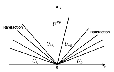
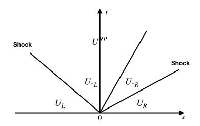
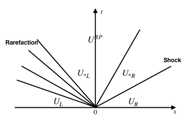
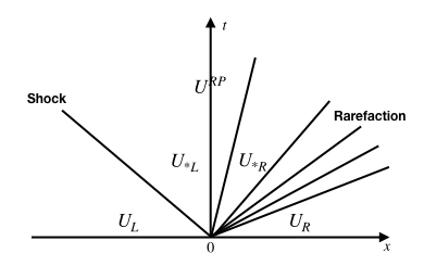
We divide the - domain into four parts separated by the left and right (non-linear) waves and the middle (linear-degenerated) waves. Figure 3.1 shows the possible wave patterns including left rarefaction, right rarefaction; left shock, right shock; left rarefaction, right shock; left shock, right rarefaction. Due to Lemma 3.2, the estimate of reduces to estimating and with and .
Moreover, the Riemann Invariants and Rankine-Hugoniot conditions imply that before the middle wave and after the middle wave. Hence, we only need to study the change of .
3.2.1 Preliminaries
Proposition 3.1.
(solution for and ) The solution for pressure of the Riemann problem (3.11) is given by the root of the algebraic equation
| (3.12) |
where the function is given by
with
| (3.13) | |||
| (3.14) |
The solution for the velocity in the star region is
| (3.15) |
Remark 3.2.
More precisely, satisfy
| (3.16) |
For the right shock the density is found to be
| (3.17) |
and the shock speed is
| (3.18) |
Proposition 3.2.
It holds
| (3.19) |
3.2.2 Estimates
We start by studying the solution inside the rarefaction fan.
Lemma 3.3.
Assume and are connected with the left rarefaction. Denote
as the value inside left rarefaction fan. Then it holds
| (3.20) |
Proof.
Since and are connected with the left rarefaction, then it holds
where is defined in (3.14). From and we have
On the other hand, with the Riemann Invariant we have
which concludes the proof. ∎
Consequently, the value inside left-rarefaction-fan () can be bounded by the left and right side values (). Clearly, it is also true for the right rarefaction wave. Thus, can be controlled by . Hence, we concentrate on and analyze it case by case:
-
(a)
left rarefaction, right rarefaction;
-
(b)
left shock, right shock;
-
(c)
left rarefaction, right shock;
-
(d)
left shock, right rarefaction.
Lemma 3.4 (Left rarefaction, right rarefaction).
Assume the initial data generate left and right rarefaction waves. Then it holds
| (3.21) | |||
| (3.22) | |||
| (3.23) |
where and .
Proof.
Since the initial data generate left and right rarefaction waves, we have
| (3.24) |
and
| (3.25) |
Because of and , it holds
| (3.26) |
which gives
| (3.27) |
Consider the left rarefaction wave. The Riemann Invariant
gives
| (3.28) |
On the other hand, with the help of the Riemann Invariant we have
and
where . Hence, we obtain
Analogously, for the right rarefaction wave we obtain
Consequently,
which concludes the proof. ∎
Lemma 3.5 (Left shock, right shock).
Assume the initial data generate left and right shock waves. Then it holds
| (3.29) | |||
| (3.30) | |||
| (3.31) |
where and .
Proof.
Since the initial data generate left and right shock waves, we have
| (3.32) |
where are the velocities of the left and right shocks respectively. According to
and , we obtain
| (3.33) |
which means
| (3.34) |
Consider the right shock wave. With and
consequently we derive after some algebraic manipulations
Thus,
which gives
Hence, we obtain
On the other hand, using
we obtain
which yields .
Analogously analyzing the left shock wave we obtain
Further, we have
which concludes the proof. ∎
Lemma 3.6 (Left rarefaction, right shock).
Assume the initial data generate left rarefaction waves and right shock waves. Then it holds
| (3.35) | |||
| (3.36) | |||
| (3.37) |
where and .
Proof.
Since the initial data generate left rarefaction waves and right shock waves, we have
| (3.38) |
and
| (3.39) |
This leads to
| (3.40) |
and
| (3.41) |
Consider the right shock wave. Realizing that
we obtain
which also implies . Since satisfies , we have
Consider the left rarefaction wave. Clearly,
On the other hand, with the help of the Riemann Invariant we have
where . Further, we have
which concludes the proof. ∎
Analogously to Lemma 3.6 the following result holds.
Lemma 3.7 (Left shock, right rarefaction).
Assume the initial data generate left shock waves and right rarefaction waves. Then it holds
| (3.42) | |||
| (3.43) | |||
| (3.44) |
where and .
Combining Lemma 3.2 and Lemma 3.4 - 3.7 we finally obtain the following bounds for the Riemann problem solution.
Lemma 3.8.
Remark 3.3.
Lemma 3.8 implies with .
3.3 Consistency
The aim of this section is to prove the consistency of the finite volume method (2.13).
Theorem 3.1.
(Consistency Formulation) Let be the unique solution of the finite volume scheme (2.13) on the time interval with the initial data . Under the Assumption 3.1 we have the following results for all :
-
1.
for all
(3.46) -
2.
for all
(3.47) -
3.
for all
(3.48) -
4.
(3.49)
The errors are bounded by
| (3.50) |
Proof.
Energy conservation for (2.13) follows directly by integrating the discrete energy equation in time and applying the boundary conditions. We proceed by proving (3.46) - (3.48).
Realizing that
| (3.53) |
we obtain after some manipulations
For the last equality, we have used the Gauss theorem and the no-flux or periodic boundary condition
| (3.54) |
Let us now consider the error terms
Applying Lemma 3.2, i.e. and the fact
we have the following estimate
Realizing that
we derive
4 Convergence
In order to keep the paper self-contained we present the definition of a dissipative measure-valued solution for the Euler system (2.1), (2.6), cf. [18].
Definition 4.1.
Let be a bounded domain. A parametrized probability measure ,
is called a dissipative measure-valued (DMV) solution of the Euler system (2.1), (2.6) with the space-periodic or no-flux boundary condition and initial condition if the following holds:
-
1.
(lower bound on density and entropy)
(4.1) -
2.
(energy inequlity) the integral inequality
(4.2) holds for a.a. with the energy concentration defect
-
3.
(equation of continuity)
and the integral equality
(4.3) for any and any ;
-
4.
(momentum equation)
and the integral equality
(4.4) for any and any , ( also satisfies when no-flux boundary condition is used), where the Reynolds concentration defect
satisfies
(4.5) -
5.
(entropy balance)
and the integral inequality
(4.6) for any and any .
Remark 4.1.
Consider a family of numerical solutions generated by our finite volume method (2.13). We note that a sequence can be mapped uniquely to a sequence . Due to Theorem 3.1 is a consistent approximation of complete Euler system. Consequently, up to a subsequence generates the Young measure , which is a disspative measure-valued solution of the Euler system in the sense of Definition 4.1. Following [18] the concentration defects are
with
Theorem 4.1.
(Weak convergence)
Proof.
Under Assumption 3.1 Lemma 3.1 gives
Applying the Fundamental Theorem on Young Measure [1] implies the existence of a convergent subsequence and a parameterized probability measure satisfying that weakly-(*) converges to in . Moreover,
weakly-(*) converge to
in , respectively. Consequently, the concentration defects vanish, i.e. .
Hence, passing to the limit , (3.46) in Theorem 3.1 gives
| (4.8) |
for . Analogously, (2) and (3.48) in Theorem 3.1 yield
for and for no-flux boundary condition, and
| (4.9) |
for , respectively. Finally, (3.49) in Theorem 3.1 implies
| (4.10) |
and concludes that is a DMV solution of the complete Euler system. ∎
Having shown weak convergence to a DMV solution allows us to look for strong convergence to the observable quantities, such as the expected value and first variance. To this end we apply a novel technique of -convergence as introduced in [16, 18].
Theorem 4.2.
(-convergence)
Applying techniques developed in [18] we directly obtain the following strong convergence results.
Theorem 4.3.
(Strong convergence)
Let be the family of numerical solutions obtained by the finite volume method (2.13) and with initial data . Let Assumption 3.1 hold. Let the subsequence
in the sense specified in Theorem 4.1, where the barycenters , and . Then the following holds:
-
1.
weak solution
If is a weak entropy solution of the Euler system with initial data , then
and the strong convergence holds, i.e.
for any .
-
2.
classical solution
Let be a bounded Lipschitz domain and such that
Then is a classical solution to the Euler system and
for any .
-
3.
strong solution
Let periodic boundary conditions are applied. Suppose that the Euler system admits a strong solution in the class
emanating from initial data . Then it holds
for any .
5 Numerical results
In this section we simulate a spiral problem, i.e. two-dimensional Riemann problem, Kelvin-Helmholtz problem and Richtmyer-Meshkov problem [22, 21] to illustrate the weak, strong and -convergence of the finite volume method (2.13).
In our computations the computational domain is and divided into uniform cells. Denote the Cesàro average of the numerical solutions and their first variance
respectively. Let be the reference solution computed on the finest mesh with cells. Analogously to [19] we compute four errors
| (5.1) |
where is the Cesàro average of the Dirac measures concentrated on numerical solution . In addition, we apply the outflow boundary condition to the spiral problem and periodic boundary condition to the other two problems. Moreover, the CFL number is set to and the adiabatic index is taken as .
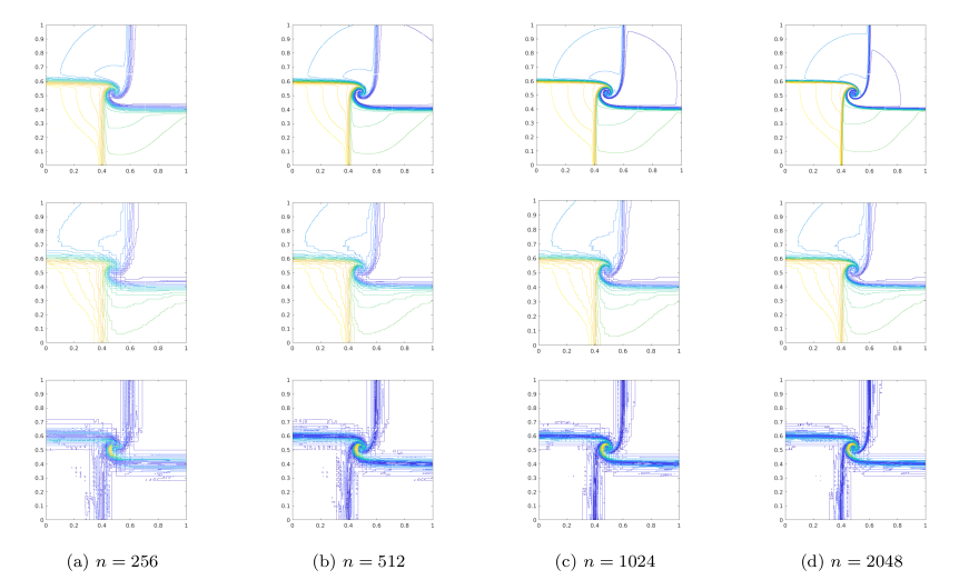
Example 5.1 (Spiral problem).
We consider one of the classical 2D Riemann problem with the initial data
This problem describes the interaction of four contact discontinuities (vortex sheets) with the negative sign. As time increases the four initial vortex sheets interact each other to form a spiral with the low density around the center of the domain. This is a typical cavitation phenomenon well-known in gas dynamics. We compute the solution up to the finite time .
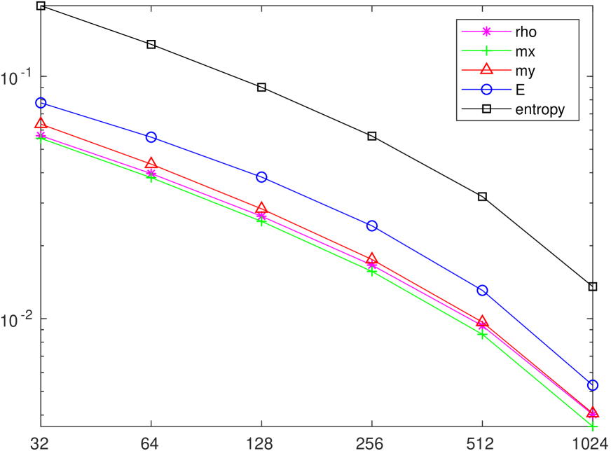
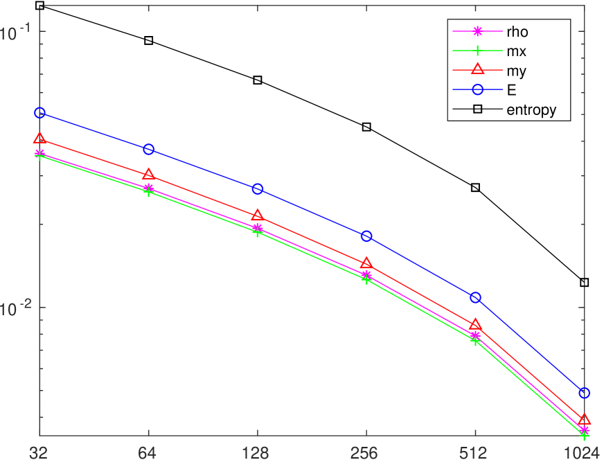
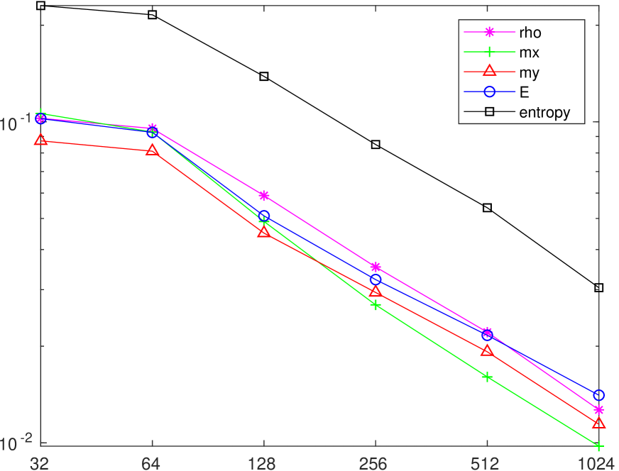
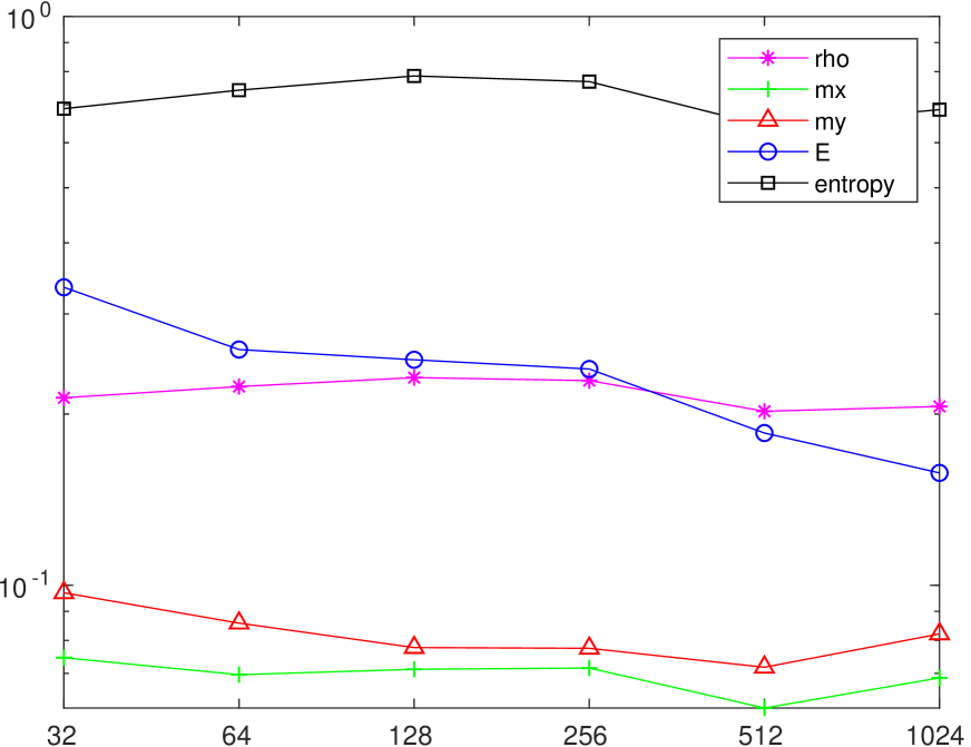
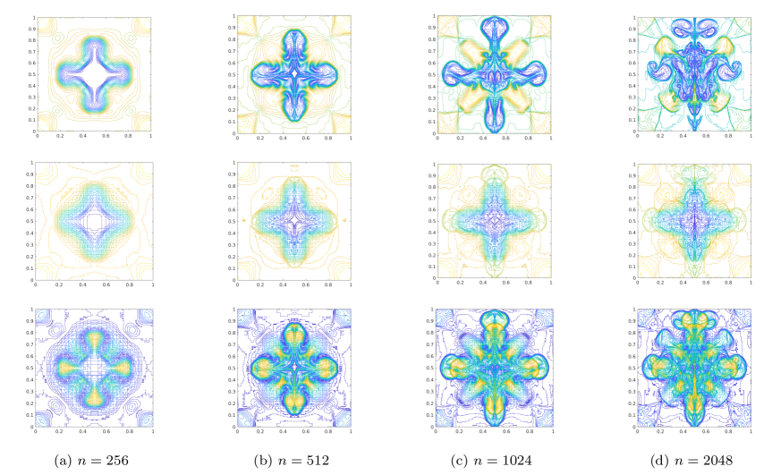
Figure 5.1 shows the errors of obtained on different meshes and the reference solution on a mesh with cells. The errors of are specifically listed in Tables 5.1, 5.2, respectively. Moreover, Figures 5.2, 5.3 show the contour of and obtained on different meshes, respectively.
The numerical results show that four errors are all decreasing with the refinement of mesh. This together with the pictures of the first variance indicate that and the numerical solutions converge to the weak solution. This is in accordance with our theoretical results. We point out that the convergence rate is 1.
| error | order | error | order | error | order | error | order | |
|---|---|---|---|---|---|---|---|---|
| 32 | 0.0569 | - | 0.0361 | - | 0.0179 | - | 0.0367 | - |
| 64 | 0.0397 | 0.5189 | 0.0270 | 0.4206 | 0.0102 | 0.8165 | 0.0272 | 0.4354 |
| 128 | 0.0265 | 0.5854 | 0.0193 | 0.4795 | 0.0078 | 0.3810 | 0.0195 | 0.4790 |
| 256 | 0.0166 | 0.6698 | 0.0131 | 0.5655 | 0.0055 | 0.5199 | 0.0132 | 0.5626 |
| 512 | 0.0093 | 0.8316 | 0.0079 | 0.7299 | 0.0036 | 0.6089 | 0.0080 | 0.7258 |
| 1024 | 0.0040 | 1.2172 | 0.0036 | 1.1388 | 0.0016 | 1.1319 | 0.0036 | 1.1311 |
| error | order | error | order | error | order | error | order | |
|---|---|---|---|---|---|---|---|---|
| 32 | 0.1956 | - | 0.1242 | - | 0.0619 | - | 0.1263 | - |
| 64 | 0.1355 | 0.5297 | 0.0927 | 0.4216 | 0.0360 | 0.7841 | 0.0933 | 0.4372 |
| 128 | 0.0901 | 0.5882 | 0.0666 | 0.4771 | 0.0278 | 0.3734 | 0.0669 | 0.4800 |
| 256 | 0.0567 | 0.6692 | 0.0451 | 0.5634 | 0.0194 | 0.5150 | 0.0453 | 0.5632 |
| 512 | 0.0319 | 0.8297 | 0.0272 | 0.7294 | 0.0125 | 0.6370 | 0.0274 | 0.7267 |
| 1024 | 0.0136 | 1.2341 | 0.0123 | 1.1417 | 0.0057 | 1.1396 | 0.0125 | 1.1346 |
Example 5.2 (Kelvin-Helmholtz problem).
We consider a shear flow of three fluid layers with different densities. The initial data are given by
where the interface profiles
are chosen to be small perturbations around the lower and the upper interfaces, respectively. Moreover,
where and are arbitrary, but fixed numbers. The coefficients have been normalized such that to guarantee that for . In the simulation we have , and .
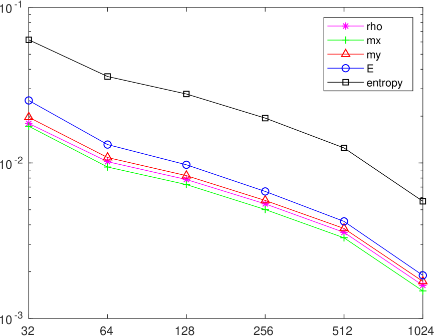
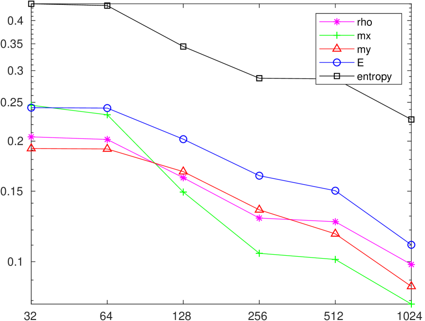
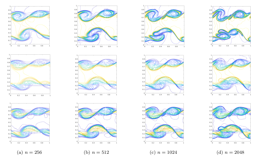
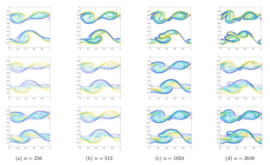
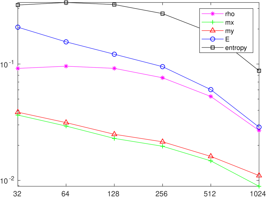
Figure 5.4 shows the errors of obtained on different meshes. Tables 5.3, 5.4 present the errors of , respectively. Moreover, Figures 5.5, 5.6 show the contours of and obtained on different meshes, respectively.
The numerical results show that the numerical solutions obtained by the finite volume method (2.13) seem to converge in the sense of . Though, the concergence rates of are much higher than that of .
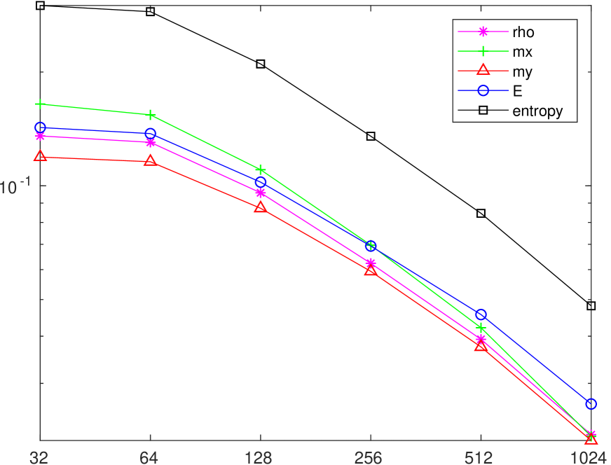
| error | order | error | order | error | order | error | order | |
|---|---|---|---|---|---|---|---|---|
| 32 | 0.2050 | - | 0.1307 | - | 0.1026 | - | 0.1355 | - |
| 64 | 0.2020 | 0.0215 | 0.1265 | 0.0468 | 0.0953 | 0.1052 | 0.1303 | 0.0561 |
| 128 | 0.1621 | 0.3175 | 0.0918 | 0.4620 | 0.0589 | 0.6939 | 0.0958 | 0.4437 |
| 256 | 0.1285 | 0.3345 | 0.0584 | 0.6542 | 0.0353 | 0.7393 | 0.0623 | 0.6202 |
| 512 | 0.1259 | 0.0303 | 0.0357 | 0.7072 | 0.0221 | 0.6750 | 0.0392 | 0.6682 |
| 1024 | 0.0984 | 0.3549 | 0.0185 | 0.9533 | 0.0127 | 0.8033 | 0.0219 | 0.8381 |
| error | order | error | order | error | order | error | order | |
|---|---|---|---|---|---|---|---|---|
| 32 | 0.4405 | - | 0.2950 | - | 0.2302 | - | 0.3000 | - |
| 64 | 0.4359 | 0.0152 | 0.2854 | 0.0479 | 0.2155 | 0.0952 | 0.2889 | 0.0543 |
| 128 | 0.3446 | 0.3392 | 0.2021 | 0.4980 | 0.1385 | 0.6375 | 0.2102 | 0.4593 |
| 256 | 0.2871 | 0.2631 | 0.1244 | 0.6998 | 0.0850 | 0.7052 | 0.1353 | 0.6355 |
| 512 | 0.2860 | 0.0055 | 0.0747 | 0.7356 | 0.0540 | 0.6544 | 0.0846 | 0.6779 |
| 1024 | 0.2265 | 0.3366 | 0.0389 | 0.9423 | 0.0304 | 0.8274 | 0.0481 | 0.8135 |
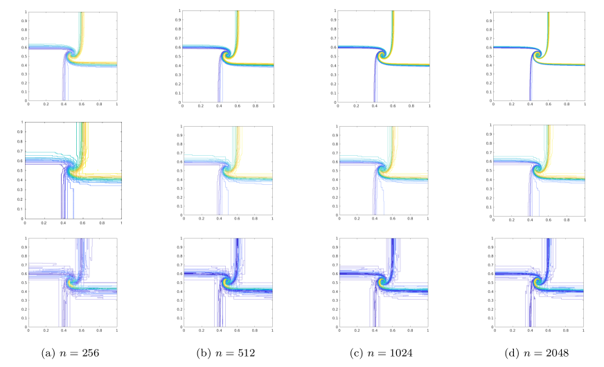
Example 5.3 (Richtmyer-Meshkov problem).
This example describes complex interactions of strong shocks with unstable interfaces. The initial data are given by
where and the radial interface is perturbed by
with . The parameters are arbitrary, but fixed numbers chosen such that and . In the simulation we set and .
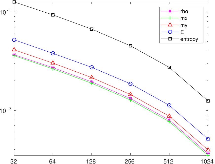
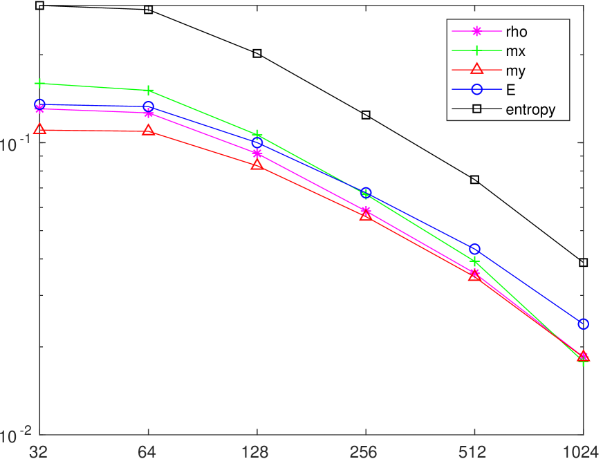
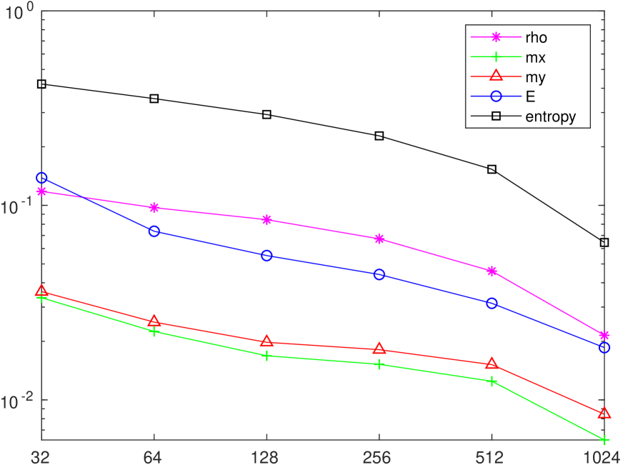
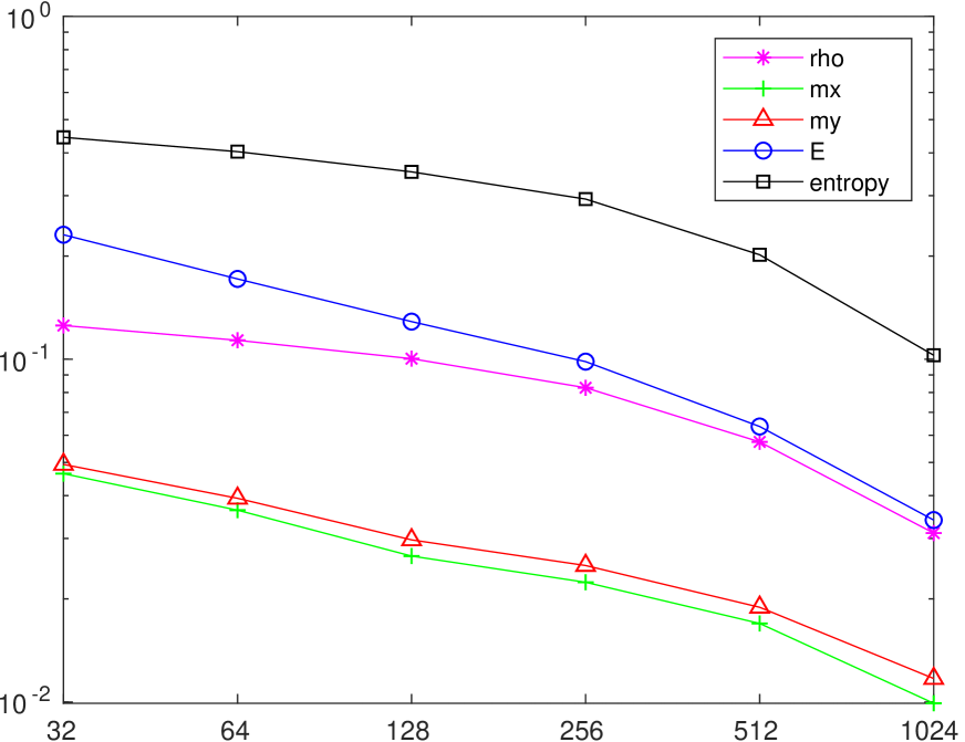
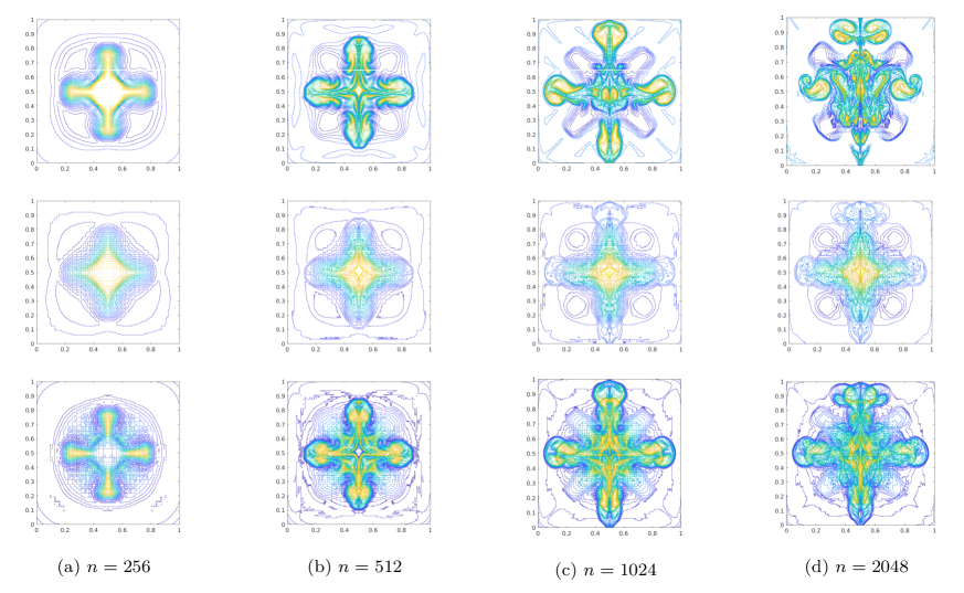
Figure 5.7 shows the errors of obtained using different meshes , see also Tables 5.5, 5.6. Moreover, the contours of and are shown in Figures 5.8, 5.9, respectively.
The figures and tables clearly indicate only a weak converge of single simulations obtained by the finite volume method (2.13). Indeed, the numerical solutions do not converge strongly in -norm. On the other hand, the Cesàro average and the first variance of the numerical solutions, as well as the Wasserstein distance of the corresponding Dirac distributions converge strongly in -norm. These results again confirm our theoretical analysis on the convergence of the finite volume method (2.13). In the Richtmyer-Meshkov case the limiting solution is not a weak solution but a dissipative measure-valued solution.
| error | order | error | order | error | order | error | order | |
|---|---|---|---|---|---|---|---|---|
| 32 | 0.2136 | - | 0.0917 | - | 0.1180 | - | 0.1254 | - |
| 64 | 0.2236 | -0.0656 | 0.0958 | -0.0626 | 0.0973 | 0.2774 | 0.1136 | 0.1433 |
| 128 | 0.2318 | -0.0523 | 0.0918 | 0.0613 | 0.0844 | 0.2051 | 0.1004 | 0.1782 |
| 256 | 0.2290 | 0.0175 | 0.0762 | 0.2692 | 0.0673 | 0.3274 | 0.0826 | 0.2816 |
| 512 | 0.2023 | 0.1790 | 0.0526 | 0.5337 | 0.0459 | 0.5512 | 0.0574 | 0.5249 |
| 1024 | 0.2063 | -0.0280 | 0.0269 | 0.9694 | 0.0215 | 1.0959 | 0.0311 | 0.8835 |
| error | order | error | order | error | order | error | order | |
|---|---|---|---|---|---|---|---|---|
| 32 | 0.6887 | - | 0.3215 | - | 0.4205 | - | 0.4440 | - |
| 64 | 0.7423 | -0.1082 | 0.3378 | -0.0716 | 0.3539 | 0.2487 | 0.4032 | 0.1391 |
| 128 | 0.7862 | -0.0830 | 0.3246 | 0.0578 | 0.2931 | 0.2718 | 0.3521 | 0.1957 |
| 256 | 0.7684 | 0.0330 | 0.2713 | 0.2588 | 0.2277 | 0.3646 | 0.2932 | 0.2639 |
| 512 | 0.6425 | 0.2582 | 0.1869 | 0.5373 | 0.1533 | 0.5704 | 0.2017 | 0.5396 |
| 1024 | 0.6860 | -0.0945 | 0.0876 | 1.0943 | 0.0645 | 1.2502 | 0.1027 | 0.9737 |
6 Conclusions
We have shown the convergence of the Godunov finite volume method (2.13), which is based on the exact solution of a local Riemann problem for the complete compressible Euler system. Hereby we have only assumed that our numerical solutions belong to a physically non-degenerate region, i.e. we have a uniform lower bound on density and an upper bound on energy. The latter is equivalent to the existence of a uniform lower bound on entropy Hessian matrix, see Lemma B.4. Using the fact that the finite volume method (2.13) is entropy stable, the entropy inequality together with the explicit lower bound of the entropy Hessian matrix yield the weak BV estimate (3.9). Further, we have shown that the difference between the exact solution of the local Riemann problem and its initial data, i.e. numerical solution at time , can be controlled by the jump of numerical solution itself. Consistency of the method is proved in Theorem 3.1. Weak convergence to a generalized solution, the dissipative measure-valued (DMV) solution, is showed in Theorem 4.1. Applying the novel tool of -convergence we obtained strong convergence to the expected value and first variance of a dissipative measure-valued solution, see Theorem 4.2. Theorem 4.3 summarizes the cases of strong convergence of numerical solutions of (2.13). The latter happens if the limit is a weak or solution to the Euler system (2.1). In addition, applying the DMV-strong uniqueness principle [5] we also have strong convergence of our numerical solutions on the lifespan of the strong solution.
Numerical results for the spiral problem, the Kelvin-Helmholtz problem and the Richtmyer-Meshkov problem confirm results of theoretical analysis. In particular, we observe that for highly oscillatory limit, as is the case of the Richtmyer-Meshkov test, single numerical solutions do not converge strongly. On the other hand, we obtain the strong convergence of observable quantities, i.e. the expected values and first variances.
Although the Godunov finite volume method is one of the most classical schemes for hyperbolic conservation laws, its numerical analysis for multidimensional systems still remains open in general. The main goal of this paper was to fill this gap and illustrate the application of the recently developed concepts of generalized DMV solution and -convergence on an iconic example, the multidimensional Euler system. In future it will be interesting to extend the obtained results to general multidimensional hyperbolic conservation laws.
Acknowledgments
M.L. has been funded by the German Science Foundation (DFG) under the collaborative research projects TRR SFB 165 (Project A2) and TRR SFB 146 (Project C5). Y.Y. has been funded by Sino-German (CSC-DAAD) Postdoc Scholarship Program in 2020 - Project number 57531629.
References
- [1] J. M. Ball. A version of the fundamental theorem for young measures. In PDEs and Continuum Models of Phase Transitions, pages 207–215. Springer, 1989.
- [2] Y. Brenier, C. De Lellis, and L. Székelyhidi. Weak-strong uniqueness for measure-valued solutions. Commun. Math. Phys., 305(2):351–361, 2011.
- [3] A. Bressan, G. Crasta, and B. Piccoli. Well-Posedness of the Cauchy Problem for Systems of Conservation Laws. Memoirs of the American Mathematical Society, 2000.
- [4] A. Bressan and M. Lewicka. A uniqueness condition for hyperbolic systems of conservation laws. Discrete Contin. Dyn. Syst., 6(3):673–682, 2000.
- [5] J. Březina and E. Feireisl. Measure-valued solutions to the complete Euler system. J. Math. Soc. Japan, 70(4):1227 – 1245, 2018.
- [6] T.H. Chen and C.W. Shu. Entropy stable high order discontinuous Galerkin methods with suitable quadrature rules for hyperbolic conservation laws. J. Comput. Phys., 345(15):427–461, 2017.
- [7] E. Chiodaroli, C. De Lellis, and O. Kreml. Global ill-posedness of the isentropic system of gas dynamics. Commun. Pure Appl. Math., 68(7):1157–1190, 2015.
- [8] C. De Lellis and L. Székelyhidi Jr. On admissibility criteria for weak solutions of the Euler equations. Arch. Ration. Mech. Anal., 195(1):225–260, 2010.
- [9] S. Demoulini, D. M. A. Stuart, and A. E. Tzavaras. Weak–strong uniqueness of dissipative measure-valued solutions for polyconvex elastodynamics. Arch. Ration. Mech. Anal., 205(3):927–961, 2012.
- [10] R.J. DiPerna. Measure-valued solutions to conservation laws. Arch. Ration. Mech. Anal., 88(3):223–270, 1985.
- [11] R.J. DiPerna and A.J. Majda. Oscillations and concentrations in weak solutions of the incompressible fluid equations. Commun. Math. Phys., 108(4):667–689, 1987.
- [12] E. Feireisl, P. Gwiazda, A. Świerczewska Gwiazda, and E. Wiedemann. Dissipative measure-valued solutions to the compressible Navier–Stokes system. Calc. Var. Part. Diff. Eq., 55(6):141, 2016.
- [13] E. Feireisl, C. Klingenberg, O. Kreml, and S. Markfelder. On oscillatory solutions to the complete Euler system. J. Differ. Equ., 269(2):1521–1543, 2020.
- [14] E. Feireisl, M. Lukáčová-Medvid’ová, and H. Mizerová. A finite volume scheme for the Euler system inspired by the two velocities approach. Numer. Math., 144(1):89–132, 2020.
- [15] E. Feireisl, M. Lukáčová-Medvid’ová, and H. Mizerová. Convergence of finite volume schemes for the Euler Equations via dissipative measure-valued solutions. Found. Comput. Math., 20(4):923–966, 2020.
- [16] E. Feireisl, M. Lukáčová-Medvid’ová, and H. Mizerová. -convergence as a new tool in numerical analysis. IMA J. Numer. Anal., 40(4):2227–2255, 2020.
- [17] E. Feireisl, M. Lukáčová-Medvid’ová, H. Mizerová, and B. She. Convergence of a finite volume scheme for the compressible Navier-Stokes system. ESAIM Math. Model. Numer. Anal., 53(6):1957–1979, 2019.
- [18] E. Feireisl, M. Lukáčová-Medvid’ová, H. Mizerová, and B. She. Numerical Analysis of Compressible Flows. Springer, in print, 2021.
- [19] E. Feireisl, M. Lukáčová-Medvid’ová, B. She, and Y. Wang. Computing oscillatory solutions of the Euler system via -convergence. Math. Models Methods Appl. Sci., 2021.
- [20] M. Feistauer, J. Felcman, and I. Straškraba. Mathematical and computational methods for compressible flow. Numerical Mathematics and Scientific Computation. The Clarendon Press, Oxford University Press, Oxford, 2003.
- [21] U.S. Fjordholm, R. Käppeli, S. Mishra, and E. Tadmor. Construction of approximate entropy measure-valued solutions for hyperbolic systems of conservation laws. Found. Comput. Math., 17(3):763–827, 2017.
- [22] U.S. Fjordholm, S. Mishra, and E. Tadmor. On the computation of measure-valued solutions. Acta Numer., 25:567–679, 2016.
- [23] P. Gwiazda, A. Świerczewska-Gwiazda, and E Wiedemann. Weak-strong uniqueness for measure-valued solutions of some compressible fluid models. Nonlinearity, 28(11):3873–3890, 2015.
- [24] A. Harten. On the symmetric form of systems of conservation laws with entropy. J. Comput. Phys., 49(1):151–164, 1983.
- [25] A. Harten, P.D. Lax, and B. Van Leer. On upstream differencing and Godunov-type schemes for hyperbolic conservation laws. SIAM Rev., 25(1):35–61, 1983.
- [26] D. Kröner and W. Zajaczkowski. Measure-valued solutions of the Euler equations for ideal compressible polytropic fluids. Math. Methods Appl. Sci., 19(3):235–252, 1996.
- [27] S. Kružkov. First order quasilinear equations in several independent variables. USSR Math. Sbornik, 10(2):217–243, 1970.
- [28] J. Málek, J. Nečas, M. Rokyta, and M. Růžička. Weak and Measure-valued Solutions to Evolutionary PDEs. Chapman annd Hall/CRC, 2019.
- [29] E. Tadmor. The numerical viscosity of entropy stable schemes for systems of conservation laws. I. Math. Comp., 49(179):91–103, 1987.
- [30] E.F. Toro. Riemann Solver and Numerical Methods for Fluid Dynamics, Third edition. Springer-Verlag Berlin Heidelberg, 2009.
A Lipschitz continuity of
The aim of this section is to give the estimates of , also denoted by .
Lemma A.1.
It holds
| (A.1) | |||
| (A.2) |
Proof.
If then . After some calculations we obtain
Moreover, we obtain
which concludes the proof. ∎
Lemma A.2.
It holds
| (A.3) | |||
| (A.4) |
Proof.
Some manipulations give
which implies
On the other hand, we have
which gives
Consequently, we obtain
which concludes the proof. ∎
Lemma A.3.
It holds
B Lower bound of the entropy Hessian matrix
In this section we give the lower bound of entropy Hessian matrix for . Harten [24] has already given the explicit expression of in two-dimensional case. Analogously, we can obtain its three-dimensional explicit expression with
where
Moreover, the symmetric matrix is positive definite if and only if .
Consider the special case , i.e., and . After some calculations we obtain the characteristic function of the matrix
where
Taking derivation of gives
Denote the roots of by with , the roots of by and with
| (B.1) |
As known, is positive definite [24], which implies
| (B.2) |
Lemma B.1.
It holds
| (B.3) |
Proof.
Denote by , i.e., . Then implies
| (B.4) |
It is easy to show that
Since
we have .
On the other hand, we have
Hence,
which concludes the proof. ∎
Lemma B.2.
It holds
| (B.5) |
Proof.
Let . From Lemma B.1 we know that the lower boundary of can only be found within . With the definition of the following decomposition gives
where the first inequality holds since , and the second inequality due to . Hence, if satisfies
then . This concludes the proof since . ∎
Summarizing, we have the estimate for the smallest eigenvalue of the entropy Hessian matrix .
Lemma B.3.
It holds
| (B.6) |
where represents the eigenvalue of matrix and .
Specially, stand here for the infimum and supremum, respectively. For example,
| (B.7) |
where represents the eigenvalue of matrix .
Lemma B.4.
The following is equivalent:
-
(i)
for a.e. ;
-
(ii)
for a.e. .
Proof.
Step 1: Suppose that (i) holds. Combining Lemma 3.1 and Lemma B.3 we have
where and are defined in the proof of Lemma 3.1.
Step 2: Let (ii) hold. From (B.6) we obtain
| (B.8) |
In the following, with the relationship
| (B.9) |
we show (i) by contradiction.
-
1.
.
Let fixed. It is the fact that only depends on , which implies fixed. Hence, we can derive from (B.9).
-
2.
.
Let fixed. With we obtain . Letting gives the behavior of
Combining implies or , which is a contradiction with .
-
3.
.
Let fixed. With we obtain . Call back that
We let , which implies that satisfies and . Passing to the limit , i.e. , we obtain , which is a contradiction.
Consequently, it holds , which concludes the proof. ∎