UVIP: Model-Free Approach to Evaluate Reinforcement Learning Algorithms

Abstract

Policy evaluation is an important instrument for the comparison of different algorithms in Reinforcement Learning (RL). Yet even a precise knowledge of the value function $V^{\pi}$ corresponding to a policy $\pi$ does not provide reliable information on how far is the policy $\pi$ from the optimal one. We present a novel model-free upper value iteration procedure (UVIP) that allows us to estimate the suboptimality gap $V^{\star}(x)-V^{\pi}(x)$ from above and to construct confidence intervals for $V^{\star}$. Our approach relies on upper bounds to the solution of the Bellman optimality equation via martingale approach. We provide theoretical guarantees for UVIP under general assumptions and illustrate its performance on a number of benchmark RL problems.

1 Introduction

The key objective of Reinforcement Learning (RL) is to learn an optimal agent’s behaviour in an unknown environment. A natural performance metric is given by the value function $V^{\pi}$ which is expected total reward of the agent following $\pi$. There are efficient algorithms to evaluate this quantity, e.g. temporal difference methods Sutton (1988), Tsitsiklis and Van Roy (1997). Unfortunately, even a precise knowledge of $V^{\pi}$ does not provide reliable information on how far is the policy $\pi$ from the optimal one. To address this issue a popular quality measure is the regret of the algorithm that is the difference between the total sum of rewards accumulated when following the optimal policy and the sum of rewards obtained when following the current policy $\pi$ (see e.g. Jaksch et al. (2010)). In the setting of finite state- and action space Markov Decision Processes (MDP) there is a variety of regret bounds for popular RL algorithms like Q-learning Jin et al. (2018), optimistic value iteration Azar et al. (2017), and many others.

Unfortunately, regret bounds beyond the discrete setup are much less common in the literature. Even more crucial drawback of the regret-based comparison is that regret bounds are typically pessimistic and rely on the unknown quantities of the underlying MDP’s. A simpler, but related, quantity is the suboptimality gap (policy error) $\Delta_{\pi}(x)\doteq V^{\star}(x)-V^{\pi}(x)$. Since we do not know $V^{\star}$, the suboptimality gap can not be calculated directly. There is a vast amount of literature devoted to theoretical guarantees for $\Delta_{\pi}(x)$, see e.g. Antos et al. (2007), Szepesvári (2010), Pires and Szepesvári (2016) and references therein. However, these bounds share the same drawbacks as the regret bounds. Moreover, known bounds does not apply to the general policy $\pi$ and depends heavily on the particular algorithm which produced it. For instance, in Approximate Policy Iteration (API, Bertsekas and Tsitsiklis (1996)) all existing bounds for $\Delta_{\pi}(x)$ depend on the one-step error induced by the approximation of the action-value function. This one-step error is difficult to quantify since it depends on the unknown smoothness properties of the action-value function. Similarly, in policy gradient methods (see e.g. Sutton and Barto (2018)), there is always an approximation error due to the choice of family of policies that can be hardly quantified. The approach based on the policy optimism principle (see Efroni et al. (2019)) suggests to initialise the value iteration algorithm using an upper bound (optimistic value) for $V^{\star}$, yielding a sequence of upper bounds converging to $V^{\star}$. However this approach is tailored to finite state- and action space MDPs and is not applicable to evaluate the quality of the general policy $\pi$. To summarise, such bounds can not be used to construct tight model-free confidence bounds for $V^{\star}.$

In this paper we are interested in deriving agnostic (model independent) bounds for the policy error using the concept of upper solutions to the Bellman optimality equation. Our approach is substantially different from the ones known in literature as it can be used to evaluate performance bounds for arbitrary given policy $\pi$. The concept of upper solutions is closely related to martingale duality in optimal control and information relaxation approach, see Belomestny and Schoenmakers (2018), Rogers (2007) and references therein. This idea has been successfully used in the recent paper Shar and Jiang (2020). This work proposes to use the duality approach to improve the performance of Q-learning algorithm in finite horizon MDP through the use of “lookahead” upper and lower bounds. Compared to Shar and Jiang (2020), our approach is not restricted to the Q-learning. The concept of upper solutions has also a connection to distributional RL, as it can be formulated pathwise or using distributional Bellman operator, see e.g. Lyle et al. (2019). A further study of this connection is a promising future research area.

Contributions and Organization

The contributions of this paper are three-fold:

• We propose a novel approach to construct model free confidence bounds for the optimal value function $V^{\star}$ based on a notion of upper solutions.

• Given a policy $\pi,$ we propose an upper value iterative procedure (UVIP) for constructing an (almost sure) upper bound for $V^{\pi}$ such that it coincides with $V^{\star}$ if $\pi=\pi^{\star}.$

• We study convergence properties of the approximate UVIP in the case of general state and action spaces. In particular, we show that the variance of the resulting upper bound is small if $\pi$ is close to $\pi^{*}$ leading to the tight confidence bounds for $V^{\star}$.

The paper is organized as follows. First, in section 2, we briefly recall main concepts related with the MDPs, and introduce some notations. Then in sections 3 and 4 we introduce the framework of UVIP and discuss its basic properties. In section 5 we perform theoretical study of the approximate UVIP. Numerical results are collected in section 6. Section 7 concludes the paper. Section 8 in appendix is devoted to the proof of main theoretical results.

Notations and definitions

For $N\in\mathbb{N}$ we define $[N]\doteq\{1,\ldots,N\}$. Let us denote the space of bounded measurable functions with domain $\mathsf{X}$ by $\mathcal{B}(\mathsf{X})$ equipped with the norm $\|f\|_{\mathsf{X}}=\sup_{x\in\mathsf{X}}|f(x)|$ for any $f\in\mathcal{B}(\mathsf{X}).$ In what follows, whenever a norm is uniquely identifiable from its argument, we will drop the index of the norm denoting the underlying space. We denote by ${\rm P}^{a}$ an $\mathcal{B}(\mathsf{X})\to\mathcal{B}(\mathsf{X})$ operator defined by $({\rm P}^{a}V)(x)=\int V(x^{\prime}){\rm P}^{a}(dx^{\prime}|x)$. For an arbitrary metric space $(\mathcal{X},\rho_{\mathcal{X}})$ and function $f:\mathcal{X}\to\mathbb{R}$ we define by $\mathrm{Lip}_{\rho_{\mathcal{X}}}(f)\doteq\sup_{x\neq y}|f(x)-f(y)|/\rho_{\mathcal{X}}(x,y)$.

2 Preliminary

A Markov Decision Process (MDP) is a tuple $(\mathsf{X},\mathsf{A},\mathcal{P},r)$, where $\mathsf{X}$ is the state space, $\mathsf{A}$ is the action space, $\mathcal{P}=({\rm P}^{a})_{a\in\mathsf{A}}$ is the transition probability kernel and $r=(r^{a})_{a\in\mathsf{A}}$ is the reward function. For each state $x\in\mathsf{X}$ and action $a\in\mathsf{A}$, ${\rm P}^{a}(\cdot|x)$ stands for a distribution over the states in $\mathsf{X}$, that is, the distribution over the next states given that action $a$ is taken in the state $x$. For each action $a\in\mathsf{A}$ and state $x\in\mathsf{X}$, $r^{a}(x)$ gives a reward received when action $a$ is taken in state $x$. An MDP describes the interaction of an agent and its environment. When an action $A_{t}\in\mathsf{A}$ at time $t$ is chosen by the agent, the state $X_{t}$ transitioned to $X_{t+1}\sim{\rm P}^{A_{t}}(\cdot|X_{t})$. The agent’s goal is to maximize the expected total discounted reward, $\mathsf{E}[\sum_{t=0}^{\infty}\gamma^{t}r^{A_{t}}(X_{t})]$, where $0<\gamma<1$ is the discount factor. A rule describing the way an agent acts given its past actions and observations is called a policy. The value function of a policy $\pi$ in a state $x\in\mathsf{X}$, denoted by $V^{\pi}(x)$, is $V^{\pi}(x)=\mathsf{E}[\sum_{t=0}^{\infty}\gamma^{t}r^{A_{t}}(X_{t})|X_{0}=x]$, that is, the expected total discounted reward when the initial state ($X_{0}=x$) assuming the agent follows the policy $\pi$. Similarly, we define the action-value function $Q^{\pi}(x,a)=\mathsf{E}[\sum_{t=0}^{\infty}\gamma^{t}r^{A_{t}}(X_{t})|X_{0}=x,A_{0}=a]$. An optimal policy is one that achieves the maximum possible value amongst all policies in each state $x\in\mathsf{X}$. The optimal value for state $x$ is denoted by $V^{\star}(x)$. A deterministic Markov policy can be identified with a map $\pi:\mathsf{X}\to\mathsf{A}$, and the space of measurable deterministic Markov policies will be denoted by $\Pi$. When, in addition, the reward function is bounded, which we assume from now on, all the value functions are bounded and one can always find a deterministic Markov policy that is optimal Puterman (2014). We also define a greedy policy w.r.t. action-value function $Q(x,a)$, which is a deterministic policy $\pi(x)\in\operatorname*{argmax}_{a\in\mathsf{A}}Q(x,a)$. The Bellman return operator w.r.t. ${\rm P}$, $\mathsf{T}_{{\rm P}}:\mathcal{B}(\mathsf{X})\to\mathcal{B}(\mathsf{X}\times\mathsf{A})$, is defined by $(\mathsf{T}_{{\rm P}}V)(x,a)=r^{a}(x)+\gamma{\rm P}^{a}V(x)$ and the maximum selection operator $\mathsf{M}:\mathcal{B}(\mathsf{X}\times\mathsf{A})\rightarrow\mathcal{B}(\mathsf{X})$ is defined by $(\mathsf{M}V^{\cdot})(x)=\max_{a}V^{a}(x)$. Then $\mathsf{M}\mathsf{T}_{{\rm P}}$ corresponds to the Bellman optimality operator, see Puterman (2014). The optimal value function $V^{\star}$ satisfies a non-linear fixed-point equation

$$\textstyle{V^{\star}(x)=\mathsf{M}\mathsf{T}_{{\rm P}}V^{\star}(x).}$$ (1)

which is known as the Bellman optimality equation. We write $Y^{x,a},x\in\mathsf{X},a\in\mathsf{A}$ for a random variable generated according to ${\rm P}^{a}(\cdot|x)$, and define a random Bellman operator $(\widetilde{\mathsf{T}}_{{\rm P}}V)(x)\mapsto r^{a}(x)+\gamma V(Y^{x,a})$. We say that a (deterministic) policy $\pi$ is greedy w.r.t. a function $V\in\mathcal{B}(\mathsf{X})$ if, for all $x\in\mathsf{X}$

$$\textstyle{\pi(x)\in\operatorname*{argmax}_{a\in\mathsf{A}}\left\{r^{a}(x)+\gamma{\rm P}^{a}V(x)\right\}.}$$

3 Upper solutions and the main concept of UVIP

A straightforward approach to bound the policy error $\Delta_{\pi}(x)$ requires the estimation of the optimal value function $V^{\star}(x)$. Recall that $V^{\star}$ is a solution of the Bellman optimality equation (1). If the transition kernel $({\rm P}_{a})_{a\in\mathsf{A}}$ is known, the standard solution is the value iteration algorithm, see Bertsekas and Shreve (1978). In this algorithm, the estimates are recursively constructed via $V_{k+1}=\mathsf{M}\mathsf{T}_{{\rm P}}V_{k}$. Due to the Banach’s fixed point theorem, $\|V_{k}-V^{\star}\|_{\mathsf{X}}\leq\gamma^{k}\|V_{0}-V^{\star}\|_{\mathsf{X}},$ provided that $V_{0}\in\mathcal{B}(\mathsf{X})$. Moreover, $V_{k}(x)\geq V^{\star}(x)$ for any $x\in\mathsf{X}$ and $k\in\mathbb{N}$, provided that $V_{0}(x)\geq V^{\star}(x)$. For example, if $\|r^{a}\|_{\mathsf{X}}\leq R_{\max}$ for all $a\in\mathsf{A}$, we can take $V_{0}(x)=R_{\max}/(1-\gamma)$.

Unfortunately, (1) does not allow to represent $V^{\star}$ as an expectation and to reduce the problem of estimating $V^{\star}$ to a stochastic approximation problem. Moreover, if $({\rm P}^{a})_{a\in\mathsf{A}}$ is replaced by its empirical estimate $\hat{{\rm P}}^{a}$ the desired upper biasness property $V_{k}(x)\geq V^{\star}(x)$ is lost. Some recent works (e.g. Efroni et al. (2019)) suggested a modification of the optimism-based approach applicable in case of unknown $({\rm P}^{a})_{a\in\mathsf{A}}$. Yet this modification contains an additional optimization step, which is unfeasible beyond the tabular state- and action space problems. Therefore the problem of constructing upper bounds for the optimal value function $V^{\star}$ and policy error remains open and highly relevant. Below we describe our approach, which is based on the following key assumptions:

• we consider infinite-horizon MDPs with discount factor $\gamma<1$;

• we can sample from the conditional distribution ${\rm P}^{a}(\cdot|x)$ for any $x\in\mathsf{X}$ and $a\in\mathsf{A}.$

The key concept of our algorithm is an upper solution, introduced below.

Definition 3.1.

We call a function $V^{\rm{up}}$ an upper solution to the Bellman optimality equation (1) if

$$V^{\rm{up}}(x)\geq\mathsf{M}\mathsf{T}_{{\rm P}}V^{\rm{up}}(x)\,,\forall x\in\mathsf{X}\,.$$

Upper solutions can be used to build tight upper bounds for the optimal value function $V^{\star}.$ Let $\Phi\in\mathcal{B}(\mathsf{X})$ be a martingale function w.r.t. the operator ${\rm P}^{a}$, that is, ${\rm P}^{a}\Phi(x)=0$ for all $a\in\mathsf{A},x\in\mathsf{X}$. Define $V^{\rm{up}}$ as a solution to the following fixed point equation:

$$V^{\rm{up}}(x)=\mathsf{E}[\max_{a}\{r^{a}(x)+\gamma(V^{\rm{up}}(Y^{x,a})-\Phi(Y^{x,a}))\}],\quad Y^{x,a}\sim{\rm P}^{a}(\cdot|x).$$ (2)

In terms of the random Bellman operator $\widetilde{\mathsf{T}}_{{\rm P}}$, we can rewrite (2) as $V^{\rm{up}}=\mathsf{E}[\mathsf{M}\widetilde{\mathsf{T}}_{{\rm P}}(V^{\rm{up}}-\Phi)]$. It is easy to see that (2) defines an upper solution. Indeed, for any $x\in\mathsf{X}$,

$$V^{\rm{up}}(x) \geq \max_{a}\mathsf{E}[r^{a}(x)+\gamma(V^{\rm{up}}(Y^{x,a})-\Phi(Y^{x,a}))]$$

$$= \max_{a}\{r^{a}(x)+\gamma{\rm P}^{a}V^{\rm{up}}(x)\}=\mathsf{M}\mathsf{T}_{{\rm P}}V^{\rm{up}}(x)\,.$$

Note that unlike the optimal state value function $V^{\star}$, the upper solution $V^{\rm{up}}$ is represented as an expectation, which allows us to use various stochastic approximation methods to compute $V^{\rm{up}}$. The Banach’s fixed-point theorem implies that for iterates

$$V_{k+1}^{\rm{up}}=\mathsf{E}[\mathsf{M}\widetilde{\mathsf{T}}_{{\rm P}}(V_{k}^{\rm{up}}-\Phi)],\quad k\in\mathbb{N},$$

we have convergence $V_{k}^{\rm{up}}\to V^{\rm{up}}$ as $k\to\infty.$ Moreover, $V^{\rm{up}}$ does not depend on $V_{0}^{\rm{up}}$ and $V^{\rm{up}}_{k}(x)\geq V^{\star}(x)$ for any $k\in\mathbb{N},x\in\mathsf{X}$, provided that $V^{\rm{up}}_{0}(x)\geq V^{\star}(x)$. Given a policy $\pi$ and the corresponding value function $V^{\pi},$ we set $\Phi_{\pi}^{x,a}(y)\doteq V^{\pi}(y)-({\rm P}^{a}V^{\pi})(x)$. It is easy to check that ${\rm P}^{a}\Phi_{\pi}^{x,a}(x)=0$. This leads to the upper value iterative procedure (UVIP):

$$V_{k+1}^{\rm{up}}(x)=\mathsf{E}[\mathsf{M}\widetilde{\mathsf{T}}_{\rm P}(V_{k}^{\rm{up}}-\Phi^{x,\cdot}_{\pi})(x)]=\mathsf{E}\bigl{[}\max_{a}\{r^{a}(x)+\gamma(V_{k}^{\rm{up}}(Y^{x,a})-\Phi_{\pi}^{x,a}(Y^{x,a}))\}\bigr{]}$$ (3)

with $V_{0}^{\rm{up}}\in\mathcal{B}(\mathsf{X})$. Algorithm 1 contains the pseudocode of the UVIP for MDPs with finite state and action spaces. Several generalizations are discussed in the next section.

Input: $V^{\pi}$,$V_{0}^{\mathrm{up}},$ $\gamma$, $\varepsilon$

Result: $V^{\mathrm{up}}$

for $x\in\mathsf{X},a\in\mathsf{A}$ do

       for $y\in\mathsf{X}$ do

             $\Phi_{\pi}^{x,a}(y)=V^{\pi}(y)-({\rm P}^{a}V^{\pi})(x)$;

       end for

      

end for

$k=1$; while  $\|V_{k}^{\mathrm{up}}-V_{k-1}^{\mathrm{up}}\|_{\mathsf{X}}>\varepsilon$ do

       for $x\in\mathsf{X}$ do

             $V_{k+1}^{\rm{up}}(x)=\mathsf{E}[\max_{a}\{r^{a}(x)+\gamma(V_{k}^{\rm{up}}(Y^{x,a})-\Phi^{x,a}_{\pi}(Y^{x,a}))\}],\quad Y^{x,a}\sim{\rm P}^{a}(\cdot|x)$;

       end for

      $k=k+1$;

      

end while

$V^{{\rm up}}=V_{k}^{\mathrm{up}}$.

Algorithm 1 UVIP

Further note that by taking $\Phi^{x,a}(y)\doteq V^{\star}(y)-({\rm P}^{a}V^{\star})(x)$, we get with probability $1:$

$$V^{\star}(x)=(\mathsf{M}\widetilde{\mathsf{T}}_{{\rm P}}(V^{\star}-\Phi^{x,\cdot}))(x)=\max_{a}\{r^{a}(x)+\gamma(V^{\star}(Y^{x,a})-\Phi^{x,a}(Y^{x,a}))\},$$ (4)

that is, (4) can be viewed as an almost sure version of the Bellman equation $V^{\star}=\mathsf{M}\mathsf{T}_{{\rm P}}V^{\star}.$

The upper solutions can be used to evaluate the quality of the policies and to construct confidence intervals for $V^{\star}$. It is clear that

$$V^{\pi}(x)\leq V^{\star}(x)\leq V_{k}^{\rm{up}}(x)$$

for any $k\in\mathbb{N}$ and $x\in\mathsf{X}$, thus a policy $\pi$ can be evaluated by computing the difference $\Delta^{{\rm up}}_{\pi,k}(x)\doteq V_{k}^{\rm{up}}(x)-V^{\pi}(x)\geq\Delta_{\pi}(x)$. Representations (3) and (4) imply

$$\left\|V_{k+1}^{{\rm{up}}}-V^{\star}\right\|_{\mathsf{X}}\leq\gamma\left\|V_{k}^{{\rm{up}}}-V^{\star}\right\|_{\mathsf{X}}+2\gamma\left\|V^{{\rm\pi}}-V^{\star}\right\|_{\mathsf{X}},\quad k\in\mathbb{N}\,.$$

Hence, we derive that $\Delta_{\pi}^{{\rm up}}\doteq\lim_{k\to\infty}\Delta_{\pi,k}^{{\rm up}}$ satisfies

$$\|\Delta_{\pi}\|_{\mathsf{X}}\leq\|\Delta_{\pi}^{{\rm up}}\|_{\mathsf{X}}\leq\left(1+2\gamma(1-\gamma)^{-1}\right)\|V^{\star}-V^{\pi}\|_{\mathsf{X}}.$$ (5)

As a result $\Delta_{\pi}^{{\rm up}}=0$ if $\pi=\pi^{\star}$ and the corresponding confidence intervals collapses into one point. Moreover, for a policy $\pi$ which is greedy w.r.t. an action-value function $Q^{\pi}(x,a)$, it holds that $V^{\pi}(x)\geq V^{\star}(x)-2(1-\gamma)^{-1}\|Q^{\pi}-Q^{\star}\|_{\mathsf{X}\times\mathsf{A}}$ (see Szepesvári (2010)). Thus we can rewrite the bound (5) in terms of action-value functions

$$\|\Delta_{\pi}^{{\rm up}}\|_{\mathsf{X}}\leq 2\left(1+2\gamma(1-\gamma)^{-1}\right)(1-\gamma)^{-1}\|Q^{\pi}-Q^{\star}\|_{\mathsf{X}\times\mathsf{A}}.$$

The quantity $\Delta_{\pi,k}^{{\rm up}}$ can be used to measure the quality of policies $\pi$ obtained by many well-known algorithms like Reinforce (Williams (1992)), API (Bertsekas and Tsitsiklis (1996)), A2C (Mnih et al. (2016)) and DQN (Mnih et al. (2013), Mnih et al. (2015)).

4 Approximate UVIP

In order to implement the approach described in the previous section, we need to construct empirical estimates for the outer expectation and the one-step transition operator ${\rm P}^{a}$ in (3). While in tabular case this boils down to a straightforward Monte Carlo, in case of infinitely many states we need an additional approximation step. Algorithm 2 contains the pseudocode of Approximate UVIP algorithm. Our main assumption is that sampling from ${\rm P}^{a}(\cdot|x)$ is available for any $a\in\mathsf{A}$ and $x\in\mathsf{X}$. For simplicity we assume that the value function $V^{\pi}$ is known, but it can be replaced by its (lower biased) estimate both in Algorithm 2 and subsequent theoretical results. The proposed algorithm proceeds as follows.

Input: Sample $(\mathsf{x}_{1},\dots,\mathsf{x}_{N})$; $V^{\pi},\widetilde{V}_{0}^{\mathrm{up}}$, $M_{1}$, $M_{2}$, $\gamma$, $\varepsilon$

Result: $\widehat{V}^{\mathrm{up}}$

Generate $r^{a}(X_{i}),Y^{\mathsf{x}_{i},a}_{j}\sim{\rm P}^{a}(\cdot|\mathsf{x}_{i})$ for all $i\in[N],$ $j\in[M_{1}+M_{2}],$ $a\in\mathsf{A}$;

$k=1$; while  $\|\widetilde{V}_{k}^{\mathrm{up}}-\widetilde{V}_{k-1}^{\mathrm{up}}\|_{\mathsf{X}_{N}}>\varepsilon$ do

       for $a\in\mathsf{A}$ do

             for $i\in[N]$ do

                   for $j\in[M_{1}+M_{2}]$ do

                         $\widehat{V}_{k}^{\rm{up}}(Y_{j}^{\mathsf{x}_{i},a})=I[\widetilde{V}_{k}^{\mathrm{up}}](Y_{j}^{\mathsf{x}_{i},a})$ with $I[\cdot](\cdot)$ defined in (6);

                        

                   end for

                  $\overline{V}^{(i,a)}=M^{-1}_{1}\sum\limits_{j=1}^{M_{1}}V^{\pi}(Y_{j}^{\mathsf{x}_{i},a})$;

                  

             end for

            

       end for

      

      for $i\in[N]$ do

             $\widetilde{V}_{k+1}^{\mathrm{up}}(\mathsf{x}_{i})=M_{2}^{-1}\sum\limits_{j=M_{1}+1}^{M_{1}+M_{2}}\max\limits_{a\in\mathcal{A}}\bigl{\{}r^{a}(\mathsf{x}_{i})+\gamma\bigl{(}\widehat{V}_{k}^{\rm{up}}(Y_{j}^{\mathsf{x}_{i},a})-V^{\pi}(Y_{j}^{\mathsf{x}_{i},a})+\overline{V}^{(i,a)}\bigr{)}\bigr{\}}$;

            

       end for

      

      $k=k+1$;

      

end while

$\widehat{V}^{{\rm up}}=\widehat{V}_{k}^{\mathrm{up}}$.

Algorithm 2 Approximate UVIP

At the $(k+1)$th iteration, given a previously constructed approximation $\widehat{V}^{\rm{up}}_{k}$, we compute

$$\widetilde{V}_{k+1}^{\rm{up}}(\mathsf{x}_{i})=M_{2}^{-1}\sum_{j=M_{1}+1}^{M_{1}+M_{2}}\max_{a}\Bigl{\{}r^{a}(\mathsf{x}_{i})+\gamma\Bigl{(}\widehat{V}_{k}^{\rm{up}}(Y_{j}^{\mathsf{x}_{i},a})-V^{\pi}(Y_{j}^{\mathsf{x}_{i},a})+M_{1}^{-1}\sum_{l=1}^{M_{1}}V^{\pi}(Y_{l}^{\mathsf{x}_{i},a})\Bigr{)}\Bigr{\}}\,,$$

where $\mathsf{X}_{N}=\{\mathsf{x}_{1},\ldots,\mathsf{x}_{N}\}$ are design points, either deterministic or sampled from some distribution on $\mathsf{X}.$ Then the next iterate $\widehat{V}^{\rm{up}}_{k+1}$ is obtained via an interpolation scheme based on the points $\widetilde{V}_{k+1}^{\rm{up}}(\mathsf{x}_{1}),\ldots,\widetilde{V}_{k+1}^{\rm{up}}(\mathsf{x}_{N})$ such that $\widehat{V}_{k+1}^{\rm{up}}(\mathsf{x}_{i})=\widetilde{V}_{k+1}^{\rm{up}}(\mathsf{x}_{i}),$ $i=1,\ldots,N.$ Note that interpolation is needed, since $\widehat{V}_{k+1}^{\rm{up}}$ has to be calculated at the (random) points $Y_{j}^{\mathsf{x}_{i},a}$, which may not belong to the set $\mathsf{X}_{N}$. In tabular case when $|\mathsf{X}|<\infty$ is not large one can omit the interpolation and take $\mathsf{X}_{N}=\mathsf{X}$.

In a more general setting when $(\mathsf{X},\rho_{\mathsf{X}})$ is an arbitrary compact metric space we suggest using an appropriate interpolation procedure. The one described below is particularly useful for our situation where the function to be interpolated is only Lipschitz continuous (due to the presence of the maximum). The optimal central interpolant for a function $f\in\mathrm{Lip}_{\rho_{\mathsf{X}}}(L)$ is defined as

$$I[f](x)\doteq(H_{f}^{\mathrm{low}}(x)+H_{f}^{\mathrm{up}}(x))/2,$$ (6)

where

$$H^{\mathrm{low}}_{f}(x)=\max_{\ell\in[N]}(f(\mathsf{x}_{\ell})-L\rho_{\mathsf{X}}(x,\mathsf{x}_{\ell})),\,H^{\mathrm{up}}_{f}(x)=\min_{\ell\in[N]}(f(\mathsf{x}_{\ell})+L\rho_{\mathsf{X}}(x,\mathsf{x}_{\ell})).$$

Note that $H_{f}^{\mathrm{low}}(x)\leq f(x)\leq H_{f}^{\mathrm{up}}(x),$ $H_{f}^{\mathrm{low}},H_{f}^{\mathrm{up}}\in\mathrm{Lip}_{\rho_{\mathsf{X}}}(L)$ and hence $I[f]\in\mathrm{Lip}_{\rho_{\mathsf{X}}}(L).$ An efficient algorithm is proposed in Beliakov (2006) to compute the values of the interpolant $I[f]$ without knowing $L$ in advance. The so-constructed interpolant achieves the bound

$$\textstyle{\|f-I[f]\|_{\mathsf{X}}\leq L\max_{x\in\mathsf{X}}\min_{\ell\in[N]}\rho_{\mathsf{X}}(x,\mathsf{x}_{\ell})}.$$ (7)

The quantity

$$\textstyle{\rho(\mathsf{X}_{N},\mathsf{X})\doteq\max_{x\in\mathsf{X}}\min_{\ell\in[N]}\rho_{\mathsf{X}}(x,\mathsf{x}_{\ell})}$$ (8)

in the r.h.s. of (7) is usually called covering radius (also known as the mesh norm or fill radius) of $\mathsf{X}_{N}$ with respect to $\mathsf{X}$.

5 Theoretical results

In this section, we analyze the distance between $(\widehat{V}_{k}^{{\rm{up}}})_{k\in\mathbb{N}}$ and $V^{{\star}}$, where $\widehat{V}_{k}^{\rm{up}}(x)$ is the $k$-th iterate of Algorithm 2. Recall that $\mathsf{X}_{N}=\{\mathsf{x}_{1},\ldots,\mathsf{x}_{N}\}$ is a set of design points (random or deterministic) used in the iterations of Algorithm 2. First, note that with $\overline{V}_{k}^{\rm{up}}(x)\doteq\mathsf{E}\bigl{[}\widehat{V}_{k}^{\rm{up}}(x)\bigr{]}$ we have

$$\overline{V}_{k}^{\rm{up}}(x)\geq\max_{a}\bigl{\{}r^{a}(x)+\gamma{\rm P}^{a}\overline{V}_{k-1}^{\rm{up}}(x)\bigr{\}},\quad x\in\mathsf{X}_{N},\quad k\in\mathbb{N}.$$ (9)

Furthermore, if $\widehat{V}_{0}^{\rm{up}}(x)\geq V^{\star}(x)$ for $x\in\mathsf{X}_{N},$ then $\overline{V}_{k}^{\rm{up}}(x)\geq V^{\star}(x)$ for any $x\in\mathsf{X}_{N}$ and $k\in\mathbb{N}$. Hence $\widehat{V}_{k}^{\rm{up}}$ is an upper-biased estimate of $V^{\star}$ for any $k\geq 0$.

Before stating our convergence results, we first state a number of technical assumptions.

A 1.

We suppose that $(\mathsf{X},\rho_{\mathsf{X}})$ and $(\mathsf{A},\rho_{\mathsf{A}})$ are compact metric spaces. Moreover, $\mathsf{X}\times\mathsf{A}$ is equipped with some metric $\rho$, such that $\rho\bigl{(}(x,a),(x^{\prime},a)\bigr{)}=\rho_{\mathsf{X}}(x,x^{\prime})$ for any $x,x^{\prime}\in\mathsf{X}$ and $a\in\mathsf{A}$.

We put special emphasis on the cases when $\mathsf{X}$ (resp. $\mathsf{A}$) is either finite or $\mathsf{X}\subseteq[0,1]^{{d_{\mathsf{X}}}}$ with ${d_{\mathsf{X}}}\in\mathbb{N}$.

A 2.

There exists a measurable mapping $\psi:$ $\mathsf{X}\times\mathsf{A}\times\mathbb{R}^{m}\to\mathsf{X}$ such that $Y^{x,a}=\psi(x,a,\xi),$ where $\xi$ is a random variable with values in $\Xi\subseteq\mathbb{R}^{m}$ and distribution $P_{\xi}$ on $\Xi,$ that is, $\psi(x,a,\xi)\sim{\rm P}^{a}(\cdot|x).$

A2 is a reparametrization assumption which is popular in RL, see e.g. Ciosek and Whiteson (2020), Heess et al. (2015), Liu et al. (2018) and the related discussions. This assumption is rather mild, since a large class of controlled Markov chains can be represented in the form of random iterative functions, see Douc et al. (2018).

A 3.

For some positive constant $R_{\max}$ and all $a\in\mathsf{A}$, $\|r^{a}\|_{\mathsf{X}}\leq R_{\max}\,.$

A 4.

For some positive constants $L_{\psi}\leq 1,L_{\max},L_{\pi}$ and all $a\in\mathsf{A},$ $\xi\in\Xi$,

$$\mathrm{Lip}_{\rho_{\mathsf{X}}}(r^{a}(\cdot))\leq L_{\max},\quad\mathrm{Lip}_{\rho}(\psi(\cdot,\cdot,\xi))\leq L_{\psi},\quad\mathrm{Lip}_{\rho}((V^{\pi}\circ\psi)(\cdot,\cdot,\xi))\leq L_{\pi}\,.$$

Remark 5.1.

If $|\mathsf{X}|<\infty$ and $|\mathsf{A}|<\infty$, the assumption A4 holds with $\rho_{\mathsf{X}}(x,x^{\prime})=\mathbbm{1}_{\{x\neq x^{\prime}\}}$, $\rho((x,a),(x^{\prime},a^{\prime}))=\mathbbm{1}_{\{(x,a)\neq(x^{\prime},a^{\prime})\}}$ and constants $L_{\psi}=1,\,L_{\max}=R_{\max},L_{\pi}=R_{\max}/(1-\gamma)$.

The condition $L_{\psi}\leq 1$ implies a non-explosive behaviour of the Markov chain $(X_{i})_{i\geq 0}$. This assumption is common in theoretical RL studies, see e.g. Pires and Szepesvári (2016). If $L_{\psi}<1$, the corresponding Markov kernel contracts and there exists a unique invariant probability measure, see e.g. Jarner and Tweedie (2001).

Suppose that for each $k\in[K]$ we use an i.i.d. sample $\boldsymbol{\xi}_{k}=(\xi_{k,1}\ldots,\xi_{k,M_{1}+M_{2}})\sim\mathrm{P}_{\xi}^{\otimes(M_{1}+M_{2})}$ to generate $Y^{x,a}_{j}=\psi(x,a,\xi_{k,j}),j\in[M_{1}+M_{2}]$ and these samples are independent for different $k$. For $\varepsilon>0$, we denote by $\mathcal{N}(\mathsf{X}\times\mathsf{A},\rho,\varepsilon)$ the covering number of the set $\mathsf{X}\times\mathsf{A}$ w.r.t. metric $\rho$, that is, the smallest cardinality of an $\varepsilon$-net of $\mathsf{X}\times\mathsf{A}$ w.r.t. $\rho$. Then $\log\mathcal{N}(\mathsf{X}\times\mathsf{A},\rho,\varepsilon)$ is the metric entropy of $\mathsf{X}\times\mathsf{A}$ and

$$I_{\mathcal{D}}\doteq\int_{0}^{\mathsf{D}}\sqrt{\log\mathcal{N}\bigl{(}\mathsf{X}\times\mathsf{A},\rho,u\bigr{)}}\,\mathrm{d}u$$

is the Dudley’s integral. Here $\mathsf{D}\doteq\operatorname{diam}(\mathsf{X}\times\mathsf{A})\doteq\max_{(x,a),(x^{\prime},a^{\prime})\in\mathsf{X}\times\mathsf{A}}\rho((x,a),(x^{\prime},a^{\prime}))$. Recall that $\rho(\mathsf{X}_{N},\mathsf{X})$ defined in (8) is the covering radius of the set $\mathsf{X}_{N}$ w.r.t. $\mathsf{X}$. We now state one of our main theoretical results.

Theorem 5.1.

Let A1 – A4 hold and suppose that $\mathrm{Lip}_{\rho_{\mathsf{X}}}(\widehat{V}^{\rm{up}}_{0})\leq L_{0}$ with some constant $L_{0}>0$. Then for any $k\in\mathbb{N}$ and $\delta\in(0,1)$, it holds with probability at least $1-\delta$ that

$$\|\widehat{V}_{k}^{{\rm{up}}}-V^{{\rm*}}\|_{\mathsf{X}}\lesssim\gamma^{k}\bigl{\|}\widehat{V}_{0}^{{\rm{up}}}-V^{{\rm*}}\bigr{\|}_{\mathsf{X}}+\left\|V^{\pi}-V^{{\rm*}}\right\|_{\mathsf{X}}+\frac{I_{\mathcal{D}}+\mathsf{D}\sqrt{\log(1/\delta)}}{\sqrt{M_{1}}}+\rho(\mathsf{X}_{N},\mathsf{X})\,.$$ (10)

In the above bound $\lesssim$ stands for inequality up to a constant depending on $\gamma,L_{\max},L_{\psi},L_{\pi},L_{0}$ and $R_{\max}$. A precise dependence on the aforementioned constants can be found in (21) in Appendix.

Proof.

The proof is given in Section 8.1. ∎

Below we specify the result of Theorem 5.1 for two particular cases of MDPs, which are common in applications. The first one is an MDP with finite state and action spaces, and the second one is an MDP with the state space $\mathsf{X}\subseteq[0,1]^{d_{\mathsf{X}}}$.

Corollary 5.1.

Let $|\mathsf{X}|,|\mathsf{A}|<\infty$ and assume A2, A3. Then for any $k\in\mathbb{N}$ and $\delta\in(0,1)$ it holds with probability at least $1-\delta$ that

$$\|\widehat{V}_{k}^{{\rm{up}}}-V^{{\rm*}}\|_{\mathsf{X}} \lesssim\gamma^{k}\bigl{\|}\widehat{V}_{0}^{{\rm{up}}}-V^{{\rm*}}\bigr{\|}_{\mathsf{X}}+\left\|V^{\pi}-V^{{\rm*}}\right\|_{\mathsf{X}}+\sqrt{\frac{\log(|\mathsf{X}||\mathsf{A}|/\delta)}{M_{1}}}\,.$$

The precise expression for the constants can be found in (22) in Appendix.

Proof.

The proof is given in Section 8.2. ∎

Corollary 5.2.

Let $\mathsf{X}\subseteq[0,1]^{d_{\mathsf{X}}}$, $|\mathsf{A}|<\infty$, and consider $\rho_{\mathsf{X}}(x,x^{\prime})=\|x-x^{\prime}\|$, $\rho\bigl{(}(x,a),(x^{\prime},a^{\prime})\bigr{)}=\|x-x^{\prime}\|+\mathbbm{1}_{\{a\neq a^{\prime}\}}$. Assume that A2 – A4 hold and let $\mathsf{X}_{N}=\{\mathsf{x}_{1},\ldots,\mathsf{x}_{N}\}$ be a set of $N$ points independently and uniformly distributed over $\mathsf{X}$. If additionally $\mathrm{Lip}_{\rho_{\mathsf{X}}}(\widehat{V}^{\rm{up}}_{0})\leq L_{0}$ for some $L_{0}>0$, then for any $k\in\mathbb{N}$ and $\delta\in(0,1/2)$ it holds with probability at least $1-\delta$ that

$$\begin{split}\|\widehat{V}_{k}^{{\rm{up}}}-V^{{\rm*}}\|_{\mathsf{X}}&\lesssim\gamma^{k}\bigl{\|}\widehat{V}_{0}^{{\rm{up}}}-V^{{\rm*}}\bigr{\|}_{\mathsf{X}}+\left\|V^{\pi}-V^{{\rm*}}\right\|_{\mathsf{X}}+\sqrt{\frac{{d_{\mathsf{X}}}\log({d_{\mathsf{X}}}|\mathsf{A}|/\delta)}{M_{1}}}\\ &\quad+\sqrt{{d_{\mathsf{X}}}}\left(N^{-1}\log(1/\delta)\log N\right)^{1/{d_{\mathsf{X}}}}\,.\end{split}$$

Precise expression for the constants can be found in (23) in Appendix.

Proof.

The proof is given in Section 8.2. ∎

Variance of the estimator and confidence bounds.

Our next step is to bound the variance of the estimator $\widehat{V}_{k}^{{\rm{up}}}(x)$. We additionally assume that $\mathsf{X}\times\mathsf{A}$ is a parametric class with the metric entropy satisfying the following assumption:

A 5.

There exist a constant $C_{\mathsf{X},\mathsf{A}}>1$ such that for any $\varepsilon\in(0,\mathsf{D})$,

$$\log\mathcal{N}(\mathsf{X}\times\mathsf{A},\rho,\varepsilon)\leq C_{\mathsf{X},\mathsf{A}}\log(1+1/\varepsilon).$$

Define the quantity $\sigma_{k}$ as

$$\sigma_{k}\doteq\gamma^{k}\bigl{\|}\widehat{V}_{0}^{{\rm{up}}}-V^{{\rm*}}\bigr{\|}_{\mathsf{X}}+\left\|V^{\pi}-V^{{\rm*}}\right\|_{\mathsf{X}}+\frac{I_{\mathcal{D}}+\mathsf{D}}{\sqrt{M_{1}}}+\rho(\mathsf{X}_{N},\mathsf{X})\,.$$ (11)

The next theorem implies that $\mathsf{Var}\bigl{[}\widehat{V}_{k}^{{\rm{up}}}(x)\bigr{]}$ can be much smaller than the standard rate $1/M_{2},$ provided that $V^{\pi}$ is close to $V^{*}$ and $M_{1},N,K$ are large enough.

Theorem 5.2.

Let A1 – A5 hold and assume additionally $\mathrm{Lip}_{\rho_{\mathsf{X}}}(\widehat{V}^{\rm{up}}_{0})\leq L_{0}$ for some $L_{0}>0$. Then

$$\max_{x\in\mathsf{X}}\mathsf{Var}\bigl{[}\widehat{V}_{k}^{{\rm{up}}}(x)\bigr{]}\leq\operatorname{C}\sigma_{k}^{2}\log(\mathrm{e}\vee\sigma_{k}^{-1})M_{2}^{-1}\,,$$ (12)

where the constant $\operatorname{C}$ depends on $C_{\mathsf{X},\mathsf{A}},\gamma,L_{\max},L_{\psi},L_{\pi},L_{0}$ and $R_{\max}$. A precise expression for $\operatorname{C}$ can be found in (29) in appendix.

Proof.

The proof is given in Section 8.3. ∎

Corollary 5.3.

Recall that $\widehat{V}_{k}^{\rm{up}}$ is an upper biased estimate of $V^{\star}$ in a sense that $\overline{V}_{k}^{\rm{up}}(x)\geq V^{\star}(x)$ provided $\widehat{V}_{0}^{\rm{up}}(x)\geq V^{\star}(x)$ for $x\in\mathsf{X}_{N}$. Together with Theorem 5.2, it implies that for any $\delta\in(0,1)$, with probability at least $1-\delta$,

$$V^{\pi}(x)\leq V^{\star}(x)\leq\widehat{V}_{k}^{{\rm{up}}}(x)\\ +\sigma_{k}\sqrt{\operatorname{C}\log(\mathrm{e}\vee\sigma_{k}^{-1})\delta^{-1}M_{2}^{-1}}+L_{V}\rho(\mathsf{X}_{N},\mathsf{X})\mathbbm{1}_{\{x\not\in\mathsf{X}_{N}\}},\quad x\in\mathsf{X},$$ (13)

where the constant $L_{V}$ is given by (18) in appendix.

Note that bounds of type (13) are known in the literature only in the case of specific policies $\pi$. For example, Wainwright (2019) proves bounds of this type for greedy policies in tabular $\mathsf{Q}$-learning. At the same time, (13) holds for arbitrary policy $\pi$ and general state space.

Now we aim to track the dependence of the r.h.s. of (13) on the quantity $\left\|V^{\pi}-V^{\star}\right\|_{\mathsf{X}}$ for MDPs with finite state and action spaces. The following proposition implies that $\sigma_{k}$ scales (almost) linearly with $\left\|V^{\pi}-V^{\star}\right\|_{\mathsf{X}}$.

Proposition 5.1.

Let $|\mathsf{X}|,|\mathsf{A}|<\infty$, assume A2, A3, and $\bigl{\|}\widehat{V}_{0}^{{\rm{up}}}\bigr{\|}_{\mathsf{X}}\leq R_{\max}(1-\gamma)^{-1}$. Then for $k$ and $M_{1}$ large enough, it holds that

$$\sigma_{k}\lesssim\left\|V^{\pi}-V^{\star}\right\|_{\mathsf{X}}\,.$$ (14)

The precise bounds for $k$ and $M_{1}$ are given in (30).

Proof.

The proof is given in Section 8.4. ∎

6 Numerical results

In this section we demonstrate the performance of Algorithm 2 on several tabular and continuous state-space RL problems. We construct the upper confidence bounds for policy $\pi$, coming from the Value iteration procedure and Reinforce algorithm. Recall that the closer policy $\pi$ is to the optimal one $\pi^{\star}$, the smaller is the difference between $V^{\pi}(x)$ and $V^{\rm{up},\pi}(x)$. The source code of all implemented algorithms can be found on GitHub https://github.com/human0being/uvip-rl.

Discrete state-space MDPs

We consider $3$ popular tabular environments: Garnet (Archibald et al. (1995)), AI Gym Frozen Lake (Brockman et al. (2016)) and Chain (Rowland et al. (2020)). Detailed specifications can be found in Appendix 9. For each environment we perform $K$ updates of the Value iteration (see Appendix 9 for details) with known transition kernel ${\rm P}^{a}$. We denote the $k$-th step estimate of the action-value function as $\hat{Q}_{k}(x,a)$ and denote $\pi_{k}$ the greedy policy w.r.t. $\hat{Q}_{k}(x,a)$. Then we evaluate the policies $\pi_{k}$ with the Algorithm 2 for certain iteration numbers $k$. We don’t use the approximation step due to the small state space size. Experimental details are provided in Table 1 in the appendix. Figure 1 displays the gap between $V^{\pi_{k}}(x)$ and $V^{\rm{up},\pi_{k}}(x)$, which converges to zero while $\pi^{k}$ converges to the optimal policy $\pi^{\star}$.

On the Frozen Lake environment we also apply the tabular version of the Reinforce algorithm. We evaluate policies $\pi_{k}$ obtained from the $k-$th Reinforce iteration. On the Figure 1 we display $V^{\pi_{k}}(x)$ and $V^{\rm{up},\pi_{k}}(x)$ for different time steps $k$. The difference $V^{\rm{up},\pi_{k}}(x)-V^{\pi_{k}}(x)$ does not converge to zero, indicating suboptimality of the Reinforce policy.

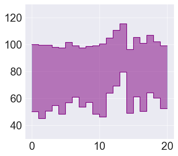
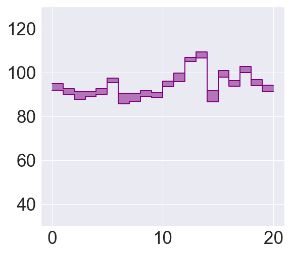
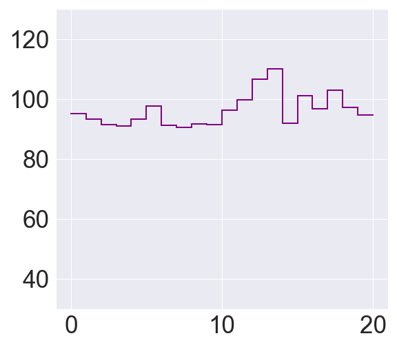
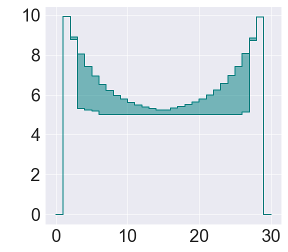
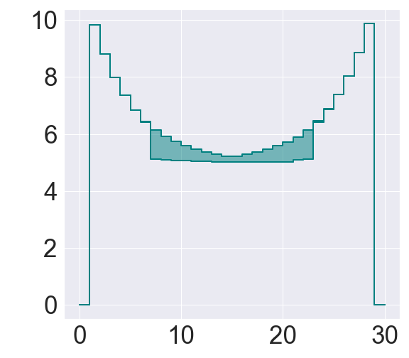
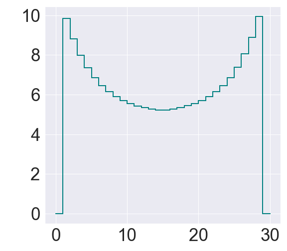
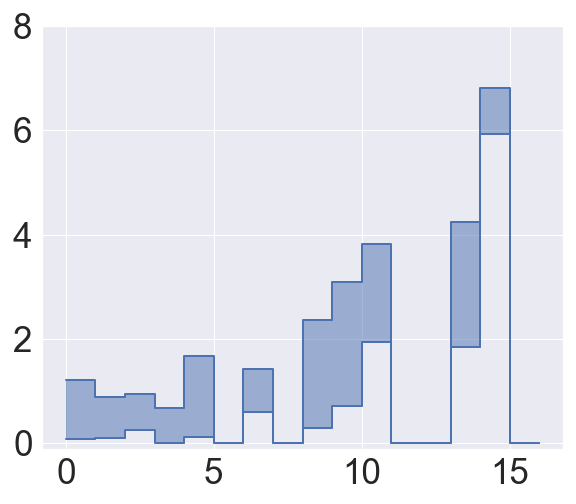
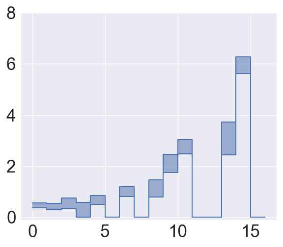
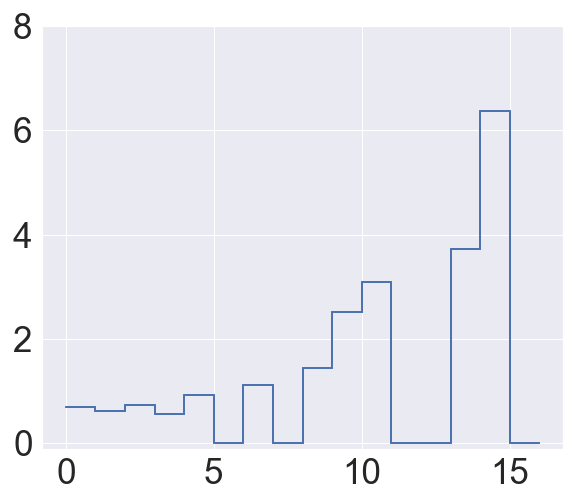
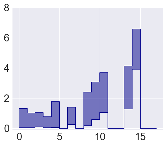
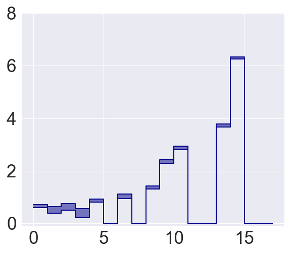
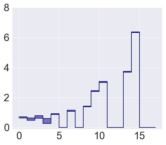
Figure 1: The difference between $V^{\rm{up},\pi_{i}}(x)$ and $V^{\pi_{i}}(x)$. X-axis represents states in a discrete environment for all pictures. Each group of three pictures of the same color demonstrates the process of learning the policy from the first iteration to the last. First row: Evaluation of the policies during the process of Value iteration for Garnet (left) and Chain environments (right). The policies are obtained greedily from $Q_{i}(x,a)$ function at the i-th step. Second row: Comparison of Value iteration process (left) and Reinforce algorithm (right) during learning for Frozen Lake.

Continuous state-space MDPs

We consider the AI Gym CartPole and Acrobot environments (Brockman et al. (2016)). Their descriptions can be found in Appendix 9. For CartPole we evaluate A2C algorithm policy $\pi_{1}$ (Mnih et al. (2016)), linear deterministic policy (LD) $\pi_{2}$ described in  9 and random uniform policy $\pi_{3}$. Figure 2 (left) indicates superior quality of $\pi_{2}$, sort of instability introduced by A2C training in $\pi_{1}$ and low quality of $\pi_{3}$. We also evaluated a policy for Acrobot given by A2C as well as a policy from Dueling DQN (Wang et al. (2016)) (Fig. 2 (right)). From the plots we can conclude that the both policies are good, but far from optimal.

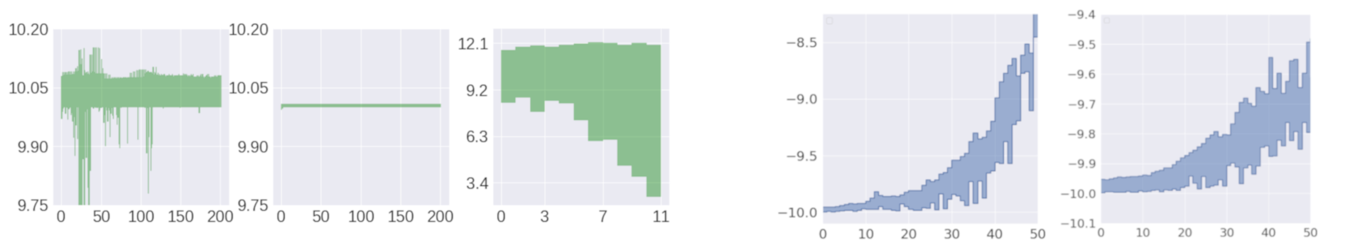
Figure 2: Upper and lower bounds of the three different policies. Left: For CartPole $\pi_{1}$, $\pi_{2}$, $\pi_{3}$ policies, respectively. For horizontal axis we sample single trajectory according to the policy. Right: For Acrobot Dueling DQN and A2C policies, respectively. We evaluated the bounds for 50 first states of the trajectory for each algorithm.

7 Conclusion and future work

In this work we propose a new approach towards model-free evaluation of the agent’s policies in RL, based on upper solutions to the Bellman optimality equation (1). To the best of our knowledge, the UVIP is the first procedure which allows to construct the non-asymptotic confidence intervals for the optimal value function $V^{\star}$ based on the value function corresponding to an arbitrary policy $\pi$. In our analysis we consider only infinite-horizon MDPs and assume that sampling from the conditional distribution ${\rm P}^{a}(\cdot|x)$ is feasible for any $x\in\mathsf{X}$ and $a\in\mathsf{A}.$ A promising future research direction is to generalize UVIP to the case of finite-horizon MDPs combining it with the idea of Real-time dynamic programming (see Efroni et al. (2019)). Moreover, the plain Monte Carlo estimates are not necessarily the most efficient way to estimate the outer expectation in Algorithm $1$. Other stochastic approximation techniques could also be applied to approximate the solution of (2).

8 Proof of the main results

Throughout this section we will use additional notations. Let $\psi_{2}(x)=e^{x^{2}}-1$, $x\in\mathbb{R}$. For r.v. $\eta$ we denote $\|\eta\|_{\psi_{2}}\doteq\inf\{t>0:\mathsf{E}\left[\exp\{\eta^{2}/t^{2}\}\right]\leq 2\}$ the Orlicz 2-norm. We say that $\eta$ is a sub-Gaussian random variable if $\|\eta\|_{\psi_{2}}<\infty$. In particular, this implies that for some constants $C,c>0$, $\mathrm{P}(|\eta|\geq t)\leq 2\exp\{-ct^{2}/\|\eta\|_{\psi_{2}}^{2}\}$ and $\mathsf{E}^{1/p}[|\eta|^{p}]\leq C\sqrt{p}\|\eta\|_{\psi_{2}}$ for all $p\geq 1$. Consider a random process $(X_{t})_{t\in T}$ on a metric space $(T,\mathsf{d})$. We say that the process has sub-Gaussian increments if there exists $K\geq 0$ such that

$$\|X_{t}-X_{s}\|_{\psi_{2}}\leq K\mathsf{d}(t,s),\quad\forall t,s\in T.$$

We start from the following proposition.

Proposition 8.1.

Under A1 – A4 for any $M\in\mathbb{N}$ and $p\geq 1$

$$\mathsf{E}^{1/p}\Bigl{[}\Bigl{\|}\frac{1}{M}\sum_{l=1}^{M}[V^{\pi}(\psi(\cdot,\cdot,\xi_{l}))-\mathsf{E}V^{\pi}(\psi(\cdot,\cdot,\xi_{l}))]\Bigr{\|}_{\mathsf{X}\times\mathcal{A}}^{p}\Bigr{]}\lesssim\frac{L_{\pi}I_{\mathcal{D}}+\{L_{\pi}\mathsf{D}+R_{\max}/(1-\gamma)\}\sqrt{p}}{\sqrt{M}}.$$

Proof.

We apply the empirical process methods. To simplify notations we denote

$$Z(x,a)=\frac{1}{\sqrt{M}}\sum_{\ell=1}^{M}[V^{\pi}(\psi(x,a,\xi_{\ell}))-\mathsf{E}V^{\pi}(\psi(x,a,\xi_{\ell}))],\,(x,a)\in\mathsf{X}\times\mathsf{A},$$

that is, $Z(x,a)$ is a random process on the metric space $(\mathsf{X}\times\mathsf{A},\rho)$. Below we show that the process $Z(x,a)$ has sub-Gaussian increments. In order to show it, let us introduce for $\ell\in[M]$

$$Z_{\ell}\doteq[V^{\pi}(\psi(x,a,\xi_{l}))-\mathsf{E}V^{\pi}(\psi(x,a,\xi_{l}))]-[V^{\pi}(\psi(x^{\prime},a^{\prime},\xi_{l}))-\mathsf{E}V^{\pi}(\psi(x^{\prime},a^{\prime},\xi_{l}))]\,.$$

Clearly, by A4,

$$\|Z_{\ell}\|_{\psi_{2}}\lesssim L_{\pi}\rho((x,a),(x^{\prime},a^{\prime}))\,,$$

that is, $Z_{\ell}$ is a sub-Gaussian r.v. for any $\ell\in[M]$. Since $Z(x,a)-Z(x^{\prime},a^{\prime})=M^{-1/2}\sum_{\ell=1}^{M}Z_{\ell}$ is a sum of independent sub-Gaussian r.v, we may apply [Vershynin, 2018, Proposition 2.6.1 and Eq. (2.16)]) to obtain that $Z(x,a)$ has sub-Gaussian increments with parameter $K\asymp L_{\pi}$. Fix some $(x_{0},a_{0})\in\mathsf{X}\times\mathsf{A}$. By the triangular inequality,

$$\sup_{(x,a)\in\mathsf{X}\times\mathsf{A}}|Z(x,a)|\leq\sup_{(x,a),(x^{\prime},a^{\prime})\in\mathsf{X}\times\mathsf{A}}|Z(x,a)-Z(x^{\prime},a^{\prime})|+Z(x_{0},a_{0}).$$ (15)

By the Dudley integral inequality, e.g. [Vershynin, 2018, Theorem 8.1.6], for any $\delta\in(0,1)$,

$$\sup_{(x,a),(x^{\prime},a^{\prime})\in\mathsf{X}\times\mathsf{A}}|Z(x,a)-Z(x^{\prime},a^{\prime})|\lesssim L_{\pi}\bigl{[}I_{\mathcal{D}}+\mathsf{D}\sqrt{\log(2/\delta)}\bigr{]}\,.$$

holds with probability at least $1-\delta$. Again, under A3, $Z(x_{0},a_{0})$ is a sum of i.i.d. bounded centered random variables with $\psi_{2}$-norm bounded by $R_{\max}/(1-\gamma)$. Hence, applying Hoeffding’s inequality, e.g. [Vershynin, 2018, Theorem 2.6.2.], for any $\delta\in(0,1)$,

$$|Z(x_{0},a_{0})|\lesssim R_{\max}\sqrt{\log(1/\delta)}/(1-\gamma)$$

holds with probability $1-\delta$. The last two inequalities and (15) imply the statement. ∎

8.1 Proof of Theorem 5.1

Fix $p\geq 2$ and denote for any $k\in\mathbb{N}$, ${\mathcal{M}}_{k}\doteq\mathsf{E}^{1/p}[\|\widehat{V}_{k}^{{\rm{up}}}-V^{{\rm*}}\|_{\mathsf{X}}^{p}]$. For any $x\in\mathsf{X}$, we introduce

$$\widetilde{V}_{k+1}^{{\rm{up},\pi}}(x)=\frac{1}{M_{2}}\sum_{j=M_{1}+1}^{M_{1}+M_{2}}\max_{a}\left\{r^{a}(x)+\gamma\Bigl{(}\widehat{V}_{k}^{{\rm{up}}}(Y_{j}^{x,a})-V^{\pi}(Y_{j}^{x,a})+\frac{1}{M_{1}}\sum_{\ell=1}^{M_{1}}V^{\pi}(Y_{\ell}^{x,a})\Bigr{)}\right\}$$

Recall that $Y_{j}^{x,a}=\psi(x,a,\xi_{k,j}),j\in[M_{1}+M_{2}]$ for independent random variables $(\xi_{k,j})$, thus we can write

$$\widetilde{V}_{k+1}^{{\rm{up},\pi}}(x)=\frac{1}{M_{2}}\sum_{j=M_{1}+1}^{M_{1}+M_{2}}R_{k}^{x}(\xi_{k,j};\xi_{k,1},\ldots,\xi_{k,M_{1}})\,.$$ (16)

We first calculate $L_{k+1}\doteq\mathrm{Lip}_{\rho}(\widetilde{V}_{k+1}^{{\rm{up},\pi}})$ for any $k\in\mathbb{N}$. Since under A4, $\mathrm{Lip}_{\rho}((V^{\pi}\circ\psi)(\cdot,\cdot,\xi))\leq L_{\pi}$, and using (16),

$$L_{k+1}\leq L_{\max}+\gamma(L_{k}L_{\psi}+2L_{\pi})\,.$$ (17)

Expanding (17) and using the assumptions of Theorem 5.1, we obtain

$$L_{k+1}\leq\frac{L_{\max}+2\gamma L_{\pi}}{1-\gamma L_{\psi}}+(\gamma L_{\psi})^{k}L_{0}\,,\quad k\in\mathbb{N}\,.$$

Using that $\gamma L_{\psi}<1$, the maximal Lipshitz constant of $\widetilde{V}_{k}^{{\rm{up},\pi}}(x),k\in\mathbb{N}$ is uniformly bounded by

$$L_{V}=\frac{L_{\max}+2\gamma L_{\pi}}{1-\gamma L_{\psi}}+L_{0}\,.$$ (18)

Using (16) and  (4), for any $x\in\mathsf{X}$ and $j=M_{1}+1,\ldots,M_{1}+M_{2}$.

$$\begin{split}&\mathsf{E}^{1/p}[|R_{k}^{x}(\xi_{k,j};\xi_{k,1},\ldots,\xi_{k,M_{1}})-V^{*}(x)|^{p}]\leq\\ &\mathsf{E}^{1/p}\left[\left|\max_{a}\left\{r^{a}(x)+\gamma\Bigl{(}\widehat{V}_{k}^{{\rm{up}}}(Y_{j}^{x,a})-V^{\pi}(Y_{j}^{x,a})+M_{1}^{-1}\sum\nolimits_{\ell=1}^{M_{1}}V^{\pi}(Y_{\ell}^{x,a})\Bigr{)}\right\}\right.\right.-\\ &\qquad\left.\left.\max_{a}\left\{r^{a}(x)+\gamma(V^{\star}(Y^{x,a})-V^{\star}(Y^{x,a})+{\rm P}^{a}V^{\star}(x)\right\}\right|^{p}\right]\end{split}$$

Hence, with the Minkowski inequality and $|{\rm P}^{a}V^{\star}(x)-\mathsf{E}V^{\pi}(\psi(x,a,\cdot))|\leq\|V^{\pi}-V^{*}\|_{\mathsf{X}}$, we get

$$\begin{split}&\mathsf{E}^{1/p}[|R_{k}^{x}(\xi_{k,j};\xi_{k,1},\ldots,\xi_{k,M_{1}})-V^{*}(x)|^{p}]\leq\gamma{\mathcal{M}}_{k}+2\gamma\left\|V^{\pi}-V^{{\rm*}}\right\|_{\mathsf{X}}\\ &\qquad\qquad\qquad+\gamma\mathsf{E}^{1/p}\Bigl{[}\Bigl{\|}M_{1}^{-1}\sum\nolimits_{\ell=1}^{M_{1}}[V^{\pi}(\psi(\cdot,\cdot,\xi_{k,\ell}))-\mathsf{E}V^{\pi}(\psi(\cdot,\cdot,\xi_{k,\ell}))]\Bigr{\|}_{\mathsf{X}\times\mathcal{A}}^{p}\Bigr{]}\end{split}$$ (19)

To analyze the last term we use the empirical process methods. By Proposition 8.1, we get

$$\mathsf{E}^{1/p}\Bigl{[}\Bigl{\|}\frac{1}{M_{1}}\sum_{\ell=1}^{M_{1}}[V^{\pi}(\psi(\cdot,\cdot,\xi_{k,\ell}))-\mathsf{E}V^{\pi}(\psi(\cdot,\cdot,\xi_{k,\ell}))]\Bigr{\|}_{\mathsf{X}\times\mathcal{A}}^{p}\Bigr{]}\lesssim\frac{L_{\pi}I_{\mathcal{D}}+\{L_{\pi}\mathsf{D}+R_{\max}/(1-\gamma)\}\sqrt{p}}{\sqrt{M_{1}}}.$$

Furthermore, with (7) we construct Lipshitz interpolant $\widehat{V}_{k+1}^{{\rm{up}}}$, such that

$$|\widehat{V}_{k+1}^{{\rm{up}}}(x)-\widetilde{V}_{k+1}^{{\rm{up},\pi}}(x)| \lesssim L_{k+1}\rho(\mathsf{X}_{N},\mathsf{X})\,.$$

Combining the above estimates, we get

$${\mathcal{M}}_{k+1} \lesssim \gamma{\mathcal{M}}_{k}+\gamma\left\|V^{\pi}-V^{{\rm*}}\right\|_{\mathsf{X}}+\gamma\frac{L_{\pi}I_{\mathcal{D}}+\{L_{\pi}\mathsf{D}+R_{\max}/(1-\gamma)\}\sqrt{p}}{\sqrt{M_{1}}}+L_{k+1}\rho(\mathsf{X}_{N},\mathsf{X})\,.$$

Iterating this inequality,

$$\mathsf{E}^{1/p}[\|\widehat{V}_{k}^{{\rm{up}}}-V^{{\rm*}}\|_{\mathsf{X}}^{p}]\lesssim\gamma^{k}\bigl{\|}\widehat{V}_{0}^{{\rm{up}}}-V^{{\rm*}}\bigr{\|}_{\mathsf{X}}+\frac{\gamma}{1-\gamma}\left\|V^{\pi}-V^{{\rm*}}\right\|_{\mathsf{X}}+\\ \frac{\gamma L_{\pi}I_{\mathcal{D}}+\gamma\{L_{\pi}\mathsf{D}+R_{\max}/(1-\gamma)\}\sqrt{p}}{\sqrt{M_{1}}(1-\gamma)}+\frac{L_{V}}{1-\gamma}\rho(\mathsf{X}_{N},\mathsf{X})\,.$$ (20)

Applying Markov’s inequality with $p\asymp\log{(1/\delta)}$, we get that for any $k\in\mathbb{N}$ and $\delta\in(0,1)$,

$$\begin{split}&\|\widehat{V}_{k}^{{\rm{up}}}-V^{{\rm*}}\|_{\mathsf{X}}\lesssim\gamma^{k}\bigl{\|}\widehat{V}_{0}^{{\rm{up}}}-V^{{\rm*}}\bigr{\|}_{\mathsf{X}}+\frac{\gamma}{1-\gamma}\left\|V^{\pi}-V^{{\rm*}}\right\|_{\mathsf{X}}+\\ &\quad\frac{\gamma L_{\pi}I_{\mathcal{D}}+\gamma\{L_{\pi}\mathsf{D}+R_{\max}/(1-\gamma)\}\sqrt{\log(1/\delta)}}{\sqrt{M_{1}}(1-\gamma)}+\frac{L_{V}}{1-\gamma}\rho(\mathsf{X}_{N},\mathsf{X})\,.\end{split}$$ (21)

holds with probability at least $1-\delta$, where the constant $L_{V}$ is given in (18). This yields the statement of the theorem.

8.2 Proof of Corollary 5.1 and Corollary 5.2

Proof of Corollary 5.1.

Consider $\rho((x,a),(x^{\prime},a^{\prime}))=\mathbbm{1}_{\{(x,a)\neq(x^{\prime},a^{\prime})\}}$ and $\mathsf{X}_{N}=\mathsf{X}$, that is, we bypass the approximation step. Then $\mathsf{D}=1$, $I_{\mathcal{D}}\lesssim\sqrt{\log(|\mathsf{X}||\mathsf{A}|)}$, $\rho(\mathsf{X}_{N},\mathsf{X})=0$, and $r^{a}(\cdot)$ is Lipshitz w.r.t. $\rho_{\mathsf{X}}$ with $L_{\max}\leq R_{\max}$. Moreover, one can take $L_{\psi}=1$ and $L_{\pi}=R_{\max}/(1-\gamma)$ in Assumption A4. Hence, A1 – A4 are valid and one may apply Theorem 5.1. Bound (21) in this case writes as

$$\|\widehat{V}_{k}^{{\rm{up}}}-V^{{\rm*}}\|_{\mathsf{X}}\lesssim\gamma^{k}\bigl{\|}\widehat{V}_{0}^{{\rm{up}}}-V^{{\rm*}}\bigr{\|}_{\mathsf{X}}+\frac{\gamma}{1-\gamma}\left\|V^{\pi}-V^{{\rm*}}\right\|_{\mathsf{X}}+\\ \frac{\gamma R_{\max}(\sqrt{\log(|\mathsf{X}||\mathsf{A}|)}+2)\sqrt{\log{(1/\delta)}}}{\sqrt{M_{1}}(1-\gamma)^{2}}\,.$$ (22)

∎

Proof of Corollary 5.2.

It is easy to see that $\mathsf{D}\leq\sqrt{{d_{\mathsf{X}}}}+1$, $I_{\mathcal{D}}\lesssim\sqrt{{d_{\mathsf{X}}}\log|\mathsf{A}|}+\sqrt{{d_{\mathsf{X}}}\log{d_{\mathsf{X}}}}$. Proposition 8.2 implies that for any $\delta\in(0,1)$, $\rho(\mathsf{X}_{N},\mathsf{X})\lesssim\sqrt{{d_{\mathsf{X}}}}\left(N^{-1}\log(1/\delta)\log N\right)^{1/{d_{\mathsf{X}}}}$. Substituting into (21), we obtain

$$\|\widehat{V}_{k}^{{\rm{up}}}-V^{{\rm*}}\|_{\mathsf{X}}\lesssim\gamma^{k}\bigl{\|}\widehat{V}_{0}^{{\rm{up}}}-V^{{\rm*}}\bigr{\|}_{\mathsf{X}}+\frac{\gamma}{1-\gamma}\left\|V^{\pi}-V^{{\rm*}}\right\|_{\mathsf{X}}+\frac{L_{V}\sqrt{{d_{\mathsf{X}}}}\left(N^{-1}\log(1/\delta)\log N\right)^{1/{d_{\mathsf{X}}}}}{1-\gamma}\\ +\frac{\gamma L_{\pi}(\sqrt{{d_{\mathsf{X}}}\log|\mathsf{A}|}+\sqrt{{d_{\mathsf{X}}}\log{d_{\mathsf{X}}}})+\gamma\{L_{\pi}\sqrt{{d_{\mathsf{X}}}}+R_{\max}/(1-\gamma)\}\sqrt{\log(1/\delta)}}{\sqrt{M_{1}}(1-\gamma)}\,,$$ (23)

where $L_{V}$ is given in (18). ∎

8.3 Proof of Theorem 5.2

We use definition of $\widetilde{V}_{k+1}^{{\rm{up},\pi}}(x)$ and $R_{k}^{x}(\xi_{k,j};\xi_{k,1},\ldots,\xi_{k,M_{1}})$ from Theorem 5.1. To simplify notations we denote $\boldsymbol{\xi}_{k,M_{1}}=(\xi_{k,1},\ldots,\xi_{k,M_{1}})$ and $\boldsymbol{\xi}_{k,M_{2}}=(\xi_{k,M_{1}+1},\ldots,\xi_{k,M_{1}+M_{2}})$. In these notations $\boldsymbol{\xi}_{k}=(\boldsymbol{\xi}_{k,M_{1}},\boldsymbol{\xi}_{k,M_{2}})$. Recall that, by the construction, $\widetilde{V}_{k+1}^{{\rm{up},\pi}}(x)$ can be evaluated only at the points $x\in\{\mathsf{x}_{1},\dots,\mathsf{x}_{N}\}$. By the definition,

$$\widehat{V}_{k+1}^{{\rm{up}}}(x)=\min_{\ell\in[N]}\bigl{\{}\widetilde{V}_{k+1}^{{\rm{up},\pi}}(\mathsf{x}_{\ell})+L_{V}\rho_{\mathsf{X}}(\mathsf{x}_{\ell},x)\bigr{\}}\,,$$ (24)

where the constant $L_{V}$ is given in (18). We rewrite $\widetilde{V}_{k+1}^{{\rm{up},\pi}}(x)$ as follows

$$\widetilde{V}_{k+1}^{{\rm{up},\pi}}(x) = \frac{1}{M_{2}}\sum_{j=M_{1}+1}^{M_{1}+M_{2}}\{R_{k}^{x}(\xi_{k,j};\boldsymbol{\xi}_{k,M_{1}})-\mathsf{E}[R_{k}^{x}(\xi_{k,j};\boldsymbol{\xi}_{k,M_{1}})]\}$$

$$+ \mathsf{E}[R_{k}^{x}(\xi;\boldsymbol{\xi}_{k,M_{1}})]=:T_{k}^{x}(\boldsymbol{\xi}_{k})+\mathsf{E}[R_{k}^{x}(\xi;\boldsymbol{\xi}_{k,M_{1}})],$$

where $\xi$ is an i.i.d. copy of $\xi_{k,j}$. Conditioned on $\overline{\mathcal{G}}_{k}\doteq\mathcal{G}_{k-1}\cup\sigma\{\boldsymbol{\xi}_{k,M_{1}}\}$, $T_{k}^{x}(\boldsymbol{\xi}_{k,M_{1}},\boldsymbol{\xi}_{k,M_{2}})$ is the sum of i.i.d. centered random variables. In what follows we will often omit the arguments $\boldsymbol{\xi}_{k,M_{1}}$ and/or $\boldsymbol{\xi}_{k,M_{2}}$ from the notations of functions $T_{k}^{x}$. Using representation (24),

$$\operatorname{Var}[\widehat{V}_{k+1}^{{\rm{up}}}(x)] =\operatorname{Var}\left[\min_{\ell\in[N]}\bigl{\{}\widetilde{V}_{k+1}^{{\rm{up},\pi}}(\mathsf{x}_{\ell})+L_{V}\rho_{\mathsf{X}}(\mathsf{x}_{\ell},x)\bigr{\}}\right]$$

$$\leq\mathsf{E}\left[\left(\min_{\ell\in[N]}\bigl{\{}\widetilde{V}_{k+1}^{{\rm{up},\pi}}(\mathsf{x}_{\ell})+L_{V}\rho_{\mathsf{X}}(\mathsf{x}_{\ell},x)\bigr{\}}-\min_{\ell\in[N]}\bigl{\{}\mathsf{E}[R_{k}^{x}(\xi;\boldsymbol{\xi}_{k,M_{1}})]+L_{V}\rho_{\mathsf{X}}(\mathsf{x}_{\ell},x)\bigr{\}}\right)^{2}\right]\,.$$

Hence, from the previous inequality and the definition of $\widetilde{V}_{k+1}^{{\rm{up},\pi}}(x)$,

$$\operatorname{Var}[\widehat{V}_{k+1}^{{\rm{up}}}(x)]\leq\mathsf{E}[\sup_{\ell\in[N]}|T_{k}^{\mathsf{x}_{\ell}}(\boldsymbol{\xi}_{k,M_{1}},\boldsymbol{\xi}_{k,M_{2}})|^{2}]\leq\mathsf{E}[\sup_{x\in\mathsf{X}}|T_{k}^{x}(\boldsymbol{\xi}_{k,M_{1}},\boldsymbol{\xi}_{k,M_{2}})|^{2}].$$

To estimate the r.h.s. of the previous inequality we again apply the empirical process method. We first note that for any $x,x^{\prime}\in\mathsf{X}$,

$$\sup_{\boldsymbol{\xi}\in\Xi^{M_{1}+M_{2}}}|T_{k}^{x}(\boldsymbol{\xi})-T_{k}^{x^{\prime}}(\boldsymbol{\xi})|\leq L_{T}\rho_{\mathsf{X}}(x,x^{\prime}),$$ (25)

where

$$L_{T}=L_{\max}+\gamma(L_{V}+2L_{\pi})\,.$$ (26)

Now we freeze the coordinates $\boldsymbol{\xi}_{M_{1}}$ and consider $T_{k}^{x}(\boldsymbol{\xi}_{M_{1}},\cdot)$ as a function on $\Xi^{M_{2}}$, parametrized by $x\in\mathsf{X}$. Introduce a parametric class of functions

$$\mathcal{T}_{k,\boldsymbol{\xi}_{M_{1}}}\doteq\bigl{\{}T_{k}^{x}(\boldsymbol{\xi}_{M_{1}},\cdot):\Xi^{M_{2}}\to\mathbb{R},x\in\mathsf{X}\bigr{\}}\,.$$

For notational simplicity we will omit dependencies on $k$ and $\boldsymbol{\xi}_{M_{1}}$, and simply write $T^{x}(\cdot)=T_{k}^{x}(\boldsymbol{\xi}_{M_{1}},\cdot)$. Note that the functions in $\mathcal{T}_{k,\boldsymbol{\xi}_{M_{1}}}$ are Lipshitz w.r.t. the uniform metric

$$\rho_{\mathcal{T}_{k,\boldsymbol{\xi}_{M_{1}}}}(T^{x}(\cdot),T^{x^{\prime}}(\cdot))=\sup_{\boldsymbol{\xi}_{M_{2}}\in\Xi^{M_{2}}}|T^{x}(\boldsymbol{\xi}_{M_{2}})-T^{x^{\prime}}(\boldsymbol{\xi}_{M_{2}})|,\quad T^{x}(\cdot),\,T^{x^{\prime}}(\cdot)\in\mathcal{T}_{k,\boldsymbol{\xi}_{M_{1}}}\,.$$

To estimate $\operatorname{diam}(\mathcal{T}_{k,\boldsymbol{\xi}_{M_{1}}})$ we proceed as follows. Denote $\tilde{R}_{k}^{x}(\xi;\boldsymbol{\xi}_{k,M_{1}})=R_{k}^{x}(\xi;\boldsymbol{\xi}_{k,M_{1}})-\mathsf{E}\left[R_{k}^{x}(\xi;\boldsymbol{\xi}_{k,M_{1}})\right]$. Using (19), we get an upper bound

$$\begin{split}&\left|\tilde{R}_{k}^{x}(\xi;\boldsymbol{\xi}_{k,M_{1}})\right|\lesssim\gamma\|\widehat{V}_{k}^{{\rm{up}}}-V^{{\rm*}}\|_{\mathsf{X}}+2\gamma\left\|V^{\pi}-V^{{\rm*}}\right\|_{\mathsf{X}}+\\ &\qquad\qquad\gamma\Bigl{\|}M_{1}^{-1}\sum_{l=1}^{M_{1}}[V^{\pi}(\psi(\cdot,\cdot,\xi_{k,l}))-\mathsf{E}V^{\pi}(\psi(\cdot,\cdot,\xi_{k,l}))]\Bigr{\|}_{\mathsf{X}\times\mathcal{A}}.\end{split}$$ (27)

We denote the r.h.s. of this inequality by $R_{k}^{\star}$. Clearly, $R_{k}^{\star}$ is $\overline{\mathcal{G}}_{k}$ – measurable function (recall that $\overline{\mathcal{G}}_{k}=\mathcal{G}_{k-1}\cup\sigma\{\boldsymbol{\xi}_{k,M_{1}}\}$). We may conclude that $\operatorname{diam}(\mathcal{T}_{k,\boldsymbol{\xi}_{M_{1}}})\leq 2R_{k}^{\star}$. Furthermore, by (25) its covering covering number can be bounded as

$$\mathcal{N}(\mathcal{T}_{k,\boldsymbol{\xi}_{M_{1}}},\rho_{\mathcal{T}},\varepsilon)\leq\mathcal{N}(\mathsf{X}\times\mathsf{A},\rho,\varepsilon/L_{T}).$$

It is also easy to check that $\bigl{(}T^{x}(\boldsymbol{\xi}_{k,M_{2}})\bigr{)},T^{x}\in\mathcal{T}_{k,\boldsymbol{\xi}_{M_{1}}}$ is a sub-Gaussian process on $(\mathcal{T}_{k,\boldsymbol{\xi}_{M_{1}}},\rho_{T})$ with

$$\|T^{x}-T^{x^{\prime}}\|_{\psi_{2}}\lesssim\rho_{\mathcal{T}}(T^{x},T^{x^{\prime}}).$$

Applying the tower property we get

$$\mathsf{E}[\sup_{x\in\mathsf{X}}|T_{k}^{x}(\boldsymbol{\xi}_{k,M_{2}})|^{2}]\leq\mathsf{E}[\mathsf{E}[\sup_{x\in\mathsf{X}}|T_{k}^{x}(\boldsymbol{\xi}_{k,M_{2}})|^{2}|\overline{\mathcal{G}}_{k}]]$$

Using the Dudley integral inequality, e.g. [Vershynin, 2018, Theorem 8.1.6] and assumption A5,

$$\mathsf{E}[\sup_{x\in\mathsf{X}}|T_{k}^{x}(\boldsymbol{\xi}_{k,M_{1}},\boldsymbol{\xi}_{k,M_{2}})|^{2}|\overline{\mathcal{G}}_{k}] = \mathsf{E}[\sup_{T^{x}\in\mathcal{T}_{k,\boldsymbol{\xi}_{M_{1}}}}|T^{x}(\boldsymbol{\xi}_{k,M_{2}})|^{2}|\overline{\mathcal{G}}_{k}]$$

$$\lesssim \mathsf{E}[|T^{x_{0}}(\boldsymbol{\xi}_{k,M_{2}})|^{2}|\overline{\mathcal{G}}_{k}]$$

$$+ \frac{1}{M_{2}}\Bigl{\{}L_{T}\sqrt{C_{\mathsf{X},\mathsf{A}}}\int_{0}^{2R_{k}^{\star}/L_{T}}\sqrt{\log(1+1/\varepsilon)}\mathrm{d}\varepsilon+R_{k}^{\star}\Bigr{\}}^{2},$$

where $x_{0}\in\mathsf{X}$ is some fixed point. To estimate the first term in the r.h.s. of the previous inequality we apply Hoeffding’s inequality, e.g. [Vershynin, 2018, Theorem]. We obtain

$$\mathsf{E}[|T^{x_{0}}(\boldsymbol{\xi}_{k,M_{2}})|^{2}|\overline{\mathcal{G}}_{k}]\lesssim\frac{(R_{k}^{\star})^{2}}{M_{2}}.$$

Applying Proposition 8.3 we get

$$\int_{0}^{2R_{k}^{\star}/L_{T}}\sqrt{\log(1+1/\varepsilon)}\mathrm{d}\varepsilon\lesssim(R_{k}^{\star}\sqrt{\log(1+1/R_{k}^{\star})}+R_{k}^{\star})/L_{T}.$$

The last two inequalities imply

$$\mathsf{E}[\sup_{x\in\mathsf{X}}|T_{k}^{x}(\boldsymbol{\xi}_{k,M_{2}})|^{2}|\overline{\mathcal{G}}_{k}]\lesssim C_{\mathsf{X},\mathsf{A}}\frac{(R_{k}^{\star})^{2}+(R_{k}^{\star})^{2}\log(1+1/R_{k}^{\star})}{M_{2}}.$$

Since for $x>0$ and $\varepsilon\in(0,1]$

$$\log(1+x)\leq\varepsilon^{-1}x^{\varepsilon},$$

we obtain

$$\mathsf{E}[\sup_{x\in\mathsf{X}}|T_{k}^{x}|^{2}]\lesssim C_{\mathsf{X},\mathsf{A}}\frac{\mathsf{E}[(R_{k}^{\star})^{2}]+\mathsf{E}[(R_{k}^{\star})^{2-\varepsilon}]/\varepsilon}{M_{2}}\,.$$

Using (27), we get for any $p\geq 1$

$$\begin{split}\mathsf{E}^{1/p}\bigl{[}(R_{k}^{\star})^{p}\bigr{]}&\leq\gamma\mathsf{E}^{1/p}\bigl{[}\|\widehat{V}_{k}^{{\rm{up}}}-V^{{\rm*}}\|^{p}_{\mathsf{X}}\bigr{]}+2\gamma\left\|V^{\pi}-V^{{\rm*}}\right\|_{\mathsf{X}}+\\ &\qquad\gamma\mathsf{E}^{1/p}\left[\Bigl{\|}M_{1}^{-1}\sum_{l=1}^{M_{1}}[V^{\pi}(\psi(\cdot,\cdot,\xi_{k,l}))-\mathsf{E}V^{\pi}(\psi(\cdot,\cdot,\xi_{k,l}))]\Bigr{\|}^{p}_{\mathsf{X}\times\mathcal{A}}\right].\end{split}$$

Thus, applying (20) and Proposition 8.1, for any $p\geq 1$,

$$\mathsf{E}^{1/p}\bigl{[}(R_{k}^{\star})^{p}\bigr{]}\leq 3\operatorname{C}_{0}\sigma_{k}\,.$$

Here the quantity $\sigma_{k}$ is defined in (11), and the constant $\operatorname{C}_{0}$ is given by

$$\operatorname{C}_{0}=\max\left\{\frac{\gamma L_{\pi}}{1-\gamma}+\frac{R_{\max}}{(1-\gamma)^{2}},\frac{L_{\max}+2\gamma L_{\pi}}{(1-\gamma L_{\psi})(1-\gamma)}+\frac{L_{0}}{1-\gamma},\frac{\gamma}{1-\gamma}\right\}\,.$$ (28)

This yields the final bound

$$\operatorname{Var}[\widehat{V}_{k+1}^{{\rm{up}}}(x)]\leq\mathsf{E}[\sup_{x\in\mathsf{X}}|T_{k}^{x}|^{2}]\leq 9C_{\mathsf{X},\mathsf{A}}\operatorname{C}_{0}^{2}\frac{\sigma_{k}^{2}+\sigma_{k}^{2-\varepsilon}/\varepsilon}{M_{2}}\doteq\operatorname{C}\frac{\sigma_{k}^{2}+\sigma_{k}^{2-\varepsilon}/\varepsilon}{M_{2}}\,.$$ (29)

Now the statement follows by the choice $\varepsilon=\log^{-1}(\mathrm{e}\vee\Delta_{k}^{-1})$.

8.4 Proof of Proposition 5.1

Applying (11) with $I_{\mathcal{D}}\lesssim\sqrt{\log{|\mathsf{X}||\mathsf{A}|}}$, $\mathsf{D}=1$, we obtain that

$$\sigma_{k}\lesssim\gamma^{k}\bigl{\|}\widehat{V}_{0}^{{\rm{up}}}-V^{{\rm*}}\bigr{\|}_{\mathsf{X}}+\left\|V^{\pi}-V^{{\rm*}}\right\|_{\mathsf{X}}+\frac{\gamma R_{\max}(\sqrt{\log(|\mathsf{X}||\mathsf{A}|)}+1)}{\sqrt{M_{1}}(1-\gamma)^{2}}.$$

Note that, under assumption A3, $\bigl{\|}V^{\star}\bigr{\|}_{\mathsf{X}}\leq R_{\max}(1-\gamma)^{-1}$. Hence, the previous bound implies $\sigma_{k}\lesssim\left\|V^{\pi}-V^{\star}\right\|_{\mathsf{X}}$, provided that $k$ and $M_{1}$ are large enough to guarantee

$$\gamma^{k-1}R_{\max}\leq\left\|V^{\pi}-V^{\star}\right\|_{\mathsf{X}},\quad R_{\max}(\sqrt{\log(|\mathsf{X}||\mathsf{A}|)}+1)M_{1}^{-1/2}(1-\gamma)^{-2}\leq\left\|V^{\pi}-V^{\star}\right\|_{\mathsf{X}}\,.$$

Thus, it is enough to choose

$$\begin{split}&k\geq\log{\left\|V^{\pi}-V^{\star}\right\|_{\mathsf{X}}}(\log{(1/\gamma)})^{-1}\,,\\ &M_{1}\geq R_{\max}^{2}(\sqrt{\log(|\mathsf{X}||\mathsf{A}|)}+1)^{2}((1-\gamma)^{2}\left\|V^{\pi}-V^{\star}\right\|_{\mathsf{X}})^{-2}\,.\end{split}$$ (30)

8.5 The covering radius radius of randomly distributed points over a cube

The following proposition is a particular case of the result [Reznikov and Saff, 2016, Theorem 2.1]. We repeat the arguments from that paper and give explicit expressions for the constants.

Proposition 8.2.

Let $\mathsf{X}=[0,1]^{d_{\mathsf{X}}}$ and $\mu$ be a uniform distribution on $\mathsf{X}$. Suppose that $\mathsf{X}_{N}=\{X_{1},\ldots,X_{N}\}$ is a set of $N$ points independently distributed over $\mathsf{X}$ w.r.t. $\mu$. Denote by $\rho(\mathsf{X}_{N},\mathsf{X})\doteq\max_{x\in\mathsf{X}}\min_{k\in[N]}|x-X_{k}|$ the covering radius of the set $\mathsf{X}_{N}$ w.r.t. $\mathsf{X}$. Then for any $p\geq 1$,

$$\mathsf{E}\left[\rho^{p}(\mathsf{X}_{N},\mathsf{X})\right]^{1/p}\lesssim\sqrt{{d_{\mathsf{X}}}}\left(\frac{p\log N}{N}\right)^{1/{d_{\mathsf{X}}}}.$$ (31)

Moreover, for any $\delta\in(0,1)$

$$\rho(\mathsf{X}_{N},\mathsf{X})\lesssim\sqrt{{d_{\mathsf{X}}}}\left(\frac{\log(1/\delta)\log N}{N}\right)^{1/{d_{\mathsf{X}}}}$$ (32)

holds with probability at least $1-\delta$.

Proof.

Let $\mathcal{E}_{n}=\mathcal{E}_{n}(\mathsf{X})$ be a maximal set of points such that for any $y,z\in\mathcal{E}_{n}$ we have $|y-z|\geq 1/n$. Then for any $x\in\mathsf{X}$ there exists a point $y\in\mathcal{E}_{n}$ such that $|x-y|\leq 1/n$. Denote by $B(x,r)$ a ball centred at $x\in\mathsf{X}$ of radius $r$ (w.r.t. $|\cdot|$) and

$$\Phi(r)=\frac{r^{d_{\mathsf{X}}}\pi^{{d_{\mathsf{X}}}/2}}{2^{d_{\mathsf{X}}}\Gamma({d_{\mathsf{X}}}/2+1)},\,r\in[0,\infty)$$

Since for any $x\in\mathsf{X}$, $\mu(B(x,r))\geq\Phi(r)$,

$$1=\mu(\mathsf{X})\geq\sum_{x\in\mathcal{E}_{n}}\mu(B(x,(1/3n)))\geq|\mathcal{E}_{n}|\Phi(1/(3n)).$$

Hence,

$$|\mathcal{E}_{n}|\leq\{\Phi(1/(3n))\}^{-1}.$$ (33)

Suppose that $\rho(\mathsf{X}_{N},\mathsf{X})>2/n$. Then there exists a point $y\in\mathsf{X}$ such that $\mathsf{X}_{N}\cap B(y,2/n)=\emptyset$. Choose a point $x\in\mathcal{E}_{n}$ such that $|x-y|<1/n$. Then $B(x,1/n)\subset B(y,2/n)$, and so the ball $B(x,1/n)$ doesn’t intersect $\mathsf{X}_{N}$. Hence, $\mathsf{X}_{N}\cap B(y,1/(3n))=\emptyset$. Therefore,

$$\mathrm{P}(\rho(\mathsf{X}_{N},\mathsf{X})>2/n) \leq \mathrm{P}(\exists x\in\mathcal{E}_{n}:\mathsf{X}_{N}\cap B(y,1/(3n))=\emptyset)\leq|\mathcal{E}_{n}|(1-\Phi(1/(3n))^{N}$$ (34)

$$\leq |\mathcal{E}_{n}|\mathrm{e}^{-N\Phi(1/(3n)}.$$ (35)

Let $1/(3n)=\Phi^{-1}(\alpha\log N/N)$ for some $\alpha>0$ to be chosen later. Then $\Phi(1/(3n))=\alpha\log N/N$. Inequalities (33) and (34) imply

$$\mathrm{P}(\rho(\mathsf{X}_{N},\mathsf{X})>2/n)\leq\frac{N^{1-\alpha}}{\alpha\log N}.$$ (36)

Let us fix any $p\geq 1$. Then

$$\mathsf{E}\left[\rho^{p}(\mathsf{X}_{N},\mathsf{X})\right]^{1/p}\leq\frac{2}{n}+\sqrt{{d_{\mathsf{X}}}}\left(\frac{N^{1-\alpha}}{\alpha\log N}\right)^{1/p}=6\Phi^{-1}(\alpha\log N/N)+\sqrt{{d_{\mathsf{X}}}}\left(\frac{N^{1-\alpha}}{\alpha\log N}\right)^{1/p}.$$ (37)

Since

$$\Phi^{-1}(r)=\frac{2}{\sqrt{\pi}}\Gamma^{1/{d_{\mathsf{X}}}}({d_{\mathsf{X}}}/2+1)r^{1/{d_{\mathsf{X}}}}\leq 2\sqrt{\mathrm{e}{d_{\mathsf{X}}}/\pi}(\mathrm{e}r)^{1/{d_{\mathsf{X}}}}$$

we get

$$\mathsf{E}\left[\rho^{p}(\mathsf{X}_{N},\mathsf{X})\right]^{1/p}\leq 12\sqrt{\mathrm{e}{d_{\mathsf{X}}}/\pi}\left(\frac{\alpha\mathrm{e}\log N}{N}\right)^{1/{d_{\mathsf{X}}}}+\sqrt{{d_{\mathsf{X}}}}\left(\frac{N^{1-\alpha}}{\alpha\log N}\right)^{1/p}.$$

It remains to take $\alpha=1+p/{d_{\mathsf{X}}}$ to obtain bound

$$\mathsf{E}\left[\rho^{p}(\mathsf{X}_{N},\mathsf{X})\right]^{1/p}\leq 48\sqrt{{d_{\mathsf{X}}}}\left(\frac{p\log N}{N}\right)^{1/{d_{\mathsf{X}}}}.$$

Hence, (31) follows. To prove (32) it remains to apply Markov’s inequality. ∎

8.6 Auxiliary results

Proposition 8.3.

For any $\Delta>0$,

$$\int_{0}^{\Delta}\sqrt{\log(1+1/x)}\mathrm{d}x\lesssim\Delta\sqrt{\log(1+1/\Delta)}+\Delta.$$

Proof.

Consider the case $\Delta<1$. In this case

$$\int_{0}^{\Delta}\sqrt{\log(1+1/x)}\mathrm{d}x = \int_{0}^{\Delta^{100}/2}\sqrt{\log(1+1/x)}\mathrm{d}x+\int_{\Delta^{100}/2}^{\Delta}\sqrt{\log(1+1/x)}\mathrm{d}x$$

$$\lesssim \int_{0}^{\Delta^{100}/2}x^{-1/2}\mathrm{d}x+\int_{\Delta^{100}/2}^{\Delta}\sqrt{\log(1+1/x)}\mathrm{d}x$$

$$\lesssim \Delta^{50}+(\Delta-\Delta^{100/2})\sqrt{\log(1+2/\Delta^{100})}$$

$$\lesssim \Delta\sqrt{\log(1+1/\Delta)}.$$

If $\Delta>1$,

$$\int_{0}^{\Delta}\sqrt{\log(1+1/x)}\mathrm{d}x = \int_{0}^{1}\sqrt{\log(1+1/x)}\mathrm{d}x+\int_{1}^{\Delta}\sqrt{\log(1+1/x)}\mathrm{d}x$$

$$\lesssim 2+(\Delta-1)\sqrt{\log 2}\lesssim\Delta.$$

∎

9 Experiment Setup

9.1 Environments description

Garnet

Garnet example is an MDP with randomly generated transition probability kernel ${\rm P}^{a}$ with finite $\mathsf{X}$ - state space and $\mathsf{A}$ - action space. This example is described with a tuple $\left\langle N_{S},N_{A},N_{B}\right\rangle$. The first two parameters specify the number of states and actions respectively. The last parameter is responsible for the number of states an agent can go to from state $x\in\mathsf{X}$ by performing action $a\in\mathsf{A}$. In our case we used $N_{S}=20,N_{A}=5,N_{B}=2,\gamma=0.9$. The reward matrix $r^{a}(x)$ is set according to the following principle: first, for all state-action pairs, the reward is set uniformly distributed on [0, 1]. Then the pairs are randomly chosen, for which the reward will be increased several times.

Frozen Lake

The agent moves in a grid world, where some squares of the lake are walkable, but others lead to the agent falling into the water, so the game restarts. Additionally, the ice is slippery, so the movement direction of the agent is uncertain and only partially depends on the chosen direction. The agent receives 10 points only for finding a path to a goal square, for falling into the hole it doesn’t receive anything. We used the built-in $4\times 4$ map and 4 actions for the agent to perform on each state if available (right, left, up and down). For this experiment we assume that the reward matrix $r^{a}(x)$ is known, $\gamma$-factor is set to be 0.9.

Chain

Chain is a finite MDP where agent can move only to 2 adjacent states performing 2 actions from each state (right and left). Every chain has two terminal states at the ends. For transition to the terminal states agent receives 10 points and episode ends, otherwise the reward is equal to +1. Also, there is p% noise in the system, that is the agent performs a uniformly-random action with probability p. For experiments with chains we set $\gamma$-factor to 0.8, to be sure that Pichard iterations converge.

CartPole

CartPole is an example of the environment with a finite action space and infinitely large state space. In this environment agent can push cart with pole on it to the left or right direction and the target is to hold the pole up as long as possible. Reward equals to 1 is gain every time until failing or the end of episode. In fact, CartPole hasn’t any specific stochastic dynamic, because transitions are deterministic according to actions, so for non degenerate case we should add some noise and we apply normally distributed random variable to the angle. LD(Linear Deterministic) policy can be expressed as I$\{3\cdot\theta+\dot{\theta}>0\}$, where $\theta$ is an angle between pole and normal to cart.

Acrobot

The environment consists of two joints, or two links. The torque is applied to the binding between the joints. The action space is discrete and consists of three kinds of torques: left, right and none. The state space is 6 dimensional, representing two angles (sine and cosine) characterizing the links position and the angles’ velocities. Each episode starts with the small perturbations of the parameters near the resting state having both of the joints in a downward position. The agents’ goal is to reach a given boundary from above in a minimum amount of time with its lower point of the link. At each timestep a robot has a reward equal to -1, and it gets 0 in a terminal state, when the boundary has been reached. Also to make the environment stochastic, a random uniform torque from $-1$ to $1$ is added to the force at each step.

9.2 Experimental setup

For the sake of completeness, we provide below hyperparameters for the experiments run in Section 6.

Table 1: Experimental hyperparameters

Environment		$M_{1}$	$M_{2}$	discount $\gamma$	$N$
Garnet		$3000$	$3000$	$0.9$	$-$
Frozen Lake		$1000$	$1000$	$0.9$	$-$
Chain		$1000$	$1000$	$0.8$	$-$
Cart Pole		$150$	$150$	$0.9$	$1500$
Acrobot		$150$	$100$	$0.9$	$4000$

9.3 Auxiliary algorithms

For the sake of completeness we provide here the Value iteration algorithm (Szepesvári [2010], Chapter 1), used in Section 6 for tabular environments.

Input: ${\rm P}^{a}$, $r$, $\varepsilon$

Result: $V^{\star}$

Initialize: $\forall x\in\mathsf{X},\ V^{\star}_{0}(x)=0$

$k=1$

while $\left\|V^{\star}_{k}-V^{\star}_{k-1}\right\|>\varepsilon$ do

       for $x\in\mathsf{X},\ a\in\mathsf{A}$ do

             $Q(x,a)=r^{a}(x)+\gamma\sum\limits_{y\in\mathsf{X}}{\rm P}^{a}(y|x)V^{\star}_{k-1}(y)$

             $V^{\star}_{k}(x)=\max\limits_{a\in\mathsf{A}}{Q(x,a)}$

       end for

      

      k = k + 1

end while

Algorithm 3 Value Iteration algorithm

References

- Antos et al. [2007] András Antos, Rémi Munos, and Csaba Szepesvári. Fitted q-iteration in continuous action-space mdps. 2007.
- Archibald et al. [1995] T. W. Archibald, K. I. M. McKinnon, and L. C. Thomas. On the generation of Markov Decision Processes. The Journal of the Operational Research Society, 46(3):354–361, 1995. ISSN 01605682, 14769360. URL http://www.jstor.org/stable/2584329.
- Azar et al. [2017] Mohammad Gheshlaghi Azar, Ian Osband, and Rémi Munos. Minimax regret bounds for reinforcement learning. 70:263–272, 06–11 Aug 2017. URL http://proceedings.mlr.press/v70/azar17a.html.
- Beliakov [2006] Gleb Beliakov. Interpolation of Lipschitz functions. Journal of computational and applied mathematics, 196(1):20–44, 2006.
- Belomestny and Schoenmakers [2018] Denis Belomestny and John Schoenmakers. Advanced Simulation-Based Methods for Optimal Stopping and Control: With Applications in Finance. Springer, 2018.
- Bertsekas and Shreve [1978] Dimitri P Bertsekas and Steven E Shreve. Stochastic optimal control, volume 139 of mathematics in science and engineering, 1978.
- Bertsekas and Tsitsiklis [1996] Dimitri P. Bertsekas and John N. Tsitsiklis. Neuro-Dynamic Programming. Athena Scientific, 1996. ISBN Athena Scientific. URL http://www.athenasc.com/ndpbook.html.
- Brockman et al. [2016] Greg Brockman, Vicki Cheung, Ludwig Pettersson, Jonas Schneider, John Schulman, Jie Tang, and Wojciech Zaremba. Openai gym, 2016.
- Ciosek and Whiteson [2020] Kamil Ciosek and Shimon Whiteson. Expected policy gradients for reinforcement learning. Journal of Machine Learning Research, 21(52):1–51, 2020. URL http://jmlr.org/papers/v21/18-012.html.
- Douc et al. [2018] Randal Douc, Eric Moulines, Pierre Priouret, and Philippe Soulier. Markov chains. Springer, 2018.
- Efroni et al. [2019] Yonathan Efroni, Nadav Merlis, Mohammad Ghavamzadeh, and Shie Mannor. Tight regret bounds for model-based reinforcement learning with greedy policies. In H. Wallach, H. Larochelle, A. Beygelzimer, F. d'Alché-Buc, E. Fox, and R. Garnett, editors, Advances in Neural Information Processing Systems, volume 32. Curran Associates, Inc., 2019. URL https://proceedings.neurips.cc/paper/2019/file/25caef3a545a1fff2ff4055484f0e758-Paper.pdf.
- Heess et al. [2015] Nicolas Heess, Gregory Wayne, David Silver, Timothy Lillicrap, Tom Erez, and Yuval Tassa. Learning continuous control policies by stochastic value gradients. 28, 2015. URL https://proceedings.neurips.cc/paper/2015/file/148510031349642de5ca0c544f31b2ef-Paper.pdf.
- Jaksch et al. [2010] Thomas Jaksch, Ronald Ortner, and Peter Auer. Near-optimal regret bounds for reinforcement learning. Journal of Machine Learning Research, 11(51):1563–1600, 2010. URL http://jmlr.org/papers/v11/jaksch10a.html.
- Jarner and Tweedie [2001] SF Jarner and RL Tweedie. Locally contracting iterated functions and stability of markov chains. Journal of applied probability, pages 494–507, 2001.
- Jin et al. [2018] Chi Jin, Zeyuan Allen-Zhu, Sebastien Bubeck, and Michael I Jordan. Is q-learning provably efficient? In S. Bengio, H. Wallach, H. Larochelle, K. Grauman, N. Cesa-Bianchi, and R. Garnett, editors, Advances in Neural Information Processing Systems, volume 31. Curran Associates, Inc., 2018. URL https://proceedings.neurips.cc/paper/2018/file/d3b1fb02964aa64e257f9f26a31f72cf-Paper.pdf.
- Liu et al. [2018] Hao Liu, Yihao Feng, Yi Mao, Dengyong Zhou, Jian Peng, and Qiang Liu. Action-dependent control variates for policy optimization via stein identity. February 2018. URL https://www.microsoft.com/en-us/research/publication/action-dependent-control-variates-policy-optimization-via-stein-identity/.
- Lyle et al. [2019] Clare Lyle, Marc G Bellemare, and Pablo Samuel Castro. A comparative analysis of expected and distributional reinforcement learning. In Proceedings of the AAAI Conference on Artificial Intelligence, volume 33, pages 4504–4511, 2019.
- Mnih et al. [2013] Volodymyr Mnih, Koray Kavukcuoglu, David Silver, Alex Graves, Ioannis Antonoglou, Daan Wierstra, and Martin Riedmiller. Playing Atari with Deep Reinforcement Learning. arXiv e-prints, art. arXiv:1312.5602, December 2013.
- Mnih et al. [2015] Volodymyr Mnih, Koray Kavukcuoglu, David Silver, Andrei A. Rusu, Joel Veness, Marc G. Bellemare, Alex Graves, Martin A. Riedmiller, Andreas Fidjeland, Georg Ostrovski, Stig Petersen, Charles Beattie, Amir Sadik, Ioannis Antonoglou, Helen King, Dharshan Kumaran, Daan Wierstra, Shane Legg, and Demis Hassabis. Human-level control through deep reinforcement learning. Nature, 518(7540):529–533, 2015.
- Mnih et al. [2016] Volodymyr Mnih, Adria Puigdomenech Badia, Mehdi Mirza, Alex Graves, Timothy Lillicrap, Tim Harley, David Silver, and Koray Kavukcuoglu. Asynchronous methods for deep reinforcement learning. In Maria Florina Balcan and Kilian Q. Weinberger, editors, Proceedings of The 33rd International Conference on Machine Learning, volume 48 of Proceedings of Machine Learning Research, pages 1928–1937, New York, New York, USA, 20–22 Jun 2016. PMLR. URL http://proceedings.mlr.press/v48/mniha16.html.
- Pires and Szepesvári [2016] Bernardo Ávila Pires and Csaba Szepesvári. Policy error bounds for model-based reinforcement learning with factored linear models. In Conference on Learning Theory, pages 121–151. PMLR, 2016.
- Puterman [2014] Martin L Puterman. Markov decision processes: discrete stochastic dynamic programming. John Wiley & Sons, 2014.
- Reznikov and Saff [2016] A. Reznikov and E. B. Saff. The covering radius of randomly distributed points on a manifold. Int. Math. Res. Not. IMRN, (19):6065–6094, 2016. ISSN 1073-7928. doi: 10.1093/imrn/rnv342. URL https://doi.org/10.1093/imrn/rnv342.
- Rogers [2007] L. Rogers. Pathwise stochastic optimal control. SIAM J. Control and Optimization, 46:1116–1132, 01 2007. doi: 10.1137/050642885.
- Rowland et al. [2020] Mark Rowland, Anna Harutyunyan, Hado van Hasselt, Diana Borsa, Tom Schaul, Rémi Munos, and Will Dabney. Conditional importance sampling for off-policy learning, 2020.
- Shar and Jiang [2020] Ibrahim El Shar and Daniel Jiang. Lookahead-bounded q-learning. In Hal Daumé III and Aarti Singh, editors, Proceedings of the 37th International Conference on Machine Learning, volume 119 of Proceedings of Machine Learning Research, pages 8665–8675. PMLR, 13–18 Jul 2020. URL http://proceedings.mlr.press/v119/shar20a.html.
- Sutton and Barto [2018] R. S. Sutton and Andrew G. Barto. Reinforcement Learning: An Introduction. The MIT Press, second edition, 2018.
- Sutton [1988] Richard Sutton. Learning to predict by the method of temporal differences. Machine Learning, 3:9–44, 08 1988. doi: 10.1007/BF00115009.
- Szepesvári [2010] Csaba Szepesvári. Algorithms for reinforcement learning. Synthesis lectures on artificial intelligence and machine learning, 4(1):1–103, 2010.
- Tsitsiklis and Van Roy [1997] J. N. Tsitsiklis and B. Van Roy. An analysis of temporal-difference learning with function approximation. IEEE Transactions on Automatic Control, 42(5):674–690, May 1997. ISSN 2334-3303. doi: 10.1109/9.580874.
- Vershynin [2018] Roman Vershynin. High-dimensional probability, volume 47 of Cambridge Series in Statistical and Probabilistic Mathematics. Cambridge University Press, Cambridge, 2018. ISBN 978-1-108-41519-4. doi: 10.1017/9781108231596. URL https://doi.org/10.1017/9781108231596. An introduction with applications in data science, With a foreword by Sara van de Geer.
- Wainwright [2019] Martin J. Wainwright. Variance-reduced -learning is minimax optimal. 2019.
- Wang et al. [2016] Ziyu Wang, Tom Schaul, Matteo Hessel, Hado van Hasselt, Marc Lanctot, and Nando de Freitas. Dueling network architectures for deep reinforcement learning, 2016.
- Williams [1992] R. J. Williams. Simple statistical gradient-following algorithms for connectionist reinforcement learning. Machine Learning, 8:229–256, 1992.